Submitted:
28 July 2025
Posted:
30 July 2025
You are already at the latest version
Abstract
The Gulf of Guinea is experiencing accelerated sea-level rise (SLR), with localized rates exceeding 10 mm yr⁻¹, more than twice the global average. Integrated analysis of GRACE/FO ocean mass data, reanalysis products, and machine learning reveals a fundamental regime shift in the regional sea-level budget after 2015. Ocean mass increase, primarily driven by intensified terrestrial hydrological discharge, accounts for over 60% of observed SLR near major riverine outlets, indicating a transition from steric to barystatic-manometric dominance. This transition aligns with increased monsoonal precipitation, wind-driven changes in equatorial wave dynamics, and coupled Atlantic-Pacific climate variability. Piecewise regression identifies a significant 2015 breakpoint, with mean coastal SLR rates rising from 2.93 ± 0.1 to 5.4 ± 0.25 mm yr⁻¹. GRACE data show extreme mass accumulation (>10 mm yr⁻¹) along the eastern Gulf coast, strongly linked to elevated river discharge and estuarine retention. Physical analysis indicates that intensified wind stress curl has altered Rossby wave dispersion, enhancing zonal water mass convergence. Random Forest modeling attributes 16% of extreme SLR variance to terrestrial runoff, close to wind stress’s 19%, highlighting underestimated land-ocean coupling. Current global climate models underrepresent these manometric contributions by 20–45%, causing critical biases in projections for high-runoff regions. The societal impact is severe, with over 400 km² of urban land in Lagos and Abidjan at risk of inundation by 2050. These findings expose a hybrid steric-manometric regime in the Gulf of Guinea, challenging existing paradigms and indicating similar dynamics may affect tropical margins globally. This calls for urgent model recalibration and tailored regional adaptation strategies.
Keywords:
sea level rise
; Gulf of Guinea
; ocean mass redistribution
; terrestrial hydrology
; climate teleconnections
1 Introduction
Sea-level rise (SLR) represents one of the most consequential and spatially heterogeneous impacts of climate change, with global mean sea level (GMSL) increasing by approximately 20 cm since 1900, a trend that has accelerated by over 60% since 1990 (Dangendorf et al., 2019). While GMSL provides a planetary-scale benchmark, regional deviations from this average often prove more critical for coastal adaptation, particularly in low-lying regions where dynamic oceanic and hydrological processes contribute to the local rates (Oppenheimer et al., 2019). The Gulf of Guinea (GoG), a densely populated tropical Atlantic basin spanning 12 West African nations (Figure 1), illustrates this disparity: recent altimetry data reveal localized coastal SLR rates exceeding 10 mm/year, more than double the global mean, yet the precise mechanisms driving this acceleration remain unresolved. This knowledge gap impedes evidence-based adaptation for a region where over 30 million people face escalating risks of permanent inundation, saltwater intrusion, and climate-driven displacement (IPCC, 2023).
Regional SLR is governed by a complex interplay of steric (thermal expansion, salinity changes) and mass-related contributions (barystatic, manometric), exhibiting distinct spatial signatures. In the GoG, the interplay is further modulated by its equatorial location and position across both hemispheres, subjecting it to a mix of equatorial and off-equatorial forcings. The basin is influenced by five major currents, the Canary, Guinea, South Equatorial, Equatorial Counter, and Benguela currents (Figure 1), which regulate thermohaline structure and regional circulation. Its narrow continental shelf (~100 km) amplifies the coastal trapping of dynamic sea-level anomalies (Longhurst, 1974). Superimposed on these physical drivers, rapid coastal urbanization, especially in megacities such as Lagos and Abidjan, expanding at 3–5% annually, has sharply increased regional vulnerability to rising seas (Aman et al., 2019). Despite this clear vulnerability, the current understanding of GoG sea-level variability remains fragmented across traditional research boundaries. Previous studies have examined steric effects (Ayinde et al., 2023; Ghomsi et al., 2024), equatorial Kelvin wave dynamics (Dieng et al., 2021), and climate teleconnections (Evadzi et al., 2019) in isolation, without developing a unified framework that captures their interactions. Most critically, the potential role of ocean mass redistribution (OMR), particularly from local mass inputs such as terrestrial runoff, has been largely neglected in regional sea-level assessments, despite the GoG's extensive river systems and changing precipitation regimes. This knowledge gap is particularly concerning given the region's recent acceleration in sea-level rise rates, the physical drivers of which remain poorly understood and underexamined in the literature.This study addresses that gap using an integrated, multi-platform framework. We combine three decades of satellite altimetry (1993-2023), GRACE/GRACE-FO ocean mass data, capturing both barystatic (global) and manometric (local) mass contributions, reanalysis products, and machine learning to examine the drivers of accelerating sea-level trends in the GoG. We aim to quantify the relative contributions of steric and mass components, identify the mechanisms underlying the observed post-2015 acceleration, and determine whether this shift reflects a fundamental change in the regional sea-level budget. We specifically evaluate how wind stress curl, monsoonal runoff, and Atlantic–Pacific climate teleconnections interact to modulate sea level in the region. Using relevant statistical and machine learning methods, we assess the spatial and temporal evolution of forcing mechanisms and their predictive significance. A central question is whether current global models—designed around steric dominance—adequately capture the land-ocean-atmosphere coupling now emerging in tropical coastal systems.
By addressing these objectives, this study establishes a unified, process-based framework for understanding sea-level rise in the Gulf of Guinea. The approach applies to other low-lying tropical regions experiencing rapid coastal changes that deviate from global trends. The findings enhance understanding of the evolving nature of sea-level change in the region and provide a scientific basis for future projections and coastal risk assessments. Given the socio-economic and environmental vulnerability of West African coastal zones, the results hold relevance for informing climate adaptation strategies and coastal protection planning. This aligns with the IPCC AR6 recommendation for regionally specific, mechanistic assessments to improve adaptation responses to accelerating sea-level risks (Fox-Kemper et al., 2021).
2 Data and Methods
The primary dataset used in the study is the monthly sea level anomaly SLA (1993–2023) obtained from CMEMS (product: SEALEVEL_GLO_PHY_L4_REP_OBSERVATIONS_008_047). This dataset integrates multi-mission altimetry observations with corrections for tides, atmospheric pressure, and instrumental biases. Gridded at 1/12°, the SLA field includes coastal and open-ocean signals. Thermosteric and halosteric components of SLA were derived from EN4 (Good et al., 2013) and CMEMS subsurface data using 0–2000 m profiles of temperature and salinity. These components isolate contributions from thermal expansion and salinity-driven density changes, respectively. Ocean Heat Content (OHC) was computed over the same depth. Glacial isostatic adjustment (GIA) corrections were applied using the ICE-6G_C (VM5a) model (Peltier et al., 2015). To quantify mass-related contributions, GRACE and GRACE-FO mascon solutions (CSR RL06, 1° × 1° resolution) were used to derive ocean bottom pressure and steric-adjusted mass change from 2002–2023 (https://podaac.jpl.nasa.gov/dataset/TELLUS_GRACGRFO_MASCON_CRI_GRID_RL06_V2). Ocean surface forcing variables include wind speed, sea surface temperature (SST), mean sea level pressure (MSLP), precipitation, evaporation, and runoff from ERA5 and NCEP/NCAR Reanalysis.
2.1 Decomposition of Sea Level Signal
The spatial linear trends of SLA were computed at each grid point using the OLS regression method. The regression equation used to determine the linear trend at a given grid point is given by:
Where SLA(t) is the sea level anomaly at time t, is the intercept, is the regression coefficient representing the linear trend, and is the residual term. To test the statistical significance of these trends, the non-parametric MK trend test was employed at a 99% confidence level (Mann, 1945; Kendall, 1975). The MK test evaluates whether a monotonic trend exists in the time series by computing the test statistic S:
where is defined as:
The magnitude of the trends was estimated using the Theil-Sen slope estimator (Theil, 1950; Sen, 1968), which computes the median of all possible pairwise slopes:
This approach is less sensitive to outliers and provides a reliable estimate of the trend magnitude and direction.
The interannual variability was isolated by extracting monthly mean SLA values across the study domain. The climatological mean was removed from the time series to eliminate seasonal effects, and the data were detrended to focus on interannual fluctuations. A 13-month running mean was applied as a low-pass filter to smooth out short-term noise, enabling a clearer focus on long-term patterns.:
where is the deseasonalized SLA, is the actual SLA, is the climatological mean and N represents the number of years in the dataset. This filtering method isolates interannual variations by smoothing out short-term fluctuations (Iler et al., 2017).
The seasonal signal was extracted by averaging SLA values for each month across the record at every grid point:
where
is the seasonal mean for month mm, represents SLA for month mm in year i, and N is the number of years. Furthermore, a basin-wide seasonal signal was extracted by averaging the SLA over the entire study region for each month.
2.2 Spatiotemporal and Frequency Analysis of SLA
EOF analysis decomposed the SLA dataset into dominant spatial patterns EOFs and their corresponding temporal principal components (PCs), reducing dimensionality while identifying key variability modes (Lorenz, 1956). The SLA field X was reconstructed as:
where EOFₖ represents the k-th spatial pattern, PCₖ is its corresponding time series, and K is the number of retained modes. The orthogonal EOFs and uncorrelated PCs ensure distinct separation of variability modes. Following covariance matrix decomposition into eigenvectors and eigenvalues, we analyzed the first few modes that explained most variance for their temporal evolution and spatial coherence. We assess the statistical significance of the explained variance between epochs by conducting a bootstrapping procedure. We resampled the SLA anomalies 1,000 times with replacement and performed EOF decomposition on each resampled dataset. The explained variance for each mode was computed per realization, yielding empirical distributions from which 95% confidence intervals were derived. This approach follows the framework of North et al. (1982) and von Storch and Zwiers (1999), accounting for sampling variability and temporal correlation in SLA fields.
We assessed SLA fluctuation persistence using autocorrelation analysis. The lag-k autocorrelation function is:
where μ is the mean SLA. The significance was tested using Monte Carlo simulations of red-noise series with matching variance and spectrum. This reveals SLA temporal memory and potential periodicities by quantifying current-past value relationships.
The frequency characteristics of SLA were investigated using Power Spectral Density (PSD) analysis to identify periodic components. PSD was estimated using Welch’s method:
where P(f) is the spectral power at frequency f, and T is the number of time steps. This method highlights cyclic patterns such as seasonal and interannual oscillations, offering insight into the dominant frequencies driving SLA variability.
2.3 Nonlinear Modeling and Machine Learning of SLA
Nonlinear variations in SLA were modeled using Generalized Additive Mixed Models (GAMMs). These models extend generalized linear frameworks by incorporating smooth functions of predictor variables, allowing for flexible temporal modeling without assuming a predefined shape. The model is expressed as:
Where fᵢ are smooth functions of predictors xⱼ(t), and ε(t) represents the residual error. This structure enables the model to capture complex temporal dynamics in SLA.
Random Forest Regression (RFR), a supervised machine learning technique, was used to quantify the nonlinear relationships between SLA and its environmental drivers in the GoG. The RFR model was trained on environmental datasets preprocessed using a 13-month running mean and detrending approach. This removed long-term climate variability and enhanced the model’s ability to capture shorter-term fluctuations in SLA. The input features included TSLA, HSLA, ocean heat content (OHC), wind stress curl (WSC), net heat flux (NHF), precipitation, evaporation, freshwater runoff, and atmospheric pressure. Data were split into training and testing sets using an 80:20 ratio. A Grid Search method was applied to optimize the hyperparameters and improve model performance, reducing overfitting risk. Once trained, the model learned the underlying relationships and variable interactions driving SLA. Variable importance was assessed using the Mean Decrease in Impurity (MDI) metric. MDI ranks the influence of each predictor by measuring its contribution to impurity reduction across decision trees, highlighting the dominant environmental drivers of SLA in the GoG.
2.4 Ocean Mass Change and Regional Sea Level Budget Closure
GRACE-FO Level-3 (L3) gridded mass concentration (mascon) data from NASA’s Jet Propulsion Laboratory (JPL), specifically the RL06 mascon solution, was used to assess ocean mass change in the Gulf of Guinea. This dataset offers high temporal resolution and improved signal accuracy, enabling detailed monitoring of regional mass anomalies. We isolated oceanic signals by applying an ocean mask during preprocessing to remove land-based mass variations. GIA corrections were applied using the ICE-6G_C (VM5a) model (Peltier et al., 2015) to account for post-glacial crustal rebound. Further corrections addressed degree-1 (geocenter motion) and degree-2 (Earth’s flattening) spherical harmonic terms, which are typically under-constrained in GRACE-derived estimates (Swenson et al., 2008). Ocean mass variations were derived by converting mascon data into equivalent water height (EWH) using a scaling factor that links mass anomalies to sea-level change (Wahr et al., 1998). The regional EWH time series was extracted and filtered to reduce noise. Long-term trends in ocean mass change were quantified using OLS regression. Spatial trends were similarly derived at each grid point to map mass change distributions across the study area.
To ensure a closed regional sea-level budget, the geocentric sea-level (RSL) components were reconciled from 2002 to 2023 based on:
where is the observed regional sea-level change, is the contribution from glacial isostatic adjustment, represents the sterodynamic component (thermosteric + halosteric), reflects ocean mass redistribution, and captures residual terms, VLM, and other unmodeled effects. This framework enables sea level budget closure over the GRACE/GRACE-FO period and improves understanding of the physical drivers influencing SLR in the GoG. We quantified the ocean mass contribution to SLR by comparing GRACE-derived mass anomalies with contemporaneous altimetry data. The percentage was calculated as (ΔMass/ΔSLR) × 100, where ΔMass and ΔSLR represent 13-month running means. Model biases were assessed by differencing CMIP6 ensemble-mean projections from observations. Random Forest feature importance was normalized to sum to 100% across all predictors.
3 Results
3.1 Temporal Trends and Physical Attribution
Satellite altimetry analysis reveals a marked acceleration in SLR across the Gulf of Guinea. Piecewise linear regression applied to monthly sea level anomalies identifies a statistically significant breakpoint in 2015 (Figure 2a). Before this breakpoint (1993–2014), the regional trend averaged 2.93 ± 0.10 mm/year, below the global mean of 3.3 ± 0.3 mm/year (Chen et al., 2017). Following 2015, the rate increased sharply to 5.4 ± 0.25 mm/year, exceeding the concurrent global trend of 4.3 mm/year (AVISO, https://www.aviso.altimetry.fr/en/data/products/ocean-indicators-products/mean-sea-level.html). The full-period linear trend from 1993 to 2023 yields a mean rate of 3.82 ± 0.34 mm/year, consistent with the range of 3.47 to 3.89 ± 0.10 mm/year reported for 1993–2021 by Ghomsi et al. (2024) in the region, and confirming the presence of a recent acceleration phase (Figure 2b). This trend aligns with broader global patterns but shows enhanced regional variability. Component decomposition (Figure 2c) illustrates a shift in the dominant contributors to SLR. From 1993 to 2023, sterodynamic processes, primarily thermosteric, contributed an average of 1.24 ± 0.10 mm/year. During the early period of GRACE measurements (pre-2007), the steric trend was higher, measured at 1.71 ± 0.20 mm/year, accounting for approximately 65% of the total sea-level rise. This trend subsequently slowed, approaching zero, and remained nearly stagnant for eight years before peaking in 2015. Between 2002 and 2023, thermosteric contributions increased slightly to 1.36 ± 0.28 mm/year, while halosteric effects added 0.21 ± 0.13 mm/year. In contrast, the OMR component exhibited a significant increase. GRACE/GRACE-FO mascon solutions estimate an OMR contribution of 1.92 ± 0.42 mm/year between 2002 and 2023, exceeding the regional steric contribution over the same interval. This estimate closely aligns with but remains slightly below the 2.6 mm/year value reported by McGirr et al. for the same region and period (2002–2023). The residual term, accounting for vertical land motion (VLM) and other unmodeled signals, explained approximately 0.53 mm/year.
The GAMM model fitted to the deseasonalized SLA time series from 1993 to 2023, using a B-spline basis, effectively captures the low-frequency structure of the trend while preserving high-frequency variability in the observed data (Figure 2 2a). The model identifies distinct nonlinear phases, including a sustained negative anomaly during the 1990s, near-zero anomalies around 2008, and a pronounced acceleration in sea level rise following 2015, indicating a significant shift in the long-term SLA trajectory. This nonlinear characteristic of SLA reflects temporally heterogeneous drivers, with dominant factors varying over time. The post-2015 inflection coincides with enhanced wind stress curl variability, supporting the interpretation of a dynamical transition in regional sea-level drivers. Model residuals (Figure 3b) exhibit a symmetric, near-normal distribution with no apparent skewness or kurtosis. The absence of autocorrelation or heteroscedasticity indicates that the GAMM effectively isolates the deterministic trend, leaving residuals consistent with stochastic variability. Temporal diagnostics further support the presence of structured variability. The autocorrelation function (ACF; Figure 4a) shows significant persistence at 12-, 24-, and 36-month lags, indicating seasonal and triennial memory. The first-lag autocorrelation exceeds 0.9, confirming strong internal continuity in SLA dynamics. These patterns suggest modulation by both seasonal and interannual forcing. The power spectral density (PSD; Figure 4b) quantifies periodic components. A dominant annual peak—marked by a sharp spectral spike—reflects dynamic steric and mass-driven changes associated with regional hydrodynamic cycles. The sub-annual spectral peak and its adjacent trough indicate the presence of sub-seasonal oscillatory forcing, characterized by distinct high- and low-frequency components associated with ENSO variability and the West African Monsoon (WAM). The intervening spectral slope follows a red-noise pattern, reflecting integrative system dynamics consistent with oceanic memory effects that modulate intra-annual sea level variability. The final spectral peak, marked by a green dashed line near the decadal band (~10 years), suggests the presence of low-frequency variability such as the Atlantic Multidecadal Oscillation (AMO) embedded within the regional sea level signal.
3.2 Spatial Disaggregation and Forcing Shifts
Spatial trends in sea level and its components, based on OLS regression analysis, reveal notable differences between the pre- and post-2015 periods (Figure 5). During 1993–2014, sea-level rise exhibited a coherent spatial pattern, with moderate increases of approximately 2.7 mm/year across the equatorial Atlantic (Figure 5 a-c). Enhanced trends were observed toward the western Gulf of Guinea, particularly near the Bight of Benin and along the Cameroonian coast, where values reached up to 3.8 mm/year. OMR contributions remained relatively low along the immediate coastline (~1.0 mm/year) but increased offshore (~2.5 mm/year), suggesting barystatic dominance during this period. The sterodynamic component exhibited a meridional gradient, with values rising from approximately 1.0 mm/year in the southern basin to 3.0 mm/year along the northern shelf.
In contrast, from 2015 to 2023, SLR in the Gulf of Guinea intensified and became more spatially heterogeneous (Figure 5d-f). Localized coastal SLR rates reached ~10 mm/year along the eastern coasts (particularly off Cameroon/Equatorial Guinea), contrasting with offshore rates <5 mm/year. This increase reflects stronger contributions from both mass and steric components. OMR trends revealed a spatial reorganization, marking a transition from earlier barystatic dominance to emerging manometric control. Significant positive values were observed along the Niger Delta, Bight of Benin, and Gabon coasts, indicating increased coastal mass accumulation. This pattern likely results from elevated runoff or shifts in regional circulation. Sterodynamic trends became more uniformly distributed than in the earlier period but showed higher values along the same eastern coastal corridor, ranging from 4.0 to 6.0 mm/year. This steric intensification implies stronger thermal expansion and potential coupling with mass-driven processes. The spatial coincidence of elevated OMR and sterodynamic trends after 2015 indicates increased coupling between terrestrial hydrological input and oceanic processes, contributing to the observed recent increase in sea-level rise in the GoG.
The EOF analysis of SLA reveals consistent spatial patterns in the leading three modes for 1993–2014 and 2015–2023, with notable shifts in explained variance (Figure 6a–b). Between 1993 and 2014, EOF1 explained 56.76% of the total variance and captured a dominant eastward-propagating SLA signal from the equatorial Atlantic into the Gulf of Guinea, driven by equatorial Kelvin waves (EKWs) transitioning into coastal trapped waves (CTWs) upon shelf interaction, leading to elevated sea levels at the coast. EOF2 (18.58%) exhibited an equatorial westward-propagating reflected Rossby wave (RRW) structure associated with coastal sea-level depression and enhanced SLA in both hemispheres, influenced by regional current dynamics. EOF3 (11.27%) displayed a dipolar structure centered off the equatorial coast and the southern Gulf of Guinea, consistent with the spatial signature of AMOC variability.
During 2015–2023, the three leading EOF modes retained their spatial structures, indicating persistence of the underlying dynamical processes. EOF1 (57.95%) preserved its coastal-dominant pattern, with enhanced coherence along the central Gulf of Guinea, suggesting a more organized large-scale coastal response. EOF2 (16.09%) also retained its RRW-like structure but exhibited a statistically significant decline in explained variance compared to the earlier period (16.31%). This change was evaluated using 1,000 bootstrap realizations, which yielded non-overlapping 95% confidence intervals: [15.42%, 16.95%] for 1993–2014 and [12.87%, 14.83%] for 2015–2023 (Figure 6d). The separation between these intervals confirms that the ~2.7 percentage point reduction in explained variance is statistically significant. This decline suggests a weakening of the RRW’s contribution to sea-level variability, consistent with reduced offshore transport and diminished coastal sea-level depression. Since RRWs typically push water away from the coast, their reduced variability during the later period implies weaker offshore flux, which would favor local SLA amplification. The persistence of the RRW-like structure despite reduced explained variance indicates continued activity of the mechanism with diminished energy contribution. This attenuation likely reflects a reorganization of equatorial wind stress, with increasingly zonal and coastward orientation (Figure 10a1–a2), suppressing westward RRW propagation. Concurrent modifications in wave–mean flow interactions and reduced thermocline tilting may have further limited basin-scale adjustment processes, leading to a weaker dynamical imprint on interannual SLA variability. EOF3 (11.64%) remained structurally similar, but with a more pronounced off-equatorial signal in the southeastern basin, potentially linked to evolving large-scale forcing. The strengthening of EOF1 and concurrent weakening of EOF2 during 2015–2023 coincide with the observed regional sea-level rise, indicating that reduced interannual offshore energy export via RRW dynamics may have contributed to the sustained coastal SLA increase in the Gulf of Guinea.
The physical drivers of the leading EOF modes were resolved through combined spectral and Hovmöller analyses of equatorial SLA variability. The 2D power spectrum revealed a dominant westward-propagating Rossby wave signal with a 60-day periodicity (0.0167 cycles/day) and a 30° wavelength, consistent with first baroclinic-mode dynamics (Figure 7a). This spectral signature was contextualized using two complementary Hovmöller representations: detrended SLA (±5°N) captured eastward-propagating Kelvin waves at theoretical phase speeds of 2.8 m/s, phase-locked with major El Niño events (Figure 7b), while raw SLA (±2°N) resolved the full amplitude of the subsequent westward-propagating Rossby waves (~0.6 m/s) generated via boundary reflection (Figure 7c). The tandem diagnostics show how equatorial Atlantic Kelvin waves, evident in the processed Hovmöller plots during ENSO events (1997–1998, 2009–2010, 2019–2020), reflect into Rossby waves that dominate EOF2’s intraseasonal variability and spatial pattern, particularly between 5°W and 10°E. These wind-forced wave dynamics operate alongside slower AMOC-related influences (r = 0.51 with the AMOC index, p < 0.01 in PC3 of EOF3) (Figure 6c), demonstrating that regional SLA variability results from the superposition of fast equatorial wave adjustments and thermohaline-driven mass redistribution across timescales. Although earlier studies have attributed SLA variability in the Gulf of Guinea to equatorial Kelvin wave propagation (Guiavarc’h et al., 2009; Wiafe & Nyadjro, 2015; Ayinde et al., 2023; Ghomsi et al., 2024) and to AMOC-related forcing in the broader Atlantic basin (Bouttes et al., 2014; Chafik et al., 2019), to the best of our knowledge, no study has explicitly linked westward-propagating Rossby waves to SLA variability in the Gulf of Guinea.
The RFR model precisely reconstructs SLA variability from 1993 to 2023, capturing both interannual peaks and low-frequency trends with high skill (Figure 8a). Model predictions closely track observed SLA, yielding R² = 0.97 with minimal residual error, demonstrating strong temporal generalization. Feature importance analysis (Figure 8b) highlights surface currents and WSC as dominant predictors, contributing 21% and 19%, respectively. Hydrological drivers such as terrestrial runoff (16%) and evaporation (11%) also exert a substantial influence. Thermal variables, including TSLA, NHF, and HSLA, contribute less than 10% each. The dominance of dynamical features aligns with the physical mechanisms identified in EOF modes 1 and 2, reflecting the influence of EKWs, CTWs, and RRWs on SLA variability. Runoff acts as a significant regional driver of coastal SLA variability, especially along segments influenced by spatially coherent rainfall patterns and major river discharges.
EOF decomposition of atmospheric forcing fields reveals a structural reorganization between the early (1993–2014) and recent (2015–2023) epochs (Figure 9). During 1993–2014, eastward-propagating zonal wind anomalies dominated, with amplitude diminishing toward the eastern basin, favoring EKW generation. Post-2015, zonal wind anomalies intensified and expanded spatially across the equatorial belt while maintaining their fundamental dynamical symmetry (Figure 9a2). Concurrently, precipitation shifted from a meridionally diffuse to an equatorially concentrated pattern (Figure 9b1–b2). Statistical analysis confirms the primary influence of zonal wind stress (PC1) and runoff on SLA variability (r = 0.69 and r = 0.63, respectively). Precipitation shows a moderate, episodic correlation with SLA (r = 0.51), reflecting a secondary mechanistic role. Although precipitation’s direct association with SLA is moderate, its influence operates both locally through immediate runoff and upstream via catchment discharge, rendering it an effective proxy for the basin-integrated hydrological flux that modulates coastal sea-level variability. Lagged correlations reveal distinct response timescales: SLA anomalies lag wind PC1 by 2–4 months (peak r ≈ 0.45), consistent with ocean adjustment through baroclinic wave dynamics, whereas precipitation–SLA coupling peaks at zero lag (r ≈ 0.57), indicating an immediate hydrological response (Figure 9c).
Linear trends in wind speed and direction reveal a clear atmospheric shift between 1993–2014 and 2015–2023 (Figures 10a1–a2). The earlier period featured modest offshore wind strengthening, dominated by meridional flow and weak divergence along the northern coast. After 2015, winds intensified zonally along the eastern Gulf of Guinea, with stronger equatorward and eastward components indicating large-scale circulation changes. This reorganization aligns with the emerging SLA pattern along the eastern margin, where strengthened zonal wind stress opposes RRW propagation. The resulting water mass convergence drives accelerated coastal sea-level rise, consistent with observed post-2015 SLA trends (Figures 5d, 6b, and 10a2).
Precipitation trends show contrasting patterns between epochs. From 1993–2014 (Figure 10b1), rainfall anomalies were weak and spatially incoherent. In 2015–2023 (Figure 10b2), a pronounced wetting trend exceeding +6 mm/year emerges along the eastern coast, including the Niger Delta, Bight of Benin, and coastal Cameroon. This regional intensification coincides with enhanced wind convergence zones (Figures 10a2 and b2) and rising sea levels (Figure 5d), suggesting links to monsoonal strengthening or a southward shift of the Intertropical Convergence Zone (ITCZ). Seasonal WSC variability clarifies these dynamics (Figure 10c). DJF exhibits weak cyclonic anomalies, indicating a quiescent wind regime with minimal upwelling. MAM shows moderate negative curl anomalies west of Nigeria, favoring downwelling conditions. JJA is marked by strong positive curl anomalies between 5°S and the equator, driving Ekman divergence and reinforcing coastal upwelling; this pattern persists, though weaker, into SON. These seasonal WSC patterns align with previously documented upwelling cycles in the region (Adamec and O'Brien 1978; Verstraete 1992), underscoring the tightly coupled ocean-atmosphere interactions that regulate sea-level variability and marine productivity in the Gulf of Guinea.
3.4 Climate Variability and Regional Teleconnections
3.4.1 Seasonal SLA Variability and Hydroclimatic Forcing
Seasonal variability in SLA across the GoG reflects a tightly coupled response to regional hydroclimatic forcing. Composite SLA–precipitation fields for DJF, MAM, JJA, and SON (Figure 11a–b) highlight distinct seasonal patterns that correspond with shifts in atmospheric dynamics and freshwater flux. SON exhibits the strongest positive SLA anomalies along the northern coastal margin, coinciding with peak rainfall in the region. This alignment indicates a strong coupling between SLA and the West African Monsoon (WAM) system during late boreal summer to early autumn (Thorncroft et al, 2011; Vellinga et al., 2013). During JJA, the northward migration of the ITCZ intensifies southwesterly low-level winds, which drive increased precipitation over coastal West Africa. Enhanced freshwater input from direct precipitation, fluvial discharge, and catchment runoff raises local sea levels through ocean mass loading and dynamic adjustment. During SON, sustained rainfall, river overflow, and reduced soil infiltration—resulting from antecedent soil moisture saturation—maintain elevated runoff, reinforcing coastal SLAs. This cumulative hydrological forcing sustains high SLA anomalies into the late monsoon season, with sea levels along the coast.
To assess the relative contributions of thermohaline and mass-driven processes to regional SLA, spatial correlations were computed between SLA and its two dominant components—sterodynamic height (combined steric and dynamic) and OMR—across two epochs: 1993–2014 and 2015–2023. During 1993–2014, SLA showed a strong correlation with sterodynamic height (r ≈ 0.7) throughout the equatorial and northern GoG (Figure 12a1). This spatial pattern matches the leading mode of SLA variability captured in EOF1 (Figure 6a–b), dominated by eastward-propagating equatorial Kelvin waves (EKW) and associated steric effects. The coherence reflects a basin-scale dynamical regime in which wave adjustment redistributes subsurface heat and modulates density structure. Concurrent SLA–OMR correlations ranged from r = 0.4–0.6 and were broadly distributed across the basin (Figure 12b1). Although weaker than the steric signal, the OMR pattern follows the same zonal structure as the EKW pathway, suggesting complementary hydrological modulation.
The post-2015 period marks a structural shift in SLA forcing. SLA–sterodynamic correlations weaken basin-wide, indicating diminished steric influence (Figure 12a2). In contrast, SLA–OMR correlations intensify, particularly in coastal and estuarine zones of the eastern GoG, most notably near the Niger Delta, Bight of Benin, and southern Cameroon. Offshore correlations decline, reflecting a spatial decoupling between large-scale ocean dynamics and coastal SLA variability (Figure 12b2). This transition signals a shift toward nearshore dominance, where enhanced precipitation and terrestrial runoff exert stronger control on SLA via localized mass loading. The amplification of OMR influence coincides with post-2015 atmospheric changes: intensified zonal wind stress, low-level convergence, and elevated rainfall (Figures 5f, 9a2, 10a2, and b2). These conditions favor regional water mass accumulation and dynamic convergence, displacing the earlier steric-driven regime.
3.4.2 ENSO and AMO Teleconnections
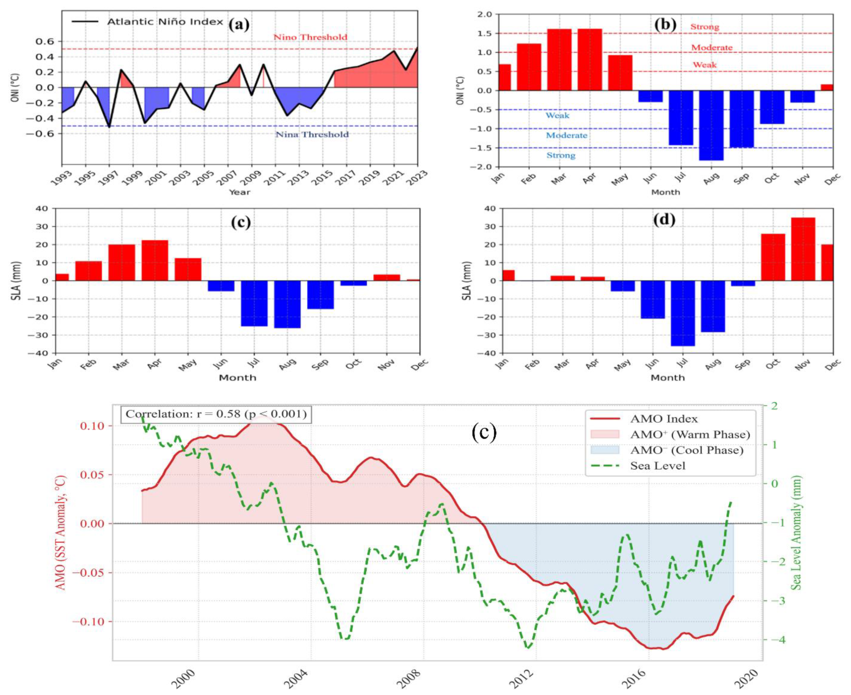
Sea level anomalies in the GoG are strongly modulated by large-scale climate modes, particularly ENSO and the AMO (Figure 13). The Oceanic Niño Index (ONI) reveals that major El Niño events (e.g., 2020–2023) coincide with elevated SLA in the northern GoG, peaking during boreal spring and autumn (Figure 13a). This response stems from a well-established teleconnection: positive SST anomalies in the equatorial Pacific weaken the Atlantic zonal SST gradient, displacing the ITCZ southward and enhancing rainfall and runoff over the GoG. The combined effect of freshwater input and wind-driven steric adjustments modulates SLA, producing seasonal maxima in April in the southern GoG and November in the northern GoG. These peaks primarily result from the lagged response to cumulative freshwater input, enhanced upper-ocean stratification, and fluvial discharge maxima.
Hydrological amplification is most pronounced in coastal zones with narrow shelves (e.g., Niger Delta, Bight of Benin), where saturated soils and dense river networks exacerbate runoff during El Niño. Conversely, La Niña phases suppress convection and SLA through cooler SSTs, strengthened easterlies, and reduced precipitation. This asymmetry underscores the nonlinearity of ENSO–SLA interactions, with El Niño generating larger, spatially coherent anomalies compared to La Niña’s weaker, diffuse signals (Figures 13b–d). Seasonal SLA patterns further reflect these dynamics, with March–May (southern GoG) and September–November (northern GoG) maxima aligning with ENSO-driven hydroclimatic forcing.
The AMO introduces a low-frequency modulation of SLA by altering North Atlantic SSTs, thereby affecting ITCZ position and WAM intensity (Figure 13f). Positive AMO phases, observed during 1993–2003 and 2018–2023, correspond with higher SLA in the GoG. These intervals align with strengthened WAM activity, increased moisture flux, and elevated runoff. In contrast, the intervening cool AMO phase (2005–2017) coincides with depressed SLA, weaker monsoon circulation, and reduced freshwater inflow. The SLA response to AMO operates through both steric and barotropic pathways, with long-term SST anomalies modulating wind stress, rainfall, and upper-ocean stratification across the tropical Atlantic. The co-occurrence of warm ENSO and AMO phases post-2015 contributed to record-high SLA anomalies in the GoG. This constructive interference illustrates the compounding effects of multiscale climate drivers, wherein interannual ENSO pulses are superimposed on the multidecadal AMO background. These compound forcing regimes contribute to SLA variability through synergistic effects on rainfall, runoff, wind stress, and stratification.
4. Discussion and Conclusion
The Gulf of Guinea has emerged as a hotspot of accelerated SLR, with satellite altimetry indicating a significant increase (p < 0.01) in the regional trend from 2.93 ± 0.1 mm yr⁻¹ (1993–2014) to 5.4 ± 0.25 mm yr⁻¹ (2015–2023). This shift reflects a transition from steric-dominated variability to a hybrid steric–manometric regime, where ocean mass redistribution now dominates the regional sea-level budget. GRACE/GRACE-FO data show an increase in mass contributions from 42 ± 4% to 58 ± 5% since 2015. Localized mass loading exceeds 10 mm yr⁻¹ near the Niger Delta and Cameroon coast, aligning with intensified precipitation over adjacent catchments. Post-2015 rainfall trends exceed 6 mm yr⁻¹, sustaining soil moisture saturation and enhancing terrestrial freshwater discharge. The GoG was recently identified as the global maximum in ocean mass increase driven by continental hydrology (McGirr et al., 2024).
The transition to mass-dominated sea-level rise has been facilitated by a reorganization of regional atmospheric circulation. ERA5 reanalysis shows a marked intensification of zonal winds (18 ± 4% increase in wind stress) and the development of a cyclonic wind stress curl anomaly in the eastern Gulf, which together have modified coastal dynamics through three primary mechanisms: (1) enhanced equatorial convergence suppressing offshore Ekman transport, (2) altered reflection characteristics of equatorial waves at the eastern boundary, and (3) increased downwelling-favorable winds along the northern coastline. These changes have substantially disrupted the basin’s waveguide dynamics. Whereas the pre-2015 regime was characterized by coherent propagation of eastward Kelvin waves transitioning to coastal trapped waves and reflected Rossby waves, the post-2015 period shows reduced thermocline tilting, decreased Rossby wave speeds, and diminished coherence between equatorial and coastal sea-level anomalies.
The wind stress anomalies are partly linked to large-scale modes, including a strengthening WAM and changes in equatorial easterlies, which further modulate nearshore wind stress curl and wave reflection characteristics. These adjustments in wind fields represent key couplings between tropical atmospheric variability and regional ocean dynamics. Rainfall–runoff timing has also enhanced terrestrial-ocean coupling. The seasonal overlap between peak river discharge and elevated nearshore wave energy or stratification reinforces coastal mass accumulation and density-driven circulation. This phase alignment strengthens the nonlinear interaction between surface forcing and boundary dynamics, amplifying sea-level variability near deltas and estuarine systems.
Interannual climate variability interacts with these local processes to generate nonlinear sea-level responses. Strong El Niño events elevate regional sea level through coupled steric and manometric mechanisms, atmospheric teleconnections enhance coastal precipitation (increasing mass input), while equatorial wind anomalies disrupt wave propagation. The 2022–2023 El Niño, coinciding with a warm AMO phase, produced the largest sea-level excursion of the altimetry era via this mechanism. On decadal scales, AMO modulates the background state—warm phases (1993–2003, 2018–present) intensify precipitation responses to ENSO events and strengthen WAM circulation, creating sustained mass-loading conditions.
Current climate models underestimate these regional sea-level responses, especially the terrestrial–marine coupling. CMIP6 ensemble members show a 20–45% underestimation of mass contributions (Slangen et al., 2017; Meyssignac et al., 2017), due to coarse coastal resolution and simplified land hydrology schemes. These biases compromise projections of regional sea-level change, particularly as anthropogenic warming intensifies the hydrological cycle and modifies tropical wave dynamics. Key uncertainties remain in isolating the relative roles of internal variability versus anthropogenic forcing in driving observed circulation shifts, and in assessing whether similar steric-to-mass transitions are occurring in other tropical marginal seas. Addressing these gaps requires enhanced observing systems to resolve interactions between terrestrial hydrology, coastal oceanography, and atmospheric dynamics, alongside regional climate models that explicitly couple land, ocean, and atmosphere. The Gulf of Guinea’s unique sea-level regime, shaped by both large-scale climate variability and regional hydrological processes, offers a critical testbed for improving understanding of coastal sea-level budgets under a changing climate.
References
- Adamec, D.; O’Brien, J.J. The seasonal upwelling in the Gulf of Guinea due to remote forcing. Journal of Physical Oceanography 1978, 8, 1050–1060. [Google Scholar] [CrossRef]
- Aman, A.; Testut, L.; Woodworth, P.L.; Aarup, A.; Dixon, D.J. Seasonal sea level variability in the Gulf of Guinea from altimetry and tide gauge. Revue Ivoirienne des Sciences et Technologie 2007, 9, 105–118. [Google Scholar]
- Ayinde, A.S.; Yu, H.; Wu, K. Sea level variability and modeling in the Gulf of Guinea using supervised machine learning. Scientific Reports 2023, 13, 21318. [Google Scholar] [CrossRef] [PubMed]
- Chelton, D.B.; DeSzoeke, R.A.; Schlax, M.G.; El Naggar, K.; Siwertz, N. Geographical variability of the first baroclinic Rossby radius of deformation. Journal of Physical Oceanography 1998, 28, 433–460. [Google Scholar] [CrossRef]
- Chen, X.; Zhang, X.; Church, J. A. , Watson, C. S., King, M. A., Monselesan, D., Legresy, B.; Harig, C. The increasing rate of global mean sea-level rise during 1993–2014. Nature Climate Change 2017, 7, 492–495. [Google Scholar] [CrossRef]
- Dangendorf, S.; Hay, C.; Calafat, F. M., et al. Persistent acceleration in global sea-level rise since the 1960s. Nature Climate Change 2019, 9, 705–710. [CrossRef]
- Dieng, H.B.; Dadou, I.; Léger, F.; Morel, Y.; Jouanno, J.; Lyard, F.; Allain, D. Sea level anomalies using altimetry, model and tide gauges along the African coasts in the Eastern Tropical Atlantic Ocean: Inter-comparison and temporal variability. Advances in Space Research 2021, 68, 534–552. [Google Scholar] [CrossRef]
- Evadzi, P.I.K.; Zorita, E.; Hünicke, B. West African sea level variability under a changing climate: What can we learn from the observational period? Journal of Coastal Conservation 2019, 23, 759–771. [Google Scholar] [CrossRef]
- Fox-Kemper, B.; Hewitt, H.T.; Xiao, C.; Aðalgeirsdóttir, G.; Drijfhout, S.S.; Edwards, T.L.; Golledge, N.R.; Hemer, M.; Kopp, R.E.; Krinner, G. and Mix, A., 2021. Ocean, cryosphere and sea level change. Climate change 2021: the physical science basis. Contribution of Working Group I to the Sixth Assessment Report of the Intergovernmental Panel on Climate Change. Climate Change. Ghomsi, K. F. E., Raj, R. P., Bonaduce, A., Halo, I., Nyberg, B., Cazenave, A., ... & Johannessen, O. M. (2024). Sea level variability in the Gulf of Guinea from satellite altimetry. Scientific Reports, 14(1), 4759.
- Fox-Kemper, B.; Hewitt, H.T.; Xiao, C.; Aðalgeirsdóttir, G.; Drijfhout, S.S.; Edwards, T.L.; Golledge, N.R.; Hemer, M.; Kopp, R.E.; Krinner, G.; Mix, A. Ocean, cryosphere and sea level change. Climate change 2021: the physical science basis. Contribution of Working Group I to the Sixth Assessment Report of the Intergovernmental Panel on Climate Change. Climate Change, 2021. [Google Scholar]
- Good, S.A.; Martin, M.J. and Rayner, N.A. EN4: Quality controlled ocean temperature and salinity profiles and monthly objective analyses with uncertainty estimates. Journal of Geophysical Research: Oceans 2013, 118, 6704–6716. [Google Scholar] [CrossRef]
- Iler, A.M.; Inouye, D.W.; Schmidt, N.M.; Høye, T.T. Detrending phenological time series improves climate–phenology analyses and reveals evidence of plasticity. 2017. [Google Scholar]
- IPCC (2023). Lee, H., Calvin, K., Dasgupta, D., Krinner, G., Mukherji, A., Thorne, P., Trisos, C., Romero, J., Aldunce, P., Barret, K., and Blanco, G., 2023. Climate Change 2023: Synthesis Report, Summary for Policymakers. Contribution of Working Groups I, II, and III to the Sixth Assessment Report of the Intergovernmental Panel on Climate Change [Core Writing Team, H. Lee and J. Romero (eds.)]. IPCC, Geneva, Switzerland.
- Longhurst, A.R. A review of the oceanography of the Gulf of Guinea. Bulletin de l’Institut Français d’Afrique Noire Série A Sciences Naturelles 1962, 24, 633–663. [Google Scholar]
- Lorenz, E.N., 1956. Empirical orthogonal functions and statistical weather prediction. (No Title).
- Kendall, M. G., 1975. Rank correlation methods. Griffin, London.
- Kemgang Ghomsi, F.E.; Raj, R.P.; Bonaduce, A.; Halo, I.; Nyberg, B.; Cazenave, A.; Rouault, M.; Johannessen, O.M. Sea level variability in Gulf of Guinea from satellite altimetry . Scientific Reports 2024, 14, 4759. [Google Scholar] [CrossRef]
- Mann, H. B. Nonparametric tests against trend. Econometrica 1945, 245–259. [Google Scholar] [CrossRef]
- McGirr, R.; Tregoning, P.; Purcell, A.; McQueen, H. Significant local sea level variations caused by continental hydrology signals. Geophysical Research Letters 2024, 51, e2024GL108394. [Google Scholar] [CrossRef]
- Meyssignac, B.; Slangen, A.A.; Melet, A.; Church, J.A.; Fettweis, X.; Marzeion, B.; Agosta, C.; Ligtenberg, S.R.M.; Spada, G.; Richter, K. and Palmer, M.D. Evaluating model simulations of twentieth-century sea-level rise. Part II: Regional sea-level changes. Journal of Climate 2017, 30, 8565–8593. [Google Scholar] [CrossRef]
- North, G.R.; Bell, T.L.; Cahalan, R.F.; Moeng, F.J. Sampling errors in the estimation of empirical orthogonal functions. Monthly weather review 1982, 110, 699–706. [Google Scholar] [CrossRef]
- Oppenheimer, M.; Glavovic, B.; Hinkel, J.; Van de Wal, R.; Magnan, A.K.; Abd-Elgawad, A.; Cai, R.; Cifuentes-Jara, M.; Deconto, R.M.; Ghosh, T.; Hay, J. Sea level rise and implications for low lying islands, coasts and communities.
- Peltier, W.R.; Argus, D.F.; Drummond, R. Space geodesy constrains ice age terminal deglaciation: The global ICE-6G_C (VM5a) model. Journal of Geophysical Research: Solid Earth 2015, 120, 450–487. [Google Scholar] [CrossRef]
- Rodríguez-Fonseca, B.; Polo, I.; García-Serrano, J.; Losada, T.; Mohino, E.; Mechoso, C.R. and Kucharski, F., 2009. Are Atlantic Niños enhancing Pacific ENSO events in recent decades? . Geophysical Research Letters 2009, 36. [Google Scholar]
- Sen, P.K. Estimates of the regression coefficient based on Kendall’s tau. Journal of the American Statistical Association 1968, 63, 1379–1389. [Google Scholar] [CrossRef]
- Slangen, A.B.; Meyssignac, B.; Agosta, C.; Champollion, N.; Church, J.A.; Fettweis, X.; Ligtenberg, S.R.; Marzeion, B.; Melet, A.; Palmer, M.D. and Richter, K. Evaluating model simulations of twentieth-century sea level rise. Part I: Global mean sea level change. Journal of Climate 2017, 30, 8539–8563. [Google Scholar] [CrossRef]
- Spall, M.A.; Pedlosky, J. Reflection and transmission of equatorial Rossby waves. Journal of physical oceanography 2005, 35, 363–373. [Google Scholar] [CrossRef]
- Swenson, S.; Chambers, D.; Wahr, J. Estimating geocenter variations from a combination of GRACE and ocean model output. Journal of Geophysical Research: Solid Earth 2008, 113. [Google Scholar] [CrossRef]
- Theil, H. A rank-invariant method of linear and polynomial regression analysis. In Proceedings of the Netherlands Academy of Arts and Sciences (Vol. 1950). Springer.
- Thorncroft, C.D.; Nguyen, H.; Zhang, C.; Peyrillé, P. Annual cycle of the West African monsoon: regional circulations and associated water vapour transport. Quarterly Journal of the Royal Meteorological Society 2011, 137, 129–147. [Google Scholar] [CrossRef]
- Vellinga, M.; Arribas, A. and Graham, R., 2013. Seasonal forecasts for regional onset of the West African monsoon. Climate Dynamics 2013, 40, 3047–3070. [Google Scholar] [CrossRef]
- Verstraete, J.M. The seasonal upwellings in the Gulf of Guinea. Progress in Oceanography 1992, 29, 1–60. [Google Scholar] [CrossRef]
- Von Storch, H. and Zwiers, F.W. Statistical analysis in climate research. Cambridge university press.
- Wahr, J.; Molenaar, M.; Bryan, F. Time variability of the Earth’s gravity field: Hydrological and oceanic effects and their possible detection using GRACE. Journal of Geophysical Research: Solid Earth 1998, 103, 30205–30229. [Google Scholar] [CrossRef]
- Xie, S.P.; Carton, J.A. Tropical Atlantic variability: Patterns, mechanisms, and impacts. Earth’s Climate: The Ocean–Atmosphere Interaction, Geophys. Monogr 2004, 147, pp. [Google Scholar]
Figure 1.
Bathymetric map of the Gulf of Guinea based on the GEBCO 15-arc-second global dataset (https://www.gebco.net), showing seafloor depths >10 m. Major surface currents influencing regional ocean dynamics are overlaid. National boundaries and labels provide geographic context.
Figure 1.
Bathymetric map of the Gulf of Guinea based on the GEBCO 15-arc-second global dataset (https://www.gebco.net), showing seafloor depths >10 m. Major surface currents influencing regional ocean dynamics are overlaid. National boundaries and labels provide geographic context.
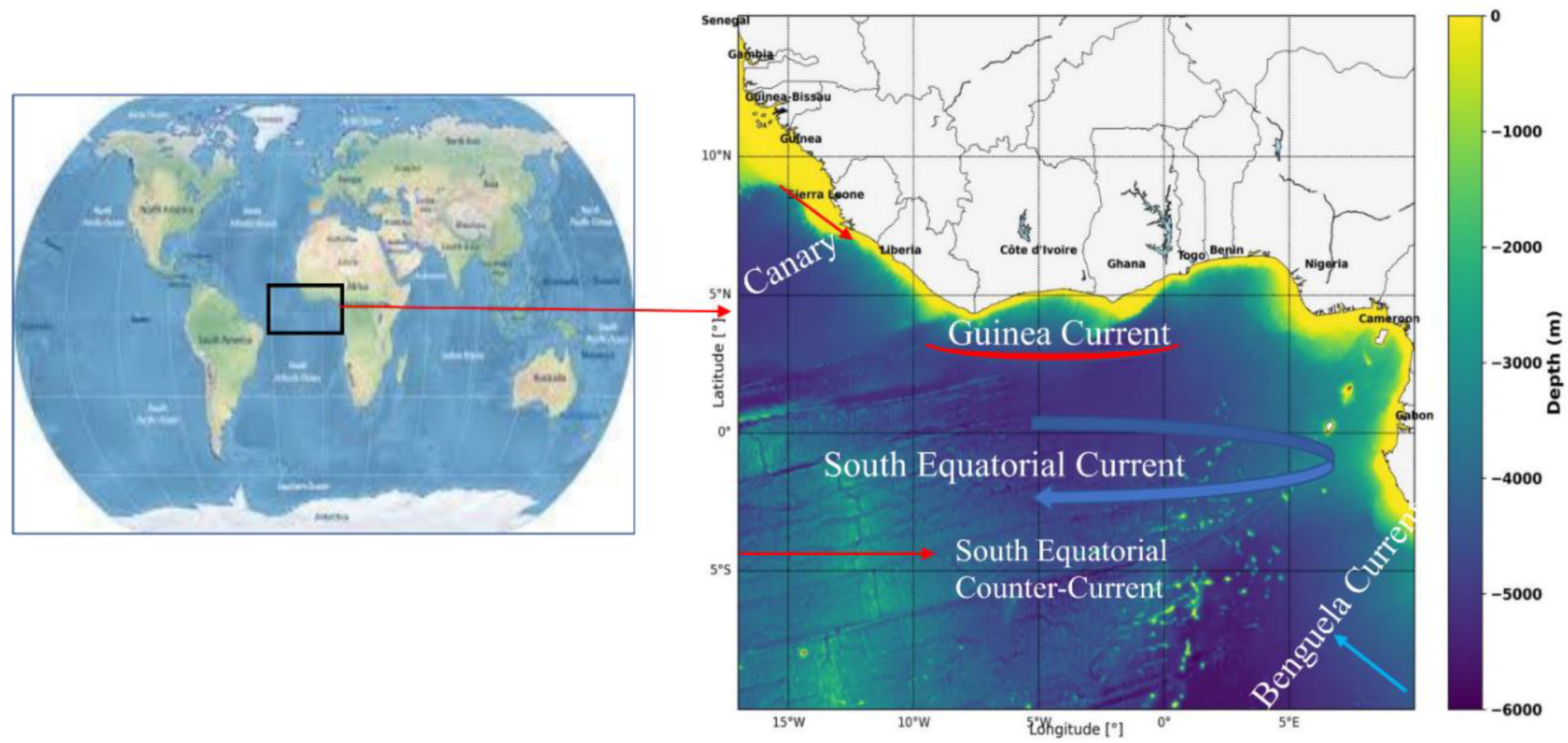
Figure 2.
The temporal heterogeneity in the rate of sea level rise, derived from gridded CMEMS satellite altimetry data, showing a notable shift in the rate of increase from 1993–2014 to 2015–2023 (a); the long-term temporal evolution of regional sea level rise (red) is presented alongside its dominant contributing components: ocean mass redistribution (OMR) derived from GRACE-FO data (2002–2023) (blue) and sterodynamic sea level change (1993–2023) (green) (b). All components are smoothed using a 3-year moving average filter.
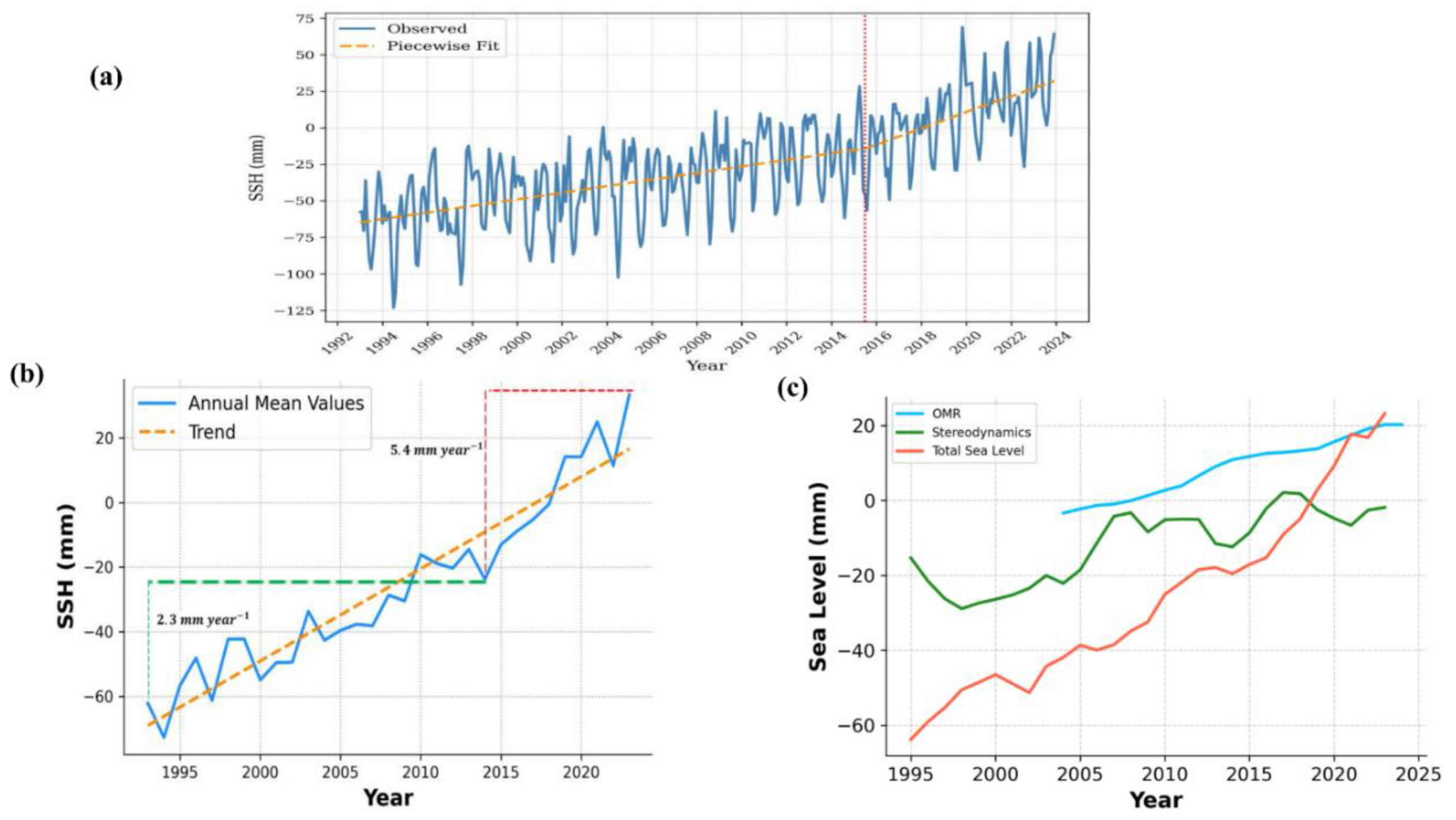
Figure 3.
The observed the observed SLA (blue line) with the fitted trend using B-spline smoothing (red line) from the Generalized Additive Mixed Model (GAMM) (a); the residual distribution from the model, represented as a histogram (sky blue) with an overlaid kernel density estimate (KDE) curve, highlighting the residual pattern (b).
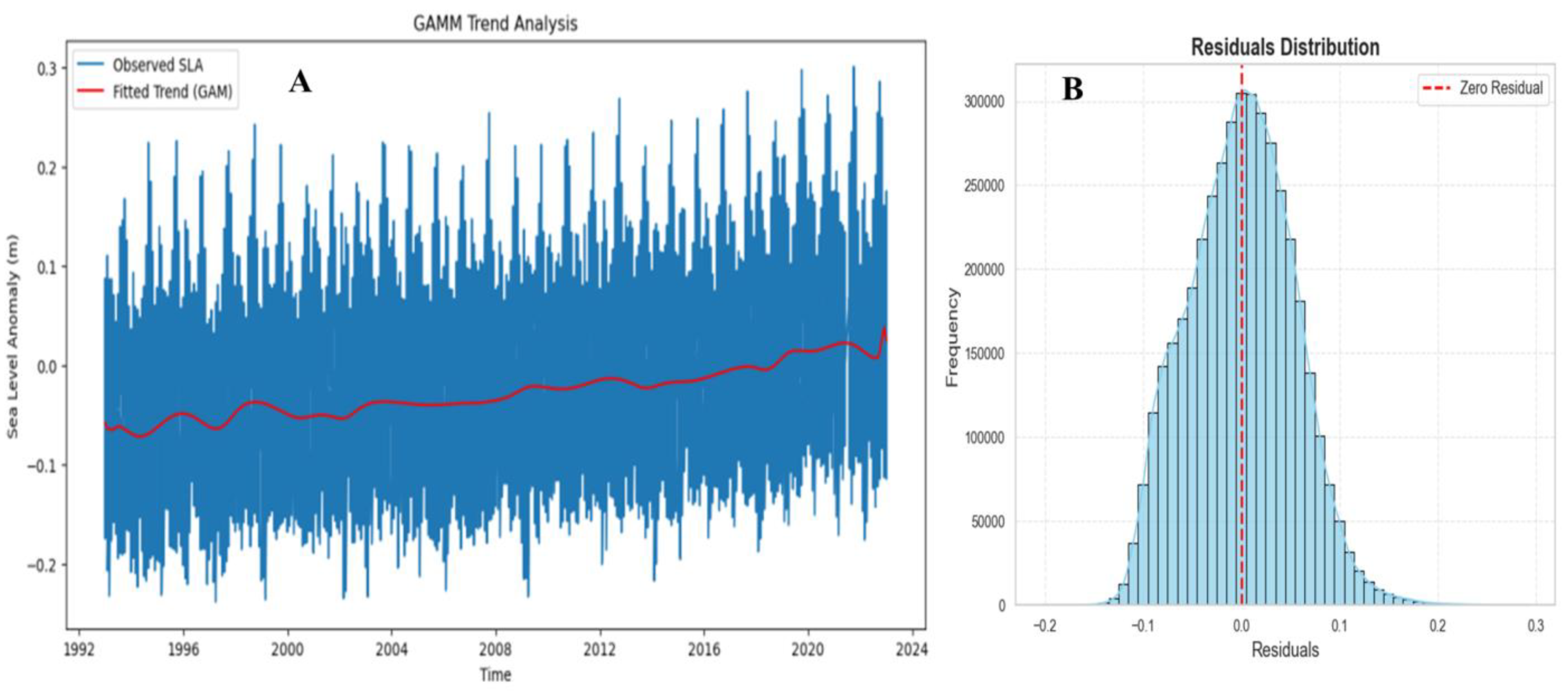
Figure 4.
The autocorrelation function (ACF) of mean SLA values over 40 monthly lags highlights significant peaks at 12, 24, and 36 months (red-blue arrows). The black dashed line represents zero autocorrelation, while the red dashed lines denote the 95% confidence interval. The gradual decay of autocorrelation values indicates the persistence of temporal correlations (a). The Power Spectral Density (PSD) of SLA shows variance distribution across log-scaled periods (x-axis, in years) and PSD values (y-axis). Log-period scaling, following oceanographic convention, enhances resolution of seasonal to decadal variability and highlights dominant climate modes (b).
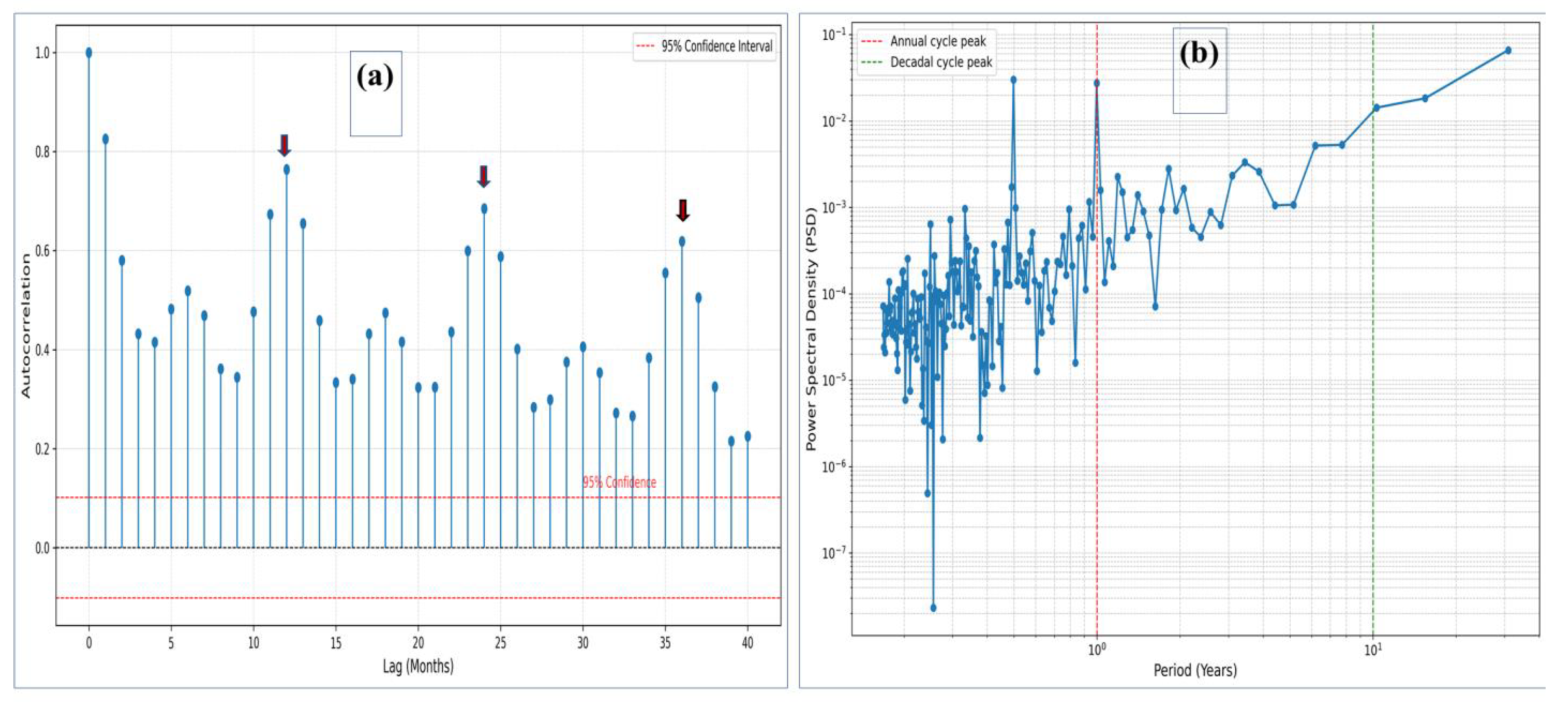
Figure 5.
Linear sea level trends derived from the ordinary least squares (OLS) method, illustrating spatial variability across the Gulf of Guinea. (a) OMR trend (2002–2023), highlighting its strong influence in the southern basin. (b) Sterodynamic sea level change (1993–2023), showing its dominance in the northern Gulf. (c) Sea level anomaly (SLA) trend (1993–2023) reveals variability and rapid acceleration along the northern basin. (d–f) Recent linear trends for 2015–2023: (d) OMR, (e) sterodynamic sea level, and (f) SLA, which exceeds the global mean sea level (GSML).
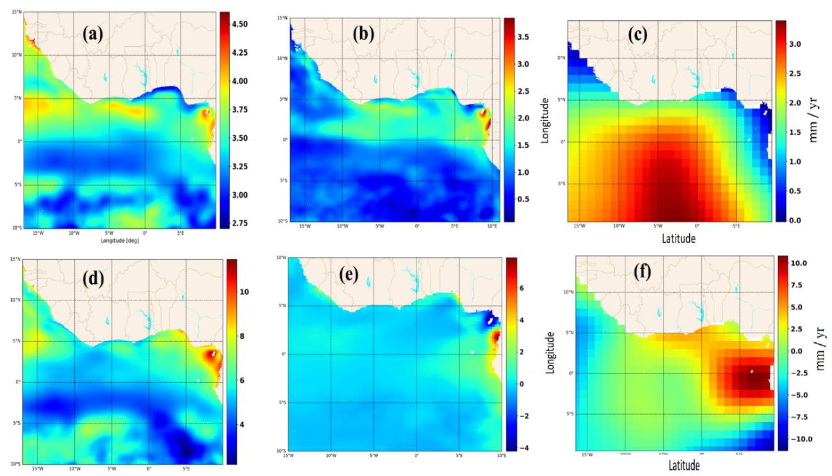
Figure 6.
The first three leading Empirical Orthogonal Function (EOF) modes of interannual SLA variability in the Gulf of Guinea (GoG) highlight dynamic sea level changes over two distinct periods. (a) EOF modes for 1993–2014, explaining 57%, 19%, and 11% of the total variance, respectively. (b) EOF modes for 2015–2023, capturing 59%, 16%, and 12% of the variance, respectively. (c) The trend and correlation between the principal component of the third EOF mode (PC3) and the Atlantic Meridional Overturning Circulation (AMOC) index (1993-2021). (d) The corresponding bottom bar plots include 95% confidence intervals derived from 1,000 bootstrap resamples, quantifying uncertainty in the variance estimates.
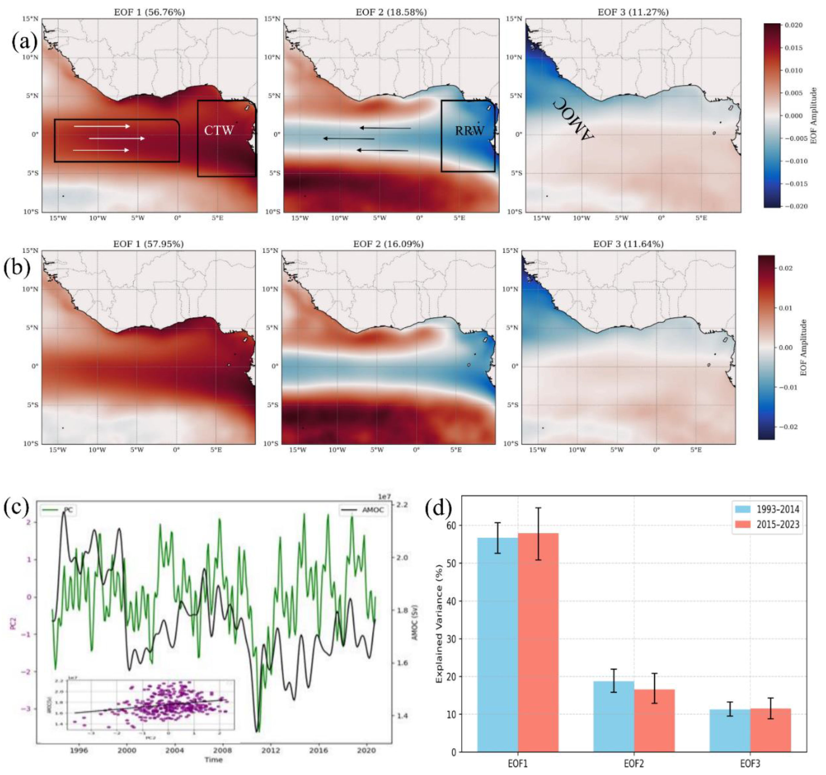
Figure 7.
(a) Two-dimensional power spectral density of SLA along the equatorial band (5°S–5°N), derived from Fast Fourier Transform (FFT) analysis. The left panel shows log-scaled spectral power as a function of frequency (cycles/day) and zonal wavenumber (cycles/degree); the right panel isolates westward-propagating signals (negative wavenumbers, k < 0). The red marker highlights the dominant mode with a 59.9-day period and ~30° wavelength, consistent with first-mode equatorial Rossby wave dynamics. (b) Hovmöller diagram of equatorial SLA showing eastward-propagating features. Horizontal dashed lines indicate the theoretical phase speed (2.8 m/s) of first-mode baroclinic Kelvin waves. (c) Hovmöller diagram emphasizing westward-propagating SLA signals. Diagonal trajectories align with the spectral mode identified in (a), supporting the presence of Rossby wave activity across the equatorial Atlantic.
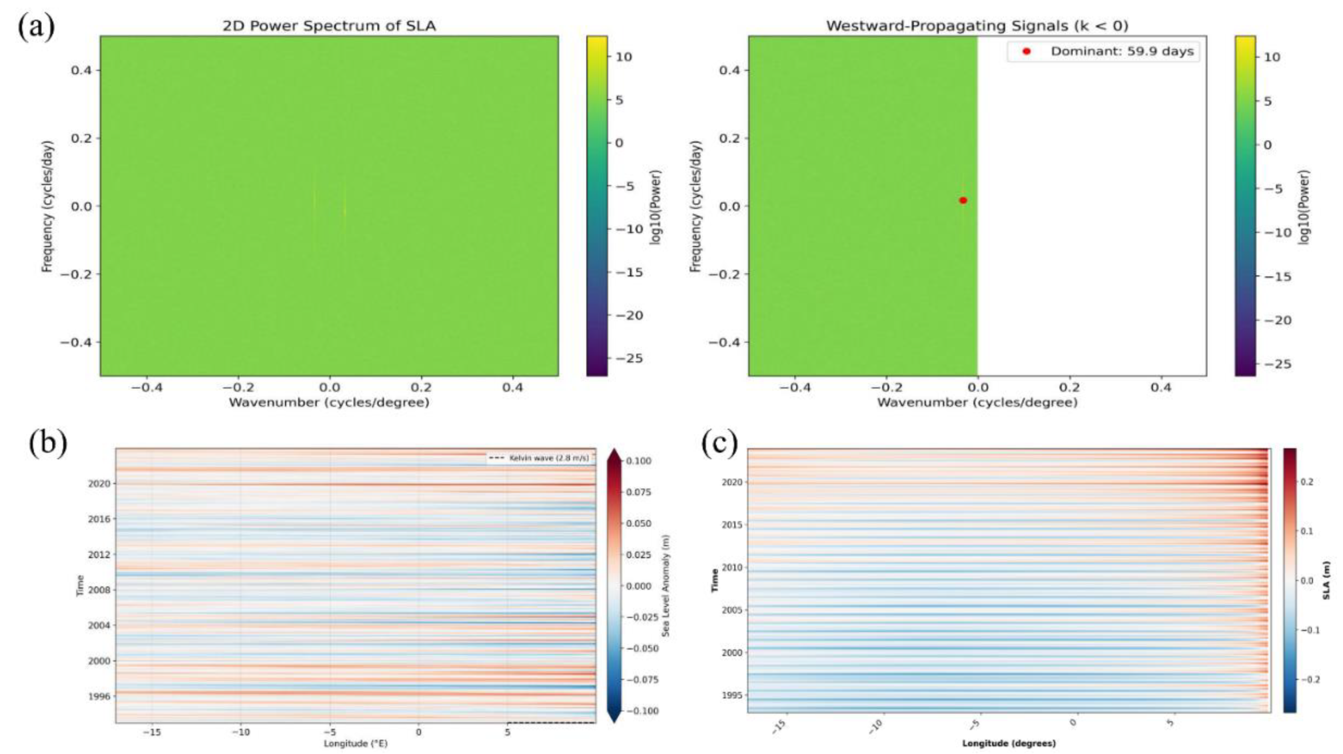
Figure 8.
The comparison between the observed SLA (solid blue line) and the predicted SLA (dashed orange line) is derived using a Random Forest Regression (RFR) model with forcing variables as predictors. It also presents the feature importance of the RFR model, displayed as a horizontal bar chart, illustrating the magnitude of the contribution of each predictor to the model. Adapted from Ayinde et al., 2023.
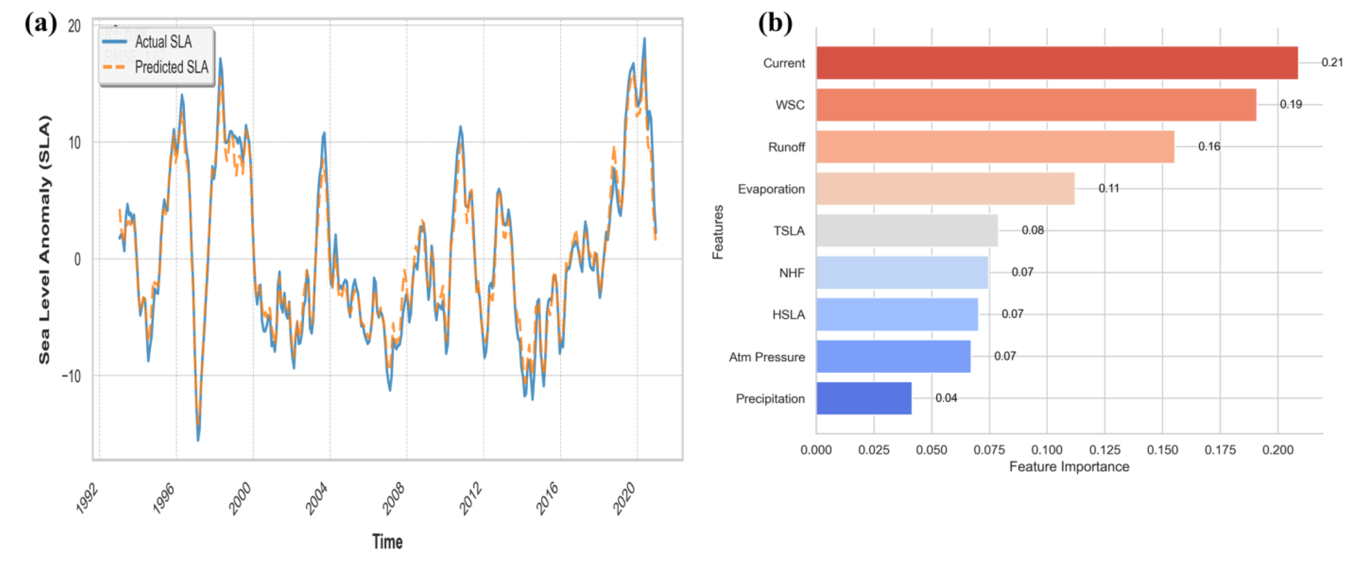
Figure 9.
First empirical orthogonal function (EOF1) modes of zonal wind stress and precipitation over the Gulf of Guinea, shown separately for two periods: (a1–a2) Zonal wind EOF1 spatial patterns for 1993–2014 and 2015–2023; (b1–b2) Precipitation EOF1 spatial patterns for 1993–2014 and 2015–2023. (c) Normalized time series of PC1 for wind and precipitation, alongside total runoff, compared with regional SLA anomalies over 1993–2023. (d) Cross-correlation functions between SLA and wind PC1 (blue), and SLA and precipitation PC1 (green), showing leading-lagging relationships.
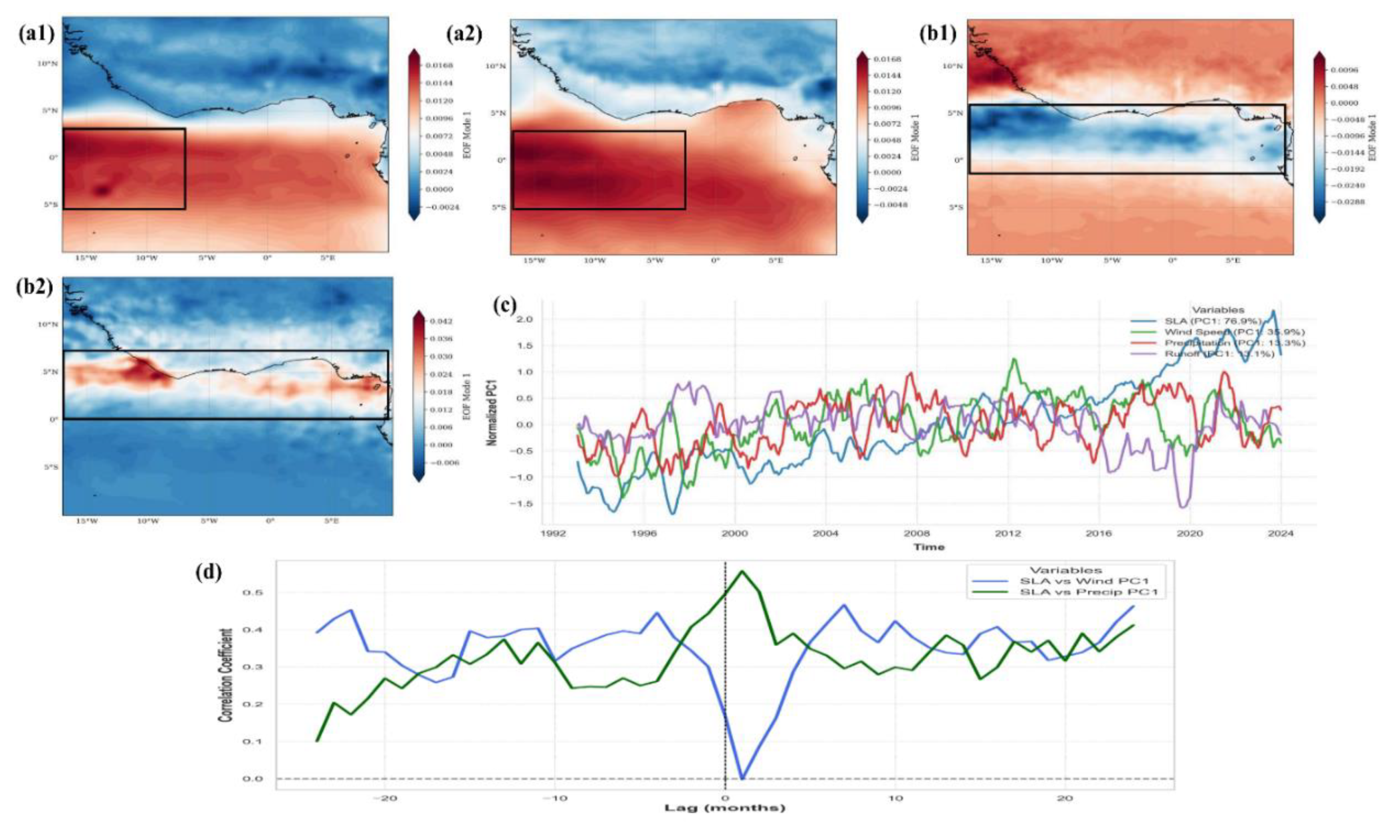
Figure 10.
Linear trends in surface wind and precipitation over the Gulf of Guinea during two periods: (a1–a2) Wind vector magnitude and direction trends for 1993–2014 and 2015–2023;(b1–b2) Precipitation trends for 1993–2014 and 2015–2023. Red boxes indicate regions of statistically significant change, highlighting zones of recent intensification in atmospheric dynamics. (c) Cross-correlation functions between SLA and wind PC1 (blue), and SLA and precipitation PC1 (green), showing lagged responses and temporal coupling with sea-level variability.
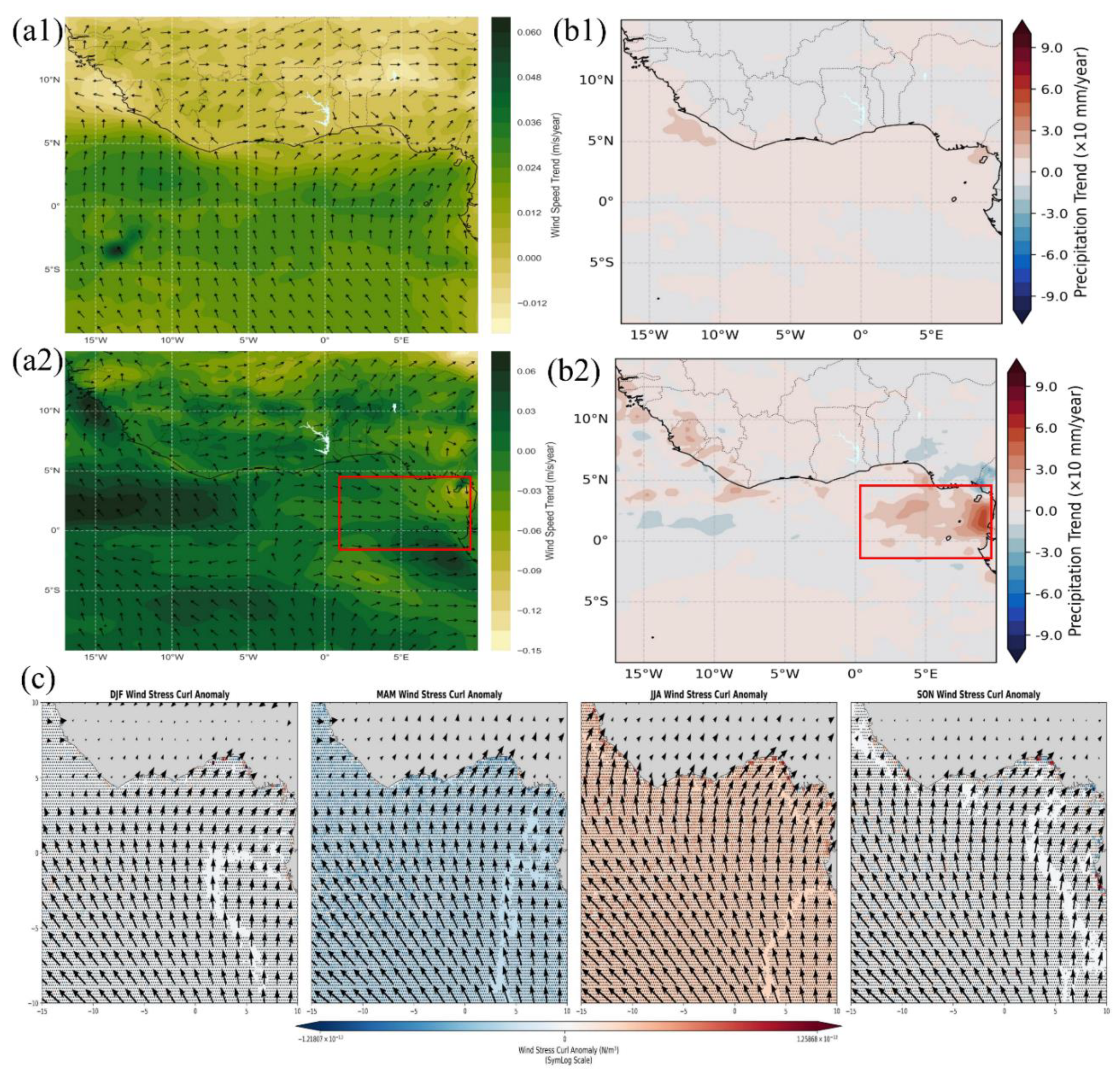
Figure 11.
Spatial trends in seasonal variability of (a) sea level anomaly (SLA) and (b) precipitation across the Gulf of Guinea from 1993 to 2023, derived from monthly mean values at each grid point. The panels reveal strong seasonal heterogeneity between the northern and southern sub-basins. Red boxes indicate zones of pronounced SLA and rainfall divergence, reflecting spatially distinct ocean–atmosphere interactions across the basin.
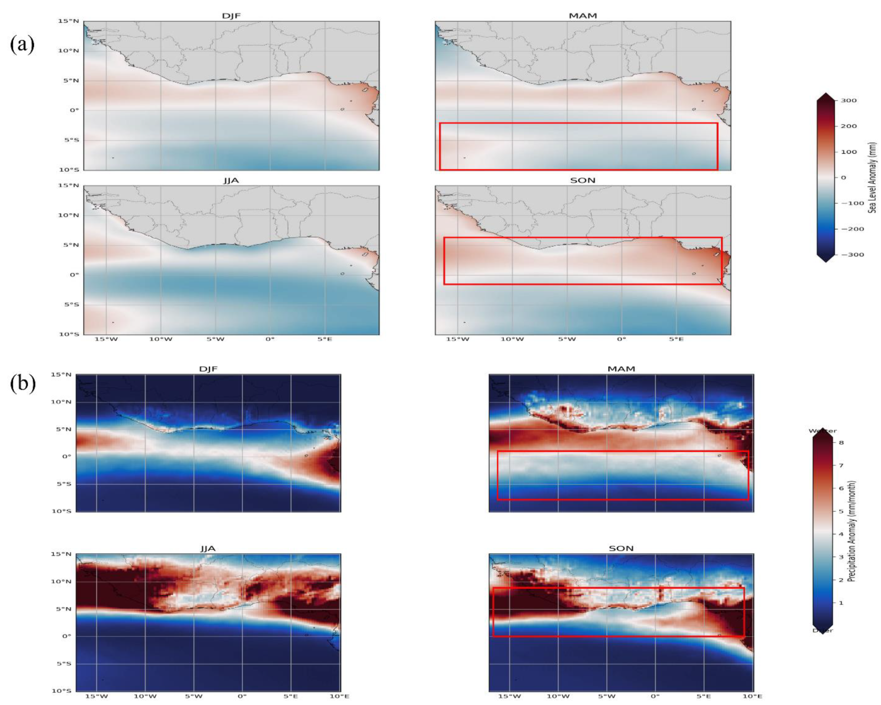
Figure 12.
Spatial Pearson correlation between SLA and sterodynamic components for (a1) 1993–2014 and (a2) 2015–2023, and between SLA and OMR for (b1) 1993–2014 and (b2) 2015–2023.
Figure 12.
Spatial Pearson correlation between SLA and sterodynamic components for (a1) 1993–2014 and (a2) 2015–2023, and between SLA and OMR for (b1) 1993–2014 and (b2) 2015–2023.
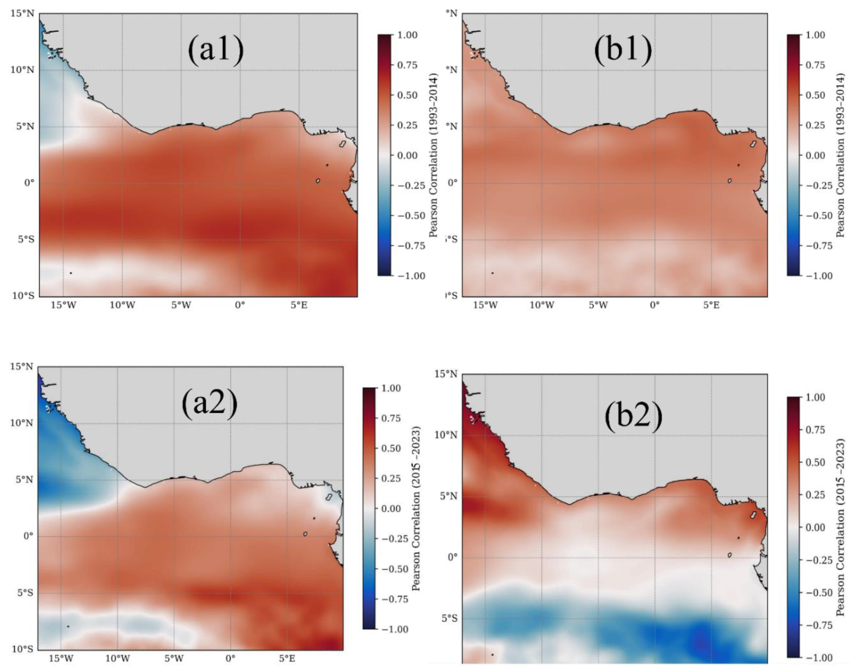
Figure 13.
Time series of the Atlantic Niño Index (ONI) from 1993 to 2023, representing the sea surface temperature anomaly in the Atlantic Ocean region (5°S to 5°N, 30°W to 10°W), positive values indicate Niño conditions (red shading), while negative values correspond to Niña conditions (blue shading). The dashed red and blue lines represent threshold values for Niño and Niña events, respectively (a); Monthly time series of the ONI. Positive values (shown in red) represent Niño conditions, while negative values (shown in blue) correspond to Niña conditions. The red dashed lines at 0.5, 1.0, and 1.5 denote weak, moderate, and strong Niño thresholds, respectively, while the blue dashed lines at -0.5, -1.0, and -1.5 indicate weak, moderate, and strong Niña conditions (b); Monthly time series of the SLA along the northern basin with positive anomalies (shown in red) indicate regions of higher-than-average sea level, while negative anomalies (shown in blue) represent lower-than-average sea level (c); and along the southern basin (d).
Disclaimer/Publisher’s Note: The statements, opinions and data contained in all publications are solely those of the individual author(s) and contributor(s) and not of MDPI and/or the editor(s). MDPI and/or the editor(s) disclaim responsibility for any injury to people or property resulting from any ideas, methods, instructions or products referred to in the content. |
© 2025 by the authors. Licensee MDPI, Basel, Switzerland. This article is an open access article distributed under the terms and conditions of the Creative Commons Attribution (CC BY) license (http://creativecommons.org/licenses/by/4.0/).
Copyright: This open access article is published under a Creative Commons CC BY 4.0 license, which permit the free download, distribution, and reuse, provided that the author and preprint are cited in any reuse.


