

Submitted:
29 July 2025
Posted:
30 July 2025
Read the latest preprint version here
Abstract
This study develops an integrated risk modeling framework to assess capital adequacy and optimize portfolio performance for Thai life and non-life insurers. Combining ARMA–GJR–GARCH models with skewed Student-t innovations, Extreme Value Theory, and dynamic R-vine copulas captures volatility, tail risks, and evolving asset interdependencies. Using daily data from 2014 to 2024, the models generate Value-at-Risk forecasts and rolling Sharpe ratios for portfolios with and without green bonds. Results show that green bond inclusion improves risk-adjusted returns and reduces capital requirements, particularly for life insurers, aligning with their long-term solvency mandates. Although a greenium effect is not clearly observed relative to Thai sovereign bonds, green bonds enhance diversification within a multivariate framework. These findings highlight the importance of evaluating capital requirements at the portfolio level and suggest that regulators incorporate ESG considerations into supervisory investment guidelines to strengthen financial resilience and align the insurance sector with Thailand’s sustainable finance goals.
Keywords:
green bonds
; dynamic r-vine copulas
; extreme value theory
; insurance capital adequacy
; value-at-risk
1. Introduction
Robust risk modeling is crucial for modern insurance portfolio management, especially for life and non-life insurers navigating volatile markets. Traditional approaches often fail to capture tail risks and nonlinear dynamics, particularly during stress periods. As regulatory demands tighten under solvency frameworks, insurers increasingly require advanced modeling techniques to accurately assess volatility and extreme losses (Bollerslev, 1986; Daly, 2008).
Insurance companies are increasingly integrating Environmental, Social, and Governance (ESG) considerations into their investment strategies to strengthen portfolio resilience and support long-term sustainability goals. Among ESG instruments, green bonds have emerged as a compelling asset class, channeling funds into projects such as renewable energy and low-carbon infrastructure (Climate Bonds Initiative, 2022). Their dual potential to generate financial returns and promote sustainability has attracted insurers seeking diversification and alignment with ESG mandates (Ferrer et al., 2021; Han et al., 2024; Karim et al., 2024; Park et al., 2020; Papavassiliou et al., 2025). Green bonds have also been associated with improved Sharpe ratios and reduced capital charges under solvency frameworks (Taghizadeh-Hesary et al., 2021; Zhang et al., 2021). In Thailand, where insurers manage sizable and duration-sensitive portfolios, green bond inclusion supports both financial stability and national sustainability objectives (Fitrah and Soemitra, 2022; Ramadhan, 2020). Regulatory support is central to enabling this transition. Tools such as green taxonomies, favorable capital treatment, and targeted incentives can accelerate ESG adoption across the sector (Flammer, 2020; Huang and Lin, 2023; Okeke et al., 2024). Recognizing the strong risk-adjusted performance of green bonds, the Office of Insurance Commission (OIC) could facilitate their broader adoption by incorporating sustainability-related investment guidance into supervisory frameworks. This would help insurers align investment strategies with solvency goals while advancing Thailand’s sustainable finance agenda.
Advanced financial econometrics provides crucial tools for modeling the complex risks faced by insurers. The Autoregressive Moving Average Generalized Autoregressive Conditional Heteroskedasticity (ARMA–GARCH) model, especially with the Glosten–Jagannathan–Runkle (GJR) extension, is valuable for capturing volatility clustering and asymmetric shock responses (Adegboyo and Sarwar, 2025; Glosten et al., 1993; Hidayana et al., 2021; Ma et al., 2024; Wei et al., 2025). The GJR–GARCH model accounts for the leverage effect, where negative shocks induce greater volatility than positive ones (Liu and Hung, 2010). Financial returns often exhibit skewness and fat tails, which, if unaccounted for, can lead to underestimation of risk. To address this, skewed Student-t innovations are widely adopted to improve Value-at-Risk (VaR) accuracy and better capture these distributional properties (Akanbi et al., 2025; Al-Khasawneh et al., 2024; Hansen, 1994; Harvey and Siddique, 1999; Lambert and Laurent, 2001; Patra and Gupta, 2025). However, even these enhanced models may underestimate extreme losses. Extreme Value Theory (EVT), particularly through the Generalized Pareto Distribution (GPD), enhances tail risk modeling by focusing on exceedances beyond a high threshold (Braione and Scholtes, 2016; Majumder, 2018). When applied to GARCH-filtered residuals, EVT improves VaR estimation under stress conditions, which is crucial for insurers operating under solvency requirements (Chen et al., 2024; Okou and Amar, 2023).
Insurers require methods that capture interdependence among assets, moving beyond univariate modeling. Correlation matrices often fail to reflect nonlinear and time-varying relationships, particularly during periods of financial distress. Copula models address this limitation by constructing flexible joint distributions. R-vine copulas are well suited for modeling complex dependency structures using sequences of bivariate copulas (Brechmann and Czado, 2013). Their dynamic extensions allow dependencies to evolve over time, which is essential for capturing contagion effects and shifts in market conditions (Raza et al., 2025; Zhou and Ji, 2021). When integrated with GARCH-based marginal models, this approach offers significant advantages for multivariate risk modeling. It enhances portfolio-level risk assessment and supports the design of capital-efficient, ESG-aligned investment strategies.
This study integrates ARMA–GJR–GARCH models with skewed Student-t innovations, EVT, and dynamic R-vine copulas into a unified framework tailored for insurer portfolios. Capturing volatility dynamics, tail risks, and evolving interdependencies, the framework improves VaR estimation and Sharpe ratio assessment under both normal and stressed conditions (Ahmadi et al., 2023; Han and Li, 2022; Jeleskovic et al., 2024). Using daily data on Thai financial assets and green bonds from 2014 to 2024, the study evaluates VaR forecasts and rolling Sharpe ratios across optimized portfolios. Results reveal that green bond inclusion enhances insurer portfolio performance, strengthens capital adequacy, improves risk-adjusted returns through diversification, and supports alignment with Thailand’s sustainability goals. This research offers practical insights for risk practitioners and regulators in emerging markets. The proposed framework enables more accurate capital requirement calculations and supports ESG integration within supervisory investment guidelines, crucial as Thai regulatory guidance, market maturity, and sustainability commitments rapidly evolve.
The remainder of this paper is structured as follows: Section 2 describes the dataset and methodology, including model specifications and validation procedures. Section 3 presents empirical findings and discussions on VaR forecasting, backtesting, and portfolio performance analysis. Section 4 concludes with key findings, policy implications, and suggestions for future research directions.
2. Domain of Experiment and Methodology
This study analyzes a comprehensive dataset of 2,869 daily observations spanning January 1, 2014, to December 31, 2024, using logarithmic returns. Logarithmic returns were calculated using the formula , where is the price at time t and is the price at time t 1. The dataset encompasses a variety of significant Thai financial assets: the SET Index, the Dubai crude oil, the Thai bullion gold, the 3-7-year government bond Index, the 7-10-year government bond Index, the JPY/THB exchange rate, the Property sector Index, and the Bloomberg Barclays MSCI US Green Bond Index. Data, obtained from Datastream International and Bloomberg, exhibit statistical properties typical of financial time series. With the exception of the exchange rate, the series display negative skewness, indicating a higher likelihood of large negative returns. High kurtosis values confirm leptokurtosis in most series, indicating a greater concentration around the mean and fatter tails than expected under normality, suggestive of increased extreme events. The Jarque–Bera (JB) test indicates that gold returns are normally distributed, unlike the other assets. The Augmented Dickey-Fuller (ADF) test results confirm that all series are stationary. Table 1 presents the summary statistics of daily returns for all eight assets examined in this study.
2.1. Autoregressive Moving Average Glosten–Jagannathan–Runkle Generalized Autoregressive Conditional Heteroskedasticity with Skewed Student-t Innovations
This study addresses key complexities in financial time series, such as volatility clustering, fat tails, and asymmetric shock responses, across eight asset classes, including green bonds. To model individual asset dynamics, it adopts the Autoregressive Moving Average–Glosten–Jagannathan–Runkle Generalized Autoregressive Conditional Heteroskedasticity (ARMA–GJR–GARCH) model with skewed Student-t innovations, jointly modeling the conditional mean and variance of returns. Portfolios of five and six assets (including green bonds) are then constructed by maximizing the Sharpe Ratio using Dynamic R-vine Copulas. This integrated approach offers a flexible and robust structure for volatility modeling and risk forecasting. To capture excess kurtosis and skewness common in financial return distributions, the innovation term follows the skewed Student-t distribution introduced by Hansen (1994). This distribution accounts for both fat tails and asymmetry, enhancing the precision of Value-at-Risk (VaR) estimates under both normal and extreme market conditions.
The GJR component is central to capturing asymmetric volatility in response to shocks, an effect often observed in financial markets. In the general ARMA(m,n)–GJR–GARCH(p,q) model, p represents the number of ARCH terms (lagged squared residuals) and asymmetry terms, while q denotes the number of GARCH terms (lagged conditional variances). Estimating mean and variance with skewed Student-t innovations, the model is given by:
In this model, represents the return of the time series at time t, and is the constant mean. The autoregressive coefficients capture the influence of past returns (AR part of order m), while the moving average coefficients account for the impact of past shocks (MA part of order n). The innovation term represents unpredictable shocks, modeled as the product of the conditional standard deviation and a shock , which follows a skewed Student-t distribution with zero mean and unit variance.
The skewed Student-t distribution is parameterized by degrees of freedom > 2 to ensure finite variance and a skewness parameter , where corresponds to the symmetric Student-t distribution. Its density function is defined as:
where constants , and are given by:
The conditional variance equation under the GJR–GARCH(p,q) specification is:
The constant helps ensure the variance remains positive. The ARCH terms represent the effects of lagged squared shocks, while the GARCH terms capture the persistence of volatility through lagged conditional variances. The asymmetry terms , together with the indicator function , allow the model to distinguish between the effects of positive and negative shocks. This indicator equals 1 when the lagged shock is negative, and 0 otherwise.
Under this specification, a positive shock contributes to the conditional variance, whereas a negative shock contributes . A positive and statistically significant indicates a leverage effect, meaning that negative shocks have a greater impact on volatility than positive shocks of the same magnitude. The GJR–GARCH model is particularly relevant for analyzing assets like green bonds, which may react asymmetrically to environmental developments or policy shifts. While the ARMA component captures serial dependence in returns, GJR–GARCH effectively models both volatility persistence and its asymmetric responses.
Model selection involved a systematic search over ARMA–GJR–GARCH specifications by varying the parameters m, n, p, and q. Each model was estimated using pseudo-maximum likelihood and validated through residual diagnostics to ensure zero mean, homoscedasticity, and no autocorrelation. The model with the lowest Akaike Information Criterion (AIC) was selected, reflecting the best trade-off between fit and simplicity.
2.2. Extreme Value Theory
In financial risk management, accurately capturing extreme tail behavior is essential for stress testing and capital adequacy. This study first filters serial dependence and conditional heteroskedasticity using ARMA(m,n)-GJR-GARCH(p,q) models with skewed Student-t innovations. The resulting standardized residuals are then used for tail modeling. Therefore, this study adopts Extreme Value Theory (EVT), specifically the Peak Over Threshold (POT) method, to model the tail distribution of these standardized residuals.
EVT offers a more refined framework for analyzing extreme outcomes and estimating tail-related risk measures such as VaR, especially under stressed conditions (Degen and Embrechts, 2008; Reiss and Thomas, 2007). Accurately modeling such extreme movements is crucial for reliable risk assessment and capital determination. The effectiveness of EVT in financial applications is well-documented, with notable contributions by Ayusuk and Sriboonchitta (2015), Melina et al. (2024), Muela et al. (2023), Roy (2022), Singh et al. (2013), and Uluceviz (2025).
Building on this foundation, the present study incorporates the POT method alongside the ARMA–GJR–GARCH modeling framework to analyze the tail behavior of standardized residuals using the Generalized Pareto Distribution (GPD). This integrated approach enhances the understanding of extreme market events in light of underlying volatility dynamics and supports more accurate estimation of capital needs.
2.2.1. Peak Over Threshold
To estimate one-day VaR under stressed conditions, this study applies the POT method to eight financial assets, including green bonds. Following Nortey et al. (2015), asset returns are first filtered using ARMA–GJR–GARCH models to capture time-varying volatility. Standardized residuals are then used as input for tail risk modeling. This approach is consistent with established EVT applications in finance (Rosso, 2015) and enhances the robustness of stress testing and capital requirement assessments.
Let denote a sequence of financial returns with cumulative distribution function , and let be a predefined high threshold. POT focuses on the distribution of exceedances above this threshold, specifically the conditional distribution of given that . An exceedance occurs when . Defining the excess as , the conditional distribution function is given by:
where is the right endpoint of .
The POT method assumes a sequence of independent and identically distributed (i.i.d.) losses . It models the conditional excess distribution for values exceeding the threshold (Magnou, 2017). As noted by Gharib et al. (2017), such exceedances are often modeled using the Generalized Pareto Distribution (GPD), which is well-suited for capturing extreme tail risk and is critical in stress testing and VaR estimation (Basu, 2011). The GPD is widely used in finance to model low probability events (Sharpe and Juarez, 2019).
Following the ARMA–GJR–GARCH modeling, the next step is to characterize the distribution of extreme values for each asset. The goal is to find a suitable parametric distribution to model , with threshold chosen to ensure that excesses are well-approximated by the GPD. Given the sensitivity of GPD quantiles to threshold choice (Muela et al., 2023), a sample mean excess function can be used to determine the threshold (Nurhadi, 2016). Accurate tail modeling is particularly critical in this study, as it involves financial assets such as green bonds. Underestimating risk for these assets could lead to significant misjudgments.
The foundational work of Balkema and De Haan (1974) and Pickands (1975) demonstrates that, given a sufficiently high threshold , the distribution of exceedances , conditional on , converges to the GPD. This convergence is mathematically expressed as:
where and represent the shape and scale parameters, respectively. The flexibility of the GPD lies in its ability to model various tail behaviors: when , it models heavy-tailed distributions (e.g., Pareto distributions); when it simplifies to the exponential distribution; and when , it reflects a bounded, short-tailed distribution, sometimes referred to as the Pareto Type II.
2.2.2. Estimation of Value-at-Risk
Traditional risk measures often fail to adequately capture the dynamics of financial time series during extreme market conditions (Omari et al., 2020). EVT provides a robust framework for modeling the tails of distributions, making it especially valuable for estimating VaR (Zhang and Zhang, 2016).
Given that the exceedances over a sufficiently high threshold converge in distribution to the GPD, the cumulative distribution function for values above can be expressed as:
where is the distribution of exceedances given .
Substituting the GPD approximation for , the tail of becomes:
The empirical estimator of the tail distribution is then:
where is the total number of observations, is the number of exceedances above the threshold , and and are the maximum likelihood estimates of the shape and scale parameters, respectively.
To compute the unconditional VaR at a confidence level , Equation (9) can be inverted to obtain:
This formula provides the estimated VaR at quantile , incorporating the tail behavior beyond the threshold . The POT approach under EVT is particularly suited for modeling such tail risks in financial stress testing.
2.3. Dynamic R-Vine Copulas: Capturing Time-Varying Dependencies
This section introduces the dynamic Regular Vine (R-vine) copula model to capture evolving dependence structures among financial assets. Unlike static copulas, the dynamic R-vine framework reflects time-varying interdependencies, which are essential for modeling volatility clustering and asymmetric co-movements in financial markets (Zhou and Ji, 2021). R-vine copulas, introduced by Bedford and Cooke (2001, 2002), decompose high-dimensional dependence into structured pairs of bivariate copulas, enabling flexibility and modularity. They outperform traditional copulas in representing conditional and asymmetric dependencies.
The Student-t copula is used due to its ability to capture symmetric tail dependence, critical for modeling joint extreme events like market crashes. Unlike the Gaussian copula, it incorporates both correlation () and degrees of freedom () parameters, enhancing its relevance in capital adequacy and risk management. In the dynamic copula framework, copula parameters evolve over time using a rolling window maximum likelihood estimation (MLE) method. The model recalibrates copula parameters over a moving window of observations, instead of specifying a time-series process. This approach allows each bivariate pair to exhibit unique, time-varying dependence patterns (Yang et al., 2021), enabling a granular and adaptive representation of joint dynamics.
In this study, the modeling process begins by estimating marginal distributions using ARMA–GJR–GARCH models with skewed Student-t innovations (see Section 2.1). Standardized residuals from each model are tested to ensure they are i.i.d., a prerequisite for copula modeling (Brechmann and Czado, 2013). These residuals are then transformed via the probability integral transform to produce uniform margins for the R-vine copulas. To capture time-varying dependence, copula parameters are subsequently estimated using a rolling window approach.
2.3.1. Sklar’s Theorem and the Dynamic R-Vine Framework
Sklar’s theorem (Sklar, 1959) underpins copula theory by decoupling marginal distributions from their joint dependence structure. For asset returns at time , the joint distribution is expressed as:
where represents the time-varying marginal distribution function of asset at time , and denotes the copula parameter vector at time , capturing the evolving dependence structure.
The returns are modeled using ARMA–GJR–GARCH processes with skewed Student-t innovations. The standardized residuals are transformed into uniform variables via .
These transformed values are used as inputs to the R-vine copulas, which models their conditional dependence through a series of bivariate copulas structured in hierarchical trees. Parameters are re-estimated over time using a 600-day rolling window, allowing the model to adjust to market dynamics.
2.3.2. R-Vine Copula Structure and Hierarchical Decomposition
The R-vine copula decomposes the joint copula into a product of conditional bivariate copulas, enabling flexible modeling of high-dimensional dependencies. The joint copula density is decomposed into conditional bivariate copulas:
Each term denotes a bivariate copula density for variables and , conditional on the set (e), where is the time-varying copula parameter at time , and denotes the set of edges in tree of the vine structure, with each level representing conditional dependencies. The conditional distributions and are computed recursively.
The hierarchical structure is encoded in a sequence of trees , where each tree is constructed from edges in , and all trees obey the proximity condition to ensure model validity. The proximity condition requires that, for each tree , an edge can be formed only between nodes that share a common node in the previous tree , thereby ensuring consistent conditional dependence modeling. This hierarchical structure enables tailored modeling of both pairwise and conditional dependencies, enhancing the flexibility and accuracy of multivariate dependence representation (Bedford and Cooke, 2001, 2002).
2.3.3. Copula Family
All bivariate copulas used in the R-vine structure are specified as bivariate Student-t copulas due to their ability to capture symmetric tail dependence, which is crucial in modeling joint extreme market movements. The Student-t copula with correlation parameter and degrees of freedom is defined as:
where is the inverse cumulative distribution function (quantile function) of the univariate Student-t distribution with degrees of freedom, and is the cumulative distribution function of the bivariate Student-t distribution with correlation and degrees of freedom .
The corresponding copula density function is:
where is the bivariate Student-t density, and is the univariate Student-t density. These properties enable the Student-t copula to jointly model extreme outcomes in both tails of the distribution, making it particularly suitable for financial risk modeling, including VaR forecasts and capital adequacy analyses, as discussed in the empirical section (Demarta and McNeil, 2005).
2.3.4. Kendall’s Tau and Tail Dependence
To initialize and evaluate dependencies within the R-vine framework, Kendall’s tau is used for its robustness and its direct relationship with copula parameters. For a bivariate copula , Kendall’s tau defined as:
where is the copula density, assuming it exists.
Tail dependence coefficients further quantify the likelihood of simultaneous extreme outcomes. The upper and lower tail dependence coefficients, and , are defined as:
The Student-t copula employed in this study exhibits symmetric, non-zero tail dependence, offering robustness in modeling extreme co-movements (Joe, 2014; Nelsen, 2006).
2.3.5. Estimation of Time-Varying Copula Parameters
To capture the evolving dependence structure among financial assets, time-varying copula parameters are estimated using a rolling window maximum likelihood estimation (MLE) procedure. At each time point , the copula parameters are estimated over a moving window of size (e.g., 2,269 trading days), which advances forward by one day throughout the sample period. The local log-likelihood function at time is defined as:
where is the bivariate copula density for edge in tree , parameterized by ; denotes the copula parameter vector at time for the conditional pair ; denotes the set of edges in tree of the vine structure; and and are the recursively computed conditional marginal distributions of the pseudo-observations (see Section 2.3.2).
This framework accommodates a wide range of bivariate copula families, including Gaussian, Clayton, Gumbel, Frank, and Student-t copulas. The copula family and associated parameters for each pair are selected based on model fit criteria such as the Akaike Information Criterion (AIC) or Bayesian Information Criterion (BIC).
If the Student-t copula is selected for a given bivariate pair, the log-likelihood function becomes:
where is the time-varying correlation parameter; is the degrees of freedom; is the bivariate Student-t copula density function, defined in Section 2.3.3; and the conditional marginals and are computed recursively as before. This methodological framework and estimation strategy closely follow Aas et al. (2009) and Brechmann and Czado (2013).
2.3.6. Model Selection and Vine Structure
The vine structure is selected using the Dißmann et al. (2013) algorithm, which uses empirical Kendall’s tau and Akaike Information Criterion (AIC) to guide pair-copula selection and tree construction. While the flexible R-vine is the default, a D-vine may be chosen when a natural economic ordering exists. This data-driven approach ensures both statistical fit and economic interpretability.
2.4. Forecasting Method
This study adopts a rolling window approach with a fixed size of 2,269 daily observations to estimate ARMA–GJR–GARCH, ARMA–GJR–GARCH–EVT, and dynamic R-vine copula models. At each step, the window advances by one day to re-estimate parameters and produce one-step-ahead forecasts. The marginal models generate forecasts of conditional means and variances for all eight assets. Based on these forecasts, two types of portfolios comprising assets, where = 5 and 6 (with the six-asset portfolio including a green bond), are constructed from the full set of eight. Concurrently, the dynamic R-vine copula is estimated using standardized residuals, and S pseudo-random samples are drawn via inverse Rosenblatt sampling to simulate joint returns. These simulations yield time-varying forecasts of portfolio means and covariances, dynamically updating the risk and return structure over 600 out-of-sample observations.
2.5. Value-at-Risk Measures
This section introduces the Value-at-Risk (VaR) framework used to quantify potential portfolio losses under normal market conditions. VaR estimates are based on ARMA–GJR–GARCH and ARMA–GJR–GARCH–EVT forecasts, together with simulations from a dynamic R-vine copula, forming the basis for forward-looking risk and capital adequacy assessment.
2.5.1. ARMA-GJR-GARCH VaR (with skewed Student-t)
To quantify market risk, one-day-ahead VaR estimates are obtained from the conditional mean and variance forecasts produced by the ARMA-GJR-GARCH model. Let and denote the conditional mean and variance of asset returns at time . Assuming the standardized residuals follow a skewed Student-t distribution (Hansen, 1994), the VaR at the ) confidence level is computed as:
where is the VaR for the next period at a confidence level of , is the conditional mean return forecast from the ARMA model for the next period , is the conditional standard deviation forecast from the GJR-GARCH model for the next period , and is the -quantile of the standardized skewed Student's t-distribution with estimated skewness and degrees of freedom parameters. A 95% confidence level is applied for one-day VaR, in line with Thai regulations. For 10-day VaR, consistent with Basel's 99% confidence level, a rolling window generates 10 one-step-ahead forecasts from the ARMA–GJR–GARCH model.
2.5.2. ARMA-GJR-GARCH-EVT VaR
To estimate one-day-ahead VaR under stressed conditions, this study combines ARMA–GJR–GARCH filtering with EVT. Returns are first modeled using ARMA–GJR–GARCH with skewed Student-t innovations, and the resulting standardized residuals are fitted using the POT method with a GPD to capture tail extremes. To assess capital requirements during market stress, the one-day VaR at time is estimated at a 97.5% confidence level. This tail-focused approach enhances risk quantification by better modeling the distribution of extreme losses. The one-day VaR at time derived from the conditional EVT model is given by:
where and are the one-step-ahead forecasts of the conditional mean and standard deviation, respectively; is the total number of observations; is the number of observations exceeding the threshold ; and and are the estimated shape and scale parameters. This two-stage filtering and tail-modeling framework follows the extreme value approach of McNeil and Frey (2000).
2.5.3. Dynamic R-Vine Copula VaR
To estimate VaR under evolving market conditions, this study applies a dynamic R-vine copula to model time-varying dependencies among portfolios of five and six assets, each modeled using ARMA–GJR–GARCH with skewed Student-t innovations. The one-day portfolio VaR at a confidence level is computed using a Monte Carlo simulation. At each time , a set of pseudo-random return vectors, , is generated from the dynamic R-vine copula, conditioned on the current marginal forecasts. Each represents the simulated return vector drawn from the copula model. The simulated portfolio returns are then computed as:
where is the vector of portfolio weights. The empirical -quantile of the simulated portfolio returns provides the one-day portfolio VaR estimate at time
where denotes the empirical quantile at level , capturing left-tail portfolio risk. This simulation-based dynamic copula framework builds on the methodology developed by Aas et al. (2009) and Brechmann and Czado (2013).
This study constructs four portfolios—two for life insurers and two for non-life insurers—each comprising five conventional assets or six assets including green bonds. All portfolios are designed with two key objectives: duration matching, to align asset durations with insurer liabilities, and Sharpe ratio maximization, to optimize risk-adjusted returns. The optimization respects to Thai OIC investment limits and standard constraints and , where is the weight of the ith asset.
Using the optimal weights, one-day 95% VaR is estimated via a dynamic R-vine copula, which captures time-varying dependencies and non-Gaussian features. These estimates serve as proxies for capital requirements. Comparing five- and six-asset portfolios for both life and non-life insurers allows this study to assess whether green bond inclusion reduces capital needs and improves Sharpe ratios under evolving market conditions. This analysis is consistent with Markowitz portfolio theory (1952), adapted to the regulatory and liability constraints specific to the insurance sector.
2.6. Backtesting
Backtesting evaluates the accuracy of VaR models by comparing predicted losses with actual outcomes. This study applies two widely used methods: Kupiec’s unconditional coverage test and Christoffersen’s conditional coverage test, which assess model reliability from different perspectives (Ziggel et al., 2014).
2.6.1. Kupiec's Unconditional Coverage Test
Kupiec’s test assesses whether the observed number of VaR exceedances aligns with the expected frequency implied by the model’s confidence level (Kupiec, 1995). Let be the number of exceedances over trading days, and be the probability of an exceedance, dictated by the confidence level of the VaR model. Under the null hypothesis , follows a binomial distribution with parameters . The likelihood ratio test statistic is calculated as:
If the calculated exceeds the critical value from the chi-squared distribution with 1 degree of freedom, the null hypothesis is rejected. This indicates that the model’s predicted exceedance frequency is inaccurate and may either underestimate or overestimate risk.
2.6.6. Christoffersen's Conditional Coverage Test
While Kupiec’s test evaluates whether the overall frequency of VaR exceedances conforms to the model’s confidence level, it does not consider the timing or sequence of those exceedances. Christoffersen’s conditional coverage test addresses this limitation by assessing whether exceedances are independently distributed over time (Christoffersen, 1998). The null hypothesis states that the likelihood of an exceedance on day is unaffected by whether one occurred on day . To test this, the number of transitions between exceedance states across consecutive days is recorded. Specifically, represents the number of transitions from state on day to state on day , where and can be either 0 (no exceedance) or 1 (exceedance). This structure enables the estimation of conditional probabilities to determine whether exceedances occur independently over time. Based on these transitions, the following conditional probabilities are defined:
Under the assumption of independence, and should be equal and approximately equal to , the VaR model's stated exceedance probability.
Christoffersen's test uses a likelihood ratio statistic to compare the likelihood of the observed data under the independence assumption with the likelihood without this constraint:
where is the total number of exceedances in a sample of observations. If the statistic exceeds the critical value from the chi-squared distribution with two degrees of freedom, the null of independence is rejected. This indicates clustered exceedances and potential shortcomings in the VaR model.
3. Empirical Results and Discussions
This section details the empirical findings of the study, beginning with the estimation results of the ARMA-GJR-GARCH models incorporating a skewed Student-t distribution for each of the eight assets. the SET Index, the Dubai crude oil, the Thai bullion gold, the 3-7-year government bond index, the 7-10-year government bond index, the JPY/THB exchange rate, the Property sector Index, and the Bloomberg Barclays MSCI US Green Bond Index. Subsequently, the analysis transitions to the ARMA-GJR-GARCH-EVT model, which leverages extreme value theory to model tail risk. Finally, the dynamic R-vine copula model is employed to evaluate dynamic correlations among the assets and their subsequent impact on portfolio VaR. The results for each model are discussed in detail, highlighting key findings and their implications for risk management within the Thai insurance industry.
3.1. ARMA-GJR-GARCH Estimation (with skewed Student-t distribution)
Table 2 presents the in-sample parameter estimates derived from the selected ARMA-GJR-GARCH models, employing a skewed Student-t distribution, for each asset. Model selection, guided by the AIC, resulted in distinct ARMA orders for different assets. The results show that ARMA(3,3)-GJR-GARCH(1,1) for the SET, ARMA(3,2)-GJR-GARCH(1,1) for the crude oil, ARMA(1,0)-GJR-GARCH(1,1) for the gold, ARMA(3,2)-GJR-GARCH(1,1) for the 3-7-year government bond, ARMA(1,0)-GJR-GARCH(1,1) for the 7-10-year government bond, ARMA(1,1)-GJR-GARCH(1,1) for the exchange rate, ARMA(5,3)-GJR-GARCH(1,1) for the property, and ARMA(1,0)-GJR-GARCH(1,1) for the green bond. The diverse ARMA orders suggest varying degrees of short-term dependencies in the return series of the assets.
A consistent observation across all assets is the presence of significant volatility clustering, evidenced by the near-unity sum of the ARCH and GARCH coefficients in the selected models. This reinforces the necessity of employing time-varying volatility models for effective risk management. Furthermore, the statistically significant and positive coefficients of lagged squared returns confirm strong ARCH effects, and the significant coefficients on the lagged conditional variance confirm strong GARCH effects, indicating that both past shock and past volatility information are critical for forecasting future volatility. These findings align with previous research that has documented persistent volatility in both developed and emerging markets (Floros, 2007; Lin et al., 2020). This study builds upon these findings by demonstrating the applicability of GARCH models, specifically the GJR-GARCH, for capturing volatility dynamics relevant to investment risk management for insurers within the Thai insurance industry.
The GJR-GARCH specification captures asymmetries in volatility responses to shocks via the gamma coefficient. All assets displayed statistically significant gamma estimates, though the sign and magnitude varied. A positive gamma, as seen in the SET, the crude oil, and the property, implies an inverse leverage effect, where positive shocks increase volatility more than negative ones. Conversely, a negative gamma, observed in the gold, the 3-7-year government bond, the 7-10 government bond, the exchange rate, and the green bond, aligns with the traditional leverage effect, where negative shocks have a stronger impact on volatility. Moreover, the statistically significant skewness and shape parameters support the use of the skewed Student-t distribution, which accommodates both asymmetry and excess kurtosis in the standardized residuals. This specification improves model fit and yields more realistic volatility and risk estimates (Nugroho et al., 2021).
Diagnostic tests, including the Ljung–Box test on standardized squared residuals and the ARCH–LM test, generally support the adequacy of the selected ARMA–GJR–GARCH models for capturing volatility dynamics, as most assets exhibit no significant autocorrelation or residual ARCH effects (p-values > 0.05). An exception is the property, where the Ljung–Box test indicates mild autocorrelation at higher lags, and the ARCH–LM test reveals significant residual ARCH effects. While such autocorrelation may be tolerable, the persistence of this heteroskedasticity suggests that additional modeling is needed to fully capture extreme volatility behavior.
Although the ARMA–GJR–GARCH model effectively captures time-varying volatility and asymmetric responses to shocks, it may fall short in modeling extreme tail events in this sector. To address this limitation, the next section introduces an EVT framework, which complements the GARCH model by explicitly focusing on the distribution of extreme returns. This two-stage approach enhances the ability to assess tail-related risks and improves the reliability of Value-at-Risk (VaR) estimates for risk management in the Thai insurance sector. By incorporating EVT, the model is better equipped to capture recent and extreme fluctuations in returns, thereby producing more accurate VaR forecasts across a range of confidence levels.
3.2. ARMA-GJR-GARCH-EVT Estimation for Tail Risk Assessment
Accurate tail risk modeling is crucial for capital adequacy, especially during market downturns. To enhance tail risk estimation, this study integrates the ARMA–GJR–GARCH model with EVT, focusing on the left tail due to observed negative skewness and potential downside risk. The framework incorporates the skewed Student-t distribution to account for key stylized facts in financial time series such as asymmetry and leptokurtosis, inadequately captured by models assuming normality (Huang et al., 2014). By modeling asymmetric volatility via the GJR-GARCH structure and capturing skewness and excess kurtosis through skewed Student-t innovations, the approach offers a more nuanced and realistic representation of volatility and tail behavior.
After estimating the conditional mean and variance using the ARMA–GJR–GARCH specification, the POT approach from EVT is applied to model extreme losses in the standardized residuals. Selecting an appropriate threshold is a critical step: if set too low, non-extreme observations may be included, distorting tail estimates; if too high, the number of exceedances may be too small, increasing estimation variance and reducing reliability (Coles, 2001). In line with recent literature (Eita and Djemo, 2022; Huang et al., 2017; Li, 2017; McNeil and Frey, 2000), this study adopts the 93rd percentile as the threshold level. This higher threshold is particularly suitable for stress-testing in regulatory and solvency contexts that demand a focus on rare but impactful losses.
Across all asset classes, the selected threshold yields an average of approximately 159 exceedances, providing a stable sample size for tail modeling. Despite differences in absolute threshold values, the consistent exceedance count supports the robustness of the chosen threshold. As shown in Table 3, the estimated shape parameter () is close to zero for most asset classes, suggesting that their tails are well-approximated by an exponential distribution. However, the property exhibits distinctly heavier tails, with a positive and statistically significant shape parameter; this implies a Pareto-type distribution and greater exposure to extreme downside risk. The Kolmogorov–Smirnov goodness-of-fit test supports these findings, with p-values above 0.05 for the exponential fit in most cases, while a heavier-tailed model provides a better fit for the property. These results confirm the effectiveness of the ARMA–GJR–GARCH–EVT framework in capturing heterogeneous tail risks across asset classes, which is vital for robust investment risk assessment.
This is particularly important in light of Section 3.1, where the property exhibited residual ARCH effects even after modeling with ARMA–GJR–GARCH and skewed Student-t distribution. The incorporation of EVT directly addresses these residual tail risks by explicitly modeling extreme losses that conventional GARCH structures may not fully capture. The ARMA–GJR–GARCH–EVT framework is thus employed specifically to estimate capital requirements under stress scenarios, focusing on the extreme downside risks faced by insurers.
Notably, the findings underscore the inadequacy of assuming normally distributed returns, as such assumptions can substantially underestimate capital requirements for Thai insurers during market stress, especially given the fat tails and skewness typical of financial return distributions. The GJR-GARCH component captures the asymmetric volatility response to negative shocks, a well-documented phenomenon in financial markets, while the ARMA component accounts for autocorrelation in return series. This two-stage modeling framework improves the accuracy of VaR estimates and facilitates more prudent and risk-sensitive capital allocation.
In the next section, the analysis is extended by incorporating dynamic dependence structures through R-vine copulas, enabling realistic modeling of time-varying and nonlinear relationships across asset classes in a diversified investment environment.
3.3. ARMA-GJR-GARCH-EVT Estimation for Tail Risk Assessment
This section presents empirical results from R-vine copula models for life and non-life insurer portfolios. Building on the ARMA–GJR–GARCH marginal models discussed in Section 3.1, the analysis captures nonlinear and asymmetric dependencies among financial assets and evaluates the impact of green bond inclusion on diversification, capital adequacy, and risk-adjusted returns. R-vine copulas with Student-t pairings effectively model tail dependencies, critical for portfolio risk management across diverse financial assets in extreme markets.
3.3.1. Portfolio Analysis for Life Insurers
This subsection presents R-vine copula results for life insurer portfolios, comparing a five-asset baseline with a six-asset version that includes green bonds. Both portfolios are optimized for the Sharpe ratio, meet capital requirements, and align with life insurers' long-term liabilities. The analysis evaluates whether green bond inclusion enhances diversification, reduces tail risk, and improves overall portfolio performance.
The results of the copula estimations are summarized in Table 4. Both configurations use D-vine Student-t copulas, crucial for managing extreme market risks by capturing nonlinear, asymmetric, and tail-dependent relationships. The upper panel of Table 4 presents the five-asset portfolio, comprising the SET Index (1), the Thai bullion gold (2), the Property sector Index (3), the 7-10-year government bond Index (4), and the JPY/THB exchange rate (5). The strongest unconditional dependence is observed between the SET and the property ( = 0.87), reflecting equity market concentration. A strong positive dependence between the gold and the exchange rate ( = 0.80, = = 0.75) reflects safe-haven behavior, while a notable negative dependence between the SET and the exchange rate ( = –0.72) suggests diversification potential. As the R-vine structure progresses, tail dependence and conditional relationships weaken, indicating that extreme co-movements are concentrated among a few key asset pairs. The estimated degrees of freedom () range from 3.38 to 30, reflecting varying tail heaviness across the dependence structure. Overall, the five-asset model exhibits strong statistical performance, with the log-likelihood at 7,733.54, the AIC at –15,427.08, and the BIC at –15,312.54, forming a robust baseline for evaluating the added value of green bond inclusion in the six-asset configuration.
The lower panel of Table 4 presents the six-asset portfolio, which includes the Bloomberg Barclays MSCI US Green Bond Index (6). The green bond significantly alters the dependence structure. In Tree 1, the green bond exhibits strong unconditional positive dependence with the gold ( = 0.75) and the exchange rate ( = 0.74), along with substantial symmetric tail dependence ( = = 0.62 and 0.53, respectively), positioning them alongside traditional safe-haven assets and reinforcing their stabilizing role during market stress. In higher-order trees, the green bond displays moderate to weak conditional dependencies, such as a modest positive link with the SET ( = 0.34), a weak negative association with the 7-10-year government bond ( = –0.21), and a slightly stronger negative relationship with the property ( = –0.25). These relationships suggest that the green bond provides differentiated exposure to macroeconomic risks and may help mediate cross-asset risk transmission. By Tree 5, dependencies are negligible, highlighting their role in diffusing residual co-movement. Statistically, the six-asset model outperforms the five-asset configuration, with the log-likelihood of 9,545.86, the AIC of –19,031.73, and the BIC of –18,859.92. These improvements indicate that green bonds enrich the dependence structure, enhance diversification, and strengthen tail-risk modeling. This clearly supports capital-efficient and resilient portfolio design aligned with sustainability-oriented investment objectives.
Table 5 presents the optimal portfolio weights for life insurers under Sharpe ratio maximization, comparing a traditional five-asset configuration with a six-asset portfolio that includes the green bond. In the five-asset portfolio, the 7-10-year government bond receives the highest allocation (50%) due to its low volatility and strong duration-matching benefits. The SET accounts for 30%, while the gold and the property are each allocated 5%. The exchange rate receives a 10% weight, offering diversification and safe-haven characteristics. The introduction of the green bond in the six-asset portfolio reshapes the asset mix while preserving portfolio stability. The 7-10-year government bond remains at 50%, while the SET is reduced to 20%. The green bond and the property are each allocated 10%, with the gold and the exchange rate maintaining their 5% weights. This reallocation underscores green bonds’ contribution to diversification and resilience, while supporting ESG-aligned objectives.
These optimized in-sample weights provide a baseline for the subsequent dynamic analysis. The next step evaluates time-varying portfolio performance using 600-day rolling-window forecasts of VaR and the Sharpe ratio for life insurers.
3.3.2. Portfolio Analysis for Non-Life Insurers
This subsection presents R-vine copula results for non-life insurer portfolios, built using the same Sharpe ratio optimization and duration-matching approach as applied to life insurers. Due to their shorter-duration liabilities, non-life insurers require greater sensitivity to liquidity and volatility. While return optimization remains relevant, capital preservation and regulatory compliance take precedence.
Two portfolios are analyzed: a five-asset baseline and a six-asset version including green bonds. The five-asset portfolio uses a D-vine structure, while the six-asset R-vine captures increased interdependencies with green bond inclusion. Both utilize Student-t copulas to model nonlinear, asymmetric, tail-dependent relationships, crucial under market stress. The upper panel of Table 6 presents the five-asset portfolio, comprising the SET Index (1), the Dubai crude oil (2), the Property sector Index (3), the 3-7-year government bond Index (4), and the JPY/THB exchange rate (5). The D-vine structure reveals the strongest unconditional dependence between the SET and the property ( = 0.87, = = 0.64), reflecting high co-movement within the equity market. Notable negative dependencies are observed between the exchange rate and both the SET ( = –0.72) and the crude oil ( = –0.83), highlighting the diversification potential of currency exposure. A moderate negative relationship between the crude oil and the 3-7-year government bond ( = –0.61) suggests opposing responses to macroeconomic shocks such as inflation or interest rate changes. As the vine progresses, dependencies weaken. For instance, Tree 3 reports a weak positive link between the crude oil and the property ( = 0.21) and a moderately negative relationship between the SET and the 3-7-year government bond ( = –0.60), indicating differentiated behavior under stress. Tail dependence is concentrated in the first tree. The model demonstrates strong statistical performance, with the log-likelihood of 8,037.66, the AIC of –16,035.31, and the BIC of –15,920.77.
The lower panel of Table 6 presents the six-asset portfolio, incorporating the Bloomberg Barclays MSCI US Green Bond Index (6). With increased interdependencies, a general R-vine structure is adopted. In Tree 1, the green bond exhibits strong positive dependence with the exchange rate ( = 0.74, = = 0.54) and a strong negative dependence with the 3-7-year government bond ( = –0.74), indicating their potential as a hedge against interest-rate-sensitive assets. In higher-order trees, the green bond shows moderate conditional dependence with the SET ( = 0.42) and weak negative relationships with the property ( = –0.17) and the crude oil ( = –0.18), suggesting differentiated macroeconomic exposure. The six-asset model improves the statistical fit, with the log-likelihood of 9,797.16, the AIC of –19,534.31, and the BIC of –19,362.50. These results confirm that green bonds enhance the dependence structure, improve diversification, and contribute to tail-risk mitigation. This supports the construction of capital-efficient and resilient portfolios for non-life insurers while aligning with sustainable investment strategies (Abakah et al., 2022).
Table 7 presents the optimal portfolio weights for non-life insurers under Sharpe ratio maximization, comparing a traditional five-asset configuration with a six-asset portfolio that includes green bonds. In the five-asset portfolio, the 3-7-year government bond receives the highest allocation (55%), reflecting their role as low-risk, liquid instruments aligned with non-life insurers’ short-duration liabilities. The exchange rate accounts for 30%, offering diversification and safe-haven benefits under volatile conditions. The remaining 15% is equally distributed across the SET, the crude oil, and the property, reflecting measured exposure to higher-volatility assets. In the six-asset portfolio, green bond inclusion reshapes the allocation while preserving the conservative structure. The 3-7-year government bond is reduced to 40%, while the green bond is allocated 10%, highlighting their role in enhancing stability and supporting ESG mandates. The exchange rate remains at 30%, the SET increases to 10%, and the crude oil and the property retain 5% each. This reallocation reflects a strategic response to the risk-return dynamics introduced by green bonds and supports capital efficiency under regulation-sensitive investment policies.
Consistent with the life insurer analysis, these in-sample weights are used as inputs for a 600-day rolling-window estimation. This dynamic approach captures the evolving risk–return profile of non-life insurer portfolios through forecasts of VaR and the Sharpe ratio.
3.4. Value-at-Risk Backtesting
This section evaluates the predictive performance of the VaR forecasts using two established backtesting procedures: the Kupiec unconditional coverage test and the Christoffersen conditional coverage test. Backtesting serves as a critical validation step, assessing whether the VaR estimates adequately capture potential losses and comply with solvency capital requirements (Smolović et al., 2017). The analysis employs a rolling-window estimation approach, as described in Section 2.4, to generate 600 daily out-of-sample VaR forecasts for each model under review.
Three modeling frameworks are evaluated across different confidence levels and horizons: 1) ARMA–GJR–GARCH with skewed Student-t innovations: Captures volatility clustering, asymmetric responses, and fat-tailed return distributions. It provides one-day-ahead VaR forecasts at the 95% confidence level, consistent with the requirement of the Thai OIC, and 10-day-ahead forecasts at the 99% level, aligned with Basel standards. These estimates reflect the capital buffers that life and non-life insurers are required to hold at specified confidence levels under financial solvency frameworks. 2) ARMA–GJR–GARCH–EVT hybrid model: Combines conditional volatility modeling with EVT to improve tail risk estimation, especially under extreme market conditions. It generates one-day-ahead VaR forecasts at the 97.5% confidence level, a threshold commonly used in insurance sector stress testing (Paraschiv et al., 2020), offering more conservative and robust estimates for capital adequacy. 3) Dynamic R-vine copula model: Captures time-varying, nonlinear dependencies among asset returns. Dynamically estimated copula parameters are used to forecast one-day-ahead VaR at the 95% confidence level and to compute Sharpe ratios based on optimized weights for life and non-life insurer portfolios.
3.4.1. ARMA–GJR–GARCH Model (with Skewed Student-t Innovations) and ARMA–GJR–GARCH–EVT Performance
This subsection presents backtesting results for two VaR forecasting models: the ARMA–GJR–GARCH with skewed Student-t innovations and its tail-risk-enhanced extension incorporating EVT. Both models are estimated using a 600-day rolling window and evaluated using the Kupiec unconditional coverage and Christoffersen conditional coverage tests to ensure forecast reliability for regulatory compliance and capital adequacy.
The ARMA–GJR–GARCH model generates one-day-ahead VaR forecasts at the 95% confidence level and 10-day-ahead forecasts at the 99% level. It effectively captures asymmetric volatility and fat tails, producing accurate forecasts for most assets. As shown in Table 8 and Figure 1 and Figure 2, most assets pass both backtests. Minor exceptions include the 7-10-year government bond, with p-values below 0.1, suggesting mild underestimation of risk. For the 10-day-ahead horizon, Kupiec test violations are observed for the crude oil and the 3-7-year government bond, while the Christoffersen test flags the crude oil, the exchange rate, and the green bond, indicating areas for improvement.
To enhance tail-risk estimation, the ARMA–GJR–GARCH–EVT model forecasts one-day-ahead VaR at the 97.5% confidence level. Table 9 and Figure 3 present results that demonstrate strong model performance, with exceedance rates generally aligning with expectations. Notable exceptions include the exchange rate (Kupiec p-value of 0.087) and the 3-7-year government bond (Christoffersen p-value of 0.037), indicating some inconsistency in the timing of exceedances.
The green bond exhibits one-day-ahead VaR values of −0.65% under the ARMA–GJR–GARCH model and −0.84% under the EVT-enhanced specification. These values exceed those of the 3-7-year (−0.14%, −0.21%) and the 7-10-year (−0.31%, −0.43%) Thai sovereign bonds, but remain lower than the SET (−1.16%, −1.56%). Compared to other asset classes, the green bond also demonstrates lower risk than the crude oil (−3.38%, −4.46%), the gold (−1.34%, −1.64%), the exchange rate (−0.94%, −1.09%), and the property (−1.49%, −1.91%). Over a 10-day-ahead horizon at the 99% confidence level, the green bond shows a VaR of −2.86%, again falling between the 3-7-year (−0.58%) and the 7-10-year (−1.34%) government bonds, and riskier assets such as the SET (−5.19%), the gold (−5.92%), and the crude oil (−14.93%).
Despite some discrepancies, both models provide valuable insights. The ARMA–GJR–GARCH model is well-suited for routine risk monitoring, while its EVT-enhanced extension improves reliability under stressed market conditions. One-day-ahead VaR estimates from the GARCH model range from 0.13% to 3.37%, and 10-day-ahead estimates range from 0.57% to 14.93%. The SET’s average 10-day-ahead VaR is 5.19%, exceeding the typical range in developed markets (Degiannakis et al., 2014), supporting the case for localized capital adequacy standards. The EVT model yields higher one-day-ahead VaR estimates—from 0.21% to 4.46%—and shows the SET at 1.56%, below the 2.60%–3.99% range observed in developed economies (Echaust and Just, 2020), indicating differences in volatility or capital regulation.
The relatively higher VaR of the green bond in this study, compared to conventional Thai government bonds, indicates that it may not appear to be a lower-risk asset when considered in isolation. This contrasts with findings from developed markets, such as Liaw (2020), which describe a 'greenium' effect, characterized by lower yields and reduced perceived risk driven by sustained ESG demand. However, such results are typically reported within the same market, credit tier, or issuer type. In contrast, this study compares an international green bond with Thai sovereign bonds, representing a cross-jurisdictional and cross-credit-category assessment. The elevated VaR observed for green bonds may therefore reflect differences in market structure, issuer composition, duration exposure, and currency denomination, rather than a true absence of the greenium effect.
While the green bond may not appear lower risk than Thai government bonds on a standalone basis, it exhibits lower capital requirements than other asset classes discussed earlier. Its predominantly negative dependence with other assets, as revealed by the R vine copula analysis, suggests potential diversification benefits. The next subsection examines this potential by evaluating portfolio-level risk and return through rolling window Sharpe ratios and VaR forecasts.
3.4.2. Performance Evaluation of the Dynamic R-Vine Copula Model: Rolling-Window Sharpe Ratios and VaR Forecasts
This section assesses the dynamic R-vine copula model's performance in forecasting one-day-ahead VaR at the 95% confidence level and calculating Sharpe ratios using a 600-day rolling window. The model combines ARMA–GJR–GARCH marginal models with skewed Student-t innovations and a dynamic copula to capture time-varying, asymmetric dependencies among assets. This approach is valuable for insurers managing portfolio risk in volatile markets while aligning investments with solvency and sustainability goals. Unlike univariate models, R-vine copulas capture evolving nonlinear interdependencies, making them suitable for life and non-life insurers with distinct asset-liability management and risk-adjusted return objectives.
Table 10 presents rolling performance results for life and non-life portfolios with and without green bonds. For life insurers, green bond inclusion significantly enhances portfolio efficiency. The average Sharpe ratio rises from –0.0432 to 0.0063, while the average one-day-ahead VaR decreases from –0.1576% to –0.1428%, indicating improved risk-adjusted returns and reduced capital requirements. The six-asset portfolio achieves a higher Sharpe ratio in 80.50% of rolling windows and delivers a lower VaR in 60.33%, demonstrating meaningful diversification benefits. These findings align with Casal et al. (2025) and Gupta et al. (2025), supporting the role of green bonds as dual contributors to portfolio performance and solvency for life insurers. For non-life insurers, the six-asset portfolio delivers a moderate improvement in the average Sharpe ratio, increasing from −0.0928 to −0.0441. Additionally, 60.67% of rolling windows exhibit higher Sharpe ratios, underscoring the presence of diversification benefits. This improvement is accompanied by a slight rise in downside risk, as the average one-day-ahead VaR increases from −0.1004% to −0.1264%. For insurers that prioritize short-term liquidity and volatility control, the trade-off may still be justifiable, particularly for those with a higher risk appetite who are seeking enhanced returns. These findings align with Jareño et al. (2024), reinforcing that ESG-focused assets can enhance portfolio dynamics even when risk reduction is not uniform.
In summary, the dynamic R-vine copula model demonstrates that green bonds fundamentally alter inter-asset relationships, boosting portfolio efficiency, especially for life insurers, despite their higher standalone VaR. This restructuring reduces tail risk, improves Sharpe ratios for both life and non-life insurers, and lowers portfolio-level VaR, notably for life insurers. These findings align with Mensi et al. (2022), who highlight the effectiveness of copula-based models in capturing dynamic co-movements under market volatility. The results also support Tsoukala and Tsiotas’s (2021) emphasis on integrating ESG assets into complex financial systems. These benefits are more pronounced for life insurers, whose long-term investment horizons and solvency-driven mandates make them especially responsive to diversification gains. While Bouri et al. (2023) and Pham and Nguyen (2022) report green bond vulnerabilities to oil price volatility, policy uncertainty, and limited hedging capacity, the current findings highlight the importance of evaluating ESG assets through a dependence-aware, multivariate framework. Although the extent of benefit varies by insurer type, green bond integration supports both portfolio stability and ESG-aligned performance when assessed using advanced models such as dynamic copulas, which are able to capture non-linear dependencies. These results, which clarify the nuanced role of green bonds in insurance portfolio construction, are further synthesized in the concluding section.
4. Conclusions
This study presents a robust framework for assessing capital requirements and optimizing insurer portfolios, particularly those that include green bonds, through advanced risk modeling. By integrating ARMA–GJR–GARCH models with skewed Student-t innovations, Extreme Value Theory, and dynamic R-vine copulas, the methodology captures essential risk features such as volatility clustering, tail risk, and time-varying dependencies. This approach is well-suited for regulatory stress testing and solvency assessment, offering a comprehensive perspective under both normal and adverse market conditions. These advanced models can support regulators in establishing appropriate capital requirements by providing more accurate risk evaluations. Backtesting results further validate the models’ effectiveness and support their application in proactive risk oversight and regulatory supervision.
The analysis reveals that, although green bonds may not exhibit a 'greenium' effect in isolation compared to Thai sovereign bonds, the risk level associated with green bonds is lower than that of more volatile asset classes such as equities, oil, property, gold, and exchange rates. Incorporating green bonds into diversified insurer portfolios enhances risk-adjusted returns by increasing Sharpe ratios and reducing portfolio-level Value-at-Risk, in most rolling periods. This can potentially lead to reduced capital charges. These findings underscore the importance of evaluating capital requirements at the portfolio level, rather than focusing solely on individual assets. These benefits are especially evident among life insurers, whose long-term horizons and solvency mandates align with the characteristics of green bonds. While non-life insurers also experience diversification, short-term risk requires careful consideration. As ESG-aligned instruments, green bonds offer insurers a pathway to strengthen financial resilience while supporting national sustainability priorities.
Therefore, financial regulators in Thailand should proactively integrate green bonds into supervisory investment frameworks for insurer portfolios, actively encouraging their adoption to enhance both financial stability and sustainability. Given the observed improvements in risk-adjusted returns and potential reductions in capital requirements associated with green bond allocations, regulators should explicitly recognize the benefits of ESG assets within solvency-oriented investment policies. This should include conducting capital assessments at the portfolio level, utilizing advanced models like dynamic copula-based approaches that account for nonlinear and time-varying dependencies to accurately reflect the risk-reducing properties of green bonds. By strengthening regulatory guidance in this way, regulators can not only enhance insurers’ financial resilience and potentially reduce capital charges under the Office of Insurance Commission of Thailand regulatory frameworks, but also actively steer the insurance sector towards supporting Thailand’s sustainable finance agenda and commitments under the United Nations Sustainable Development Goals (SDGs).
Future research could further enhance forecasting accuracy by exploring alternative GARCH family models such as EGARCH, TGARCH, or GJR GARCH M, and regime switching frameworks to better capture market asymmetries and structural shifts. Integrating EVT copulas models may improve tail dependence modeling under extreme conditions, while advanced distributions such as generalized hyperbolic or finite mixtures could more precisely represent skewness and fat tails. These extensions would reinforce insurer risk management and promote adaptive, sustainability-aligned investment strategies.
Author Contributions
Conceptualization, T.C. and P.G.; methodology, P.G. and T.C.; software, P.G. and T.C.; validation, P.G. and T.C.; formal analysis, P.G. and T.C.; investigation, T.C. and P.G.; resources, T.C. and P.G.; data curation, P.G. and T.C.; writing—original draft preparation, T.C.; writing—review and editing, T.C. and P.G.; visualization, P.G. and T.C.; corresponding author, P.G.; project administration, T.C.; funding acquisition, T.C. All authors have read and agreed to the published version of the manuscript.
Funding
This research was supported by the Chulalongkorn Business School, Chulalongkorn University.
Data Availability Statement
The raw data supporting the conclusions of this article will be made available by the authors on request.
Conflicts of Interest
The authors declare no conflicts of interest.
References
- Aas, K.; Czado, C.; Frigessi, A.; Bakken, H. Pair-copula constructions of multiple dependence. Insurance: Mathematics and Economics 2009, 44, 182–198. [Google Scholar] [CrossRef]
- Abakah, E.J.A.; Tiwari, A.K.; Sharma, A.; Mwamtambulo, D.J. Extreme connectedness between green bonds, government bonds, corporate bonds and other asset classes: insights for portfolio investors. Journal of Risk and Financial Management 2022, 15, 477. [Google Scholar] [CrossRef]
- Adegboyo, O.S. , Sarwar, K. Modelling and forecasting of Nigeria stock market volatility. Modelling and forecasting of Nigeria stock market volatility. Future Business Journal 2025, 11. [Google Scholar] [CrossRef]
- Agliardi, E. , Agliardi, R. Pricing climate-related risks in the bond market. Journal of Financial Stability 2021, 54, 100868. [Google Scholar] [CrossRef]
- Ahmadi, J.; Ghodrati Ghezaani, H.; Madanchi Zaj, M.; Jabbari, H.; Farzinfar, A. Portfolio optimization under varying market risk conditions: copula dependence and marginal value approaches. Advances in Mathematical Finance and Applications 2023, 9, 321–335. [Google Scholar] [CrossRef]
- Al-Khasawneh, M.A.; Raza, A.; Khan, S.U.R.; Khan, Z.U. Stock market trend prediction using deep learning approach . Computational Economics. 2024. [CrossRef]
- Akanbi, O.A.; Olatayo, T.O.; Taiwo, A.I. Volatility modelling in GARCH frameworks: a comparative analysis of non-Gaussian error distributions with skewed parameters. Al-Bahir Journal for Engineering and Pure Sciences 2025, 6. [Google Scholar] [CrossRef]
- Ayusuk, A.; Sriboonchitta, S. Copula based volatility models and extreme value theory for portfolio simulation with an application to Asian stock markets. Causal Inference in Econometrics 2015, 279–293. [Google Scholar] [CrossRef]
- Balkema, A.A.; De Haan, L. Residual life time at great age. The Annals of Probability 1974, 2, 792–804. [Google Scholar] [CrossRef]
- Basu, S. Comparing simulation models for market risk stress testing. European Journal of Operational Research 2011, 213, 329–339. [Google Scholar] [CrossRef]
- Bedford, T.; Cooke, R. Probability density decomposition for conditionally dependent random variables modeled by vines. Annals of Mathematics and Artificial Intelligence 2001, 32, 245–268. [Google Scholar] [CrossRef]
- Bedford, T.; Cooke, R. Vines--a new graphical model for dependent random variables. The Annals of Statistics 2002, 30. [Google Scholar] [CrossRef]
- Braione, M.; Scholtes, N. Forecasting value-at-risk under different distributional assumptions. Econometrics 2016, 4, 3. [Google Scholar] [CrossRef]
- Brechmann, E.C.; Czado, C. Risk management with high-dimensional vine copulas: An analysis of the Euro Stoxx 50. Statistics & Risk Modeling 2013, 30, 307–342. [Google Scholar] [CrossRef]
- Bollerslev, T. Generalized autoregressive conditional heteroskedasticity. Journal of Econometrics 1986, 31, 307–327. [Google Scholar] [CrossRef]
- Bouri, E.; Rognone, L.; Sokhanvar, A.; Wang, Z. From climate risk to the returns and volatility of energy assets and green bonds: a predictability analysis under various conditions . Technological Forecasting and Social Change 2023, 194, 122682. [Google Scholar] [CrossRef]
- Casal, A.I.; Andión, M. d. C. L.; Penabad, C.L.; Sanfíz, J.M.M. Dynamic correlations and portfolio optimization in socially responsible investments: evidence from Indonesia and South Korea. Humanities and Social Sciences Communications 2025, 12. [Google Scholar] [CrossRef]
- Chen, W.; Zhao, X.; Zhou, M.; Chen, H.; Ji, Q.; Cheng, W. Statistical inference and application of asymmetrical generalized pareto distribution based on peaks-over-threshold model. Symmetry 2024, 16, 365. [Google Scholar] [CrossRef]
- Christoffersen, P.F. Evaluating interval forecasts. International Economic Review 1998, 39, 841–862. [Google Scholar] [CrossRef]
- Climate Bonds Initiative. Green infrastructure investment opportunities: Thailand 2021 Report. 2022.
- Coles, S. An introduction to statistical modeling of extreme values. Springer Series in Statistics, Springer London, United Kingdom. 2001. [CrossRef]
- Daly, K. Financial volatility: Issues and measuring techniques. Physica A: statistical mechanics and its applications 2008, 387, 2377–2393. [Google Scholar] [CrossRef]
- Degen, M.; Embrechts, P. EVT-based estimation of risk capital and convergence of high quantiles. Advances in Applied Probability 2008, 40, 696–715. [Google Scholar] [CrossRef]
- Degiannakis, S.; Dent, P.; Floros, C. A Monte Carlo simulation approach to forecasting multi-period value at risk and expected shortfall using the FIGARCH-SKT specification. The Manchester School 2014, 82, 71–102. [Google Scholar] [CrossRef]
- Demarta, S.; McNeil, A.J. The t copula and related copulas. International Statistical Review 2005, 73, 111–129. [Google Scholar] [CrossRef]
- Dißmann, J.; Brechmann, E.; Czado, C.; Kurowicka, D. Selecting and estimating regular vine copulae and application to financial returns. Computational Statistics & Data Analysis 2013, 59, 52–69. [Google Scholar] [CrossRef]
- Echaust, K.; Just, M. Value at risk estimation using the GARCH-EVT approach with optimal tail selection. Mathematics 2020, 8, 114. [Google Scholar] [CrossRef]
- Eita, J.H.; Djemo, C.R.T. Quantifying foreign exchange risk in the selected listed sectors of the Johannesburg Stock Exchange: an SV-EVT pairwise copula approach. International Journal of Financial Studies 2022, 10, 24. [Google Scholar] [CrossRef]
- Ehlers, T.; Packer, F. Green bond finance and certification. BIS Quarterly Review. BIS Quarterly Review. 2017.
- Ferrer, R.; Benı́tez, R.; Bolós, V.J. Interdependence between green financial instruments and major conventional assets: a wavelet-based network analysis. Mathematics 2021, 9, 900. [Google Scholar] [CrossRef]
- Fitrah, R.; Soemitra, A. Green Sukuk for sustainable development goals in Indonesia: a literature study. Journal Ilmiah Ekonomi Islam 2022, 8, 231–240. [Google Scholar] [CrossRef]
- Flammer, C. Green bonds: effectiveness and implications for public policy. Environmental and Energy Policy and the Economy 2020, 1, 95–128. [Google Scholar] [CrossRef]
- Floros, C. The use of GARCH models for the calculation of minimum capital risk requirements: international evidence. International Journal of Managerial Finance 2007, 3, 360–371. [Google Scholar] [CrossRef]
- Gharib, A.; Davies, E.; Goss, G.G.; Faramarzi, M. Assessment of the combined effects of threshold selection and parameter estimation of generalized pareto distribution with applications to flood frequency analysis. Water 2017, 9, 692. [Google Scholar] [CrossRef]
- Glosten, L.R.; Jagannathan, R.; Runkle, D.E. On the relation between the expected value and the volatility of the nominal excess return on stocks. The Journal of Finance 1993, 48, 1779–1801. [Google Scholar] [CrossRef]
- Gupta, M.; Singh, V.K.; Kumar, P. Resilience of green bonds in portfolio diversification: evidence from crisis periods. Journal of Asset Management 2025, 26, 298–315. [Google Scholar] [CrossRef]
- Han, Y.; Li, J. Should investors include green bonds in their portfolios? evidence for the USA and Europe. International Review of Financial Analysis 2022, 80, 101998. [Google Scholar] [CrossRef]
- Han, Y.; Li, P.; Li, J.; Wu, S. Diversification benefits of green bonds in China: a dynamic robust optimization approach. Review of Quantitative Finance and Accounting 2024, 1–29. [Google Scholar] [CrossRef]
- Han, Y.; Li, P.; Wu, S. Does green bond improve portfolio diversification? . Evidence from China. 2022. [CrossRef]
- Hansen, B.E. Autoregressive conditional density estimation. International Economic Review 1994, 35, 705. [Google Scholar] [CrossRef]
- Harvey, C.R.; Siddique, A.R. Autoregressive conditional skewness. The Journal of Financial and Quantitative Analysis 1999, 34, 465. [Google Scholar] [CrossRef]
- Hidayana, R.; Sukono, H.N.; Napitupulu, H. 2021. September. ARMA-GJR-GARCH model for determining value-at-risk and back testing of some stock returns. In Proceedings of The Second Asia Pacific International Conference on Industrial Engineering and Operations Management Surakarta, Indonesia. Indonesia.
- Huang, C.; Huang, C.; Chinhamu, K. Assessing the relative performance of heavy-tailed distributions: empirical evidence from the Johannesburg stock exchange. Journal of Applied Business Research (JABR) 2014, 30, 1263. [Google Scholar] [CrossRef]
- Huang, F.W.; Lin, J.J. Insurer green finance under regulatory cap-and-trade mechanism associated with green/polluting production during a war. Plos one 2023, 18, e0282901. [Google Scholar] [CrossRef]
- Huang, C.K.; North, D.; Zewotir, T. Exchangeability, extreme returns and Value-at-Risk forecasts . Physica A: Statistical Mechanics and its Applications 2017, 477, 204–216. [Google Scholar] [CrossRef]
- Jareño, F.; Esparcia, C.; Fantini, G. Risk exposure in ESG-driven portfolios: a wavelet study within the tail-concerned insurance sector. Finance Research Letters 2024, 67, 105855. [Google Scholar] [CrossRef]
- Jeleskovic, V.; Latini, C.; Younas, Z.I.; Al-Faryan, M.A.S. Cryptocurrency portfolio optimization: utilizing a GARCH-Copula model within the Markowitz framework. Journal of Corporate Accounting & Finance 2024, 35, 139–155. [Google Scholar] [CrossRef]
- Joe, H. Dependence modeling with copulas . CRC Press. 2014.
- Karim, S.; Lucey, B.M.; Naeem, M.A.; Yarovaya, L. Extreme risk dependence between green bonds and financial markets. European Financial Management 2024, 30, 935–960. [Google Scholar] [CrossRef]
- Kupiec, P. Techniques for verifying the accuracy of risk measurement models. The Journal of Derivatives 1995, 3, 73–84. [Google Scholar] [CrossRef]
- Lambert, P.; Laurent, S. Modelling financial time series using GARCH-type models with a skewed Student distribution for the innovations (No. UCL-Université Catholique de Louvain). 2001.
- Li, L. A comparative study of GARCH and EVT model in modeling value-at-risk. Journal of Applied Business and Economics 2017, 19, 27–48. [Google Scholar]
- Liaw, K.T. Survey of green bond pricing and investment performance. Journal of Risk and Financial Management 2020, 13, 193. [Google Scholar] [CrossRef]
- Lin, Y.; Xiao, Y.; Fuxing, L. Forecasting crude oil price volatility via a HM-EGARCH model. Energy Economics 2020, 87, 104693. [Google Scholar] [CrossRef]
- Liu, H.; Hung, J. Forecasting S&P-100 stock index volatility: the role of volatility asymmetry and distributional assumption in GARCH models. Expert Systems with Applications 2010, 37, 4928–4934. [Google Scholar] [CrossRef]
- Ma, Y.; Yan, L.; Pan, D. The power of news data in forecasting tail risk: evidence from China. Empirical Economics 2 0024, 67, 2607–2642. [Google Scholar] [CrossRef]
- Magnou, G. An application of extreme value theory for measuring financial risk in the Uruguayan pension fund. Compendium: Cuadernos de Economía y Administración 2017, 4, 1–19. [Google Scholar]
- Majumder, D. Value-at-risk based on time-varying risk tolerance level. Theoretical Economics Letters 2018, 8, 111–118. [Google Scholar] [CrossRef]
- Markowitz, H. Portfolio selection. Journal of Finance 1952, 7, 77–91. [Google Scholar] [CrossRef]
- Melina, M.; Sukono, H.N.; Mohamed, N. Investment risk forecasting model using extreme value theory approach combined with machine learning. AIMS Mathematics 2024, 9, 33314–33352. [Google Scholar] [CrossRef]
- Mensi, W.; Rehman, M.U.; Vo, X.V. Impacts of COVID-19 outbreak, macroeconomic and financial stress factors on price spillovers among green bond. International Review of Financial Analysis 2022, 81, 102125. [Google Scholar] [CrossRef]
- McNeil, A.J.; Frey, R. Estimation of tail-related risk measures for heteroscedastic financial time series: an extreme value approach. Journal of Empirical Finance 2000, 7, 271–300. [Google Scholar] [CrossRef]
- Muela, S.B.; López-Martín, C.; Navarro, M.Á. Assessing the importance of the choice threshold in quantifying market risk under the POT approach (EVT). Risk Management 2023, 25. [Google Scholar] [CrossRef]
- Nelsen, R.B. An introduction to copulas. Springer. 2006.
- Nugroho, D.B.; Priyono, A.; Susanto, B. Skew normal and skew Student-t distributions on GARCH(1,1) model. Media Statistika 2021, 14, 21–32. [Google Scholar] [CrossRef]
- Nortey, E.N.N.; Asare, K.; Mettle, F.O. Extreme value modelling of Ghana stock exchange index . Springer Plus 2015, 4. [Google Scholar] [CrossRef]
- Nurhadi, S.R. Value at risk VaR of dynamic crude oil prices for project risk and economics – application of extreme value theory EVT and peak-over-threshold POT model. Abu Dhabi International Petroleum Exhibition & Conference. 2016. [CrossRef]
- Okeke, N.I.; Bakare, O.A.; Achumie, G.O. Integrating policy incentives and risk management for effective green finance in emerging markets. International Journal of Frontiers in Science and Technology Research 2024, 7, 76–88. [Google Scholar] [CrossRef]
- Okou, G.C.; Amar, A. Modeling contagion of financial markets: A GARCH-EVT Copula approach . Engineering Proceedings 2023, 39, 70. [Google Scholar] [CrossRef]
- Omari, C.O.; Mundia, S.; Ngina, I. Forecasting value-at-risk of financial markets under the global pandemic of COVID-19 using conditional extreme value theory. Journal of Mathematical Finance 2020, 10, 569–597. [Google Scholar] [CrossRef]
- Papavassiliou, E.; Topaloglou, N.; Zenios, S.A. Do green bonds provide diversification benefits? The need for tax incentives. Annals of Operations Research 2025, 1–29. [Google Scholar] [CrossRef]
- Paraschiv, F.; Reese, S.M.; Skjelstad, M.R. Portfolio stress testing applied to commodity futures. Computational Management Science 2020, 17, 203–240. [Google Scholar] [CrossRef]
- Park, D.; Park, J.; Ryu, D. Volatility spillovers between equity and green bond markets. Sustainability 2020, 12, 3722. [Google Scholar] [CrossRef]
- Patra, S.; Gupta, N. Unravelling the volume-volatility nexus in cryptos under structural breaks using fat-tailed distributions: mixture of distribution hypothesis and implications for market efficiency. The European Journal of Finance 2025, 1–20. [Google Scholar] [CrossRef]
- Pham, L.; Nguyen, C.P. How do stock, oil, and economic policy uncertainty influence the green bond market? Finance Research Letters 2022, 45, 102128. [Google Scholar] [CrossRef]
- Pickands, J. Statistical inference using extreme order statistics. The Annals of Statistics 1975, 3, 119–131. [Google Scholar] [CrossRef]
- Ramadhan, I.A. Green Sukuk issuance as an investment instrument for sustainable development. In International Conference on Law, Governance and Islamic Society (ICOLGIS 2019) 2020, 95-98. [CrossRef]
- Raza, S.A.; Sharif, A.; Anwar, R. Optimizing portfolio performance with DeFi tokens: insights from a dynamic r-vine copula-based mean-CVaR approach. Research in International Business and Finance 2025, 102933. [Google Scholar] [CrossRef]
- Reiss, R.D.; Thomas, M. Statistical analysis of extreme values: with applications to insurance, finance, hydrology and other fields (3rd Ed.). Birkhäuser Basel, Basel, Switzerland. 2007. [CrossRef]
- Rosso, G. Extreme value theory for time series using peak-over-threshold method. 2015. doi.org/10.48550/arXiv.1509.01051.
- Roy, A. Efficacy of GARCH-EVT model in intraday risk management: evidence from severely pandemic-affected countries. Global Business Review. 2022. [CrossRef]
- Sharpe, J.; Juarez, M.A. Calibration of the Pareto and related distributions-a reference-intrinsic approach. 2019. [CrossRef]
- Singh, A.K.; Allen, D.E.; Robert, P.J. Extreme market risk and extreme value theory. Mathematics and Computers in Simulation 2013, 94, 310–328. [Google Scholar] [CrossRef]
- Sklar, M. Fonctions de répartition à n dimensions et leurs marges . Publ. Inst. Stat. Univ. Paris 1959, 8, 229–231. [Google Scholar]
- Smolović, J.C.; Lipovina-Božović, M.; Vujošević, S. GARCH models in value at risk estimation: empirical evidence from the Montenegrin stock exchange. Economic Research-Ekonomska Istraživanja 2017, 30, 477–498. [Google Scholar] [CrossRef]
- Taghizadeh-Hesary, F.; Yoshino, N.; Phoumin, H. Analyzing the characteristics of green bond markets to facilitate green finance in the post-COVID-19 world. Sustainability 2021, 13, 5719. [Google Scholar] [CrossRef]
- Tsoukala, A.; Tsiotas, G. Assessing green bond risk: an empirical investigation. Green Finance 2021, 3, 222–252. [Google Scholar] [CrossRef]
- Uluceviz, E. Assessing Bitcoin return extrema in the context of extreme value theory. in machine learning in finance: trends, developments and business practices in the financial sector 2025, 171–185. Cham: Springer Nature Switzerland. [CrossRef]
- Wei, J.; Yang, S.; Cui, Z. Integrated GARCH-GRU in Financial Volatility Forecasting. 2025. arXiv:2504.09380.
- Yang, B.; Cai, Z.; Hafner, C.; Liu, G. Time-varying mixture copula models with copula selection. Statistica Sinica 2021, 32, 1049–1077. [Google Scholar] [CrossRef]
- Zhang, C.; Liu, Z.; Zeng, Y.; Yang, O. The empirical research on the impact of pro-environmental factors on the financing cost of green bond. 2021. [CrossRef]
- Zhang, Z.; Zhang, H. The dynamics of precious metal markets VaR: a GARCHEVT approach. Journal of Commodity Markets 2016, 4, 14–27. [Google Scholar] [CrossRef]
- Zhou, R.; Ji, M. Modelling mortality dependence: an application of dynamic vine copula. Insurance: Mathematics and Economics 2021, 99, 241–255. [Google Scholar] [CrossRef]
- Ziggel, D.; Berens, T.; Weiß, G.N.; Wied, D. A new set of improved value-at-risk backtests. Journal of Banking & Finance 2014, 48, 29–41. [Google Scholar] [CrossRef]
Figure 1.
One-day-ahead VaR forecasting of (a) The SET Index; (b) The 3-7-year Government Bond Index; (c) The 7-10-year Government Bond Index; (d) The Bloomberg Barclays MSCI US Green Bond Index.
Figure 1.
One-day-ahead VaR forecasting of (a) The SET Index; (b) The 3-7-year Government Bond Index; (c) The 7-10-year Government Bond Index; (d) The Bloomberg Barclays MSCI US Green Bond Index.
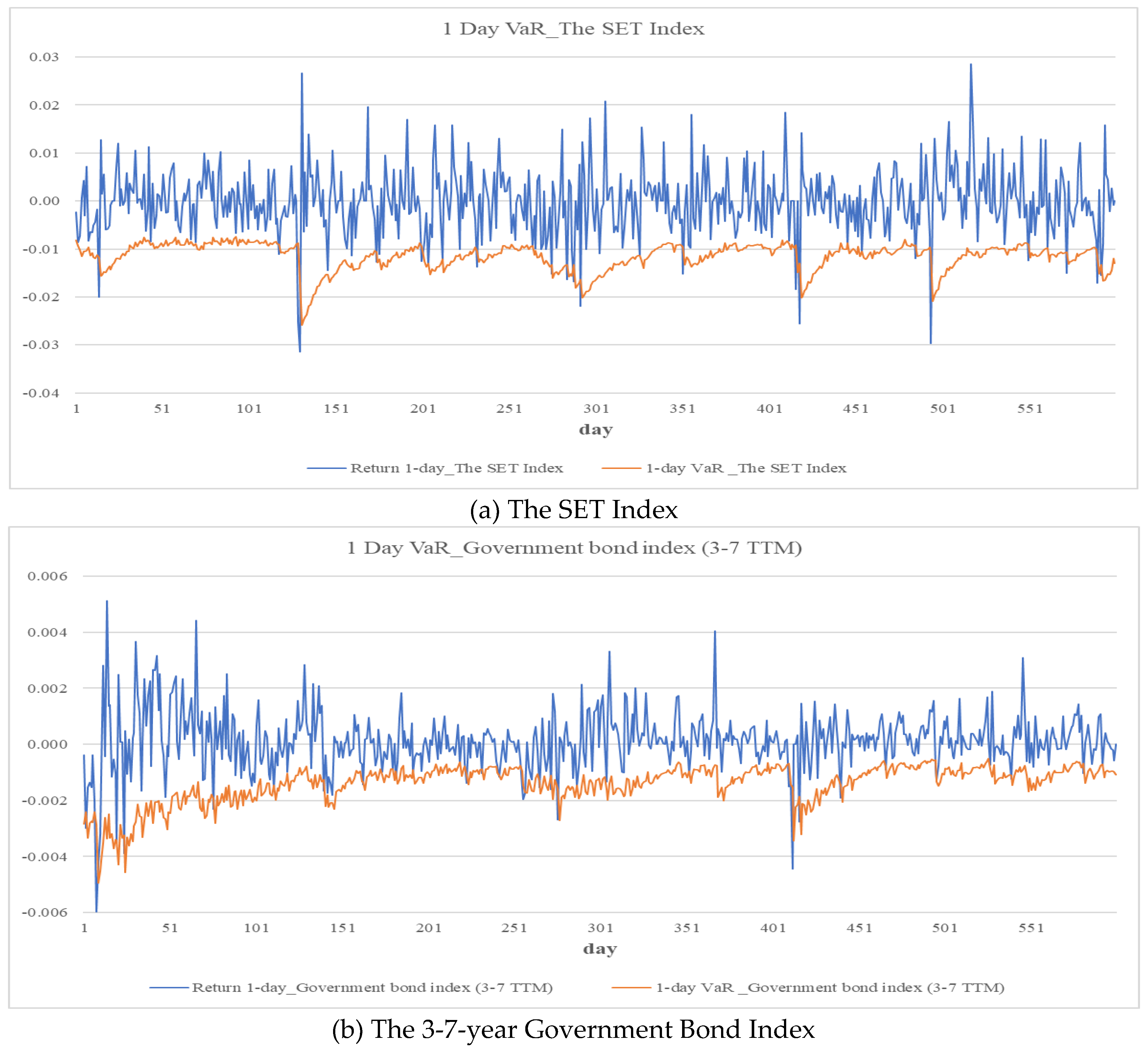
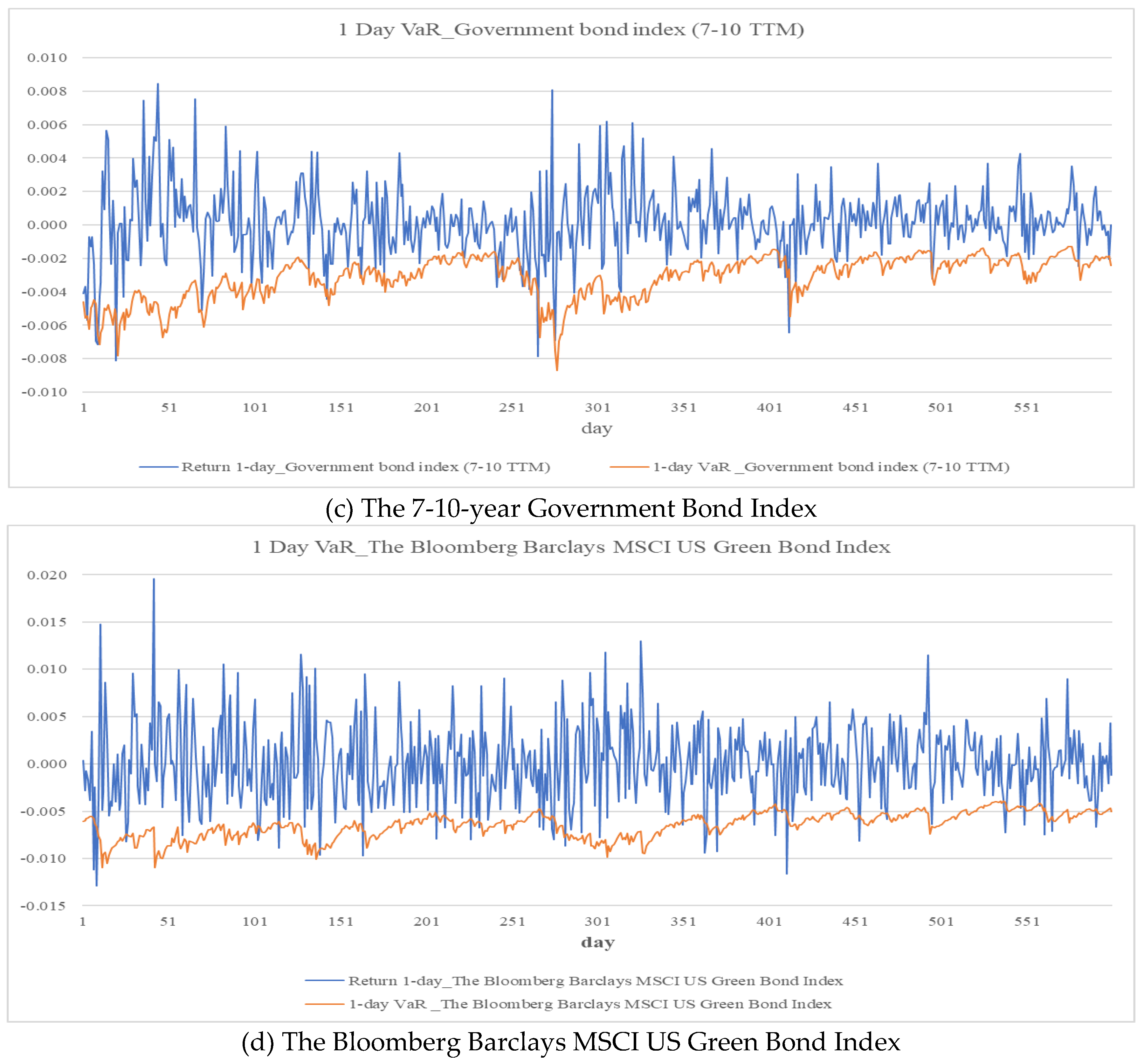
Figure 2.
10-day-ahead VaR forecasting of (a) The SET Index; (b) The 3-7-year Government Bond Index; (c) The 7-10-year Government Bond Index; (d) The Bloomberg Barclays MSCI US Green Bond Index.
Figure 2.
10-day-ahead VaR forecasting of (a) The SET Index; (b) The 3-7-year Government Bond Index; (c) The 7-10-year Government Bond Index; (d) The Bloomberg Barclays MSCI US Green Bond Index.
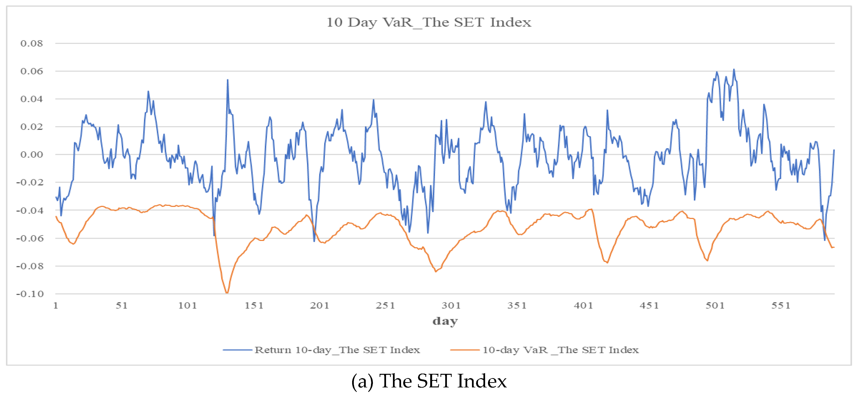
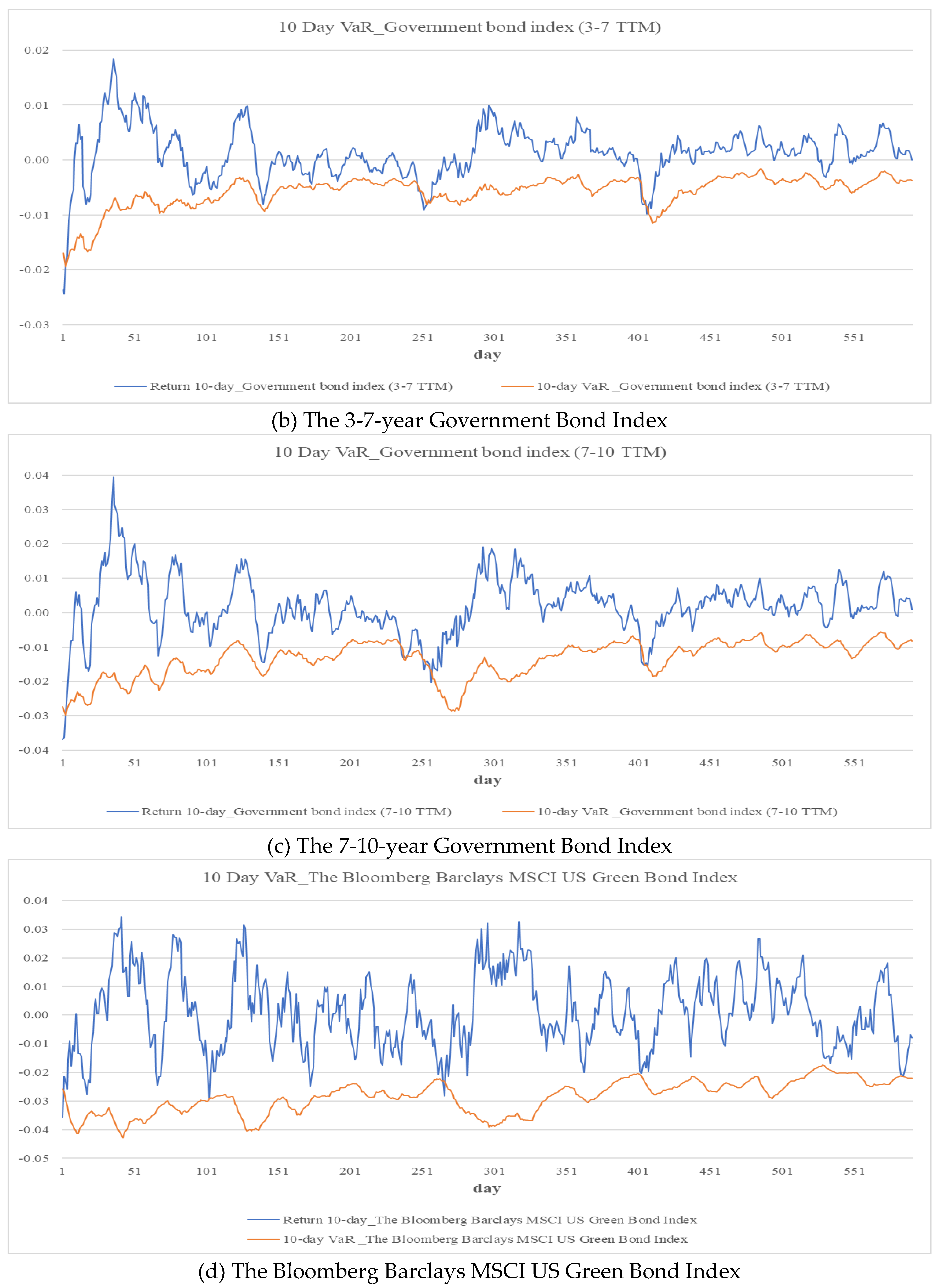
Figure 3.
One-day-ahead EVT VaR forecasting of (a) The SET Index; (b) The 3-7-year Government Bond Index; (c) The 7-10-year Government Bond Index); (d) The Bloomberg Barclays MSCI US Green Bond Index .
Figure 3.
One-day-ahead EVT VaR forecasting of (a) The SET Index; (b) The 3-7-year Government Bond Index; (c) The 7-10-year Government Bond Index); (d) The Bloomberg Barclays MSCI US Green Bond Index .
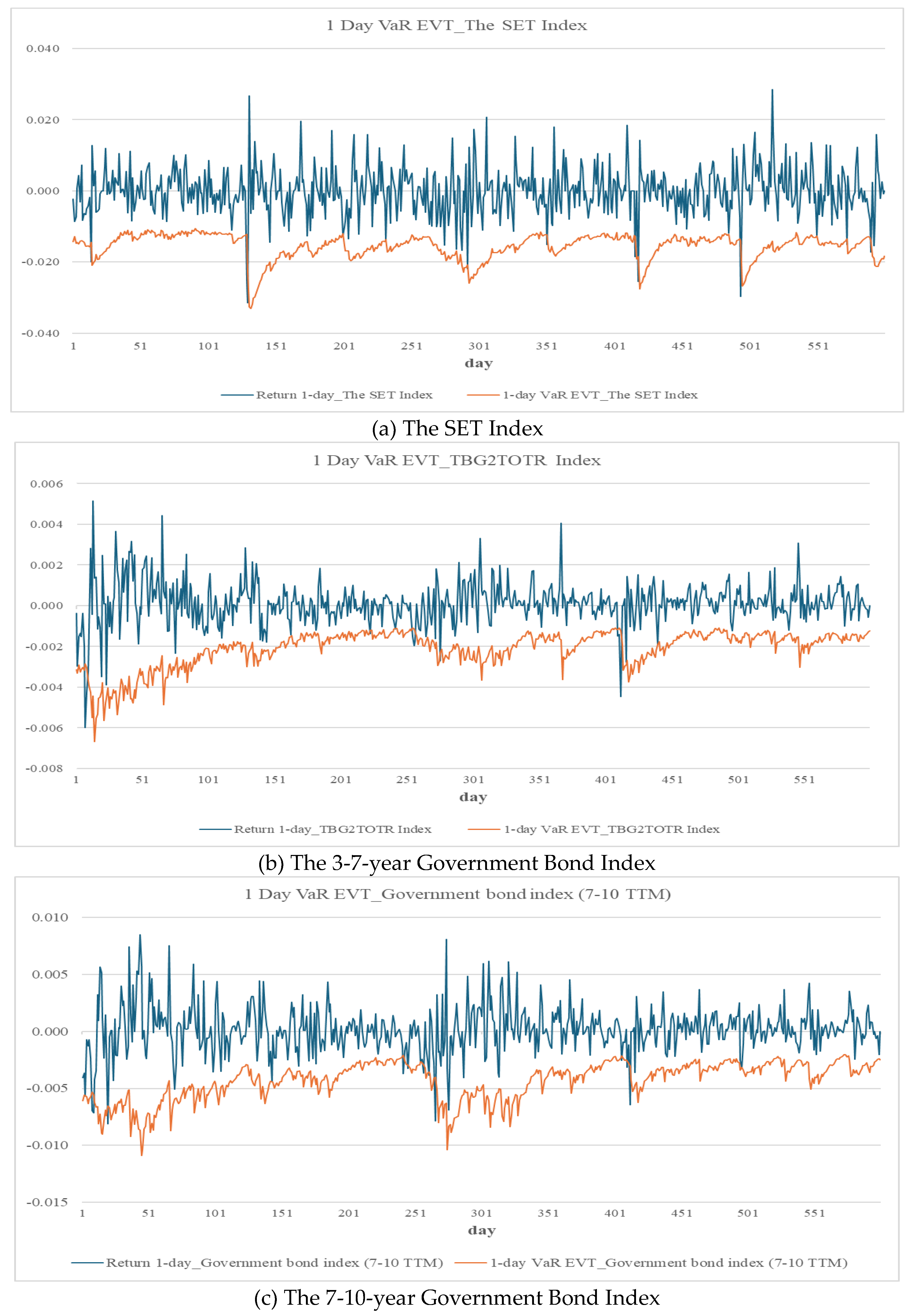
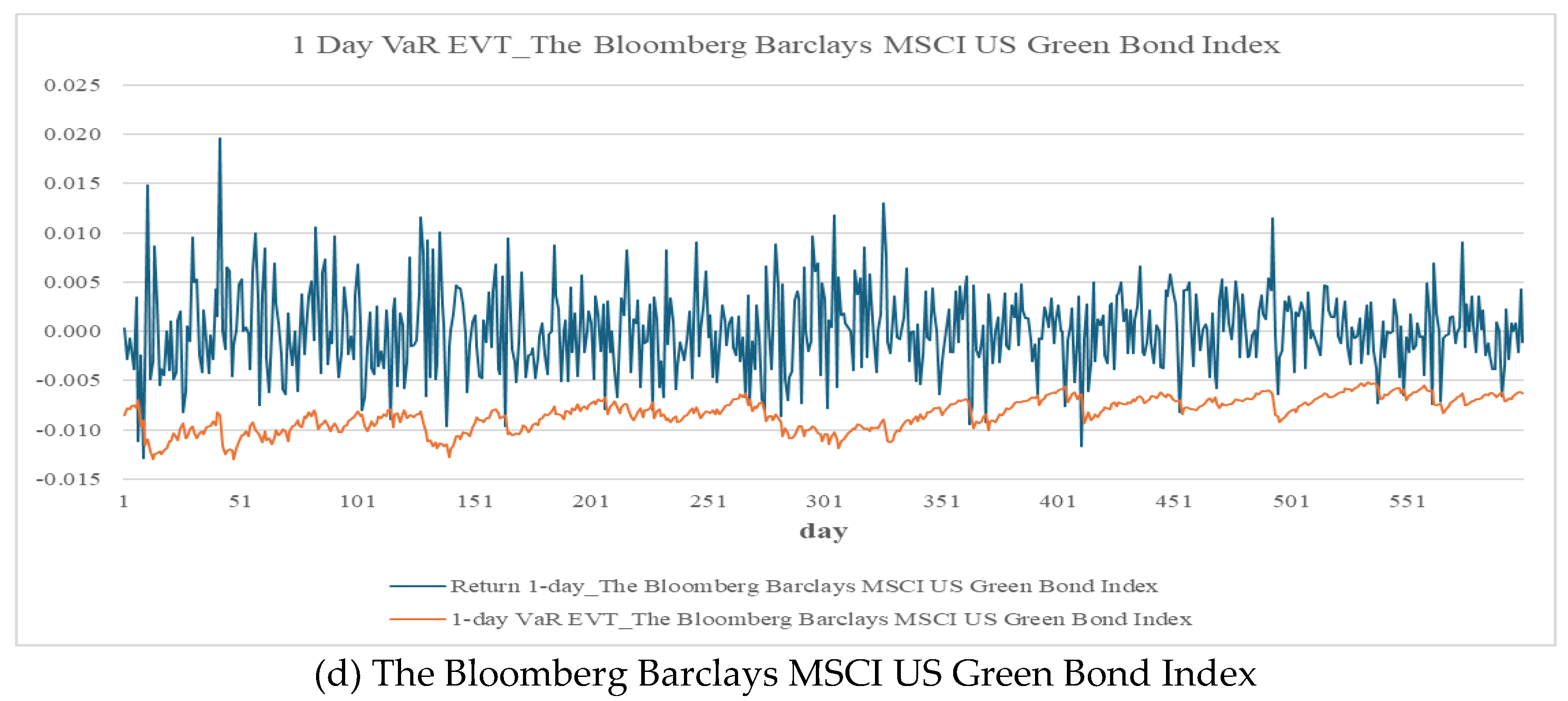

Table 1.
Summary statistics for eight assets.
| SET Index | Dubai Crude Oil | Thai Bullion Gold | 3-7 TTM GOV | 7-10 TTM GOV | JPY/THB Exchange Rate | Property Sector Index | Bloomberg Barclays MSCI US Green Bond Index | |
|---|---|---|---|---|---|---|---|---|
| Mean | 0.00015 | -0.00012 | 0.00028 | 0.00011 | 0.00015 | -0.00012 | 0.00007 | 0.00007 |
| Median | 0.00000 | 0.00050 | 0.00003 | 0.00011 | 0.00013 | -0.00017 | 0.00000 | 0.00005 |
| Maximum | 0.07656 | 0.18789 | 0.04715 | 0.00859 | 0.01651 | 0.04207 | 0.08322 | 0.01957 |
| Minimum | -0.11384 | -0.31530 | -0.05498 | -0.00947 | -0.01768 | -0.03333 | -0.14303 | -0.02087 |
| SD | 0.00878 | 0.02492 | 0.00846 | 0.00107 | 0.00230 | 0.00554 | 0.01126 | 0.00286 |
| Skewness | -1.606 | -0.748 | -0.045 | -0.509 | -0.366 | 0.238 | -1.351 | -0.203 |
| Kurtosis | 24.820 | 13.871 | 3.079 | 10.091 | 6.154 | 4.741 | 20.541 | 4.413 |
| JB | 58,149.93 | 14,393.36 | 1.71 | 6,134.58 | 1,253.54 | 389.60 | 3,7656.12 | 258.45 |
| JB (p-value) | 0.000 | 0.000 | 0.427 | 0.000 | 0.000 | 0.000 | 0.000 | 0.000 |
| ADF | -13.10 | -13.41 | -13.54 | -11.66 | -12.02 | -14.61 | -13.42 | -13.37 |
| ADF (p-value) | 0.000 | 0.000 | 0.000 | 0.000 | 0.000 | 0.000 | 0.000 | 0.000 |
Table 2.
Parameter estimation results of the ARMA-GJR-GARCH model (with skewed Student-t distribution).
Table 2.
Parameter estimation results of the ARMA-GJR-GARCH model (with skewed Student-t distribution).
| Model | SET Index | Dubai Crude Oil | Thai Bullion Gold | 3-7 TTM GOV | 7-10 TTM GOV | JPY/THB Exchange Rate | Property Sector Index | Bloomberg Barclays MSCI US Green Bond Index |
|---|---|---|---|---|---|---|---|---|
| Mu (p-value) |
1.45E-04 (0.3180) |
-3.75E-06 (0.7511) |
1.25E-04 (0.3861) |
1.13E-04 (0.0000***) |
1.13E-04 (0.0003***) |
-1.08E-04 (0.2746) |
-6.00E-05 (0.0000***) |
1.06E-04 (0.0064***) |
| ar(1) (p-value) |
-0.3985 (0.0000***) |
-0.3621 (0.0000***) |
-0.0863 (0.0000***) |
0.6992 (0.0000***) |
0.1954 (0.0000***) |
-0.9976 (0.0000***) |
0.0680 (0.0000***) |
-0.0637 (0.0027***) |
| ar(2) (p-value) |
0.2656 (0.0000***) |
-1.0109 (0.0000***) |
-0.9695 (0.0000***) |
0.0599 (0.0000***) |
||||
| ar(3) (p-value) |
0.9411 (0.0000***) |
-0.0531 (0.0000***) |
0.2143 (0.0000***) |
0.9025 (0.0000***) |
||||
| ar(4) (p-value) |
0.0157 (0.0000***) |
|||||||
| ar(5) (p-value) |
-0.0527 (0.0000***) |
|||||||
| ma(1) (p-value) |
0.4124 (0.0000***) |
0.3101 (0.0000***) |
-0.4425 (0.0021***) |
0.9944 (0.0021***) |
-0.0852 (0.0000***) |
|||
| ma(2) (p-value) |
-0.2468 (0.0000***) |
1.0071 (0.0000***) |
0.8271 (0.0000***) |
-0.0263 (0.0000***) |
||||
| ma(3) (p-value) |
-0.9351 (0.0000***) |
-0.8970 (0.0000***) |
||||||
| omega (p-value) |
8.81E-07 (0.0800*) |
5.99E-06 (0.0242**) |
9.62E-07 (0.0650*) |
8.42E-09 (0.9801) | 6.84E-08 (0.8500) | 9.40E-07 (0.4100) |
3.00E-06 (0.0672*) |
9.87E-08 (0.7638) |
| alpha1 (p-value) |
0.0155 (0.0039***) |
0.0709 (0.0000***) |
0.0669 (0.0000***) | 0.0673 (0.0002***) | 0.1357 (0.0000***) | 0.0987 (0.0010***) | 0.0177 (0.0010***) | 0.069050 (0.0000***) |
| beta1 (p-value) |
0.9201 (0.0000***) |
0.8922 (0.0000***) |
0.9417 (0.0000***) | 0.9186 (0.0000***) | 0.8857 (0.0000***) | 0.8980 (0.0000***) | 0.9065 (0.0000***) | 0.918404 (0.0000***) |
| gamma 1 | 0.1087 (0.0000***) |
0.0742 (0.0012***) |
-0.0408 (0.0024***) | -0.0054 (0.6760) | -0.0451 (0.0447**) | -0.0594 (0.0049***) | 0.0858 (0.0049***) | -0.0091 (0.5132) |
| skew | 0.9074 (0.0000***) |
0.8939 (0.0000***) |
1.0267 (0.0000***) |
0.9698 (0.0000***) |
0.9922 (0.0000***) |
1.0269 (0.0000***) |
0.9167 (0.0000***) |
0.9103 (0.0000***) |
| shape | 4.5028 (0.0000***) |
4.7935 (0.0000***) |
4.9194 (0.0000***) | 4.6552 (0.0000***) | 4.0896 (0.0000***) | 5.6768 (0.0000***) | 4.6055 (0.0000***) | 6.8252 (0.0000***) |
| AIC | -7.0677 | -4.9339 | -6.8785 | -11.391 | -9.6517 | -7.7985 | -6.5029 | -9.4954 |
| Ljung-Box Test (p-value) |
6.6342 (0.2318) |
1.4770 (0.9574) |
1.8907 (0.9176) |
1.0713 (0.9831) |
1.4362 (0.9606) |
1.4830 (0.9570) |
10.3583 (0.0420**) |
2.5347 (0.8326) |
| ARCH LM Test (p-value) |
7.2680 (0.07601) |
1.5889 (0.8034) |
1.9305 (0.7320) |
1.3349 (0.8538) |
1.0280 (0.9089) |
0.0899 (0.9995) |
12.6000 (0.0045***) |
1.6175 (0.7975) |
Note: *** significant at 0.01, ** significant at 0.05, * significant at 0.1.
Table 3.
Parameter estimation results of the ARMA-GJR-GARCH-EVT model.
| u | Nu | AIC | (Lower, Upper) | Standard | (Lower, Upper) | Standard | Distribution | KS Test | |
|---|---|---|---|---|---|---|---|---|---|
| SET Index ARMA(3,3)-GJR-GARCH(1,1) |
1.4735 | 159 | 223.150 | 0.6838 (0.5382, 0.8295) |
0.0743 | 0.0755 (-0.0716, 0.2216) |
0.0745 | exponential | 0.4553 |
| Dubai Crude Oil ARMA(3,2)-GJR-GARCH(1,1) |
1.4096 | 159 | 227.495 | 0.6464 (0.4938, 0.7990) |
0.07779 | 0.1454 (-0.0337, 0.3245) |
0.0914 | exponential | 0.9946 |
| Thai Bullion Gold ARMA(1,0)-GJR-GARCH(1,1) |
1.3811 | 159 | 161.983 | 0.5389 (0.4060, 0.6718) |
0.0678 | 0.1213 (-0.0712, 0.3138) |
0.0982 | exponential | 0.6723 |
| 3-7 TTM GOV ARMA(3,2)-GJR-GARCH(1,1) |
1.4691 | 159 | 243.778 | 0.6979 (0.5128, 0.8829) |
0.0944 | 0.1200 (-0.0957, 0.3357) |
0.1101 | exponential | 0.3579 |
| 7-10 TTM GOV ARMA(1,0)-GJR-GARCH(1,1) |
1.3433 | 159 | 211.324 | 0.7825 (0.6090, 0.9560) |
0.0885 | -0.0965 (-0.2553, 0.0624) |
0.0810 | exponential | 0.8511 |
| JPY/THB Exchange Rate ARMA(1,1)-GJR-GARCH(1,1) |
1.3525 | 159 | 156.536 | 0.5445 (0.4181, 0.6710) |
0.0645 | 0.0938 (-0.0794, 0.2670) |
0.0884 | exponential | 0.9075 |
| Property Sector Index ARMA(5,3)-GJR-GARCH(1,1) |
1.3803 | 159 | 234.215 | 0.6320 (0.4805, 0.7835) |
0.0773 | 0.1891 (0.0042, 0.3739) |
0.0943 | pareto | 0.9991 |
| Bloomberg Barclays MSCI US Green Bond Index ARMA(1,0)-GJR-GARCH(1,1) |
1.4300 | 159 | 181.911 | 0.6146 (0.4806, 0.7485) |
0.0683 | 0.0526 (-0.1003, 0.2056) |
0.0780 | exponential | 0.9475 |
Table 4.
R-vine copula estimation for life insurers.
| D-vine copula estimation for the five-asset portfolio | |||||||||||
| Copula | Edge | Parameter 1 | Parameter 2 | Tau | Lower Tail | Upper Tail | |||||
| Tree 1 | t | 1,3 | 0.98 | 19.96 | 0.87 | 0.64 | 0.64 | ||||
| t | 2,4 | 0.82 | 10.59 | 0.62 | 0.31 | 0.31 | |||||
| t | 5,1 | -0.91 | 8.91 | -0.72 | 0.00 | 0.00 | |||||
| t | 5,2 | 0.95 | 3.38 | 0.80 | 0.75 | 0.75 | |||||
| Tree 2 | t | 5,3|1 | -0.65 | 7.55 | -0.45 | 0.00 | 0.00 | ||||
| t | 5,4|2 | 0.46 | 5.83 | 0.31 | 0.16 | 0.16 | |||||
| t | 2,1|5 | -0.03 | 30.00 | - 0.02 | 0.00 | 0.00 | |||||
| Tree 3 | t | 2,3|5,1 | -0.32 | 13.77 | -0.20 | 0.00 | 0.00 | ||||
| t | 1,4|5,2 | -0.79 | 7.20 | -0.58 | 0.00 | 0.00 | |||||
| Tree 4 | t | 4,3|2,5,1 | 0.14 | 18.69 | 0.09 | 0.00 | 0.00 | ||||
| Log-likelihood | 7,733.54 | ||||||||||
| AIC | -15,427.08 | ||||||||||
| BIC | -15,312.54 | ||||||||||
| D-vine copula estimation for the six-asset portfolio | |||||||||||
| Copula | Edge | Parameter1 | Parameter2 | Tau | Lower Tail | Upper Tail | |||||
| Tree 1 | t | 1,3 | 0.98 | 19.96 | 0.87 | 0.64 | 0.64 | ||||
| t | 2,4 | 0.82 | 10.59 | 0.62 | 0.31 | 0.31 | |||||
| t | 5,1 | -0.91 | 8.91 | -0.72 | 0.00 | 0.00 | |||||
| t | 6,2 | 0.93 | 6.04 | 0.75 | 0.62 | 0.62 | |||||
| t | 6,5 | 0.92 | 8.99 | 0.74 | 0.53 | 0.53 | |||||
| Tree 2 | t | 5,3|1 | -0.65 | 7.55 | -0.45 | 0.00 | 0.00 | ||||
| t | 6,4|2 | -0.32 | 10.62 | -0.21 | 0.00 | 0.00 | |||||
| t | 6,1|5 | 0.50 | 8.08 | 0.34 | 0.12 | 0.12 | |||||
| t | 5,2|6 | 0.67 | 5.15 | 0.47 | 0.31 | 0.31 | |||||
| Tree 3 | t | 6,3|5,1 | -0.38 | 15.69 | -0.25 | 0.00 | 0.00 | ||||
| t | 5,4|6,2 | 0.61 | 5.40 | 0.42 | 0.26 | 0.26 | |||||
| t | 2,1|6,5 | -0.29 | 13.39 | -0.18 | 0.00 | 0.00 | |||||
| Tree 4 | t | 2,3|6,5,1 | -0.14 | 23.76 | -0.09 | 0.00 | 0.00 | ||||
| t | 1,4|5,6,2 | -0.69 | 8.01 | -0.49 | 0.00 | 0.00 | |||||
| Tree 5 | t | 4,3|2,6,5,1 | 0.09 | 19.54 | 0.06 | 0.00 | 0.00 | ||||
| Log-likelihood | 9,545.86 | ||||||||||
| AIC | -19,031.73 | ||||||||||
| BIC | -18,859.92 | ||||||||||
Table 5.
Optimal portfolio weights based on Sharpe ratio maximization for life insurers.
| Optimal portfolio weights based on Sharpe ratio maximization for the five-asset portfolio | ||||||||||
| Asset | SET Index | Thai Bullion Gold | Property Sector Index | 7-10 TTM GOV | JPY/THB Exchange Rate | |||||
| Weight | 0.30 | 0.05 | 0.05 | 0.50 | 0.10 | |||||
| Optimal portfolio weights based on Sharpe ratio maximization for the six-asset portfolio | ||||||||||
| Asset | SET Index | Thai Bullion Gold | Property Sector Index | 7-10 TTM GOV | JPY/THB Exchange Rate | Bloomberg Barclays MSCI US Green Bond Index | ||||
| Weight | 0.20 | 0.05 | 0.10 | 0.50 | 0.05 | 0.10 | ||||
Table 6.
R-vine copula estimation for non-life insurers.
| D-vine copula estimation for the five-asset portfolio | |||||||||||
| Copula | Edge | Parameter 1 | Parameter 2 | Tau | Lower Tail | Upper Tail | |||||
| Tree 1 | t | 1,3 | 0.98 | 20.16 | 0.87 | 0.64 | 0.64 | ||||
| t | 2,4 | -0.82 | 12.52 | -0.61 | 0.00 | 0.00 | |||||
| t | 5,1 | -0.91 | 8.93 | -0.72 | 0.00 | 0.00 | |||||
| t | 5,2 | -0.97 | 3.95 | -0.83 | 0.00 | 0.00 | |||||
| Tree 2 | t | 5,3|1 | -0.65 | 7.55 | -0.45 | 0.00 | 0.00 | ||||
| t | 5,4|2 | 0.16 | 12.37 | 0.11 | 0.01 | 0.01 | |||||
| t | 2,1|5 | 0.32 | 14.47 | -0.21 | 0.01 | 0.01 | |||||
| Tree 3 | t | 2,3|5,1 | 0.33 | 13.44 | 0.21 | 0.02 | 0.02 | ||||
| t | 1,4|5,2 | -0.81 | 6.31 | -0.60 | 0.00 | 0.00 | |||||
| Tree 4 | t | 4,3|2,5,1 | 0.22 | 10.50 | 0.14 | 0.00 | 0.00 | ||||
| Log-likelihood | 8,037.66 | ||||||||||
| AIC | -16,035.31 | ||||||||||
| BIC | -15,920.77 | ||||||||||
| D-vine copula estimation for the six-asset portfolio | |||||||||||
| Copula | Edge | Parameter1 | Parameter2 | Tau | Lower Tail | Upper Tail | |||||
| Tree 1 | t | 1,3 | 0.98 | 20.16 | 0.87 | 0.64 | 0.64 | ||||
| t | 5,1 | -0.91 | 8.93 | -0.72 | 0.00 | 0.00 | |||||
| t | 5,2 | -0.97 | 3.95 | -0.83 | 0.00 | 0.00 | |||||
| t | 6,4 | -0.92 | 4.71 | -0.74 | 0.00 | 0.00 | |||||
| t | 6,5 | 0.92 | 8.93 | 0.74 | 0.54 | 0.54 | |||||
| Tree 2 | t | 5,3|1 | -0.65 | 7.55 | -0.45 | 0.00 | 0.00 | ||||
| t | 2,1|5 | 0.32 | 14.47 | 0.21 | 0.01 | 0.01 | |||||
| t | 6,2|5 | -0.28 | 10.77 | -0.18 | 0.00 | 0.00 | |||||
| t | 5,4|6 | 0.24 | 15.45 | 0.15 | 0.01 | 0.01 | |||||
| Tree 3 | t | 2,3|5,1 | 0.33 | 13.44 | 0.21 | 0.02 | 0.02 | ||||
| t | 6,1|2,5 | 0.62 | 11.48 | 0.42 | 0.11 | 0.11 | |||||
| t | 4,2|6,5 | 0.07 | 30.00 | 0.05 | 0.00 | 0.00 | |||||
| Tree 4 | t | 6,3|2,5,1 | -0.26 | 26.47 | -0.17 | 0.00 | 0.00 | ||||
| t | 4,1|6,2,5 | -0.44 | 17.91 | -0.29 | 0.00 | 0.00 | |||||
| Tree 5 | t | 4,3|6,2,5,1 | 0.32 | 17.94 | 0.20 | 0.01 | 0.01 | ||||
| Log-likelihood | 9,797.16 | ||||||||||
| AIC | -19,534.31 | ||||||||||
| BIC | -19,362.50 | ||||||||||
Table 7.
Optimal portfolio weights based on Sharpe ratio maximization for non-life insurers.
| Optimal portfolio weights based on Sharpe ratio maximization for the five-asset portfolio | ||||||||||
| Asset | SET Index | Dubai Crude Oil | Property Sector Index | 7-10 TTM GOV | JPY/THB Exchange Rate | |||||
| Weight | 0.05 | 0.05 | 0.05 | 0.55 | 0.30 | |||||
| Optimal portfolio weights based on Sharpe ratio maximization for the six-asset portfolio | ||||||||||
| Asset | SET Index | Dubai Crude Oil | Property Sector Index | 7-10 TTM GOV | JPY/THB Exchange Rate | Bloomberg Barclays MSCI US Green Bond Index | ||||
| Weight | 0.10 | 0.05 | 0.05 | 0.40 | 0.30 | 0.10 | ||||
Table 8.
One-day-ahead VaR and 10-day-ahead VaR backtesting: ARMA–GJR–GARCH model (with skewed Student-t innovations) performance.
Table 8.
One-day-ahead VaR and 10-day-ahead VaR backtesting: ARMA–GJR–GARCH model (with skewed Student-t innovations) performance.
| Asset Model | SET Index ARMA(3,3)-GJR-ARCH (1,1) |
Dubai Crude Oil ARMA(3,2)-GJR-GARCH (1,1) |
Thai Bullion Gold ARMA(1,0)-GJR-GARCH (1,1) |
3-7 TTM GOV ARMA(3,2)-GJR-GARCH (1,1) |
7-10 TTM GOV ARMA(1,0)-GJR-GARCH (1,1) |
JPY/THB Exchange Rate ARMA(1,1)-GJR-GARCH (1,1) |
Property Sector Index ARMA(5,3)-GJR-GARCH (1,1) |
Bloomberg Barclays MSCI US Green Bond Index ARMA(1,0)-GJR-GARCH (1,1) |
|---|---|---|---|---|---|---|---|---|
|
Average One-day-ahead VaR at 95% |
-1.16% | -3.38% | -1.34% | -0.14% | -0.31% | -0.94% | -1.49% | -0.65% |
| Observed Exceedance Rate | 4.17% | 5.17% | 4.00% | 5.17% | 3.50% | 4.50% | 3.83% | 5.50% |
| Kupiec Test |
0.928 | 0.035 | 1.352 | 0.035 | 3.161 | 0.326 | 1.863 | 0.306 |
| Kupiec’s p-value | 0.335 | 0.852 | 0.245 | 0.852 | 0.075* | 0.568 | 0.172 | 0.580 |
| Christoffersen Test | 0.912 | 0.327 | 1.182 | 0.140 | 4.764 | 0.361 | 1.855 | 0.337 |
| Christoffersen’s p-value | 0.634 | 0.849 | 0.554 | 0.932 | 0.092* | 0.835 | 0.395 | 0.845 |
| Average 10-day-ahead VaR at 99% | -5.19% | -14.93% | -5.92% | -0.58% | -1.34% | -4.29% | -6.70% | -2.86% |
| Observed Exceedance Rate | 0.85% | 0.17% | 0.85% | 2.03% | 1.52% | 0.51% | 0.68% | 0.68% |
| Kupiec Test |
0.149 | 6.308 | 0.149 | 4.882 | 1.407 | 1.766 | 0.703 | 0.703 |
| Kupiec’s p-value | 0.699 | 0.012** | 0.699 | 0.027** | 0.236 | 0.184 | 0.402 | 0.402 |
| Christoffersen Test | 4.035 | 4.958 | 3.594 | 3.546 | 0.960 | 4.958 | 4.035 | 5.452 |
| Christoffersen’s p-value | 0.133 | 0.084* | 0.139 | 0.170 | 0.618 | 0.084* | 0.133 | 0.065* |
Note: ** significant at 0.05, * significant at 0.1.
Table 9.
One-day-ahead VaR backtesting: ARMA–GJR–GARCH-EVT model performance.
| Asset Model | SET Index ARMA(3,3)-GJR-ARCH (1,1) |
Dubai Crude Oil ARMA(3,2)-GJR-GARCH (1,1) |
Thai Bullion Gold ARMA(1,0)-GJR-GARCH (1,1) |
3-7 TTM GOV ARMA(3,2)-GJR-GARCH (1,1) |
7-10 TTM GOV ARMA(1,0)-GJR-GARCH (1,1) |
JPY/THB Exchange Rate ARMA(1,1)-GJR-GARCH (1,1) |
Property Sector Index ARMA(5,3)-GJR-GARCH (1,1) |
Bloomberg Barclays MSCI US Green Bond Index ARMA(1,0)-GJR-GARCH (1,1) |
|---|---|---|---|---|---|---|---|---|
| Average One-day-ahead VaR at 97.5% | -1.56% | -4.46% | -1.64% | -0.21% | -0.43% | -1.09% | -1.91% | -0.84% |
| Observed Exceedance Rate | 2.00% | 2.00% | 2.67% | 2.00% | 2.33% | 3.67% | 1.83% | 2.83% |
| Kupiec | 0.660 | 0.660 | 0.067 | 0.660 | 0.070 | 2.936 | 1.204 | 0.262 |
| Test | 0.417 | 0.417 | 0.796 | 0.417 | 0.791 | 0.087* | 0.273 | 0.609 |
| Kupiec’s p-value | 2.809 | 1.989 | 0.612 | 6.608 | 1.359 | 2.389 | 3.838 | 2.605 |
| Christoffersen Test | 0.245 | 0.370 | 0.736 | 0.037** | 0.507 | 0.303 | 0.147 | 0.272 |
Note: ** significant at 0.05, * significant at 0.1.
Table 10.
Performance comparison of R-vine copula models: Sharpe ratio and VaR backtesting.
| Portfolio Type | Average Sharpe Ratio |
% of Windows with Higher Sharpe Ratio | Average One-Day-Ahead VaR (95%) | % of Windows with Lower One-Day-Ahead VaR | |
|---|---|---|---|---|---|
| Life insurer portfolios | Five-Asset Portfolio | -0.0432 | 19.50% | -0.1576% | 39.67% |
| Six-Asset Portfolio | 0.0063 | 80.50% | -0.1428% | 60.33% | |
| Non- life insurer portfolios | Five-Asset Portfolio | -0.0928 | 39.33% | -0.1004% | 66.17% |
| Six-Asset Portfolio | -0.0441 | 60.67% | -0.1264% | 33.83% |
Disclaimer/Publisher’s Note: The statements, opinions and data contained in all publications are solely those of the individual author(s) and contributor(s) and not of MDPI and/or the editor(s). MDPI and/or the editor(s) disclaim responsibility for any injury to people or property resulting from any ideas, methods, instructions or products referred to in the content. |
© 2025 by the authors. Licensee MDPI, Basel, Switzerland. This article is an open access article distributed under the terms and conditions of the Creative Commons Attribution (CC BY) license (http://creativecommons.org/licenses/by/4.0/).
Copyright: This open access article is published under a Creative Commons CC BY 4.0 license, which permit the free download, distribution, and reuse, provided that the author and preprint are cited in any reuse.