
Submitted:
29 July 2025
Posted:
30 July 2025
You are already at the latest version
Abstract
Padé approximants are computational tools customarily employed for resumming divergent asymptotic Stieltjes series. However, they become ineffective or even fail when applied to Stieltjes series whose moments do not satisfy the Calerman condition. Differently from Padé, Levin-type transformations incorporate important structural information on the converging factors of a typical Stieltjes series. For example, the computational superiority of Weniger’s δ-transformation over Wynn’s epsilon algorithm is ultimately based on the fact that Stieltjes series converging factors can always be represented as inverse factorial series. In the present paper, the converging factors of an important class of superfactorially divergent asympotic Stieltjes series are investigated via an algorithm developed one year ago from the first-order difference equation satisfied by the Stieltjes series converging factors. Our analysis includes the analytical derivation of the inverse factorial representation for the moment ratio sequence of the series under investigation, and demonstrates the numerical effectiveness of our algorithm, together with its implementation ease. Moreover, a new perspective on the converging factor representation problem is also proposed, by reducing the recurrence relation to a linear Cauchy problem whose explicit solution is provided via Faà di Bruno’s formula and Bell’s polynomials.
Keywords:
mathematical physics
; divergent series
; Stieltjes series
; converging factors
MSC: 40-08; 40A05; 40A30
1. Introduction
Stieltjes series are fundamental tools in mathematical physics and continue to receive considerable attention. For instance, the, factorially divergent perturbation expansion of the energy eigenvalue of the -symmetric Hamiltonian has been proved to be Stieltjes [1,2], as conjectured ten years earlier [3]. More recently, it was shown that even the character of the celebrated Bessel solution of Kepler’s equation [4] belongs to the Stieltjes family [5].
The present paper constitutes the follow up of a previous work on the study of convergence factors of Stieltjes series [6]. A well-established general convergence theory based on Padé approximants already exists for Stieltjes series. For example, if the moment sequence of a given Stieltjes series satisfies Carleman’s condition, then sequences of its diagonal or near-diagonal Padé approximants are guaranteed to converge to the Stieltjes function that generates the series itself (see for instance Baker and Graves-Morris [7]). This has consecrated Padé approximants as the main computational tool for the resummation of Stieltjes series. However, Padé approximants are subject to intrinsic limitation, especially when dealing with wildly divergent series (e.g., such that Calerman’s condition is not satisified). This has led to the development of new types of sequence transformations for summing divergent series. Among them, Levin-type transformations [8,9,10] proved to be particularly effective and powerful, in some cases outperforming Padé-based methods, such as Wynn’s epsilon algorithm [11]. Within the last four decades, an important literature has been produced, especially on nonlinear and nonregular sequence transformations, [9,12,13,14,15,16,17,18,19,20,21,22,23,24,25,26,27,28].
About fifteen years ago, Ernst Joachim Weniger and I embarked on a challenging research project. We believed that a solid theoretical understanding of Levin-type sequence transformations – perhaps even a comprehensive convergence theory – could offer a valid alternative to Padé approximants for summing divergent Stieltjes series, particularly where Padé-based methods fail. Reference [28] demonstrated the remarkable computational effectiveness of Weniger’s -transformation [9]. This specific Levin-type transformation not only successfully resummed the celebrated Euler series (a paradigm of factorial divergence) but did it with convergence rates greater than Padé. The proof in [28] relied on an inverse factorial expansion for Euler series converging factors, discovered a few years before [29]. Factorial series are often overlooked mathematical objects, largely unknown to non-specialists. Weniger’s merits include unearthing them while developing his -transformation.
Ernst Joachim Weniger passed away on August 10th, 2022. Two years later, his contributions and legacy were celebrated in Ref. [6], where a constructive proof that converging factors of typical Stieltjes series can be expressed through inverse factorial series, was proposed. This proof was cast as an algorithm based on a first-order difference equation, which has been shown to be satisfied by the convergent factors of any Stieltjes series [6]. The present paper directly builds upon that tribute, providing a significant continuation of our work. Specifically, the algorithm proposed in [6] is here tested on a class of Stieltjes series with superfactorial moment growths. Weniger’s -transformation has previously succeeded in resumming extremely divergent perturbation expansions, closely related to this class of Stieltjes series [30,31,32,33]. In some of these cases, Padé approximants often proved to be ineffective, as seen with the Rayleigh-Schrödinger perturbation series for the sextic anharmonic oscillator, or even failed in the more challenging octic case [34].
In Section 2, the main definitions and properties of Stieltjes series and Stieltjes functions are briefly reviewed, together with a resume of Ref. [6]. In Section 3, the class of superfactorially divergent series is presented, and the inverse factorial representation of the moment ratio sequence is analytically found. Section 4 illustrates some examples of application of our algorithm, to show its effectiveness and its ease of implementation. Finally, in Section 5 the converging factor representation problem is reformulated from a different perspective, by transforming the recurrence relation of [6] into a linear Cauchy’s problem, whose explicit solution is obtained using Faà di Bruno’s formula, together with the use of Bell’s polynomials [35] (Section 3.3).
For an improved readability, the most technical parts have been relegated to appendices.
2. Stieltjes Series Converging Factors, Factorial Series, and the Moment Problem
Consider a nondecreasing, real-valued function defined for , possessing infinitely many points of increase. This ensures that the associated measure, say , is positive on . It will be assumed that all of its moments, defined as:
are finite. The formal power series
is called a Stieltjes series. Such series turns out to be asymptotic, in the sense of Poincaré, for , to the function defined by
which is analytic in the complex plane cut along the negative real axis (i.e., , and is called Stieltjes function.
The probably most known example of Stieltjes series is the Euler series [36], characterized by the moment sequence , and asymptotic to the Euler integral,
which has the form given in Eq. (3), with the measure .
Given a sequence of moments , is the corresponding Stieltjes function uniquely determined? And, if so, is it possible to decode the asymptotic series into Eq. (2) to retrieve the correct value of F? The solution of such fundamental problem, which is known as the Stieltjes moment problem, depends on the growth rate of the moments. Carleman’s condition represents an important sufficient criterion to assess unicity to the moment problem. In particular, the Stieltjes moment problem is determinate if the series
diverges.
Any Stieltjes function can be expressed as the sum of the nth-order partial sum of the associated asympotic series (2) and of a truncation error which has itself the form of a Stieltjes integral (see for example [9] (Theorem 13-1)). More precisely, we have
and the truncation error term can always be recast as follows:
where the function
will be called the mth-order converging factor [37,38].1
From Eq. (7), it appears that, if reasonable estimates of the converging factor could be achieved without resorting to the numerical evaluation of the integral into Eq. (8), then the numerical evaluation of via its asymptotics would be in principle possible. The search of techniques aimed at estimating convergence factors plays a role of pivotal importance to decode divergent asymptotic series. In [6] it has been shown that, given a Stieltjes series, the converging factor in Eq. (8) can always be represented as an inverse factorial series. Our proof was ultimately based on (i) the fact that must satisfy the following first-order difference equation [6]:
and (ii) that inverse factorial series constitute natural tools for solving difference equations, similarly as inverse power series are used to solve differential equations. For reader’s convenience, the basic definitions and properties of factorial series will now be briefly recalled, although extensive reviews can be found, for instance, in [6,28]. More interested and motivated readers are encouraged to go through the Weniger paper [25], where a hystorical account of his re-discovery of factorial series can be found, together with a list of their most important computational features. For the scopes of the present paper, it is sufficient to limit ourselves to the following key points:
- (i)
- Let be a complex function of a complex variable x. A factorial series representation of is an expansion of the following type:where the symbol denotes the Pochhammer symbol. In the following, it will be assumed .
- (ii)
-
Compared to inverse power series, factorial series often possess superior convergence properties. For example, consider the divergent sequence and construct the following two infinite series:andThe power series diverges for all , whereas the factorial series converges for all . In other words, it may happen that a given function possessing a representation in terms of a divergent asymptotic series, also possesses a representation as a convergent factorial series.
- (iii)
-
Factorial series admit useful integral representations. Starting fromand on inserting into Eq. (10), after interchanging integration and summation, the following integral representation is found [41] (Sec. I on p. 244):where the function turns out to beNote that the function can be thought of as a truncated Mellin transform of the function , in terms of which the expanding coefficients into Eq. (10) take on the following form:where the symbol denotes the kth-order derivative of the function . In other words, is nothing but the generating function of the sequence .
The main results of the algorithm derived in Ref. [6] will now be briefly recalled. The idea consisted in searching the solution of the difference equation (9) in the form of the following inverse factorial series:
where is a real nonnegative parameter, and denotes a sequence which is independent of m. For the sake of simplicity, it will be assumed henceforth. What has been found in Ref. [6] is that the expanding coefficients ’s can be obtained in a very easy way if the moment ratio sequence admits itself an inverse factorial expansion, i.e.,
In particular, the following recurrence relation holds [6]:
where the sequence is given by
or, equivalently, by
In Ref. [6], Eqs. (20) - (23) have been applied to re-derive and further generalize (to any ) the result found in [29] as far as the converging factor of the Euler series is concerned. In the next section, they will be employed to find the inverse factorial series representation of the converging factor of an important class of superfactorial divergent Stieltjes series, which can be thought as an important suitable generalization of the Euler series.
3. A Class of Superfactorially Divergent Stieltjes Series
The class of Stieltjes series under investigation are characterized by the following moment sequence:
where and . Euler series corresponds to the choice . Asymptotic series of Eq. (24) play a role of pivotal importance in theoretical as well as mathematical physics. They are strictly related to the theory of quantum anharmonic oscillators. In two seminal papers, Bender and Wu [42,43] shown that the Rayleigh-Schrödinger perturbative expansion of the energy levels of the Hamiltonian
with , is asymptotically dominated by the Stieltjes series in Eq. (24), with . The summability of such asymptotic series has also been addressed in 1993 by Weniger et al. [33] through a series of important numerical experiments, aimed at comparing the retrieving performances of Levin’s type nonlinear transformations with those of Padé approximants, as far as the computation of the energy levels of quartic, sextic, and octic oscillators was concerned. In particular, they also considered the numerical resummation of Stieltjes series of the type into Eq. (24) for and for some integer values of . In particular, it was found that both Levin’s and Weniger’s transformations were able to decode correctly the series when , whereas Padé approximants failed to achieve the task already for , i.e., when the Calerman condition in Eq. (5) is not satisfied.
In the present section, the estimation of the converging factor of the Stieltjes series of Eq. (24) will be obtained on applying the algorithm of [6]. Our analysis will be carried out for any values of and q, while it will be set in all subsequent calculations, as said above. In order for the algorithm in Section 2 to be applied, it is mandatory to find the inverse factorial expantion of the moment ratio sequence for the class of Stieltjes series defined by Eq. (24), which can be recast as follows:
On expanding the right side of Eq. (26) as a sum of partial fraction of the form
it is not difficult to prove that (see Appendix A)
The subsequent step consists in using Waring’s formula [41] (Eq. (3) on p. 77), namely
which, together with Eqs. (27) and (28), after some algebra leads to Eq. (20) with the following expanding coefficient sequence (see Appendix B):
It should be noted how the mathematical structure of the right side of Eq. (30) is nothing but the th-order forward difference of the kth-degree polynomial , i.e.,
where the forward difference operator is defined as . In particular, since is a kth-order polynomial, it follows at once that:
The above result can be easily extended to deal with the most general inverse factorial expansion of the moment ratio. In fact, it is not difficult to show that, in order to deal with , it is sufficient to recast Eq. (26) as follows:
and then to proceed similarly as we did for the case . The final result, which is given without proof, is the following:
with the expanding coefficient sequence being now given by
4. Numerical Results
In the present section, a few examples concerning the numerical estimation of the converging factors of some of the divergent superfactorial Stieltjes series analyzed in the previous section, will be presented. Our attention will be directed to a series of important numerical experiments carried out in 1993 by Weniger et al. [33]. In particular, our computational targets are two Stieltjes integrals, namely2
and
It is not difficult to show that both integrals into Eqs. (36) and (37) can be recast in the form of Eq. (3). For the first integral, it is sufficiente to change the integration variable from t to and to let , so to have
where the measure is given by
and gives at once
corresponding to the pair in the model given into Eq. (24). More importantly, the mth-order converging factor can be analytically evaluated for any in terms of hypergeometric functions,3
Similar results hold also for the Stieltjes integral , which can be recast as
where now and
so that
corresponding to in the model given into Eq. (24). Similarly as happened for , also the converging factor of can be found exactly, although the resulting expression is quite complicated and annoying.
Our algorithm will now be tested starting from , by focusing the attention on the relative error obtained when the mth-order converging factor into Eq. (41) is going to be evaluated through the following truncated inverse factorial series:
Figure 1 shows the behaviour of the relative error, defined as
related to the converging factor defined by Eq. (41), as far as the integral is concerned, for (dashed curve), (dotted curve), and (solid curve).
It can be appreciated how the inverse factorial series representation of appears to converge as , with a convergence rate becoming larger and larger on increasing the order m, as it might be expected from Eq. (3) and from the general considerations about inverse factorial series recalled at the beginning of Section 2.
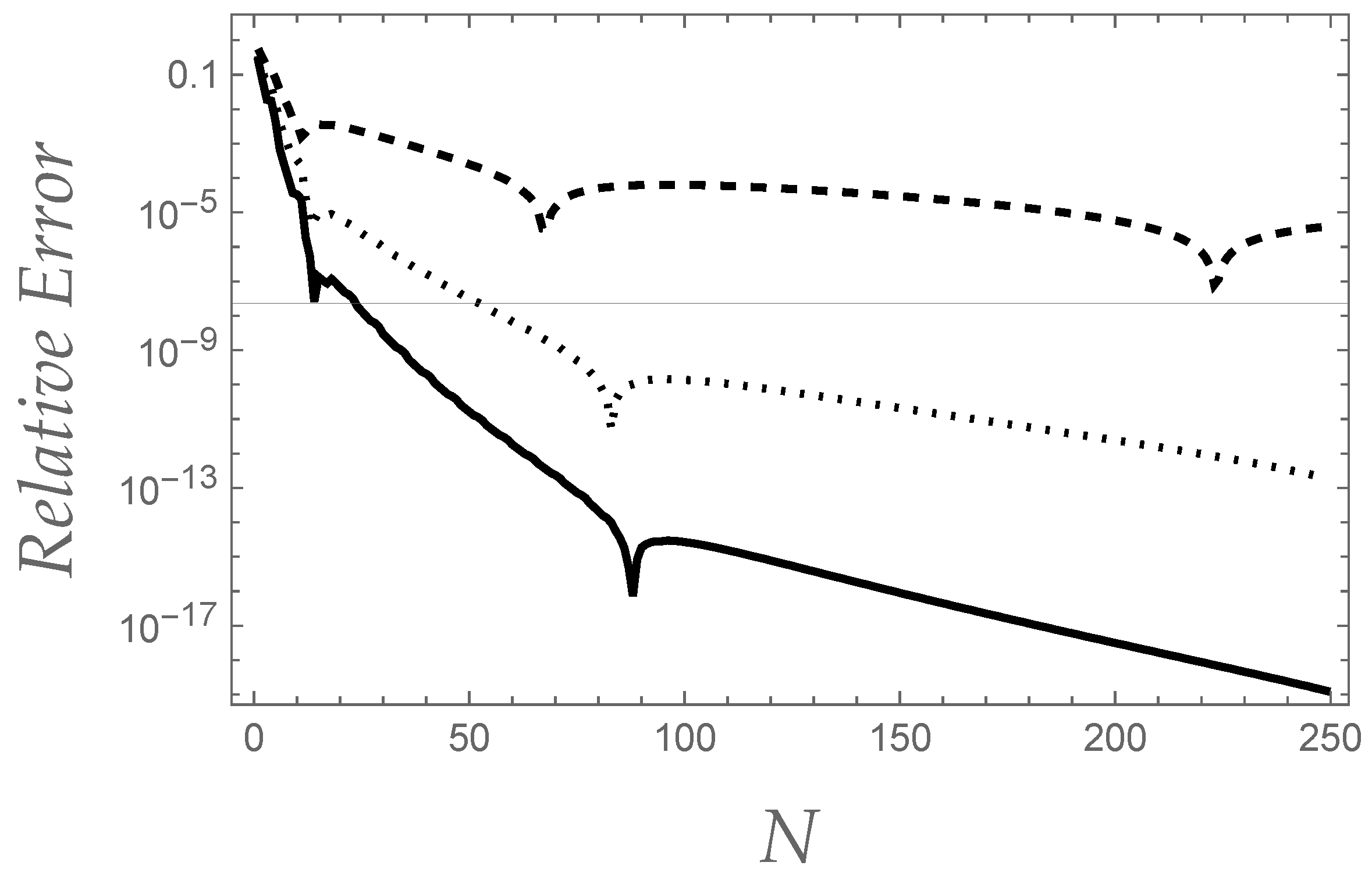
Even more interesting are the numerical results obtained as far as the estimate of the converging factor of the Stieltjes integral is concerned, which are shown in Figure 2.
In particular, it should be noted how, for both cases, the performances of our algorithm (e.g., for what concerns the order of magnitude of the relative error as a function of the factorial series truncation order) are comparable, despite the fact that choosing or determines or not the validity of Calerman’s condition, respectively. As it was put into evidence in Ref. [33], such a circumstance greatly influenced the numerical performances of Padé approximants in retrieving the correct values of as well as , while did not affect the retrieving action of Levin’s, as well as Weniger’s transformations [33]. These preliminary results corroborate our feeling about the robustness of Levin-type transformations in resumming superfactorially divergent Stieltjes series. The final part of the present paper is aimed at exploring further properties of the key role played by of the factorial expansion of converging factors, and to give some general guidelines for future estimations of the related convergence rates.
5. On Integral Representation of the Converging Factors for
In the present section, some of the results found in Section 3 will now be re-derived in a completely different way, on employing the integral representation of factorial series of Eq. (16). We are convinced that what is going to be presented could reveal of a certain importance in future, in order for the convergence features of Levin-type nonlinear transformations in resumming superfactorially divergent Stieltjes series to be explored, similarly to what has been found for the Euler series [28]. There, the starting point of our convergence analysis was just the truncated Mellin transform representation of the Euler series converging factor, which was obtained from the results published in [29]. The same results will now be rederived within a few steps, on using the recurrence relation in Eq. (9) for the converging factor , together with Eq. (24) written for , i.e.,
so that, on taking Eq. (16) into account, the following integral equation for the generating function is obtained:
On integrating by parts the first integral, we obtain
with the superscript denoting derivation with respect to t. Finally, on substituting from Eq. (49) into Eq. (48), our integral equation is transformed into the following first-order Cauchy problem for :
whose solution is
and that leads to [28] (Eq. (5.17)).4
It is then natural to ask whether similar results could be found also for the pairs , following the same strategy. For the sake of simplicity, only the cases and will now be detailed. A conjecture, which we thought to be valid for , will be proposed as an open problem at the end of the paper.
Consider now the case . From Eq. (24) we have which, once substituted into Eq. (9), gives
that can also be recast as follows:
Similarly as done for the Euler series, to solve the difference equation the integral representation in Eq. (16) will now be used, together with the two relationships
that can be proved again via partial integration. Substitution from Eq. (54) into Eq. (53) gives the following integral equation for the function :
which leads to the Cauchy problem
On letting , straigthforward algebra transforms Eq. (56) into
whose solution is . Accordingly, we have
It is not difficult to check how, after substituting from Eq. (58) into Eq. (18), the whole sequence so generated coincides with the sequence obtained through the recursive algorithm into Eqs. (21) and (23), for any z.
The case is particularly intriguing, due to the fact that when Calerman’s condition is not satisfied and Padé approximants are no longer able to decode the associated Stieltjes series. As far as Eq. (9) is concerned, we have
which can be recast as follows:
On recalling Eqs. (54) and on taking into account that
after some algebra it is possible to show that the function must satisfy the following Cauchy problem:
that, on letting , transforms into
whose explicit solution is given by
The above results would suggest that a factorial expansion of the converging factor could be costructed also for . In particular, we conjecture that the generating function can alwasy be recast as follows:
with the function being the solution of the th-order Cauchy problem
In particular, the extraction of the sequence could be done directly through Eq. (18), without explicitly solving Eq. (66). To this end, it is sufficient to note that, thanks to Eq. (65), the sequence can be generated through
and so on, where the sequence and should be achievable via recurrenced as follows:
starting from the initial values given in Eq. (66). More importantly, Eq. (67) can be given in closed-form terms on using Faà di Bruno’s formula, as shown in Appendix C, i.e.,
where the symbol denotes the partial Bell polynomial [35] (Section 3.3).
6. Conclusions
In the present paper, we explored the converging factors for a class of Stieltjes series exhibiting superfactorial divergence using the algorithm developed in [6]. We successfully demonstrated the numerical effectiveness of the algorithm and its ease of implementation. Our algorithm proved to be robust in estimating converging factors even for series whose moments do not satisfy Carleman’s condition, where Padé approximants largely fail.
We also introduced novel theoretical perspectives on the converging factor representation problem. By reducing the recurrence relation satisfied by the converging factor to a linear Cauchy problem, we provided explicit solutions using the Faà di Bruno formula and Bell’s polynomials. This could help to develop new strategies for the theoretical exploration of Levin-type sequence transformations convergence features. In particular, the integral representations of the converging factor obtained for the class of Stieltjes series investigated here are expected to be instrumental in estimating the convergence rates of Weniger’s -transformation for these class of divergent series, similar to what has been done for the Euler series [28].
Funding
This research received no external funding
Data Availability Statement
The data presented in this study are available on request from the corresponding author.
Acknowledgments
I wish to thank Turi Maria Spinozzi for his useful comments and help.
Conflicts of Interest
The author declares no conflicts of interest.
Appendix A. Proof of Eq. (uid32)
Appendix B. Proof of Eq. (30)
Appendix C. On the Faà di Bruno Formula
Given
we are interested in evaluating
where . Faà di Bruno’s formula then gives
where the symbol denotes partial Bell polynomial. In particular, since in our case we have , and
References
- Grecchi, V.; Maioli, M.; Martinez, A. Padé summability of the cubic oscillator. J. Phys. A 2009, 42, 425208–1. [Google Scholar] [CrossRef]
- Grecchi, V.; Martinez, A. The spectrum of the cubic oscillator. Commun. Math. Phys. 2013, 319, 479–500. [Google Scholar] [CrossRef]
- Bender, C.M.; Weniger, E.J. Numerical evidence that the perturbation expansion for a non-Hermitian PT-symmetric Hamiltonian is Stieltjes. J. Math. Phys. 2001, 42, 2167–2183. [Google Scholar] [CrossRef]
- Colwell, P. Solving Kepler’s Equation Over Three Centuries; Willmann-Bell: Richmond, 1993. [Google Scholar]
- Borghi, R. On the Bessel Solution of Kepler’s Equation. Mathematics 2024, 12, 154. [Google Scholar] [CrossRef]
- Borghi, R. Factorial Series Representation of Stieltjes Series Converging Factors. Mathematics 2024, 12, 2330. [Google Scholar] [CrossRef]
- Baker, Jr., G. A.; Graves-Morris, P. Padé Approximants, 2 ed.; Cambridge U. P.: Cambridge, 1996. [Google Scholar]
- Levin, D. Development of non-linear transformations for improving convergence of sequences. Int. J. Comput. Math. B 1973, 3, 371–388. [Google Scholar] [CrossRef]
- Weniger, E.J. Nonlinear sequence transformations for the acceleration of convergence and the summation of divergent series. Comput. Phys. Rep. 1989, 10, 189–371. [Google Scholar] [CrossRef]
- Weniger, E.J. Mathematical properties of a new Levin-type sequence transformation introduced by Čížek, Zamastil, and Skála. I. Algebraic theory. J. Math. Phys. 2004, 45, 1209–1246. [Google Scholar] [CrossRef]
- Wynn, P. On a device for computing the em(Sn) transformation. Math. Tables Aids Comput. 1956, 10, 91–96. [Google Scholar] [CrossRef]
- Brezinski, C. Accélération de la Convergence en Analyse Numérique; Springer-Verlag: Berlin, 1977. [Google Scholar]
- Brezinski, C. Algorithmes d’Accélération de la Convergence – Étude Numérique; Éditions Technip: Paris, 1978. [Google Scholar]
- Brezinski, C.; Redivo Zaglia, M. Extrapolation Methods; North-Holland: Amsterdam, 1991. [Google Scholar]
- Sidi, A. Practical Extrapolation Methods; Cambridge U. P.: Cambridge, 2003. [Google Scholar]
- Wimp, J. Sequence Transformations and Their Applications; Academic Press: New York, 1981. [Google Scholar]
- Homeier, H.H. Analytical and numerical studies of the convergence behavior of the j transformation. Journal of Computational and Applied Mathematics 1996, 69, 81–112. [Google Scholar] [CrossRef]
- Brezinski, C.; Redivo Zaglia, M.; Weniger, E.J. Special Issue: Approximation and extrapolation of convergent and divergent sequences and series (CIRM, Luminy – France, 2009). Appl. Numer. Math. 2010, 60, 1183–1464. [Google Scholar] [CrossRef]
- Weniger, E.J. An introduction to the topics presented at the conference “Approximation and extrapolation of convergent and divergent sequences and series” CIRM Luminy: September 28, 2009 – October 2, 2009. Appl. Numer. Math. 2010, 60, 1184–1187. [Google Scholar] [CrossRef]
- Aksenov, S.V.; Savageau, M.A.; Jentschura, U.D.; Becher, J.; Soff, G.; Mohr, P.J. Application of the combined nonlinear-condensation transformation to problems in statistical analysis and theoretical physics. Comput. Phys. Commun. 2003, 150, 1–20. [Google Scholar] [CrossRef]
- Bornemann, F.; Laurie, D.; Wagon, S.; Waldvogel, J. The SIAM 100-Digit Challenge: A Study in High-Accuracy Numerical Computing; Society of Industrial Applied Mathematics: Philadelphia, 2004. [Google Scholar]
- Gil, A.; Segura, J.; Temme, N.M. Numerical Methods for Special Functions; SIAM: Philadelphia, 2007. [Google Scholar]
- Caliceti, E.; Meyer-Hermann, M.; Ribeca, P.; Surzhykov, A.; Jentschura, U.D. From useful algorithms for slowly convergent series to physical predictions based on divergent perturbative expansions. Phys. Rep. 2007, 446, 1–96. [Google Scholar] [CrossRef]
- Temme, N.M. Numerical aspects of special functions. Acta Numer. 2007, 16, 379–478. [Google Scholar] [CrossRef]
- Weniger, E.J. Summation of divergent power series by means of factorial series. Applied Numerical Mathematics 2010, 60, 1429–1441. [Google Scholar] [CrossRef]
- Gil, A.; Segura, J.; Temme, N.M. Basic methods for computing special functions. In Recent Advances in Computational and Applied Mathematics; Simos, T.E., Ed.; Springer-Verlag: Dordrecht, 2011. [Google Scholar]
- Trefethen, L.N. Approximation Theory and Approximation Practice; SIAM: Philadelphia, 2013. [Google Scholar]
- Borghi, R.; Weniger, E.J. Convergence analysis of the summation of the factorially divergent Euler series by Padé approximants and the delta transformation. Appl. Numer. Math. 2015, 94, 149–178. [Google Scholar] [CrossRef]
- Borghi, R. Asymptotic and factorial expansions of Euler series truncation errors via exponential polynomials. Appl. Numer. Math. 2010, 60, 1242–1250. [Google Scholar] [CrossRef]
- Weniger, E.J. A convergent renormalized strong coupling perturbation expansion for the ground state energy of the quartic, sextic, and octic anharmonic oscillator. Ann. Phys. (NY) 1996, 246, 133–165. [Google Scholar] [CrossRef]
- Weniger, E.J. Construction of the strong coupling expansion for the ground state energy of the quartic, sextic and octic anharmonic oscillator via a renormalized strong coupling expansion. Phys. Rev. Lett. 1996, 77, 2859–2862. [Google Scholar] [CrossRef]
- Weniger, E.J.; Čížek, J.; Vinette, F. Very accurate summation for the infinite coupling limit of the perturbation series expansions of anharmonic oscillators. Phys. Lett. A 1991, 156, 169–174. [Google Scholar] [CrossRef]
- Weniger, E.J.; Čížek, J.; Vinette, F. The summation of the ordinary and renormalized perturbation series for the ground state energy of the quartic, sextic, and octic anharmonic oscillators using nonlinear sequence transformations. J. Math. Phys. 1993, 34, 571–609. [Google Scholar] [CrossRef]
- Graffi, S.; Grecchi, V. Borel summability and indeterminacy of the Stieltjes moment problem: Application to the anharmonic oscillators. J. Math. Phys. 1978, 19, 1002–1006. [Google Scholar] [CrossRef]
- Comtet, L. Advanced Combinatorics; D. Reidel: Dordrecht, 1974. [Google Scholar]
- Euler, L. Institutiones calculi differentialis cum eius usu in analysi finitorum ac doctrina serierum. Pars II.1. De transformatione serierum; Academia Imperialis Scientiarum Petropolitana: St. Petersburg, 1755. [Google Scholar]
- Airey, J.R. The “converging factor” in asymptotic series and the calculation of Bessel, Laguerre and other functions. Philos. Mag. 1937, 24, 521–552. [Google Scholar] [CrossRef]
- Dingle, R.B. Asymptotic Expansions: Their Derivation and Interpretation; Academic Press: London, 1973. [Google Scholar]
- Knopp, K. Theorie und Anwendung der unendlichen Reihen; Springer-Verlag: Berlin, 1964. [Google Scholar]
- Landau, E. Über die Grundlagen der Theorie der Fakultätenreihen. Sitzungsb. Königl. Bay. Akad. Wissensch. München, math.-phys. Kl. 1906, 36, 151–218. [Google Scholar]
- Nielsen, N. Die Gammafunktion; Chelsea: New York, 1965. [Google Scholar]
- Bender, C.M.; Wu, T.T. Anharmonic oscillator. Phys. Rev. 1969, 184, 1231–1260. [Google Scholar] [CrossRef]
- Bender, C.M.; Wu, T.T. Anharmonic oscillator. II. A study in perturbation theory in large order. Phys. Rev. D 1973, 7, 1620–1636. [Google Scholar] [CrossRef]
| 1 | Actually, the definition of the converging factor used here sligthly differs by the classical definition by a factor z. This has been done for making the subsequent calculations easier. |
| 2 | In order to facilitate the comparison with the original results, in the present section the same notations employed in [33] will be employed. |
| 3 | The result has also been obtained via Wolfram Mathematica. |
| 4 | The reader should be aware of the fact that in [28] the quantity instead of z. |
Figure 1.
Behaviour of the relative error related to the converging factor defined by Eq. (41), as far as the integral is concerned, for (dashed curve), (dotted curve), and (solid curve).
Figure 1.
Behaviour of the relative error related to the converging factor defined by Eq. (41), as far as the integral is concerned, for (dashed curve), (dotted curve), and (solid curve).
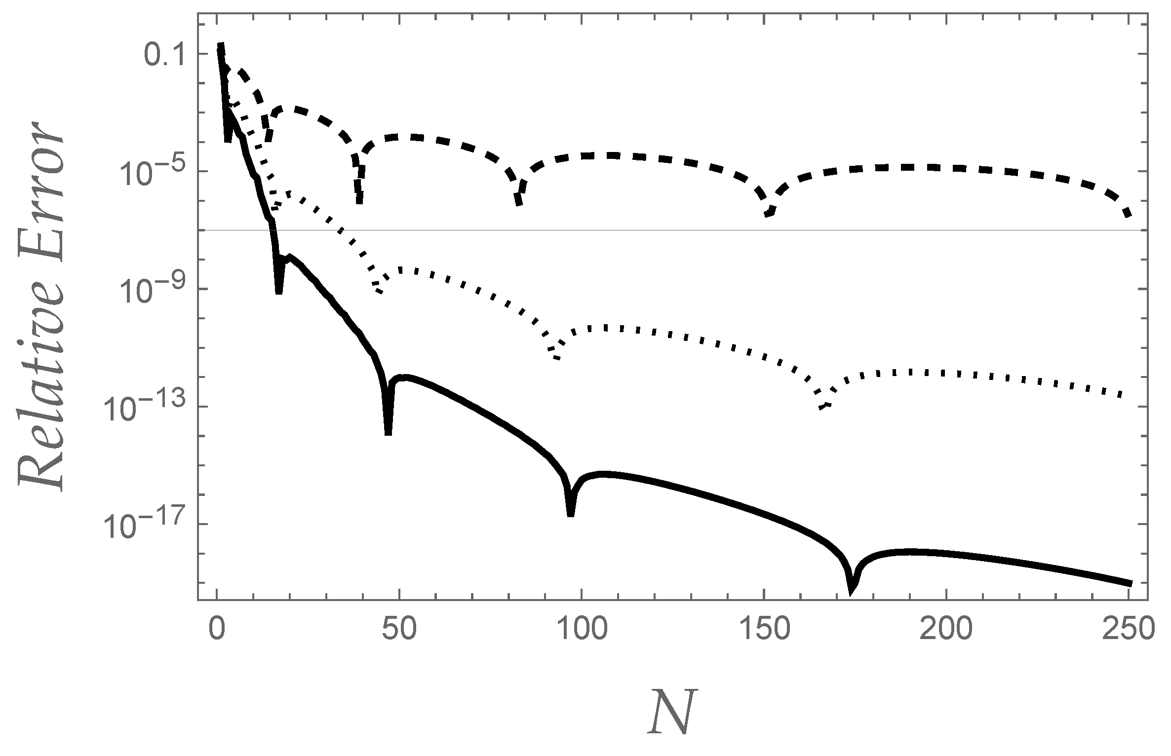
Figure 2.
The same as in Figure 1, but as far as the Stieltjes integral is concerned.
Figure 2.
The same as in Figure 1, but as far as the Stieltjes integral is concerned.
Disclaimer/Publisher’s Note: The statements, opinions and data contained in all publications are solely those of the individual author(s) and contributor(s) and not of MDPI and/or the editor(s). MDPI and/or the editor(s) disclaim responsibility for any injury to people or property resulting from any ideas, methods, instructions or products referred to in the content. |
© 2025 by the authors. Licensee MDPI, Basel, Switzerland. This article is an open access article distributed under the terms and conditions of the Creative Commons Attribution (CC BY) license (http://creativecommons.org/licenses/by/4.0/).
Copyright: This open access article is published under a Creative Commons CC BY 4.0 license, which permit the free download, distribution, and reuse, provided that the author and preprint are cited in any reuse.


