Submitted:
28 July 2025
Posted:
29 July 2025
You are already at the latest version
Abstract
Genetic improvement in wheat yield is the most focused research area for the breeding community to ensure food security and sustainable production. Wheat kernel traits and biomass are considered key contributors to enhance crop yield. A set of 264 doubled haploid (DH) lines mainly derived from two popular Texas wheat cultivars, TAM 114 and TAM 204, were developed at the AgriLife Research Center in Amarillo. The other parents are widely adopted and improved cultivars from the Southern Great Plains. Lines were evaluated in two field environments (Bushland-irrigated & Bush-land-dryland) planted in alpha lattice design during the 2020 crop season. Kernel traits (seed length, width, area, perimeter, and 1000 kernel weight) were collected using the hp Scanjet G4010 photo scanner for image capturing and GrainScan software for image analysis. This procedure offered a high throughput, precise, robust, and cost-effective seed phenotyping platform. Biomass parameters (plant weight, head count, head weight) were collected and processed manually. For genotyping genomic libraries were prepared and sequenced on Illumina NovaSeq 6000 to generate paired end reads of 150 bp. For single nucleotide polymorphism (SNP) calling, sequences were aligned to the IWGSC RefSeq genome assembly v2.1 using the Burrows Wheeler Aligner. The SNP filtration was performed at 50% missing data and 5% minor allele frequency. Finally, a set of 59842 polymorphic markers were retained for genetic analysis. To investigate the marker-trait association and the genomic regions, four genome-wide-association study (GWAS) models were implemented using the R package ‘Genome Association and Prediction Integrated Tool’ (GAPIT). Based on the Bonferroni correction < 8.41E-07 was used as a threshold to declare maker trait associations (MTA) significant. The BLINK model identified 12 MTA on chromosomes 1A, 2A, 2B, 4A, 4B, and 6B. 45% of the lines carried S2A_251496962 marker for the seed perimeter, while 42% and 39% lines carried S2A_498737202 and S2B_792756832 makers for 1000 KW and seed width, respectively. The identified MTA might be representing some known/major genes which need fur-ther confirmation.
Keywords:
association mapping
; kernel traits
; biomass
; winter wheat
; doubled haploids
; image analysis
; Illumina NovaSeq
1. Introduction
The bread wheat (Triticum aestivum L.) feeds almost 30% of the world population and is a major source of up to 25% daily calories consumed by humans globally [1]. Rapid population growth, climate changes and frequent global events of biotic and abiotic stress are big agricultural challenges for sustainable production. The wheat yield needs to be increased 2.5% annually and under current circumstances it is projected that by 2050 overall wheat production should increase up to 70% to meet the future demand [2]. The kernel traits and biomass are very critical elements contributing directly to yield and yield components in wheat and have great potential in exploiting the genetic diversity within the adopted cultivars, conventional germplasm and Triticeae gene pool [3]. Measurement of kernel characteristics is a vital aspect in cereal breeding and genetics and high phenotypic accuracies provide more reliable genetic insights. Manual wheat kernel phenotyping is very laborious, time consuming and expensive, while the GrainScan approach is a high throughput, robust and cost-effective phenotyping platform [4].
Traits contributing to the yield and yield components mainly exhibit polygenic inheritance and controlled by several quantitative trait loci (QTL) and genes [5]. Genome wide association studies (GWAS) and linkage mapping have been widely used to elucidate the genetic mechanisms of complex traits [6,7]. Through several studies the effectiveness of GWAS has been proved to identify the marker trait association for agronomic traits [8], disease resistance [9], end-use quality [10] and yield related traits [11]. In wheat, QTL and genes for spikes [12] and kernel traits have been reported on all chromosomes [13,14]. Few major effect genes and QTL, especially TaGS5, TaSus1, TaSus2, and TaGW2, are significantly associated with kernel size, kernel weight, spike, peduncle length, and grain weight [15,16,17]. The major genes Q & C on chromosomes 5A and 2D, controlling the modern wheat spike morphology are also associated with kernel size, shape, grain yield and 1000 kernel weight [18,19].
Although numerous studies have been conducted to investigate genetics controlling kernel traits and biomass in spring and winter wheat germplasms. The popular cultivated winter wheat varieties in the US Southern Great Plains likely harbor unexplored allelic diversity and potentially new QTL contributing to the kernel traits and overall, to the yield. The wheat genetics program at the Texas A&M AgriLife Research in Amarillo, TX developed an association mapping panel involving the most popular cultivated winter wheat cultivars in the region using the doubled haploid (DH) approach. This approach has been successfully used to pyramid favorable alleles from different sources by reducing the breeding cycles, attaining homozygosity in a short period of time and accelerating the genetic gain in wheat.
This study used a winter wheat DH association mapping panel that was phenotyped for kernel and biomass traits using the high throughput seed scanner and genotyped on the NovaSeq 6000 next generation sequencing platform. We performed GWAS with the objectives to identify genomic regions associated with biomass and kernel traits by integrating the cost-effective and efficient seed scanning approach and exploring the underlying genetics.
2. Materials and Methods
2.1. Association Mapping Panel
The association mapping panel comprised of 264 doubled haploid (DH) lines mainly derived from the cultivated winter wheat varieties ‘TAM 114’ and ‘TAM 204’ in Southern Great Plains. TAM 114 is hard red winter wheat which was developed and released by Texas A&M AgriLife Research in 2014. This is an awned, medium-maturing, semi-dwarf wheat with red glumes. It was released primarily for its extra-strong baking properties, excellent mixing tolerance, and good loaf volume. TAM 114 has a significantly higher grain yield as compared to TAM 111 and TAM 112 in the Texas High Plains under both irrigated and dryland environments. It is high in grain volume weight, is resistant to all three rusts (leaf, stripe, and stem) at the time it was released with a moderate resistance to Hessian fly biotypes GP and vH9 [20]. TAM 204 is a high yielding and drought tolerant variety recommended for the Texas Great Plains. It also provides resistance against wheat streak mosaic virus (WSMV), greenbug (GB), Hessian fly (HF), and wheat curl mite (WCM) [21].
2.1.1. Development of Doubled Haploids (DH)
The wheat genetics lab at the AgriLife Research in Amarillo, TX developed the doubled haploids by pollinating the F1 plants with the corn pollen and treating pollinated spikes with 2,4-Dichlorophenoxyacetic acid (2,4-D) synthetic auxin solution (a plant growth hormone) to induce haploid embryo formation. Two weeks after the pollination, embryos were rescued by dissecting seeds, treated with colchicine solution for chromosome doubling, incubated for 16-24 h at 18 °C and then cultured on the Murashige-Skoog (MS) growth media for 7 days in the dark room. After germination plant seedlings were transferred to the growth chamber until two leaf stage and then vernalized at 4 °C for 6-8 weeks. The vernalized seedlings were transplanted into 2.5-inch pots filled with potting mix and transferred into growth room to recover for 1-2 weeks. Later, the plants were shifted to greenhouses until the physiological maturity. Each plant was assigned a unique identification number based on the parentage during the harvest to develop a population for downstream genetic studies.
2.2. Kernel Phenotyping, Biomass and Statistical Analysis
2.2.1. Experimental Layouts
A set of 264 DH lines was planted in two environments; Bushland irrigated and Bushland dryland (35°06′ N, 102°27′ W) in 2020 hereafter designated as BI20 and BD20. Both locations used an alpha-lattice experimental design with a plot size of 3.05 m long and 1.52 m wide for the irrigated experiments, while the plot size in the drylands was 4.57 m by 1.52 m. Both experiments included four check varieties, TAM 114, TAM 115, TAM 204, TAM 205 in the experimental layout.
2.2.2. Kernel Image Capturing
Approximately 7 to 8 g seeds of each DH line from both environments (BI20 and BD20) were randomly taken and scanned using the hp Scanjet G4010 photo scanner (Hp 11956A, Hewlett-Packard, Palo Alto, CA, USA) which is a consumer grade flatbed scanner (Figure 1A) All images were scanned at 300 dots per inch (DPI) with no color adjustment or cropping applied. The DPI measures the density of dots in an image and describes the resolution of a digital display. For wheat scanning, grains were spread onto a glass bottomed tray for ease of collection (Figure 1B). Since the wheat seed was bulked from field trial material, a non-uniform subsample of seed was scattered from a seed packet. To maximize contrast at the border of each seed, either a piece of black cardboard, or a matte black box was upturned over the scanning surface, minimizing reflection and shadow. To allow standardization of color measurements to the CIELAB colorspace, a Munsell ColorChecker Mini card (X-Rite Corp., MI, USA) was scanned under the same settings as the seed and used within GrainScan to generate conversion parameters for the color information measured by the flatbed scanner (Figure 1C,D). We used an equal amount of seed (7 to 8 g) from each line to avoid excessive touching of grains during the scanning process and ensure separate data point generation from each seed. The number of seeds per image ranged from 201 to 483 with a mean value of 318 in the BD20 environment, while it ranged from 167 to 389 with a mean value of 264 in BI20 environment.
2.2.3. Image Analysis and Data Generation
In GrainScan the image analysis used a grayscale image which was derived from the scanned color image by averaging the red and green channels. We utilized preprocessing that simplified the image, the factors which are used in the simplification process are mainly interconnected components [22]. This preprocessing involves the Gaussian smoothing to reduce noise, based on an attribute on width (0.3 × Min grain width) to fill in the grain crease, a thinning attribute based on elongation to remove background scratches, and attributes based on width (0.7 × Min grain width) and length (0.7 × Min grain length) to remove thin and thick debris, respectively. The Gaussian smoothing or Gaussian blur calculates the average of neighboring values to effectively blur or smooth an image which are based on the computer algorithms. The following formula is used for a 2D Gaussian function to process an image:
where,
G (x, y) = (1/(2 * π * σ^2)) * e^ (-(x^2 + y^2)/(2 * σ^2))
G (x, y): Gaussian value at (x, y) coordinates.
σ (sigma): Standard deviation, controlling the width or blurriness of the Gaussian.
x and y: Horizontal and vertical distances from the center of the Gaussian kernel.
e: Base of the natural logarithm.
π: Mathematical constant (Pi).
The (1/(2 * π * σ^2)) term is a normalization factor that ensures the integral of the Gaussian function over all space is equal to 1. This is important for maintaining the overall brightness of the image.
The grains can be separated from the background through a simple global threshold which is determined by using an automated method. The method is based on a bivariate histogram of input grey level versus gradient. This is a very reliable procedure and commonly used in image normalization [23]. Touching grains are separated using a common binary object splitting technique based on finding the troughs between regional maxima in the smoothed distance transform. To remove any small regions created by the grain splitting step, a filtering based on the connected component area (0.5 × Min grain width × Min grain length) is performed. Individual grains are labelled and measured based on their size and color. The dimensional measurements are area, perimeter, length and width with the major and minor axes of the best fit ellipse (called majellipse and minellipse, respectively). These surrogates are quick to compute and tend to be more robust to noise (small bumps and dents) in the segmented grain boundary which can cause problems with algorithms that measure the exact length and width. The dimension units are converted from pixels to millimetres (mm) based on the input scanner resolution in DPI.
The GrainScan software has two independent procedures while performing the color analysis. The first procedure is to get the color measurements for each grain as CIELAB values rather than the raw RGB values calculated by the scanner. To use the color calibration option, the image of a calibrated color checker card must first be analyzed using ColourCalibration software. This software locates the card, segments each of the color swatches, extracts the mean RGB values for each swatch, and determines the transformation matrix, RGB2Lab, by linear regression between the measured RGB values and the supplied CIELAB values for each swatch. For convenience, the transformation matrix is saved as two images, one containing the 3×3 matrix and one the 3×1 offset. Using the transformation matrix within GrainScan software, the colored measurements made within each labelled grain can be converted from raw RGB values to calibrated L*, a*, and b* values. CIELAB expresses color as three values: L* for perceptual lightness and a* and b* for the four unique colors of human vision; red, green, blue, and yellow.
The GrainScan software version 1.0 [24] calculated the kernel area (Area, mm−2), kernel perimeter (Peri, mm), kernel length (Length, mm), and kernel width (Width, mm) for each individual seed from each DH line. We developed the R script to compile those varying individual data points to get an average trait value for each line. The average trait value was used for genetic analysis. Based on the weight of the scanned seed (e.g., 7g) and numbers of seeds (e.g., 312 seeds) from each DH line we calculate the seed weight kernel−1 (7/312=0.022 g) and 1000 kernel weight (0.022×1000 = 22g).
2.2.4. Biomass Traits
The following above ground biomass traits were recorded on all DH lines in both environments.
- Plant weight (P. Wt, g): A half meter long single row representing the plot was harvested from the 2nd or 3rd row of the plot at the time of physiological maturity, and the wight was measured including the stem, leaves and heads.
- Head count (H. Count): The number of heads were counted and recorded from the same plant
- Head weight (H. Wt, g): Heads were separated from the stems at the base of the spike and all heads were weighed together from the same plant.
2.2.5. Data Analysis
The Pearson correlation coefficients (r) were calculated for all eight traits in both phenotyping environments in ‘R Studio’ using the ‘metan’ package. The basic statistics describing data quality for both data sets were performed in IBM SPSS1.0.0.1174 (IBM Corp.).
2.3. Genotyping and SNP Calling
The 264 DH lines were planted in a 126-well plastic tray filled with cotton balls soaked with distilled water. Trays were placed in the dark room for 48 h for seed germination and later shifted to the growth chamber at 18 °C for a 12 h day length. When plants were grown to two leaf stage approximately 2 cm leaf tissue was harvested in microtubes and lyophilized for 3 days. Plant TissueLyzer II (QIAGEN) was used for grinding leaf tissue, and a BioSprint 96 DNA plant kit was used to extract the DNA on a BioSprint workstation (QIAGEN) [25]. Genomic libraries were prepared using the TrueSeq DNA PCR-Free kit. This kit is specifically designed for the whole-genome sequencing and better coverage for complex genomes. Libraries were denatured and diluted and sequenced on NovaSeq 6000. Demultiplexing was performed using the bioinformatics pipeline to sort reads and separate them by their unique barcodes [26]. For SNP calling, the sequences from were aligned with the IWGSC Chinese Spring wheat genome assembly v2.0. The sequences were aligned with the reference genome using the ALN function in Burrows-Wheeler Aligner using default parameters [27]. Samtools was used to further process the aligned sequences, and the “mpileup” procedure along with bcftools was used for SNP calling [28]. Finally, SNP filtration was performed at 50% missing data and 5% minor allele frequency [29].
2.4. Association Mapping Analysis
To identify the marker-trait associations and the genomic regions, a genome-wide-association study (GWAS) analysis was conducted using the R package ‘Genome Association and Prediction Integrated Tool’ (GAPIT). We implemented four different models called Mixed Linear Model (MLM), Multiple Locus Mixed Linear Model (MLMM), Fixed and random model Circulating Probability Unification (FarmCPU), and Bayesian-information and Linkage-disequilibrium Iteratively Nested Keyway (BLINK). Each model has its own advantages and disadvantages but simply the MLM model can be described using Henderson’s matrix notation as follows:
where Y is the vector of observed phenotypes; β is an unknown vector containing fixed effects, including the genetic marker, population structure (Q), and the intercept; u is an unknown vector of random additive genetic effects from multiple background QTL for individuals/lines; X and Z are the known design matrices; and e is the unobserved vector of residuals. The u and e vectors are assumed to be normally distributed with a null mean and a variance of:
where G = σ2a K with σ2a as the additive genetic variance and K as the kinship matrix. Homogeneous variance is assumed for the residual effect, i.e., R= σ2 eI, where σ2e is the residual variance. The proportion of the total variance explained by the genetic variance is defined as heritability (h2).
In GAPIT, the covariate variables include the first three principal components derived from all the markers and the origin-group. Principal component analysis was performed using all available SNPs. The first principal components were fitted as covariate variables to reduce the false positives due to population stratification. The portion of variance explained by each component was as follows:
where, the total variance was sum of all the eigenvalues of the available SNP data set.
Y = Xβ + Zu + e
In the MLM model, DH lines were considered as a random effect and the relevance among them was derived by a kinship matrix. The elements in the matrix were utilized as similarities and the resultant clusters were visualized using an Unweighted Pair Group Method with Arithmetic Mean (UPGMA) based heatmap in GAPIT package. We used the Bonferroni correction to declare significant marker trait association. This method adjusts the significance level (alpha) to control the family-wise error rate (FWER), which is the probability of making at least one false positive call in the entire analysis. The adjusted significance level () was calculated as follows:
where, alpha is 0.05 and n is the number of tested markers.
The Manhattan plots were derived to observe the association between genotypes and phenotypes, single nucleotide polymorphism (SNPs) were ordered according to their base-pair positions and chromosomes. In the Manhattan plot, the y-axis represented the negative logarithm of p-value derived from the F-test and the x-axis represented the SNP genomic position.
4. Results
4.1. Phenotyping and Statistical Analysis
The seed scanning process resulted in an average of 483 and 264 data points from each DH line in BD20 and BI20 phenotyping environments, respectively. These results were expected from both experiments because in BD20 environment 7-8 g seeds counted a higher number due to stressed growing conditions producing weak seeds, while the BI20 environment has optimal growing conditions with healthy seeds and 7-8 g counted a smaller number of seeds. The phenotypic data for all traits in both environments had continuous distribution spectrum in the DH association mapping panel (Tables S1 and S2). The basic statistical measures for all the eight traits in both phenotyping environment reflected the data quality and phenotyping accuracies. The standard deviations which quantify the spread of individual data points around the sample means were low. The standard errors measured the precision of the sample means as an estimation of the population mean which ranged from 0.0 to 1.4 and 0.0 to 1.3 in BI20 and BD20 environments, respectively (Tables S3 and S4).
Pearson coefficient correlations (r) were highly significant for Length, 1000 KW, Area and Width (r = 0.65 to 0.97) at p < 0.001, while non-significant for P. Wt and H.Wt with Kernal traits in BI20 environment. The H. Count trait was negatively significantly correlated with all the kernel traits (r = -0.32 to -0.43, p <0.001) (Figure 2A). For the BD20 environment, almost similar correlation trends were observed for the kernel traits which had highly positive significant correlation (r = 0.58 to 0.97) at p < 0.001. The biomass traits, H.Count were negatively correlated with kernel traits including kernel weight (r = -0.30 to -0.36) at p < 0.001. In both BD20 and BI20, P.Wt and H.Count were highly correlated (r = 0.51 to 0.58, p < 0.001) but P.Wt was not significantly correlated with all kernel traits (Figure 2A,B).
4.2. Genomic Libraries and SNP Calling
The genomic libraries sequenced on NovaSeq 6000 to generate 150 bp double-ended reads with an average 1.3-1.6 billion reads per sample. Genomic libraries passed the pre- and post-size selection quality control analysis for both size and mass (Agilent size = 50-650 bp; pooled sample concentration = 7 to 11 nM). Approximately 95% of the reads generated passed the Q30 quality criteria with a mean read quality score of 36. The SNP calling pipelined identified 59482 polymorphic markers (Table S5) with up to 50% missing data and 5% minor allele frequency (MAF) before imputation. The total physical distance/length of the genome was 14073.32 Mb with an average 0.236 Mb whole genome marker density. The B genome had a maximum number of polymorphic SNP markers (26366) followed by A genome (22710) and D genome (10406). Chromosome 3B had the highest number of markers (8322), while chromosome 4D had the least number of markers (1079) (Table 1).
4.3. Population Structure, Maker Heterozygosity and Kinship Matrix
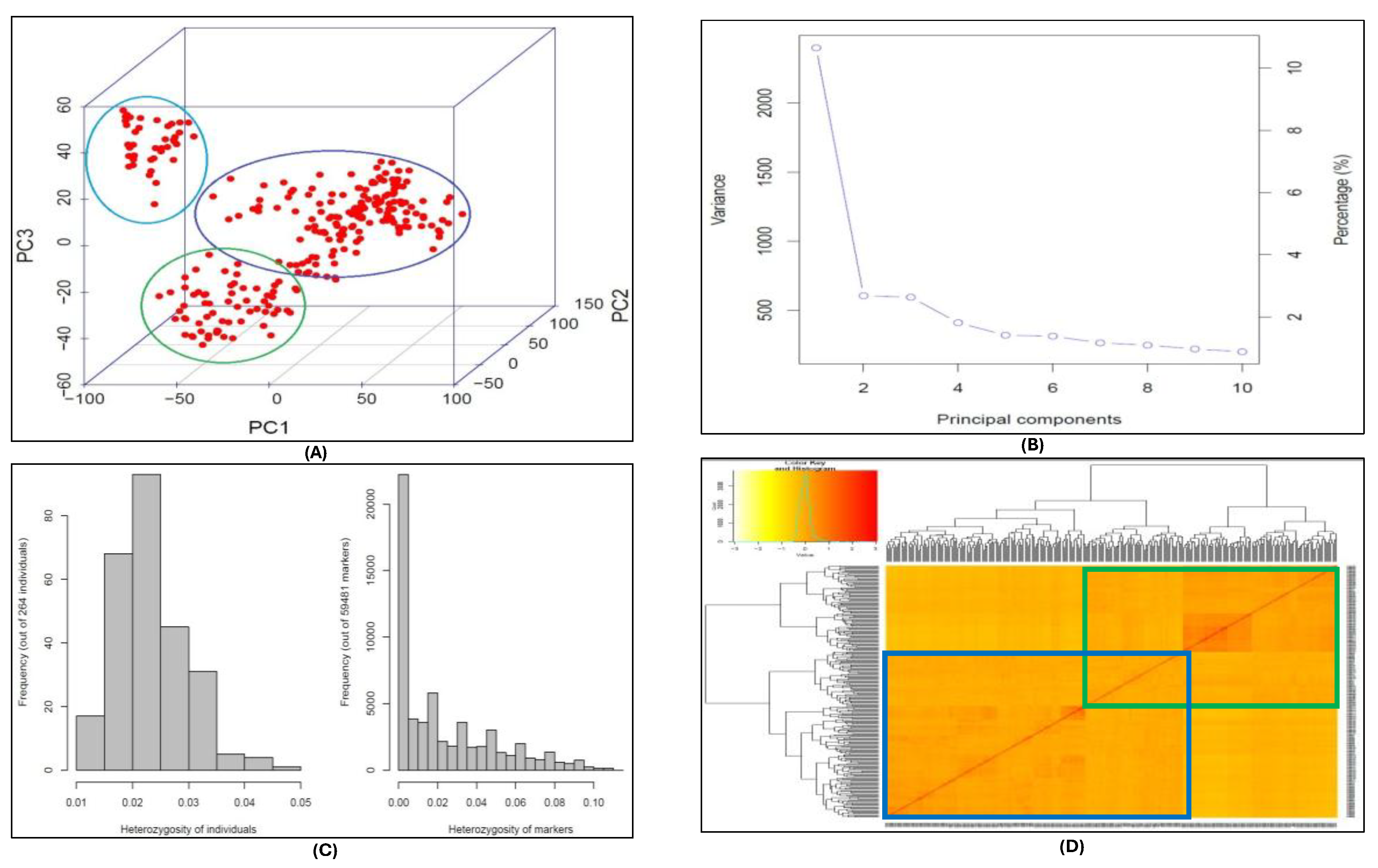
The principal component analysis (PCA) captured the most significant genetic variation within the association mapping panel. The data visualization identified three distinct cluster representing the sub-populations (Figure 4A). The PCA in conjugation with EIGENSTRAT accounted for the population stratification and eigenvectors associated with each PCA showed that the maximum percentage of variation was explained by PC1 followed by PC2, and PC3 accounted for the least variation in the population. The PCA calculated covariance matrix of the data to output its eigenvalues and eigenvectors. Each eigenvalue was associated with an eigenvector also called component vector (Figure 4B). The total variance was 2.05, based on the sum of all the eigenvalues in the SNP data. Among the principal components (PC1, PC2, PC3) the eigenvalues were λ1= 0.80, λ2 = 0.64, and λ3 = 0.60 for each component, respectively. The PC1, PC2, and PC3 explained 39%, 31%, and 29% variation, respectively. (Table S6).
We observed very low heterozygous frequency for both the SNP makers and the DH lines in the population (Figure 4C). The kinship matrix represented the relatedness among individuals with the population and dendrograms depicted clustering of sub-populations within the panel. The dark regions in the heat map show higher co-efficient co-ancestry between individual genotypes and three sub-populations clearly distinguished in the kinship matrix (Figure 4D). Through a closer look at the kinship matrix and the DH line’s pedigree list we were able to distinguish between two large rectangles. The upper right rectangle (Figure 4D; green bordered) in the heat map represents the TAM 204 derived lines, while the lower left rectangle (Figure 4D; blue bordered) represented the TAM 114 derived lines. Furthermore, we also observed subgroups within these two major groups which represented some other lines from the Southern Great Plains that have either TAM 114 or TAM 204 blood in their background. The blue and green rectangles overlap each other in the middle of the heatmap, those lines shared the pedigree from both TAM 114 and TAM 204 varieties.
4.4. Genome wide Association Mapping
For this manuscript, the presented GWAS results are based on the BLINK model due to its computing efficiency and statistical power. The GWAS analysis in GAPIT using the BLINK model identified 12 marker trait associations (MTA) on chromosomes 1A, 2A, 2B, 4A, 4B, and 6B (Table 2). The threshold level to declare a significant MTA was based on the Bonferroni correction. We calculated the adjusted alpha based on the significant p-value =0.05 and 59481 SNP markers which resulted in a p < 8.41E-07 to declare any MTA significant. The LOD values for each significant MTA were based on the -base10 log of the actual p-value. Based on the minor allele frequency (MAF) 45% of the lines carried S2A_251496962 marker for the seed perimeter, while 42% and 39% lines carried S2A_498737202 and S2B_792756832 makers for 1000 KW and seed width, respectively.
5. Discussion
Grain yield in wheat is a highly desirable trait which is mainly polygenic with quantitative inheritance and influenced by the genetic background and environmental factors [30]. There are two essential components, 1000 KW and number of grains m−2 contributing directly to the grain yield. These components have significantly impacted the yield in the wheat breeding history [31]. In the current study we focused on kernel traits including Length, Width, Area, Peri which determine the 1000 KW. This agronomic trait is very stable, and breeders make selection based on 1000 KW during the variety development process [32]. It is evident from previous studies that 1000 KW and other kernel traits have higher contribution to the grain yield as compared to number of grains per spike [33]. This study utilized a set of 264 DH lines developed by the Texas A&M AgriLife Research Wheat Genetics Program and were mainly derived from the popular cultivated wheat varieties form the Southern Great Plains.
The phenotyping data from both environments reflected significant variation for all 8 traits and data distribution was continuous which indicates that traits have polygenic and quantitative inheritance. Measured traits had lower standard deviation which illustrates that data points were clustered closer to trait means values in both environments. Similarly, standard error values for all traits were very small, indicating that the sample means were an accurate representation of the population mean. The kernel traits were highly correlated in both environments, especially Length, Width, Area, and Peri with the 1000 KW which supported the concept that kernel traits contribute to 1000 KW and overall, to the grain yield. Some previous studies have also moderate to higher correlations among 1000 KW and kernel size [34]. It has also been reported that Kernel length and width in both durum and bread wheat positively influence the 1000 KW [35]. We observed a consistent non-significant and negative correlation among biomass and kernel traits in both environments. These negative associations could be explained by the environmental factors contributing to plant growth and seed development (Figure 2A,B).
The illumina NovaSeq 6000 generated on average 1.3-1.6 billion reads per sample with more that 95% reads passed the quality criteria. All 21 chromosomes had good coverage and high marker density. The D genome had overall low marker density which is very common in wheat due to less historical recombination events (Figure 3). A total of 59481 SNP markers were deployed to analyze the population structure and the relatedness among 264 DH lines. The PCA analysis distinguished three sub-populations in the mapping panel. Based on the mathematical calculations of total variance and the phenotypic variance explained by each principal component we were able to verify the genetic variation contributed mainly by three subgroups (Table S6). The frequencies of heterozygous markers and DH lines were low and such results were expected because heterozygous SNP calls were purged during the SNP filtration process and DH lines should have also attained homozygosity during the chromosome doubling process in DH development.
Several GWAS models have been implemented to explore the significant MTA. We used four models using the GAPIT package in R, but the data presented in this manuscript was derived from the BLINK model based on its stringency and low false discovery rate. Moreover, we adopted quite stringent criteria to declare a significant MTA based on the Bonferroni correction. All MTA were considered significant if the corrected p-value was less than 8.41E-07. Several other factors like population, array type, and marker data can influence the threshold level.
In this study, we identified 12 significant MTA on 6 chromosomes (1A, 2A, 2B, 4A, 4B, and 6B). Chromosome 1A had only one MTA where a SNP (S1A_47840044) at 47.84 Mb region was associated with Length. The chromosome 2A had 3 significant MTA for 1000 KW (498.73 Mb), Length (211.35 Mb), and Peri (251.49 Mb) explaining 5.2 to 8.2% phenotypic variance. Chromosome 2B had 4 significant MTA for the Length (664.43 Mb), Peri (702.38 Mb), H. Wt (740.97 Mb), and Width (792.75 Mb) which accounted for 4.4 to 37.1% variation. Chromosomes 4A and 6B each had one significant MTA for 1000 KW (663.09 & 567.70 Mb). Chromosome 4B harbored two significant MTA for Area and Width at 592.4 Mb. Both these traits were associated with the same SNP marker (S4B_592421708) and accounted for 11.7 to 21.6% variation (Table 2). The identified MTA in DH mapping population is contributing considerably higher variation especially for the kernel traits and 1000 KW and could be a great resource for genetic variability and further utilization in the wheat breeding pipeline to develop high yielding cultivars. The identified MTA might represent known major genes and QTL previously identified in the same genomic regions which need further insights to verify their novelty.
Figure 4.
Population structure analysis of DH wheat association mapping panel. (A) Principal component analysis (PCA) showing three sub-populations in the mapping panel. (B) The percentage of the variance explained by the principal components. (C) Frequency of heterozygous DH lines in the association mapping panel and heterozygous markers. (D) Heat map of kinship matrix representing relatedness among the population. The darker regions show higher co-efficient co-ancestry between genotypes and dendrograms depicts clustering of sub-populations within the panel.
Supplementary Materials
The following supporting information can be downloaded at the website of this paper posted on Preprints.org, Table S1: Phenotypic data of association mapping panel from Bushland irrigated (BI) environment in 2020. Table S2: Phenotypic data of association mapping panel from Bushland dryland (BD) environment in 2020. Table S3: Basic statistics on all eight phenotypic parameters for data quality in Bushland irrigated (BI) environment in 2020. Table S4: Basic statistics on all eight phenotypic parameters for data quality in Bushland dryland (BD) environment in 2020. Table S5: Genotypic data on 264 doubled haploid lines using NovaSeq 6000. Table S6: Variance explained by each principal component.
Author Contributions
YR.; Performed formal data analysis and prepared the original manuscript draft, ZW.; Collected seed images and assisted image analysis script writing for data compilation, KP.; Performed bioinformatics pipeline for SNP calling and genetics data filtration, SB & JB.; conducted field trials in both Bushland irrigated and Bushland dryland environments, JR, XQ, AI.; provided experimental and project administration resources, SL.; Conceptualization, funding acquisition, supervision and resources. All authors have read and agreed to the published version of the manuscript.
Funding
This research received no external funding.
Institutional Review Board Statement
This study did not require ethical approval.
Data Availability Statement
All the data attached as “Supplementary Data” will be publicly available.
Conflicts of Interest
The authors declare that the research was conducted in the absence of any commercial or financial relationships that could be construed as a potential conflict of interest.
Abbreviations
The following abbreviations are used in this manuscript:
| SNP | Single Nucleotide Polymorphism |
| MAF | Minor Allele Frequency |
| PVE | Phenotypic Variance Explained |
| LD | Linkage Disequilibrium |
| QTL | Quantitative Trail Loci |
| GWAS | Genome Wide Association Study |
| DH | Doubled Haploid |
| GAPIT | Genome Association and Prediction Integrated Tool |
| MLM | Mixed Linear Model |
| MLMM | Multiple Locus Mixed Linear Model |
| BLINK | and Bayesian-information and Linkage-disequilibrium Iteratively Nested Keyway |
| FarmCPU | Fixed and random model Circulating Probability Unification |
| DPI | Dots Per Inch |
| BD | Bushland Dryland |
| BI | Bushland Irrigated |
| MTA | Marker Trait Association |
| PCA | Principal Component Analysis |
| UPGMA | Unweighted Pair Group Method with Arithmetic Mean |
References
- Rabieyan, E.; Alipour, H. NGS-based multiplex assay of trait-linked molecular markers revealed the genetic diversity of Iranian bread wheat landraces and cultivars. Crop Pasture Sci. 2021, 72, 173–182. [Google Scholar] [CrossRef]
- Li, P. et al. Wheat breeding highlights drought tolerance while ignores the advantages of drought avoidance: A meta-analysis. Eur. J. Agron. 2021, 122, 126196. [CrossRef]
- Mujeeb-Kazi, A.; Gul, A.; Ahmad, I.; Farooq, M.; Rauf, Y.; -ur Rahman, A.; Riaz, H. Genetic resources for some wheat abiotic stress tolerances. In Salinity and Water Stress: Improving Crop Efficiency, 2009, pp. 149-163. Dordrecht: Springer Netherlands.
- Ramya, P.; Chaubal, A.; Kulkarni, K.; Gupta, L.; Kadoo, N.; Dhaliwal, H.S.; Chhuneja. P.; Lagu, M.; Gupt, V. QTL mapping of 1000-kernel weight, kernel length, and kernel width in bread wheat (Triticum aestivum L.). J. Appl. Genet. 2010, 51:421–429. [CrossRef]
- Fan, M., Zhang, X., Nagarajan, R., Zhai, W., Rauf, Y., Jia, H., Yan, L. Natural variants and editing events provide insights into routes for spike architecture modification in common wheat. The Crop J. 2023, 11(1), 148-156. [CrossRef]
- Zhang, D.; Fan, M.; Li, T.; Rauf, Y.; Liu, Y.; Zhu, X.; Jia, H.; Zhai, W.; Luzuriaga, J. C.; Carver, B. F.; Yan, L. A natural allele of the transcription factor gene TaMYB-D7b is a genetic signature for phosphorus deficiency in wheat. Plant Physiology, 2025, kiaf224. [CrossRef]
- Wu, J.Z.; Qiao, L.Y.; Liu, Y.; Fu, B.S.; Ragupathi, N.; Rauf, Y.; Jia, H.Y.; Yan, L. Rapid identification and deployment of major genes for flowering time and awn traits in common wheat. Front. Plant Sci. 13 (2022) 992811. [CrossRef]
- Sun, C.; Zhang, F.; Yan, X.; Zhang, X.; Dong, Z.; Cui, D.; Chen, F. Genome-wide association study for 13 agronomic traits reveals distribution of superior alleles in bread wheat from the Yellow and Huai Valley of China. Plant Biotech J. 2017, 15, 953–969. [Google Scholar] [CrossRef] [PubMed]
- Zhang, J.; Gill, H.S.; Halder, J.; Brar, N.K.; Ali, S.; Bernardo, A.; Amand, P.S.; Bai, G.; Turnipseed, B.; Sehgal, S.K. Multi-locus genome-wide association studies to characterize Fusarium head blight (FHB) resistance in hard winter wheat. Frontiers in Plant Sci. 2022, 13, 946700. [Google Scholar] [CrossRef] [PubMed]
- Chen, J.; Zhang, F.; Zhao, C.; Lv, G.; Sun, C.; Pan, Y.; Guo, X.; Chen, F. Genome-wide association study of six quality traits reveals the association of the TaRPP13L1 gene with flour colour in Chinese bread wheat. Plant Biotech. J. 2019, 17, 2106–2122. [Google Scholar] [CrossRef] [PubMed]
- Singh, K.; Saini, D.K.; Saripalli, G.; Batra, R.; Gautam, T.; Singh, R. WheatQTLdb V2.0: A supplement to the database for wheat QTL. Mol. Breeding 2022, 42, 56. [Google Scholar] [CrossRef] [PubMed]
- Gao, F.; Wen, W.; Liu, J.; Rasheed, A.; Yin, G.; Xia, X.; Wu, X.; He, Z. Genome-wide linkage mapping of QTL for yield components, plant height and yield-related physiological traits in the Chinese wheat cross Zhou 8425B/Chinese Spring. Front. in Plant Sci. 2015, 6, 1099. [Google Scholar] [CrossRef] [PubMed]
- Chen, G.; Zhang, H.; Deng, Z.; Wu, R.; Li, D.; Wang, M.; Tian, J. Genome-wide association study for kernel weight-related traits using SNPs in a Chinese winter wheat population. Euphytica 2016, 212, 173–185. [Google Scholar] [CrossRef]
- Jaiswal, V.; Gahlaut, V.; Mathur, S.; Agarwal, P.; Khandelwal, M.K.; Khurana, J.P.; Tyagi, A.K.; Balyan, H.S.; Gupta, P.K. Identification of novel SNP in promoter sequence of TaGW2-6A associated with grain weight and other agronomic traits in wheat (Triticum aestivum L.). PLoS ONE 2015, 10, e0129400. [Google Scholar] [CrossRef] [PubMed]
- Bednarek, J.; Boulaflous, A.; Girousse, C.; Ravel, C.; Tassy, C.; Barret, P.; Bouzidi, M.F.; Mouzeyar, S. Down-regulation of the TaGW2 gene by RNA interference results in decreased grain size and weight in wheat. J. of Exp. Botany 2012, 63, 5945–5955. [Google Scholar] [CrossRef] [PubMed]
- Hou, J.; Jiang, Q.; Hao, C.; Wang, Y.; Zhang, H.; Zhang, X. Global selection on sucrose synthase haplotypes during a century of wheat breeding. Plant Physiology 2014, 164, 1918–1929. [Google Scholar] [CrossRef] [PubMed]
- Ma, L.; Li, T.; Hao, C.; Wang, Y.; Chen, X.; Zhang, X. TaGS5-3A, a grain size gene selected during wheat improvement for larger kernel and yield. Plant Biotech. J. 2016. 14, 1269–1280. [CrossRef] [PubMed]
- Johnson, E.B.; Nalam, V.J.; Zemetra, R.S.; Riera-Lizarazu, O. Mapping the compactum locus in wheat (Triticum aestivum L.) and its relationship to other spike morphology genes of the Triticeae. Euphytica 2008, 163, 193–201. [Google Scholar] [CrossRef]
- Xie, Q.; Li, N.; Yang, Y.; Lv, Y.; Yao, H.; Wei, R.; Sparkes, D.L.; Ma, Z. Pleiotropic effects of the wheat domestication gene Q on yield and grain morphology. Planta 2018, 247, 1089–1098. [Google Scholar] [CrossRef] [PubMed]
- Rudd, J.C.; Devkota, R.N.; Ibrahim, A.M.; Baker, J.A.; Baker, S.; Sutton, R.; Simoneaux, B.; Opena, G.; Hathcoat, D.; Awika, J.M.; Nelson, L.R.; Liu, S.; Xue, Q.; Bean, B.; Neely, C.B.; Duncan, R.W.; Seabourn, B.W.; Bowden, R.L.; Jin, Y.; Chen, M.; Graybosch, R.A.‘TAM 204’ wheat, adapted to grazing, grain, and graze-out production systems in the southern high plains. J. Plant Reg. 2019, 382: 377–382. [CrossRef]
- Rudd, J.C.; Devkota, R.N.; Ibrahim, A.M.; Baker, J.A.; Baker, S.; Lazar, M.D.; Sutton, R.; Simoneaux, B.; Opena, G.; Rooney, L.W.; Awika, J.M.; Liu, S.; Xue, Q.; Bean, B.; Duncan, R.W.; Seabourn, B.W.; Bowden, R.L.; Jin, Y.; Chen, M.S.; Graybosch, R.A. ‘TAM 114’ wheat, excellent bread-making quality hard red winter wheat cultivar adapted to the southern high plains. J. Plant Reg. 2018, 12 (3): 367. [CrossRef]
- Salembier Clairon P.J.; Wilkinson, M. Connected operators: A review of region-based morphological image processing techniques. IEEE Signal Process. Mag 2009, 26:136–157.
- Sintorn I-M.; Bischof, L.; Jackway, P.; Haggarty, S.; Buckley, M. Gradient based intensity normalization. J. Microsc. 2010, 240:249–258. [CrossRef]
- Whan, A.P., Smith, A.B., Cavanagh, C.R. et al. GrainScan: a low cost, fast method for grain size and colour measurements. Plant Methods 10, 23 (2014). [CrossRef]
- Rauf, Y.; Bajgain, P.; Rouse, M. N.; Khanzada, K. A.; Bhavani, S.; Huerta-Espino, J.; Singh, R. P.; Imtiaz, M.; Anderson, J. A. Molecular characterization of genomic regions for adult plant resistance to stem rust in a spring wheat mapping population. Plant Disease, 2022, 106(2), 439–450. [CrossRef]
- Rauf, Y.; Lan, C.; Randhawa, M.; Singh, R. P.; Huerta-Espino, J.; Anderson, J. A. Quantitative trait loci mapping reveals the complexity of adult plant resistance to leaf rust in spring wheat ‘Copio.’ Crop Science, 2022, 62(3), 1037–1050. [CrossRef]
- Li, H.; Durbin, R. Fast and accurate short read alignment with Burrows–Wheeler transform. Bioinformatics. 2009, 25:1754-1760. [CrossRef]
- Li, H. A statistical framework for SNP calling, mutation discovery, association mapping and population genetical parameter estimation from sequencing data. Bioinformatics. 2011, 27:2987-2993. [CrossRef]
- Wang, Z.; Dhakal, S.; Cerit, M.; Wang, S.; Rauf, Y.; Yu, S.; Maulana, F.; Huang, W.; Anderson, J.D.; Ma, X.F.; et al. QTL mapping of yield components and kernel traits in wheat cultivars TAM 112 and Duster. Front Plant Sci. 2022, 13, 1057701. [Google Scholar] [CrossRef] [PubMed]
- Li, T.; Deng, G.; Su, Y.; Yang, Z.; Tang, Y.; Wang, J. Genetic dissection of quantitative trait loci for grain size and weight by high-resolution genetic mapping in bread wheat (Triticum aestivum L.). Theor. Appl. Genet. 2022, 135, 257–271. [Google Scholar] [CrossRef] [PubMed]
- Kumari, S.; Jaiswal, V.; Mishra, V.K.; Paliwal, R.; Balyan, H.S.; Gupta, P.K. QTL mapping for some grain traits in bread wheat (Triticum aestivum L.). Physiol. Mol. Biol. Plants 2018, 24, 909–920. [Google Scholar] [CrossRef] [PubMed]
- Duan, X.; Yu, H.; Ma, W.; Sun, J.; Zhao, Y.; Yang, R. A major and stable QTL controlling wheat thousand grain weight: identification, characterization, and CAPS marker development. Mol. Breed. 2020, 40, 68. [Google Scholar] [CrossRef]
- Ji, G.; Xu, Z.; Fan, X.; Zhou, Q.; Chen, L.; Yu, Q. Identification and validation of major QTL for grain size and weight in bread wheat (Triticum aestivum L.). Crop J. 2022, 11, 564–572. [Google Scholar] [CrossRef]
- Rasheed, A.; Xia, X.; Ogbonnaya, F.; Mahmood, T.; Zhang, Z.; Kazi., A. M. Genome-wide association for grain morphology in synthetic hexaploid wheats using digital imaging analysis. BMC Plant Biol. 2018, 14. [CrossRef]
- Simmonds, J.; Scott, P.; Brinton, J.; Mestre, T.C.; Bush, M.; Del Blanco, A. A splice acceptor site mutation in TaGW2-A1 increases thousand grain weight in tetraploid and hexaploid wheat through wider and longer grains. Theor. Appl. Genet. 2016, 129, 1099–1112. [Google Scholar] [CrossRef] [PubMed]
Figure 1.
Wheat seed scanning and image processing; a high throughput, robust and cost-effective seed trait phenotyping approach. (A) Scanjet G4010 photo scanner (Hp 11956A, Hewlett-Packard, Palo Alto, CA, USA) with a piece of black cardboard, or a matte black box over the scanning surface to minimize reflection and shadow. (B)Wheat seeds scattered on the flat screen, avoiding seed contacts at pre-image capturing stage. (C) Post-seed scanning output image with color calibration and each colored dot represents a single data point for downstream image analysis. (D) Munsell ColorChecker Mini card used for standardization of color measurements to the CIELAB colorspace.
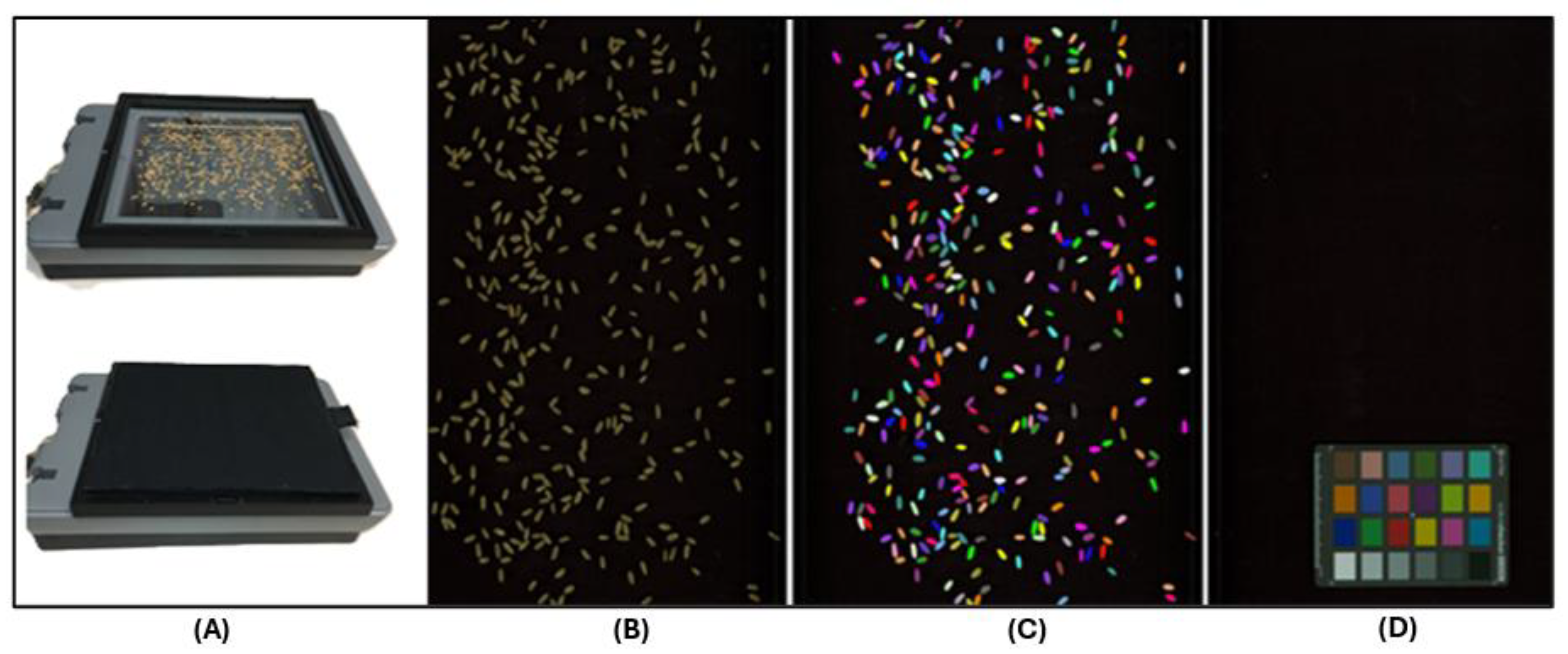
Figure 2.
Pearson correlation coefficient (r) among all traits in both phenotyping environments. (A) BI20 represents Bushland irrigated and (B) BD20 represents Bushland dryland environments in 2020 crop cycle. The correlations with p >= 0.05 are non-significant represented as ‘ns’, while the correlations with p < 0.05, 0.01, and 0.001 are significant and represented by asterisks (*, **, ***), respectively.
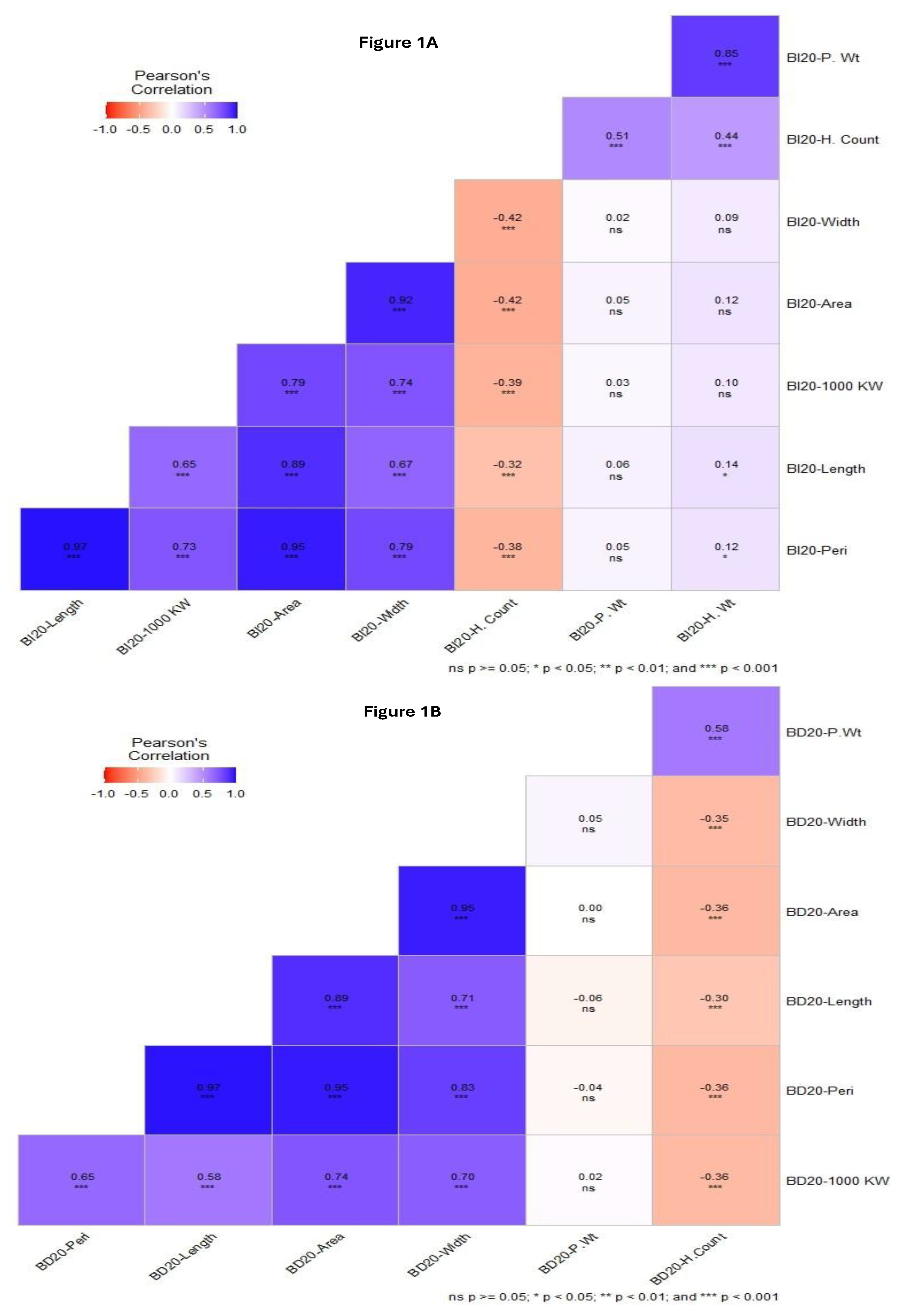
Figure 3.
SNP marker distribution and SNP density across 21 wheat chromosomes. The vertical lines of different colors represent the SNP density within 5 Mb window size.
Figure 3.
SNP marker distribution and SNP density across 21 wheat chromosomes. The vertical lines of different colors represent the SNP density within 5 Mb window size.
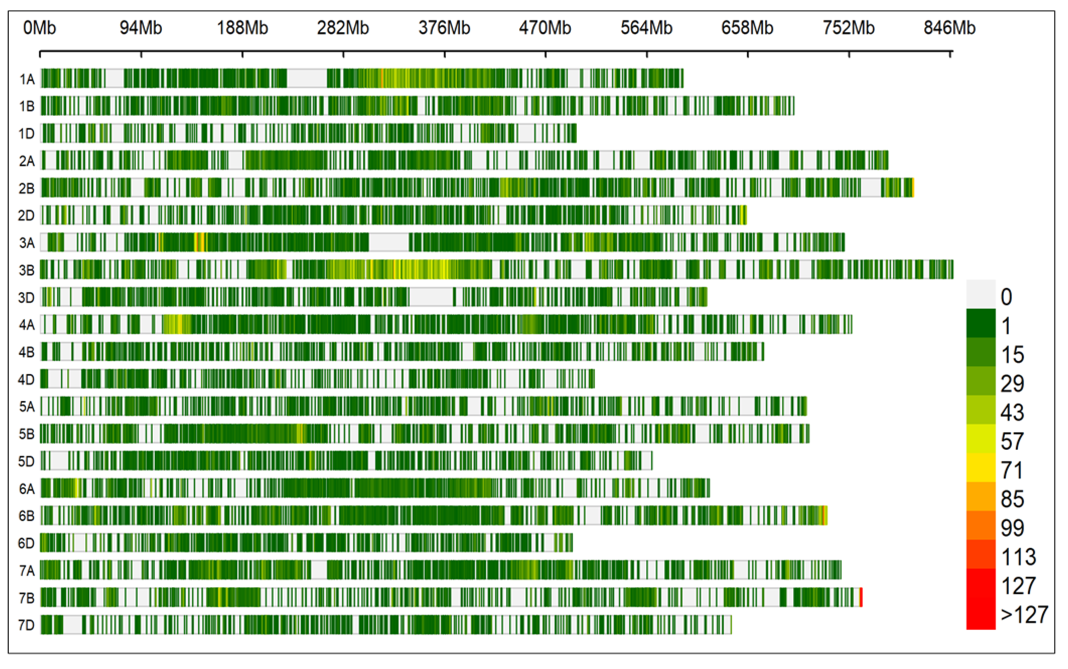

Table 1.
Density and marker distribution across all 21 chromosomes in wheat doubled haploid mapping population.
Table 1.
Density and marker distribution across all 21 chromosomes in wheat doubled haploid mapping population.
| Ch | Start position | End position | Length (Mb) | No. of markers | Marker Density |
|---|---|---|---|---|---|
| 1A | 1.95 | 597.36 | 595.41 | 4465 | 0.133 |
| 1B | 1.42 | 700.37 | 698.95 | 3094 | 0.226 |
| 1D | 2.88 | 498.05 | 495.17 | 1168 | 0.424 |
| 2A | 2.4 | 787.72 | 785.32 | 2858 | 0.275 |
| 2B | 1.88 | 812.03 | 810.15 | 3581 | 0.226 |
| 2D | 2.22 | 565.44 | 563.22 | 2058 | 0.274 |
| 3A | 7.23 | 747.44 | 740.21 | 3912 | 0.189 |
| 3B | 0.07 | 848.26 | 848.19 | 8322 | 0.102 |
| 3D | 2.69 | 619.37 | 616.68 | 1869 | 0.330 |
| 4A | 4.02 | 754.04 | 750.02 | 3451 | 0.217 |
| 4B | 1.74 | 672.25 | 670.51 | 1567 | 0.428 |
| 4D | 0.46 | 514.92 | 514.46 | 1079 | 0.477 |
| 5A | 0.85 | 712.17 | 711.32 | 1902 | 0.374 |
| 5B | 0.08 | 714.55 | 714.47 | 3297 | 0.217 |
| 5D | 1.58 | 568.63 | 567.05 | 1487 | 0.381 |
| 6A | 1.54 | 621.88 | 620.34 | 2765 | 0.224 |
| 6B | 1.31 | 731.18 | 729.87 | 3980 | 0.183 |
| 6D | 0.06 | 494.6 | 494.54 | 1433 | 0.345 |
| 7A | 0.23 | 743.92 | 743.69 | 3357 | 0.222 |
| 7B | 1.04 | 763.61 | 762.57 | 2525 | 0.302 |
| 7D | 1.25 | 642.43 | 641.18 | 1312 | 0.489 |
| Whole genome | 14073.32 | 59482 | 0.236 | ||
Table 2.
Significant marker trait associations identified using the BLINK model for eight traits in two environments.
Table 2.
Significant marker trait associations identified using the BLINK model for eight traits in two environments.
| SNP | Position (bp) | Position (Mb) | Chr | p value | LOD | MAF | PVE | Environment/Trait |
|---|---|---|---|---|---|---|---|---|
| S1A_47840044 | 47840044 | 47.840044 | 1A | 3.09E-08 | 7.51 | 0.05 | 10.6 | BI20. Length |
| S2A_498737202 | 498737202 | 498.737202 | 2A | 7.41E-10 | 9.13 | 0.42 | 08.2 | BD20.1000 KW |
| S2A_211351736 | 211351736 | 211.351736 | 2A | 4.02E-08 | 7.4 | 0.06 | 05.2 | BI20. Length |
| S2A_251496962 | 251496962 | 251.496962 | 2A | 6.49E-08 | 7.19 | 0.45 | 05.7 | BD20. Peri |
| S2B_664436363 | 664436363 | 664.436363 | 2B | 1.86E-10 | 9.73 | 0.09 | 37.1 | BD20. Length |
| S2B_702381983 | 702381983 | 702.381983 | 2B | 1.13E-09 | 8.95 | 0.13 | 04.4 | BD20. Peri |
| S2B_740979562 | 740979562 | 740.979562 | 2B | 2.51E-09 | 8.6 | 0.33 | 13.8 | BI20. H.Wt |
| S2B_792756832 | 792756832 | 792.756832 | 2B | 6.17E-08 | 7.21 | 0.39 | 17.3 | BD20. Width |
| S4A_663097002 | 663097002 | 663.097002 | 4A | 3.96E-11 | 10.4 | 0.23 | 31.8 | BD20.1000 KW |
| S4B_592421708 | 592421708 | 592.421708 | 4B | 1.83E-13 | 12.74 | 0.25 | 11.7 | BD20. Area |
| S4B_592421708 | 592421708 | 592.421708 | 4B | 4.33E-12 | 11.36 | 0.25 | 21.6 | BD20. Width |
| S6B_567706088 | 567706088 | 567.706088 | 6B | 7.69E-09 | 8.11 | 0.25 | 11.2 | BD20.1000 KW |
SNP: Single nucleotide polymorphism. Chr: Chromosome name. p-value: Threshold level to declare a marker trait association significant. Calculated based on the Bonferroni correction. MAF: Minor allele frequency. PVE: Phenotypic variance explained.
Disclaimer/Publisher’s Note: The statements, opinions and data contained in all publications are solely those of the individual author(s) and contributor(s) and not of MDPI and/or the editor(s). MDPI and/or the editor(s) disclaim responsibility for any injury to people or property resulting from any ideas, methods, instructions or products referred to in the content. |
© 2025 by the authors. Licensee MDPI, Basel, Switzerland. This article is an open access article distributed under the terms and conditions of the Creative Commons Attribution (CC BY) license (http://creativecommons.org/licenses/by/4.0/).
Copyright: This open access article is published under a Creative Commons CC BY 4.0 license, which permit the free download, distribution, and reuse, provided that the author and preprint are cited in any reuse.


