Submitted:
28 July 2025
Posted:
29 July 2025
You are already at the latest version
Abstract
In this work, we represent and analyze the Collatz sequences in base-6 system and deduce a finite state machine that describes them. This representation of the sequences sheds the light on an interesting insight such as the existence of only four basic types of cycles which constitute any Collatz trajectory. In turn, this allows us to further treat the Collatz process as a Markov chain and, based on the dataset of the first 107 sequences, computationally show that it has a steady state. Moreover, the steady state probabilities theirselves can be directly used to show that the multiplicative factor of a trajectory for any given starting number is less than 1, that is, on average the trajectories tend to converge.
Keywords:
Collatz conjecture
; Collatz sequences
; base-6 system
; Markov chains
1. Introduction
The Collatz conjecture, also known as the problem, is a deceptively simple mathematical puzzle that has intrigued both amateur and professional mathematicians for decades. It is based on a simple iterative procedure: for any positive integer x apply the rule
This function, known as the Collatz function, generates a sequence by repeatedly applying the rule to its own output. The conjecture posits that no matter what positive integer one starts with, the sequence will eventually reach the number 1, at which point it enters a repeating cycle of .
Despite its elementary formulation, the problem remains unsolved and is widely believed to be extraordinarily difficult. Its iterations display a mixture of regular patterns and apparent randomness, making rigorous analysis challenging. The problem has been reformulated and generalized in numerous ways and has deep connections to fields such as number theory, dynamical systems, ergodic theory, and computation theory. Among these, the use of Markov chains has emerged as a powerful tool to understand the statistical behavior of iterates under the 3x + 1 transformation.
Early work by Terras and Everett motivated the use of probabilistic models by noting that the parity of the iterates—odd or even—could often be treated as approximately random. This observation led to the development of stochastic models, particularly Markov chains, to describe the evolution of the iterates under probabilistic assumptions.
In the influential survey by Lagarias [1], Markov models are presented as a means to approximate the trajectory behavior of iterates, particularly by analyzing the expected stopping time and growth rates of sequences. The model considers transitions based on parity and yields expected values for the number of steps required to reach 1. The state space of the Markov chain is constructed by considering the residues of iterates modulo powers of 2, which aligns with the conditional nature of the Collatz function.
Matthews [2] provides a comprehensive treatment of how generalized 3x+1 mappings can be interpreted through Markov chains and ergodic theory. By analyzing the behavior of trajectories modulo a fixed integer m, Matthews constructs transition matrices that model the frequency with which iterates fall into particular congruence classes. These models allow for predictions about whether trajectories will converge to cycles or diverge based on the growth rate of iterates. Notably, in the relatively prime case—where multipliers in the generalized mapping are coprime to the modulus—the associated Markov chains are well-behaved and lead to concrete conjectures about limiting distributions and trajectory types.
Crandall [3] earlier hinted at a probabilistic structure underlying the 3x+1 problem by proposing a random-walk heuristic, where each iteration step is modeled as a random variable depending on the exponent of 2 dividing the iterate. This yields a net negative expected logarithmic drift, suggesting eventual convergence to 1. Although not framed in terms of Markov chains, Crandall’s approach lays foundational intuition for later stochastic modeling.
Leigh [4] extends this perspective by formulating a Markov process underlying the generalized Syracuse algorithm, providing further formalism to link probabilistic transitions with deterministic rules of the 3x+1 type. His work contributes to the understanding of how probabilistic models can simulate and forecast the long-term behavior of such systems.
Together, these studies demonstrate the utility of Markov chains in providing a statistical lens on the deterministic but chaotic behavior of 3x+1-type functions. While no probabilistic model has yet resolved the original conjecture, they offer frameworks for exploring the frequency distribution, ergodicity, and growth dynamics of iterates in both the classical and generalized cases.
The current work also attempts to approach the problem from the perspective of stochastic Markov chains as well as numerical simulations.
2. Behavior of Collatz Operations in Base-6 System
The main idea of this work is to analyze the numbers of the Collatz sequences in base-6 system where each number is represented using digits 0 to 5. Therefore, the goal of this section is to understand how the Collatz operations modify the subsequent numbers and show the patterns that occur. It should be noted that this is not exactly the analysis in modulo 6 as it will be apparent further.
Without loss of generality, we restrict our domain only to positive odd integers as the starting numbers of the Collatz sequences (or trajectories), because, clearly, any initial even number will undergo several operations reaching its odd divisor. Hence, we are interested in the odd numbers of the form , , and , for some integer , and the first operation that will be performed on them is .
Let us see where the these numbers will be mapped by this operation. At this point it is more convenient to represent a number with as with and .
1.
- 1) (base 6). This means that the operation will map the number to some other number which ends with "04" in base 6 notation (including 4 for ). Below we proceed in a similar manner.
- 2) (base 6).
2.
- 3) (base 6).
- 4) (base 6).
3.
- 5) (base 6).
- 6) (base 6).
Since all the resulting numbers after this stage are even and end with 4, then the next operation will be . It is not difficult to show that the numbers which end with 04, 24, and 44 will be mapped to the numbers that end with 2 (including 2 itself), whereas the numbers that end with 14, 34, and 54 will be mapped to the numbers which end with 5. Thus, there are only two possibilities for the ending – 2 or 5.
Finally, let us see where the latter numbers will be mapped. Obviously, the numbers that end with 5 are odd and they will again follow the patterns outlined in 3. However, some words need to be said about the numbers that end with 2.
Because a numbers that ends with 2 is even, it will undergo the operation. Here, there are two options:
(1) If the preceding digit in base 6 is even, i.e. {...02, ...22, ...42}, then clearly the number after the operation will end with 1, for example, . This again brings us to the 1.
(2) If the preceding digit base 6 is odd, i.e. {...12, ...32, ...52}, then the number after the operation can end only with 4, for example, and . This means we need to perform one more operation which will lead us again to some number that ends with 2 or 5.
By following the procedure as described above and looking at the endings of the resulting numbers in base-6 system, we notice that it is a repetitive process and, thus, can be represented by some finite state machine which will be shown in the next section. It is worth mentioning that this procedure is purely deterministic.
3. Base-6 Finite State Machine
As we have discovered in the previous section, the procedure of generating the Collatz trajectories can be described by some finite state machine (FSM). The diagram of such an FSM can be as depicted in the Figure 1.
The FSM contains 4 states - A, B, C, and D. Each state corresponds to the number from Collatz trajectory depending on the ending in base-6 system as described above. For example, the state A corresponds to the numbers that end with 1 (including 1 as well), 3, and 5. The transitions (arrows) between the states of the FSM correspond to the Collatz operations: green - , red - . The starting state is always the state A. Unless the Collatz conjecture is proven, the FSM will either stop at the state A, if the sequence reaches 1, or loop forever.
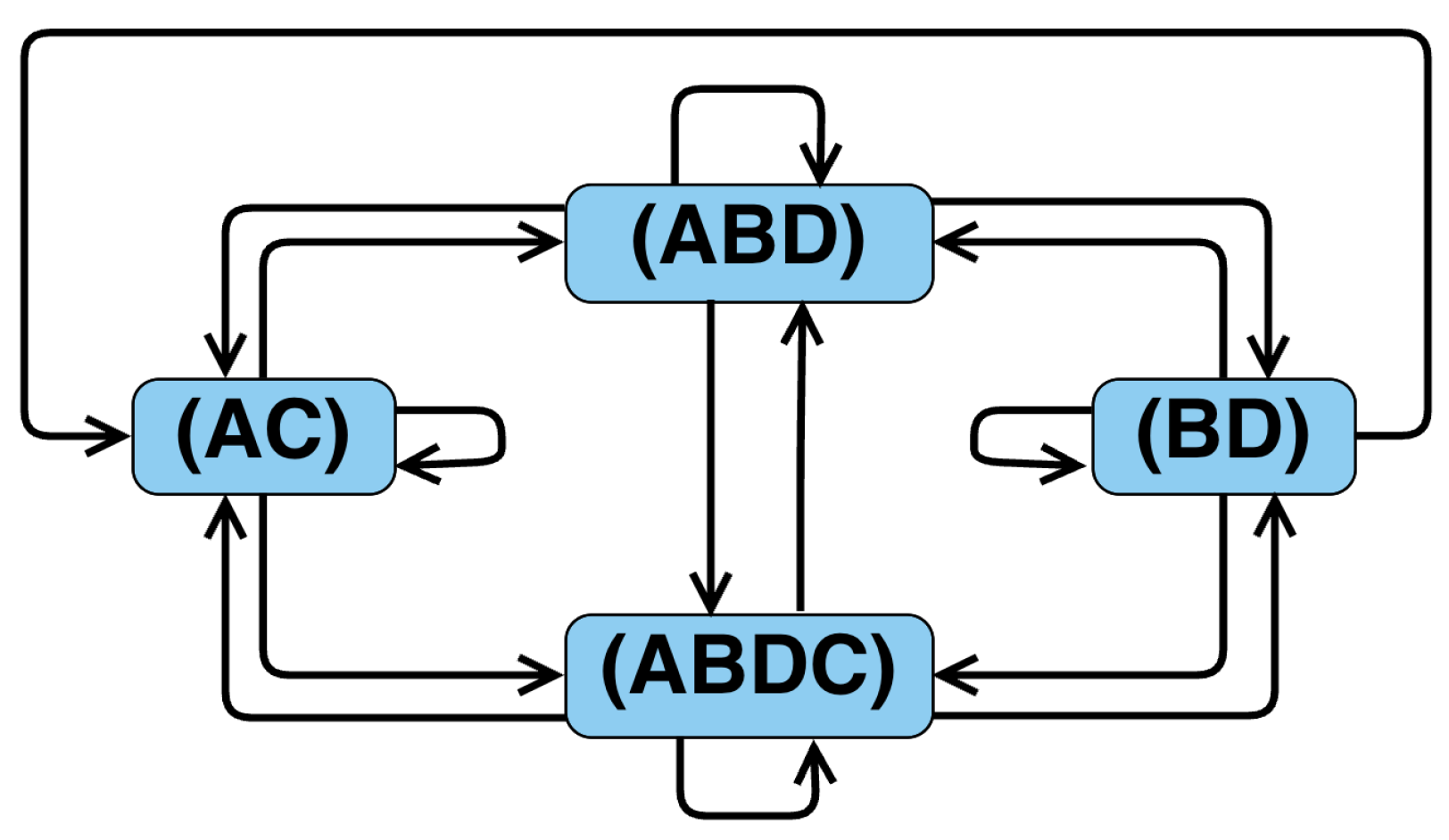
One can notice that some arrows point to the internal (orange) boxes while the others point to the outer (blue) boxes. This is done intentionally just to show where numbers could go specifically. However, we are interested in the outer (blue) boxes which we call states. Therefore, to simplify the analysis we will use the aggregated version of the FSM shown in the Figure 2.
Note also that this is not the only FSM and one could choose another (maybe, more fine-grained) version as long as it obeys the procedure and the patterns outlined in the previous section. Moreover, we could add one more state to the current model to define the final state where the last number (namely, 1) in the Collatz sequences would go, but we don’t want to make such a strong assumption as the existence of the final 1 is been hypothesized. For our purposes, the version in Figure 2 is the one that we will base our discussion on.
4. Representation of the Collatz Sequences with Simple Cycles
Now, given the base-6 FSM constructed earlier (Figure 2), we can map any Collatz sequences to the sequences of the states of FSM which are visited along the way. For instance, the Collatz sequence 5-16-8-4-2-1 (in base 10) maps to the sequence A-B-D-B-D-A, 13-40-20-10-5-16-8-4-2-1 -B-D-C-A-B-D-B-D-A, and 35-106-53-160-80-40-20-10-5-16-8-4-2-1 -C-A-B-D-B-D-C-A-B-D-B-D-A.
The observation of the of the FSM and the state sequences for each of the Collatz trajectories reveals the following fact:
Lemma 1.
The only possible simple cycles in the FSM depicted in the Figure 2 are (AC), (ABD), (ABDC), and (BD). Hence, any state sequence corresponding to some Collatz sequence is formed by these and only these simple cycles (except for the last state A that ends the sequences).
Example 1.
- (1) 5-16-8-4-2-1 →
- (2) 13-40-20-10-5-16-8-4-2-1 →
- (3) 35-106-53-160-80-40-20-10-5-16-8-4-2-1
In the last example, the cycle corresponds to the path with an additional loop (BD). In fact, any path through A, B, D, and C might loop any number of times between B and D, which can be denoted as , for some . More rigorous explanation will be given in the proof of the lemma.
Proof
(Proof of Lemma 1). First, let us remind that a cycle in a graph is called if it doesn’t have any repeated vertices, with the exception of the starting and ending vertex. In this regard, one can easily verify that the FSM (or the graph) in the Figure 2 consists of only four simple cycles (AC), (ABD), (ABDC), and (BD).
Next, we notice that any Collatz sequence be it finite or infinite must be always returning to the state A. Indeed, the sequence never can stop in the states B, C, and D because these states correspond to the even numbers in the Collatz sequence and must undergo the operation(-s) (recall the Figure 1). The only case when more that one operation might be needed is when the current number is divisible by some power of 2, but eventually this number will be reduced to its odd divisor, thus, transitioning to the state A.
So, as we see, any Collatz trajectory will start from the state A and be constantly returning to the state A, i.e. taking cyclic paths from A to A. A simple analysis can show that the only possible cyclic paths may be , , and , for some . Of course, if the sequence is finite the last state will be only A.
Now, in order to fully comply the lemma, we need to do some rearrangements with the cycles , and . The cycle can be thought as a cyclic path A-B-D-A with extra loops . So, it doesn’t hurt much if we rewrite as . Of course, semantically there is a little difference in when the state A is visited (according to FSM). However, technically both cyclic paths are the same in the sense that both paths traverse the same number and set of edges and vertices (i.e. perform the same operations) as well as result in the same state A and produce the same number of the Collatz sequence at that state.
For example:
→ (5-16-8-(4-2))-1 → (5-16-8)-(4-2)-1 →
Similarly, any cyclic path can be rewritten as . With these rearrangements it becomes obvious that any state sequence corresponding to some Collatz sequence can be represented by the simple cycles (AC), (ABD), (ABDC), and (BD). This concludes the proof. □
Based on the results of the Lemma 1 we can deduce another interesting and useful fact. Since the Collatz sequence consists of independent and atomic cycles, then it is easy to estimate the contribution of each cycle to the value of the starting number. For instance, the cycle (AC) roughly increases the starting number (or any number that undergoes this cycle) by the factor of 3/2, because during this cycle we perform one operation and one operation. Analogously, (ABD) decreases by 3/4, (ABDC) decreases by 3/8, and (BD) decreases by 1/4. Now, if the starting number is N and its Collatz sequence has p (AC)-cycles, q (ABD)-cycles, r (ABDC)-cycles, and s (BD)-cycles, then the total multiplicative factor can be computed as:
5. Collatz Process as Markov Chain
One of the approaches to solve the Collatz conjecture is to represent the Collatz process as a Markov chain. Since the Collatz process of generating a sequence from some starting number is a deterministic process, the authors tried to create some abstraction on top the process by observing the sequence under some modulo or generalize the problem to a wider domain [2,4]. To our best knowledge, there were proven many interesting theorems, but no significant progress has been made.
In the current work, we also attempt to contribute to this body of knowledge. As it has been shown previously, the Collatz sequences can be mapped to the state sequences obtained by running the FSM in Figure 1 or Figure 2. In fact, if we look at the process of solely generating the state sequences (abstracting from the actual numbers) by those machines, then we have already implicitly defined the Markov chain. Unfortunately, our experiments didn’t produce any plausible results, so we propose to take another strategy. In particular, we will use findings of the Lemma 1 and define a Markov chain for the sequences of the simple cycles. More precisely we can define the Markov chain as follows.
Definition 1.
Let be a discrete-time stochastic process on the finite set such that for any and ,
Here S is a set of states where its elements correspond to the elements of the set , respectively. The is the probability that the Markov chain jumps from state i to state j. These transition probabilities satisfy , , and the matrix is the transition matrix of the chain.
Since there is no way to infer the parameters of the Markov chain analytically, we will estimate them numerically from the dataset of the real Collatz sequences. The details of the procedure will be explained in the next section.
6. Numerical Experiments
6.1. Dataset
In order to conduct the numerical experiments, we prepared our own dataset of the real Collatz sequences. For that, we precomputed the Collatz sequences of the first odd numbers up to excluding the number 1. Then, using the FSM in the Figure 1, we mapped the numbers in each sequence to the states , and D. Finally, using the technique described in Lemma 1, we converted the state sequences to the sequences of simple cycles which ultimately will be used to compute the transition probabilities of our Markov chain.
6.2. Model
The Markov chain itself were implemented as a Hidden Markov Model (HMM). The non-trainable emission probabilities were set to the identity matrix, that is, at state i the model emits the symbol i. The trainable parameters of the model were the initial probabilities and a transition probability matrix P. To actually, train the model, we used the Baum-Welch algorithm which is a standard algorithm for HMM parameters training. For the detailed description of the HMMs and the training procedure, one could refer to [7]. All the implementations were done using Python programming language and [8] library for HMM routines.
6.3. Results and Discussion
After completing the HMM model training stage, we obtained the empirical values for the initial probabilities and the transition probability matrix P given below.
First thing to note in these parameters is that the system cannot start with cycle and there is no direct transition from the state to the state which is perfectly aligned with our Markov process.
Further, we see that half of the times the system starts with the state , that is, the starting number must be in the form with (see the Section 3). Indeed, roughly saying, of all the odd numbers exactly half of them has this form. The other two states and just share the second half of the probability mass. The diagram of the HMM with these parameters can be outlines as in Figure 3.
From the structure of the transition matrix (6) we can see that the Markov chain at hand is because it is possible to go from every state to every other state (not necessarily in one step). Moreover, it can easily be shown that the Markov chain is also , for instance, one can verify that all the elements of the matrix are positive. Then, for the regular Markov chains the following theorem is valid.
Theorem 1
(Fundamental Limit Theorem for Regular Markov Chains). If P is the transition matrix for a regular Markov chain, then
where W is matrix with all rows equal (to the same row w). Furthermore, all entries in W are strictly positive.
The common row w is call the for the Markov chain. To find the steady state distribution w, we used the formula (7) and applied it until the desired precision is reached. In our experiments, it is sufficient to take . The resulting steady state distribution matrix W is given below, where each row is basically equal to w.
The existence of the steady state distribution means that the system reaches the equilibrium, i.e. it says on average how much time the systems spend in each state. With respect to the Collatz conjecture, it means that the Collatz trajectories converge [4].
Moreover, it converges to 1 because a beautiful evidence of this comes from the fact that the multiplicative factor k defined in (2) is less than 1. Indeed, if we set , and which are the portions of a unit time the system spent in each state, then we get
7. Conclusions
In this work, we proposed a novel representation of the Collatz trajectories via simple cycles as described in Lemma 1. These cycles were discovered when analyzing the trajectories in base-6 system and using a finite state machine to simulate the Collatz process.
Further, on top of this abstraction we defined a Markov chain implemented as a HMM. Using the dataset of Collatz sequences of odd integers up to , we were able to numerically estimate the parameters of this HMM model, namely, the initial and the transition probabilities. The regular property of the Markov chain allowed us to ensure and find the steady state probabilities which proved the convergence of the Collatz trajectories to the number 1.
Here, we don’t claim that the obtained results serve as an ultimate solution to the Collatz conjecture, thus, a sound and rigorous mathematical justification should be made. However, the experiments strongly support the hypothesis that all the trajectories converge to 1.
As a future work, we plan to conduct large scale numerical computation by increasing the dataset size and progressively track the changes of the Markov chain’s parameters. For instance, it would be interesting to see how the steady state distribution changes if the data size is varied.
Author Contributions
The following statements specify the individual contributions of each author (Z.Y. - Zhandos Yessenbayev, Z.K. - Zhanibek Kozhirbayev): Conceptualization, methodology, supervision, investigation, formal analysis, data curation : Z.Y.; software, validation, visualization, resources, project administration, funding acquisition: Z.K.; writing: Z.Y. and Z.K. All authors have read and agreed to the published version of the manuscript.
Funding
This research has been funded by the Science Committee of the Ministry of Science and Higher Education of the Republic of Kazakhstan [Research Grant No. AP23489529 and Targeted Research Program No. BR28713531].
Data Availability Statement
No specific datasets were used in the current work. All the data, specifically, Collatz sequences were programmatically generated using the solely the definition of the Collatz map.
Conflicts of Interest
The authors declare no conflicts of interest.
Abbreviations
The following abbreviations are used in this manuscript:
| HMM | Hidden Markov Models |
| FSM | Finite State Machine |
References
- Lagarias, J.C. The 3x + 1 Problem and its Generalizations. The American Mathematical Monthly 1985, 92, 3–23. [Google Scholar] [CrossRef]
- Matthews, K. Generalized 3x+1 mappings: Markov chains and ergodic theory. In The Ultimate Challenge: The 3x+1 Problem; Lagarias, J.C., Ed.; American Mathematical Society, 2010; pp. 70–103.
- Crandall, R.E. On the 3x+1 Problem. Mathematics of Computation 1978, 32, 1281–1292. [Google Scholar] [CrossRef]
- Leigh, G. A Markov process underlying the generalized Syracuse algorithm. Acta Arithmetica 1986, 46, 125–143. [Google Scholar] [CrossRef]
- Korec, I. A density estimate for the 3x+1 problem. Mathematica Slovaca 1994, 44, 85–89. [Google Scholar]
- Tao, T. Almost all orbits of the Collatz map attain almost bounded values, 2022, [arXiv:math.PR/1909.03562].
- Rabiner, L.R. A tutorial on hidden Markov models and selected applications in speech recognition. Proceedings of the IEEE 1989, 77, 257–286. [Google Scholar] [CrossRef]
- Cournapeau, D.; Pedregosa, F.; Varoquaux, G.; Lebedev, S.; Leea, A.; Danielson, M. hmmlearn, ver. 0.3.3, URL: https://pypi.org/project/hmmlearn/, 2024.
Figure 1.
Base-6 Finite State Machine.
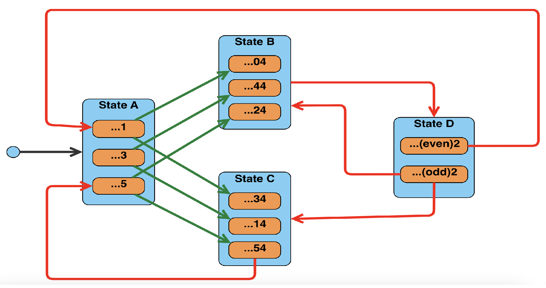
Figure 2.
Simplified version of FSM.

Figure 3.
HMM with the states corresponding to the simple cycles.
Disclaimer/Publisher’s Note: The statements, opinions and data contained in all publications are solely those of the individual author(s) and contributor(s) and not of MDPI and/or the editor(s). MDPI and/or the editor(s) disclaim responsibility for any injury to people or property resulting from any ideas, methods, instructions or products referred to in the content. |
© 2025 by the authors. Licensee MDPI, Basel, Switzerland. This article is an open access article distributed under the terms and conditions of the Creative Commons Attribution (CC BY) license (http://creativecommons.org/licenses/by/4.0/).
Copyright: This open access article is published under a Creative Commons CC BY 4.0 license, which permit the free download, distribution, and reuse, provided that the author and preprint are cited in any reuse.


