Submitted:
27 July 2025
Posted:
28 July 2025
You are already at the latest version
Abstract
This study compares PID and adaptive control algorithms for stabilizing the crankshaft speed of a diesel engine. Key performance metrics — response time, overshot and steady-state error — were analysed to evaluate control effectiveness. Experiments were conducted on a dynamometer test bench with variable mechanical loads introduced via alternator load adjustments. All tests were performed at a constant crankshaft speed using National Instruments measurement equipment and custom LabVIEW-based software for real-time monitoring. The analysis included four algorithms, among them a novel adaptive control strategy developed by authors. Statistical methods were used to assess performance differences. Results show that the proposed adaptive algorithm significantly improved control performance: approximately 20% in response time, 15% in overshoot, and 10% in error relative to the PID and covariance-based benchmarks. These findings highlight the potential of adaptive control in applications such as air-fuel ratio regulation, turbocharger pressure control, knock detection, and fuel optimisation.
Keywords:
diesel engine control
; adaptive control
; PID controller
; crankshaft speed stabilization
; control algorithm comparison
1. Introduction
Precise control of diesel engine crankshaft speed plays an important role in many engineering applications, including transportation, power generation, and unmanned systems [1]. Maintaining stable crankshaft speed under changing external loads and environmental conditions is essential to ensure adequate performance, fuel efficiency, and compliance with emission requirements [2]. Classic control strategies, such as proportional-integral-derivative (PID) controllers, are commonly used in combustion engine systems due to their simplicity of implementation and sufficient effectiveness under steady-state conditions [3]. However, their effectiveness can be significantly reduced in the event of dynamic disturbances or changes in system parameters. Unlike PID controllers, adaptive algorithms allow for real-time modification of control parameters in response to changing operating conditions and model uncertainties. Among them, promising approaches include adaptive covariance methods and multi-model strategies, which enable learning based on system responses and better adaptation to system nonlinearities and variable characteristics [4]. Such approaches are particularly important in applications where rapid load changes or mechanical component ageing occur.
Currently, work is underway on the use of various types of algorithms in the control of diesel engines [5,6,7,8], which prove that modern crankshaft speed control methods – such as TDOF PID, fuzzy PID, MPC, and PSO-fuzzy PID supported by UKF filtering – significantly outperform classic PID controllers in terms of response crankshaft speed, disturbance suppression, and stability under variable loads and system nonlinearities. The authors of those publications also emphasize the importance of accurate system modelling and simplified tuning of controller parameters, which, in combination with simulation tests, confirms the high effectiveness and ease of adaptation of the proposed solutions in various industrial applications.
Other studies show the possibility of eliminating fluctuations in the engine crankshaft speed signal. Article [9] presents a modified active disturbance rejection control (ADRC) algorithm based on a nonlinear scaling function (SARESO), dedicated to precise crankshaft speed control of diesel engines. The main achievements include the development of a method that improves disturbance suppression while reducing sensitivity to measurement noise. Simulations showed a significant performance improvement: disturbance suppression capability increased by 34.7 % (relative to the maximum deviation of speed from the target value), and the amplitude of control signal fluctuations in steady state was reduced by 43.6 % compared to existing ADRC controllers.
Engine crankshaft speed control is also important due to vibrations. For example, the authors of article [10] described the problem of torsional vibrations of the shaft coupled with the crankshaft speed control system of a diesel engine, which in real conditions led to crankshaft speed fluctuations of 20 rpm at a nominal crankshaft speed of 540 rpm. The proposed and validated simulation model, which took into account the deformable torsional vibrations of the shaft, showed crankshaft speed fluctuations of up to ± 21 rpm, in contrast to the simplified rigid shaft model, which showed only about 3 rpm. The research confirmed that ignoring vibration coupling results in an inaccurate picture of engine dynamics, which is crucial for designing effective adaptive algorithms in crankshaft speed control.
Excessive vibration values can lead to resonance. The authors of publication [11] presented a strategy for controlling the crankshaft speed of a diesel engine aimed at suppressing resonances in the drive system, which limit the effectiveness of traditional RQV crankshaft speed controllers, leading to wheel speed oscillations. The proposed method, based on a model that takes into account the dynamics of the drive system, effectively reduces resonance and the “vehicle shuffle” phenomenon, significantly improving response and reducing wheel speed overshoot compared to standard RQV control. Tests on a Scania 124L truck, in the engine crankshaft speed range from 1100 to 1900 rpm, confirmed the effectiveness of active vibration damping, which is key to improving driving comfort and vehicle dynamics.
The literature also includes studies on, among other things, the application of an innovative, phenomenological-based, and non-invasive method of estimating Indicated Mean Effective Pressure (IMEP) for marine diesel engines, based on instantaneous crankshaft speed signals [12]. Experimental validation confirmed the high accuracy of the method, showing a maximum error of 0.47 bar and an average error of 0.005 bar at 50 % load, which surpasses traditional pressure sensors by eliminating durability and interference issues, without the need for prior knowledge of the engine characteristics. The results of this research are particularly important as they confirm the validity of using the algorithm under variable load conditions.
Other types of research concern not only diesel engines, but also other types of propulsion systems. Article [13] presents a method for real-time optimisation of variable rotor speed for helicopters with a coaxial drive system, based on the adaptive AdamDNN-PSM model and the ASRUKF estimator, which significantly improves the accuracy of the onboard model and engine status tracking. The main result is an effective reduction in fuel consumption during patrol flights and an increase in the overall efficiency of the propulsion system, with the possibility of operating in the rotor speed range from 360 to 446 rpm. This approach, drawing on the concept of variable rotor speed, enables a potential reduction in power demand of more than 10 % with only a 15 % reduction in rotor speed. Similar studies are being conducted for UAVs [14]. Adaptive speed control techniques are also used to control electric motors [15,16,17], confirming their versatility. In addition, adaptive control can also be used to control the speed of Motor Hydrostatic Drive Powertrains in order to reduce energy consumption [18].
The literature also includes the application of algorithms for idle speed control. For example, publication [19] presents nonlinear model predictive control (NMPC) with the Firefly algorithm (FA) for regulating the idle speed of a car engine, implemented on an FPGA platform. The system is also characterised by fast response time and high stability, which positions it as an effective alternative to traditional PID algorithms and other adaptive methods in the context of engine crankshaft speed control.
Mechanical methods of controlling engine crankshaft speed are also used, such as those described in the article [20], which presents the concept and validation of a balancing cam mechanism designed to stabilize momentary fluctuations in torque and crankshaft speed in internal combustion engines as an alternative to traditional flywheels. Numerical simulations showed a reduction in crankshaft speed fluctuations of 83 % and torque fluctuations of 84 %, while experimental verification on a real engine confirmed reductions of 78 % and 75 %, respectively. These results demonstrate high efficiency in stabilising engine dynamics in the range of 1500 to 3500 rpm, which has significant implications for precise crankshaft speed control in the context of comparisons with PID and adaptive algorithms.
Other articles describe methods of applying machine learning to engine crankshaft speed control. Article [21] compares the implementation of reinforcement learning (RL) with the Deep Q-Network (DQN) algorithm and traditional PID control in terms of regulating the idle speed of an internal combustion engine. The results of simulation and experimental studies showed the superiority of RL-based control in reducing crankshaft speed fluctuations, improving engine efficiency, and optimizing fuel consumption, achieving an average improvement of 2 grams per minute. It has been proven that the RL controller is more accurate and precise in maintaining the set speed, as confirmed by lower SAE, MAE, MSE, and RMSE error values compared to PID.
Similarly, article [22] presents an innovative method for designing a controller for a wide-range variable cycle engine, based on deep reinforcement learning (DRL) with a DDPG algorithm, which effectively addresses the limitations of traditional PID controllers in complex operating conditions. The main results of the simulations, carried out for typical flight scenarios, showed that while the DRL controller effectively tracks the set speed values and stabilises the engine, the conventional PID controller proved unable to achieve stabilization. This confirms the significant advantage of adaptive DRL algorithms in the context of multi-variable engine crankshaft speed control.
Similar research is presented in the article [23], which describes a method for multi-objective real-time optimization of the combustion process in a diesel engine, integrating model predictive control (MPC) with reinforcement learning (RL) for synergistic optimisation of NOx emissions and indicated mean effective pressure (IMEP) by regulating rail pressure and injection timing. It has been shown that traditional control strategies are insufficient under transient conditions. The proposed approach, which uses samples from MPC to train RL, significantly improved the stability and efficiency of learning, resulting in a 16 % reduction in NOx emissions and a 0.32 % increase in IMEP in experimental validation, confirming its effectiveness in multi-objective real-time optimization.
Considering the above analysis of the state of knowledge, it seems reasonable to undertake work comparing four strategies for regulating the crankshaft speed of a diesel engine: a classic PID controller, an adaptive covariance algorithm, an adaptive controller with a single model, and an adaptive strategy with three competing controllers. Experimental research was conducted on a dynamometer powered by an Andoria ADCR engine, subjected to sudden changes in electrical load. The analysis covered the time courses of engine crankshaft speed and accelerator pedal position based on ten repetitions of each test. The work aims to evaluate the effectiveness, response speed, and stability of each control strategy under identical test conditions. The results obtained are intended to provide practical guidance on the selection and implementation of appropriate control algorithms in diesel engine applications where high precision and resistance to external disturbances are required.
2. Materials and Methods
The article presents four strategies for controlling the crankshaft speed of a diesel engine, three of which are the authors' own proposals:
- PID control,
- adaptive covariance algorithm,
- adaptive algorithm with a single controller,
- adaptive algorithm with three controllers (competitive).
2.1. PID Algorithm
Maintaining a stable engine crankshaft speed is crucial for its efficiency and safety. For this purpose, a PID controller can be used, in which the engine crankshaft speed is the controlled by the accelerator pedal position value. The purpose of the controller is to minimise the error between the set constant crankshaft speed and actual crankshaft speed.
The PID algorithm operates on the basis of three components:
- Proportional (Kp) – corresponding to the current error,
- Integrating (Ki) – taking into account the cumulative error over time,
- Derivative (Kd) – responding to the rate of change of the error.
The regulator output is described by Equation 1, and its block diagram is shown in Figure 1 (a).
The selection of Kp, Ki, and Kd parameters is based on methods such as Ziegler-Nichols or adaptive techniques. In the implementation of the algorithm, the current crankshaft speed is measured, the error is calculated, and then each PID term and the final control signal that determines the position of the accelerator pedal are calculated. In practice, especially in a dynamic working environment, the Ki and Kd terms can impair stability: the Kd term amplifies high-frequency disturbances, and excessive influence of the Ki term can lead to overshoot. Preliminary tests on a dynamometer have shown that in such an application, the Kp controller alone provides simpler and more stable control. The block diagram is shown in Figure 1 (a).
2.2. Adaptive Covariance Algorithm
The adaptive covariance algorithm is an advanced control method that allows for dynamic adjustment of control parameters in real time. Unlike classic controllers, this algorithm can “learn” and remember information about the control object, which is particularly important for diesel engine control under changing operating conditions. The algorithm consists of two main parts: an observer and a controller, operating in parallel. It uses the so-called forgetting factor β, which controls the speed of adaptation – the closer to 1, the faster but less accurate the response; lower values provide greater precision at the expense of response delay. In the algorithm, the engine crankshaft speed y(t) is controlled by the position of the accelerator pedal u(t). During system operation, the control error e(t) is calculated, and then the adaptation coefficients θ₁, θ₂ and the elements of the covariance matrix are updated. In the next steps, the updated accelerator pedal position u(t+1) is determined. Initialization involves assigning initial parameter values (e.g., θ₁ = 1, β = 0.99) and adaptive coefficient limits. The main calculation loop includes measuring input and output signals, calculating estimators, correcting parameters, and updating control. Thanks to dynamic adaptation, the covariance algorithm can better respond to changing operating conditions, such as changing blade loads or wind gusts, making it an attractive solution for the control of diesel engine. The block diagram is shown in Figure 1 (b).
2.3. Adaptive Algorithm with a Single Controller
In order to ensure stable and dynamic crankshaft speed control, an adaptive control algorithm based on a single controller was also tested. This algorithm allowed for automatic adjustment of control parameters in response to changing operating conditions of the drive system, such as load fluctuations. The algorithm works by continuously correcting a single coefficient that defines the relationship between the control signal (accelerator pedal position) and the resulting engine crankshaft speed. Deviations of the actual engine crankshaft speed from the set value cause automatic adjustment of this coefficient, which influences subsequent control decisions. The most important element of the algorithm is the adaptation coefficient β, which is modified during engine operation. Initially, it takes a base value, but from the very first moments of operation, it begins to adapt to the current conditions. This makes it possible to maintain the set speed even in a dynamically changing environment. To ensure a balance between response speed and stability, the algorithm uses a so-called forgetting function. It is based on a forgetting coefficient, which determines the extent to which the controller “remembers” previous conditions. A high value of this coefficient means that the algorithm responds slowly to changes but operates stably. A low value ensures a quick response, at the cost of greater sensitivity to temporary disturbances. The algorithm operates cyclically. At each time step, the current engine crankshaft speed and accelerator pedal position are measured. Based on this, the algorithm estimates whether the current control level was appropriate. If not, it updates its adaptation coefficient, which is then used to calculate a new control value. The advantage of this approach is its simplicity and the lack of need for manual tuning of parameters during operation. The algorithm responds independently to changes in load or external conditions, which makes it particularly useful in systems that are difficult to access or operate in unstable conditions. It can also be extended with additional mechanisms, such as filtering measurement disturbances or limiting control values to ensure system safety. The block diagram is shown in Figure 2 (a).
2.4. Adaptive Algorithm with Three Controllers (Competitive)
A competitive algorithm is an advanced method of adaptive control based on the simultaneous operation of three controllers with different response dynamics. Each controller has its forgetting coefficient, which determines the rate at which it adapts to changing conditions. This approach allows for flexible response to various drive system operating scenarios, combining the advantages of rapid adaptation and stable operation.
The algorithm uses:
- aggressive regulator – reacts quickly to changes, but may be less stable,
- balanced regulator – a compromise between speed of adaptation and stability,
- conservative regulator – changes slowly, but provides high stability.
At any given moment, the algorithm evaluates the effectiveness of individual controllers based on their ability to predict the actual engine crankshaft speed. Based on this comparison, the controller that currently best reflects reality is selected, and its control signal is used to control the system. Because all three controllers operate in parallel, it is possible to dynamically switch control between them in real time. This allows for automatic adaptation to changing operating conditions, such as sudden load changes. Each controller independently updates its parameters based on current measurements of crankshaft speed and accelerator pedal position. It then calculates its control value proposal and predicts the crankshaft speed that this value will cause. The controller that predicts the closest result to the actual set value is selected for control in a given step. This approach offers high resistance to single model errors. If any of the controllers cease to accurately reflect the dynamics of the object, their signal is not used for control, and their parameters can continue to learn in the background. The use of such a control strategy is particularly justified in environments where operating conditions change rapidly and accuracy and stability of operation are critical. The algorithm can be used, among other things, to regulate the rotational speed of helicopter blades, torque in diesel engines, or renewable energy systems—anywhere where flexible, self-adjusting control is required. The block diagram is shown in Figure 2 (b).
2.5. Research Test Bench
The subject of the study was the Andoria ADCR engine, manufactured by Andoria-Mot Sp. z o.o., which complies with the Euro 4 emission standard. It is a compression ignition engine equipped with a Common Rail fuel supply system and a turbocharger with an intercooler. The engine has a displacement of 2636 cm³, generates 85 kW of mechanical power at a crankshaft speed of 3700 rpm, and achieves a maximum torque of 250 Nm in the speed range from 1800 to 2200 rpm. The basic technical data of the engine are presented in Table 1.
The tests were carried out at a test station located in the laboratory of the Department of Thermodynamics, Fluid Mechanics, and Aircraft Propulsion at the Lublin University of Technology (Innovation and Advanced Technology Center building). The test stand consists of two main parts: a mechanical system and control and data recording systems. The main component of the mechanical system is the Andoria ADCR combustion engine, coupled with an electronically controlled EMX–200/6000 electrodynamic brake manufactured by Elektromex Centrum [26]. The drive unit was mounted on a frame, and torque is transmitted via a Cardan shaft with a Zerkopol damping clutch. The control system includes a factory-installed Bosch EDC16C39-6.H1 controller, which allows control of engine operating parameters based on input signals such as accelerator pedal position, torque, power etc. The measurement data included, among others, crankshaft speed, oil temperature and pressure, exhaust gas temperature, air pressure and flow, and current values from transducers. The EMX brake measurement and control system was based on a CAN bus and included an ATMX2070 controller and an ATMX2011-4 console. The brake was equipped with a water cooling system and had a maximum power of up to 200 kW. A view of the test stand is shown in Figure 3.
The electric brake was controlled using the ParmSuite application in conjunction with the ATMX2011 console (Automex Sp. z o.o.), which enabled monitoring of torque, crankshaft speed, and accelerator pedal position. The test engine was equipped with independent liquid, oil, and intake air cooling systems, working with a central heat exchanger (400 kW) and a heat accumulator. The liquid cooling system included, among other things, exchangers, a pump, a thermostat, and an expansion tank. The lubrication system consisted of two oil pumps, three heat exchangers, sensors, and a filter. The intake and exhaust system included exchangers, a silencer, a throttle, a filter, and sensors (temperature, pressure, MAS). The fuel system was built using Bosch components: injectors, a pump, and a common rail. The electrical load system included 20 pcs. of 24 V/100 W bulbs and a 180556/24V contactor from Littelfuse [27], controlled by an HDR-150-24 (Mean Well) power supply [28]. The currents were measured using HTA1 (200 A) and HTA2 (300 A) transducers [29,30], powered by DR-60-12 [31]. The crankshaft speed, torque, power, and accelerator pedal position were recorded at a frequency of 0.02 s using a CAN bus and an NI USB-8473 adapter. Other parameters (current, voltage, pedal position) were measured using NI-9215, NI-9411, and NI-9264 cards [32,33,34] embedded in CompactDAQ9174 and cRIO-9024 housings [35], powered by PULS QS10.241. The Relpol RM84 relay enabled switching of pedal control between the computer and the dynamometer system. The station enabled the recording of: crankshaft speed, torque, brake power, pedal position, currents (alternator–battery, battery–load) and contactor voltage. The measurement was carried out in unconditioned environmental conditions (temperature 26 ± 1°C, pressure 100 ± 2 kPa, humidity 45 ± 5%), over one day and using a single batch of fuel. The measurement system diagram is shown in Figure 4.
A scenario corresponding to a power difference of 5.298 % was selected for analysis. It was determined that this percentage change in power should be reproduced in laboratory conditions on a dynamometer. The tests were carried out using the previously described test rig. Preliminary tests were performed to precisely determine the electrical load generated by the load system. For both the preliminary tests and the actual tests, a representative engine crankshaft speed of 2000 rpm was adopted, at which the Andoria ADCR engine operates stably. For safety reasons and to reduce wear on the unit, the full power of the engine was not used. During the tests, it was determined that applying an electrical load with a nominal power of 1 kW (a set of 20 incandescent bulbs) resulted in an actual power consumption of 850 W.
The Delphi alternator, mounted on the Andoria ADCR engine using a multi-ribbed belt (4PK948) with a ratio of 2.5, achieves an efficiency of converting mechanical energy into electrical energy of approx. 62.8 % at a rotational speed of 5000 rpm (for an engine crankshaft speed of 2000 rpm). Previous studies have shown that the efficiency of similar alternators ranges from 50 % to 80 %, and for the analysed laboratory system, it was approximately 64%. At a nominal load of 1 kW, the actual mechanical power requirement was 1.353 kW. These conditions were reproduced on the test bench, taking into account a scenario of increased power demand (5.298 %), which corresponds to the following parameters: 2000 rpm, torque 120.61 Nm, and power 25.26 kW.
3. Results and Discussion
This chapter presents the results of the test bench tests, divided into four subsections, covering: PID control, adaptive covariance control, adaptive control with a single controller, and adaptive control with three controllers (competitive). In each case, the time histories of the crankshaft speed and accelerator pedal position were tested presented for three representative controller settings. Each test lasted 150 seconds and included two-step load transitions: activation at 30 seconds and deactivation at 90 seconds. An additional 60 seconds between tests allowed the system to stabilize. Ten repetitions were performed for each test, and the average errors were calculated as the average values from these tests.
The first value analyzed was Response time RT. It was defined as time that elapses from the moment the load is applied until the engine crankshaft speed reaches and remains within the ± 2% band of the new set value.
Overshot OV was the maximum deviation of the output signal value above the new set value, expressed as a percentage:
where:
- is the maximum crankshaft speed value after responding to the disturbance,
- is the new steady-state value.
Steady-state error SSE was defined as the average absolute deviation from the set values measured after 10 seconds of stabilization.
where:
- is the actual crankshaft speed value,
- is the new steady-state value,
- is the number of measurements.
All results values are presented in Table 2. The following sections present one example graph from each control strategy showing the engine crankshaft speed signal and the accelerator pedal position signal for example set values.
3.1. Test Results for the PID Control
Figure 5 shows the time course of crankshaft speed and accelerator pedal position for PID control with the Kp = 0.00125. The values shown in the graph represent the average value from 10 consecutive trials carried out during the tests.
The empirical results underscore the inherent limitations of the PID controller in dynamic environments characterized by abrupt load perturbations, such as those induced by alternator adjustments. For the PID variants (corresponding to configurations Kp = 0.00125, Kp = 0.00250, Kp = 0.00500), the mean response times ranged from 2.5 to 4.1 seconds, with overshoots of 1.02% to 1.63% and steady-state errors of 0.09 to 0.27 rpm. While these metrics indicate acceptable performance in quasi-static conditions, the PID's fixed gain structure (tuned via Ziegler-Nichols or similar heuristics) exhibits suboptimal adaptability to nonlinearities inherent in diesel engine dynamics, including fuel injection delays, turbocharger lag, and torsional vibrations. This corroborates prior literature [6,7], where fixed-parameter controllers fail to mitigate resonance-induced fluctuations exceeding ±20 rpm, potentially leading to increased fuel consumption and emissions.
3.2. Research Results for Adaptive Covariance Control
Figure 6 shows the time course of crankshaft speed and accelerator pedal position for adaptive covariance control with the β = 0.99. The values shown in the graph represent the average value from 10 consecutive trials carried out during the tests.
In contrast, the adaptive covariance control algorithm (corresponding to configurations β = 0.50, β = 0.96, β = 0.99) demonstrates enhanced robustness through real-time parameter adjustment via a forgetting factor β, yielding response times of 4.9 to 6.3 seconds, overshoots of 2.57% to 4.36%, and errors of 0.12 to 0.17 rpm. This method's ability to "learn" system uncertainties—such as varying load torques—via covariance matrix updates aligns with adaptive disturbance rejection principles [9], reducing sensitivity to measurement noise by up to 43.6% compared to non-adaptive baselines. However, the algorithm's reliance on a single adaptive coefficient introduces a trade-off between convergence speed and precision, particularly evident in higher β values (e.g., 0.99), where transient oscillations persist longer due to aggressive adaptation.
3.3. Research Results for Adaptive Control with a Single Controller
Figure 7 shows the time course of crankshaft speed and accelerator pedal position for adaptive control with a single controller with the β = 0.99. The values shown in the graph represent the average value from 10 consecutive trials carried out during the tests.
The adaptive control with a single controller (corresponding to configurations β = 0.50, β = 0.96, β = 0.99) further refines this paradigm by employing a solitary adaptive gain updated based on error residuals, achieving response times of 3.8 to 5.2 seconds, overshoots of 2.13% to 4.28%, and notably low steady-state errors of 0.01 to 0.06 rpm. This configuration's simplicity facilitates implementation in embedded systems, such as engine control units (ECUs), and exhibits superior steady-state accuracy, attributable to its continuous recalibration of the input-output relationship (accelerator pedal position to rpm). Nonetheless, its performance degrades under rapid load transients, as the single-model framework lacks redundancy to handle multimodal system behaviors.
3.4. Research Results for Adaptive Control with Three Competing Controllers
Figure 8 shows the time course of crankshaft speed and accelerator pedal position for adaptive control with three competing controllers with the β = 0.97. The values shown in the graph represent the average value from 10 consecutive trials carried out during the tests.
The proposed adaptive regulator with three competing controllers (corresponding to configurations β = 0.90, β = 0.95, β = 0.97) emerges as the most efficacious strategy, integrating three parallel regulators with distinct forgetting factors (aggressive, balanced, and conservative) to dynamically select the optimal model based on predictive error minimization. This yields the lowest response times (1.7 to 2.9 seconds), overshoots (0.77% to 1.62%), and steady-state errors (0.02 to 0.04 rpm), representing reductions of approximately 20% in response time, 15% in overshoot, and 10% in error relative to the PID and covariance-based benchmarks. The competitive mechanism mitigates the pitfalls of single-model adaptation by enabling seamless switching among models, akin to ensemble methods in reinforcement learning [21,22], thereby enhancing disturbance rejection and stability in the presence of nonlinearities like vehicle shuffle [11] or IMEP variations [12,23]. Statistical validation across repetitions confirms these improvements with high confidence, as evidenced by reduced standard deviations in error metrics.
4. Conclusions
These findings affirm the superiority of adaptive control paradigms over classical PID in diesel engine crankshaft speed regulation, particularly for applications demanding high precision amid variable loads, such as unmanned aerial vehicles (UAVs) [14], marine propulsion [8,17], or hydrostatic drives [18]. The proposed competitive algorithm's potential extends to ancillary engine functions, including air-fuel ratio optimization, turbocharger boost control, knock mitigation, and fuel efficiency enhancement, potentially reducing NOx emissions by 16% and improving IMEP by 0.32% as suggested by synergistic MPC-RL approaches [23]. Future research should explore hybrid integrations with deep reinforcement learning (e.g., DDPG or DQN) for broader operational envelopes and real-time hardware-in-the-loop validation on production engines. Moreover, sensitivity analyses to β parameterization and noise filtering (e.g. via UKF [7]) could further refine the algorithm's deployability in industrial settings.
Author Contributions
Conceptualization, P.M., M.W., A.G. and M.A.Z.; methodology, P.M. and M.W.; software, P.M.; validation, M.W.; formal analysis, A.G. and M.A.Z.; investigation, P.M. and M.W.; resources, P.M.; data curation, M.W.; writing—original draft preparation, P.M.; writing—review and editing, P.M., A.G., M.W. and M.A.Z.; visualization, P.M.; supervision, M.W. and A.G.; project administration, P.M.; funding acquisition, P.M. All authors have read and agreed to the published version of the manuscript.
Funding
The project/research was financed in the framework of the Lublin University of Technology funds conducting scientific activities FD - discipline fund, funded by the Polish Ministry of Science and Higher Education - Article 365 (2) of July 20, 2018.
Data Availability Statement
The data presented in this study are available on request from the corresponding author.
Conflicts of Interest
The authors declare no conflicts of interest.
Abbreviations
The following abbreviations are used in this manuscript:
| ADRC | Active Disturbance Rejection Control |
| APP | Acceleration Pedal Position |
| ASRKF | Adaptive Square Root Kalman Filter |
| DDPG | Deep Deterministic Policy Gradient |
| DNN-PSM | Deep Neural Network Propulsion System Model |
| DQN | Deep Q-Network |
| DRL | Deep Reinforcement Learning |
| FA | Firefly Algorithm |
| FPGA | Field-Programmable Gate Array |
| IMEP | Indicated Mean Effective Pressure |
| MAE | Mean Absolute Error |
| MPC | Model Predictive Control |
| MPC | Model Predictive Control |
| MSE | Mean Squared Error |
| NMPC | Nonlinear Model Predictive Control |
| PID | Proportional Integral Derivative |
| PSO | Particle Swarm Optimisation |
| RL | Reinforcement Learning |
| RMSE | Root Mean Squared Error |
| RPM | Rotation Per Minute |
| RQV | Regler Quer Verstellung |
| SAE | Sum of Absolute Errors |
| SARESO | Scaling Augmented Reduced-Order Extended State Observer |
| TDOF | Two Degree Of Freedom |
| UAV | Unmanned Aerial Vehicle |
| UKF | Untraceable Kalman Filter |
References
- Magryta, P.; Pietrykowski, K. Crankshaft geometry modification and strength simulations for a new design of diesel opposed-piston engine. Combustion Engines, 2023, 194(3), 123-128.
- Tucki, K.; Mruk, R.; Orynycz, O.; Botwinska, K.; Gola, A.; Bączyk, A. Toxicity of exhaust fumes (CO, NOx) of the compression-ignition (diesel) engine with the use of simulation, Sustainability 2019, 11(8), 2188.
- Magryta, P.; Grabowski Ł.; Barański, G.; Wendeker M., Toxic Emission During Road Tests of Urban Bus. Advances in Science and Technology. Research Journal 2023, 27(6), 16-26. [CrossRef] [PubMed]
- Tucki, K.; Mruk, R.; Orynycz, O.; Gola, A. The Effects of Pressure and Temperature on the Process of Autoignition and Combustion of Rape Oil and its Mixtures, Sustainability 2019, 11(12), 3451.
- Zeng, B.; Shen, Q.; Wang, G.; Wang, Y.; Zhao, Y.; He, S.; Yu, X. Research on Diesel Engine Speed Control Based on Improved Salp Algorithm. Processes 2023, 11. [CrossRef]
- Jiang, H.; Wang, D.; Cheng. J.; Li, P.; Ji, X.; Shen, Y.; Wu, M. Research on Speed Control Strategies for Explosion-Proof Diesel Engine Monorail Cranes. Actuators 2024, 13. [CrossRef]
- Fu, J.; Gu. S.; Wu. L.; Wang. N.; Lin, L.; Chen, Z. Research on Optimization of Diesel Engine Speed Control Based on UKF-Filtered Data and PSO Fuzzy PID Control. Processes 2025, 13. [CrossRef]
- So, G-B.; Jin, G-G.; Lee, C-H.; So, H-R.; Kim. D-J.; Ahn, J-K. TDOF PID Controller for Enhanced Disturbance Rejection with MS-Constraints for Speed Control of Marine Diesel Engine. J. Mar. Sci. Eng. 2024, 12.
- Zhou, Q.; Song, K.; Xie, H. Nonlinear Scaling Function based Active Disturbance Rejection Control for Diesel Engine Speed. IFAC PapersOnLine 2024, 58-29, 136-141. [CrossRef]
- Guo, Y.; Li, W.; Yu, S.; Han, X.; Yuan, Y.; Wang, Z.; Ma, X. Diesel engine torsional vibration control coupling with speed control system. Mechanical Systems and Signal Processing 2017, 94, 1-13. [CrossRef]
- Pettersson, M.; Nielsen, L. Diesel engine speed control with handling of driveline resonances. Control Engineering Practice 2023, 11, 319–328. [CrossRef]
- Ou, S.; Yu, Y.; Chen, G.; Hu, L.; Yang, J.; Ma, B. A control-oriented IMEP estimation method for a marine diesel engine based on crankshaft instantaneous speed. Measurement 2025, 248. [CrossRef]
- Song, J.; Wang, Y.; Ji, C.; Zhang, H. Real-time optimization control of variable rotor speed based on Helicopter/turboshaft engine on-board composite system. Energy 2024, 301. [CrossRef]
- Feng, Y.; Chen, T.; Liu, Q.; Zhao, H. Adapted Speed Control of Two-Stroke Engine with Propeller for Small UAVs Based on Scavenging Measurement and Modeling. Aerospace 2025, 12. [CrossRef]
- Zuo, Y.; Zhu, S.; Cui, Y.; Liu, C.; Lin, X. Adaptive PI Controller for Speed Control of Electric Drives Based on Model Reference Adaptive Identification. Electronics 2024, 13. [CrossRef]
- Kroics, K.; Bumanis, A. BLDC Motor Speed Control with Digital Adaptive PID-Fuzzy Controller and Reduced Harmonic Content. Energies 2024, 17. [CrossRef]
- Zhang, X.; Xu, X.; Xu, X.; Hou, P.; Gao, H.; Ma, F. Intelligent Adaptive PID Control for the Shaft Speed of a Marine Electric Propulsion System Based on the Evidential Reasoning Rule. Mathematics 2023, 11. [CrossRef]
- Wang, H.; Zhang, Y.; An, Z.; Liu. R. An Energy-Effi cient Adaptive Speed-Regulating Method for Pump-Controlled Motor Hydrostatic Drive Powertrains. Processes 2024, 12.
- Al-Jarrah, M. A.; Jarrah, A.; Alawaisah A. Automotive engine idle speed controller: Nonlinear model predictive control utilizing the firefly algorithm. Computers and Electrical Engineering 2023, 108. [CrossRef]
- Cardoso, D. S.; Fael, P. O.; Gaspar, P. D.; Espírito-Santo, A. Balancing Cam Mechanism for Instantaneous Torque and Velocity Stabilization in Internal Combustion Engines: Simulation and Experimental Validation. Energies 2025, 18. [CrossRef]
- Omran, I.; Mostafa, A.; Seddik, A.; Ali, M.; Hussein, M.; Ahmed, M.; Aly, Y.; Abdelwahab, M. Deep reinforcement learning implementation on IC engine idle speed control. Ain Shams Engineering Journal 2024, 15. [CrossRef]
- Ding, Y.; Wang, F.; Mu, Y.; Sun, H. Wide-Range Variable Cycle Engine Control Based on Deep Reinforcement Learning. Aerospace 2025, 12. [CrossRef]
- Chen, Z.; Ju, P.; Wang, Z.; Shi. L.; Deng, K. Research on multi-objective optimization control of diesel engine combustion process based on model predictive control-guided reinforcement learning method. Energy 2025, 325. [CrossRef]
- Magryta, P. Adaptacyjne sterowanie śmigłowcowym silnikiem Diesla. PhD. Thesis, 2024.
- Engine data sheet ADCR EURO4, ANDORIA-MOT Sp. z o.o.
- Operating and usage instructions for the EMX electric motor brake, Elektromex Centrum, 2008.
- Catalog card for contactor 180556/24V. https://www.littelfuse.com/ (accessed on 09 July 2025).
- HDR-150-24 power supply offer in the online store. https://www.zasilacze-meanwell.pl/4835-hdr-150-24-zasilacz-na-szyne-din-150w-24v-625a.html (accessed on 09 July 2025).
- HTA 200-S current transducer offer in the online store. https://pl.rs-online.com/web/p/transformatory-pradu/7315267 (accessed on 09 July 2025).
- HTR 300-SB current transducer offer in the online store. https://pl.rs-online.com/web/p/transformatory-pradu/0497299?searchId=02c0cce2-d36e-499f-b985-5f8dd7d043ff&gb=s (accessed on 09 July 2025).
- DR-60-12 power supply offer in the online store. https://www.zasilacze-meanwell.pl/1436-dr-60-12-zasilacz-na-szyne-din-60w-12v-45a.html (accessed on 09 July 2025).
- NI-9215 card offer in the online store. https://pl.farnell.com/ni/ 779138-01/voltage-input-module-16bit-100ksps/dp/3621386 (accessed on 09 July 2025).
- NI-9264 card offer in the online store https://pl.farnell.com/ni/779699-02/ni-9264-voltage-output-module/dp/3621552 (accessed on 09 July 2025).
- NI-9411 card offer in the online store. https://pl.farnell.com/ni/779005-01/ni-9411-digital-mod-c-series/dp/3621328 (accessed on 09 July 2025).
- cDAQ-9174 enclosure in online store. https://pl.farnell.com/ni/781157-01/chassis-4slot-compactdaq-system/dp/3621888 (accessed on 09 July 2025).
Figure 1.
Block diagram of algorithms for regulating the crankshaft speed of a diesel engine (a) PID algorithm; (b) Adaptive covariance algorithm [24].
Figure 1.
Block diagram of algorithms for regulating the crankshaft speed of a diesel engine (a) PID algorithm; (b) Adaptive covariance algorithm [24].
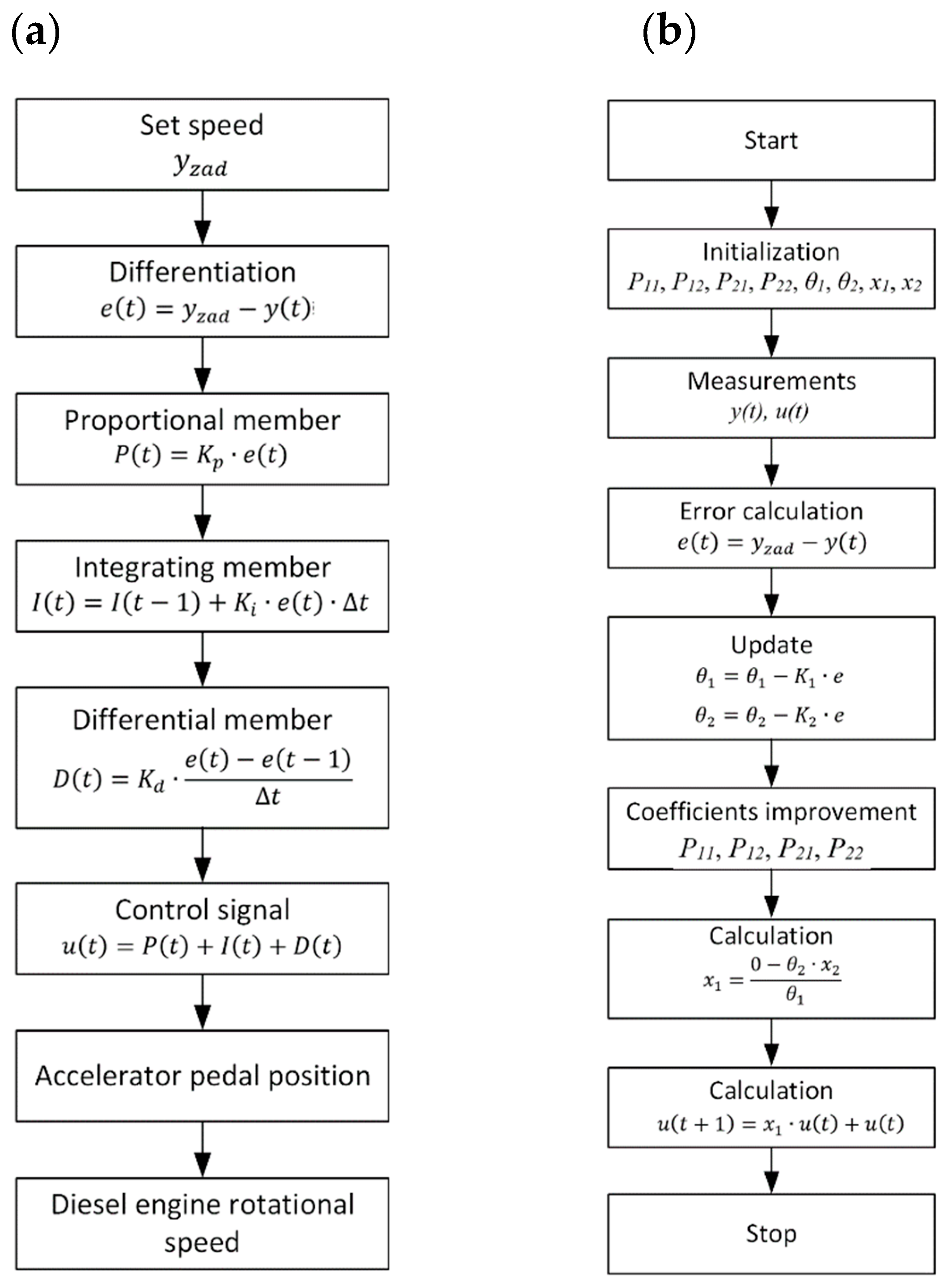
Figure 2.
Block diagram of algorithms for regulating the crankshaft speed of a diesel engine (a) Adaptive algorithm with a single controller; (b) Competitive adaptive algorithm [24].
Figure 2.
Block diagram of algorithms for regulating the crankshaft speed of a diesel engine (a) Adaptive algorithm with a single controller; (b) Competitive adaptive algorithm [24].
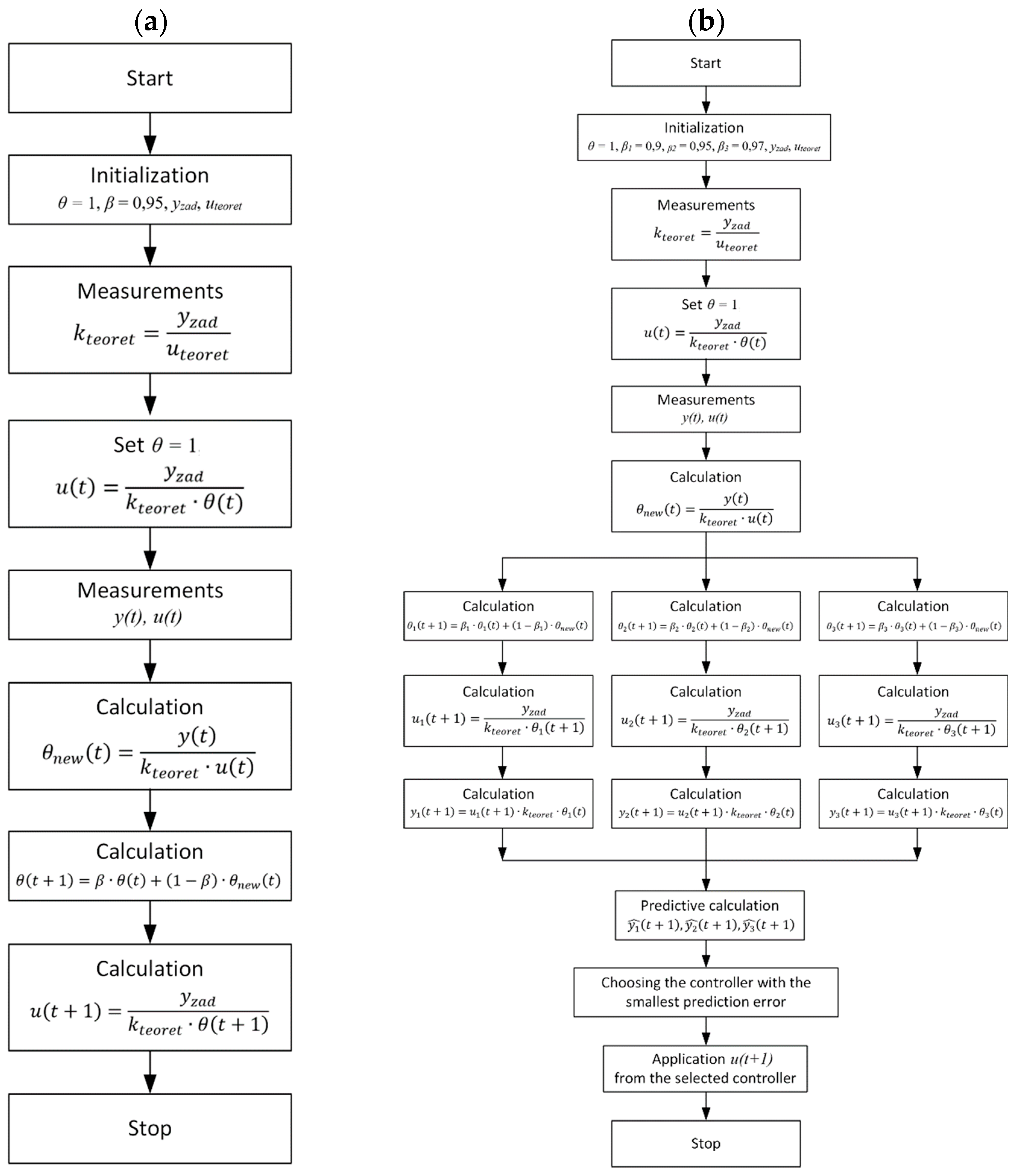
Figure 3.
Research test bench [24].
Figure 3.
Research test bench [24].
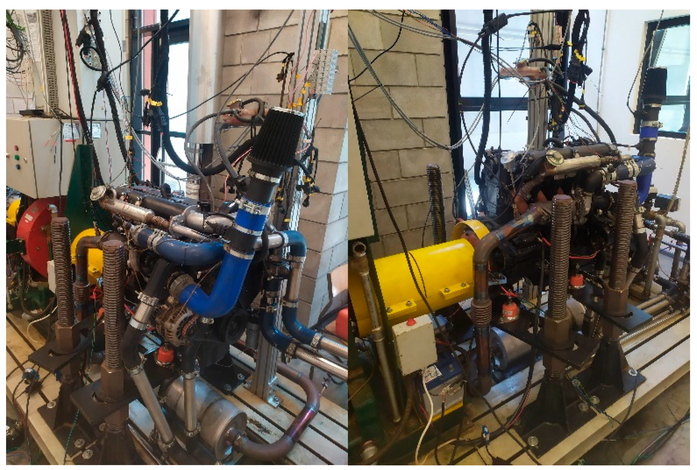
Figure 4.
Measurement system diagram [24].
Figure 4.
Measurement system diagram [24].
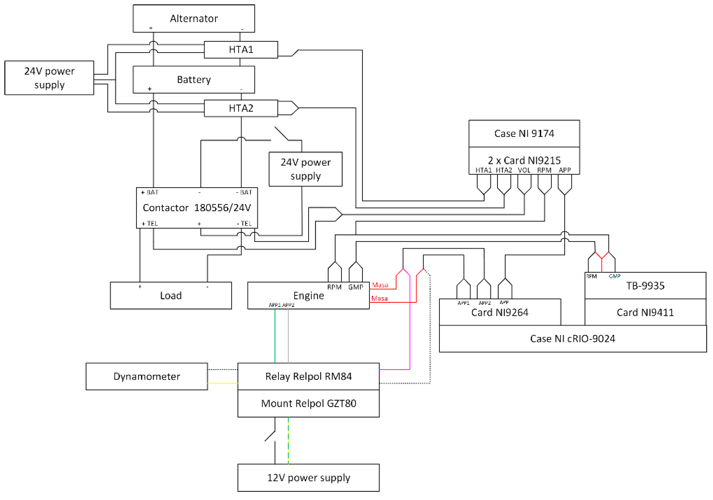
Figure 5.
Time course of crankshaft speed and accelerator pedal position for Kp = 0.00125.
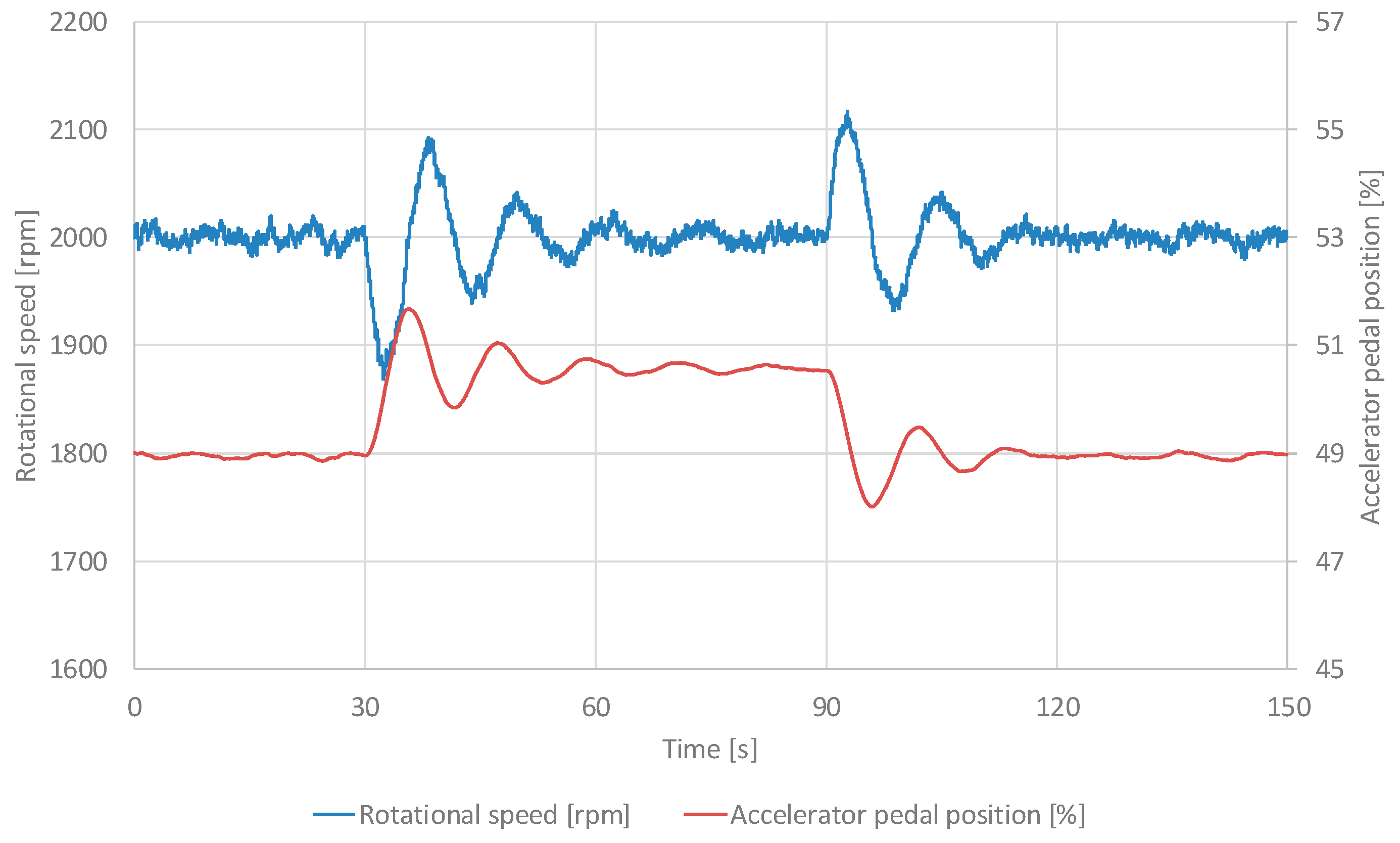
Figure 6.
Time course of crankshaft speed and accelerator pedal position for β = 0.99.
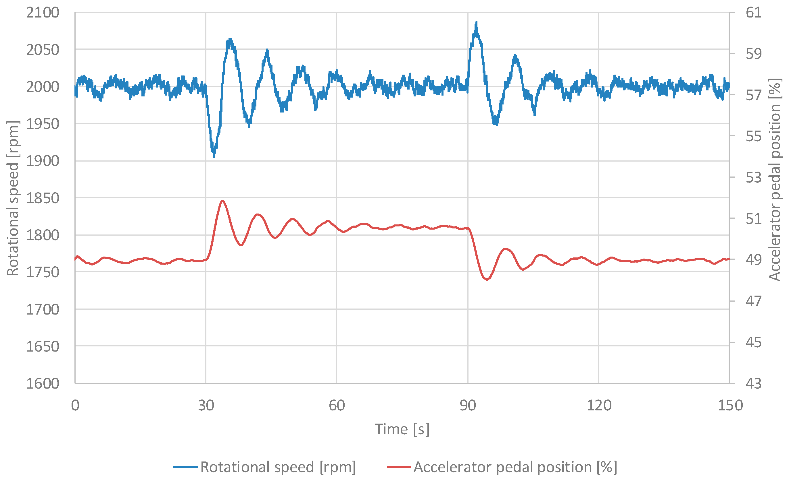
Figure 7.
Time course of crankshaft speed and accelerator pedal position for β = 0.99.
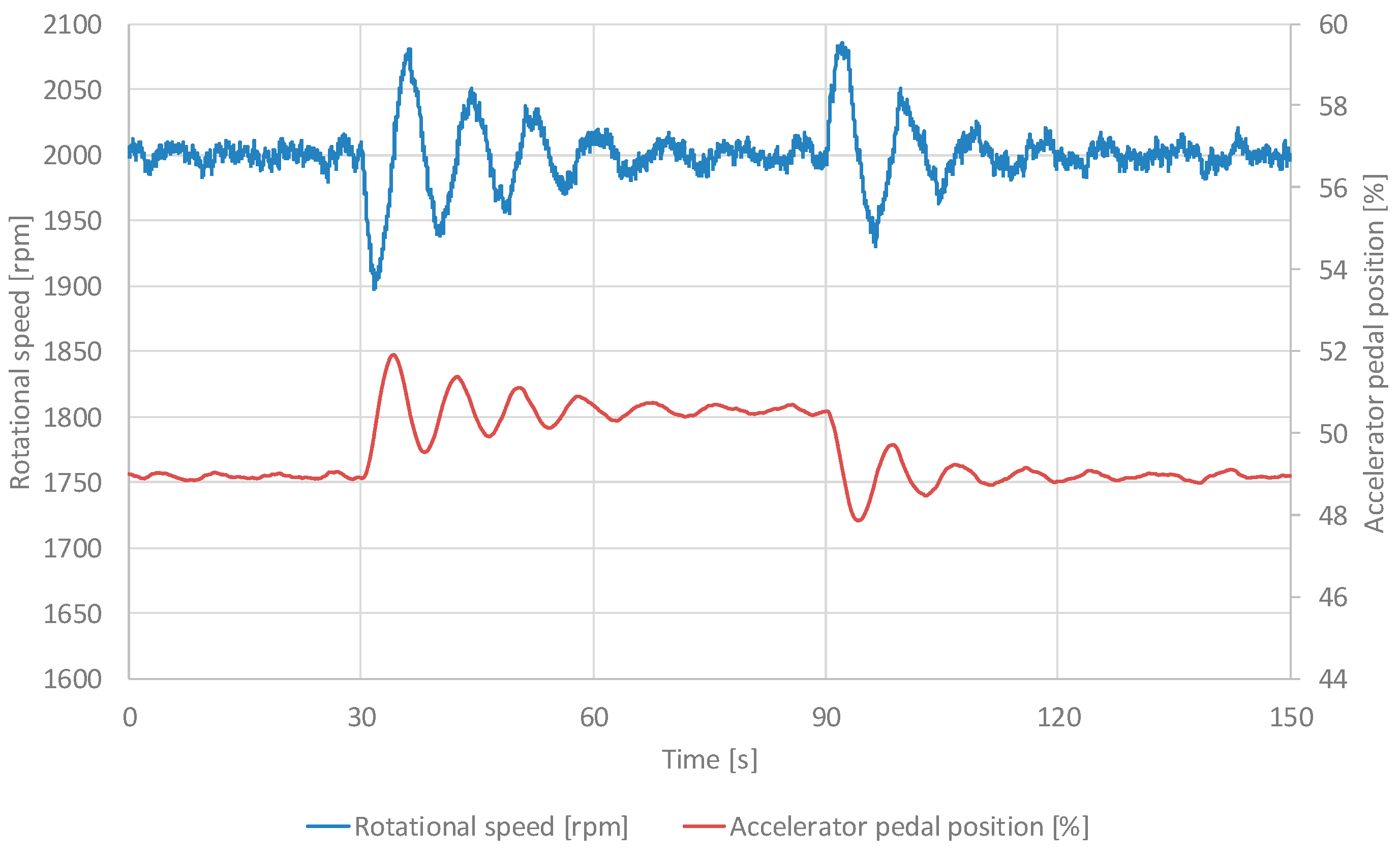
Figure 8.
Time course of crankshaft speed and accelerator pedal position for β = 0.97.
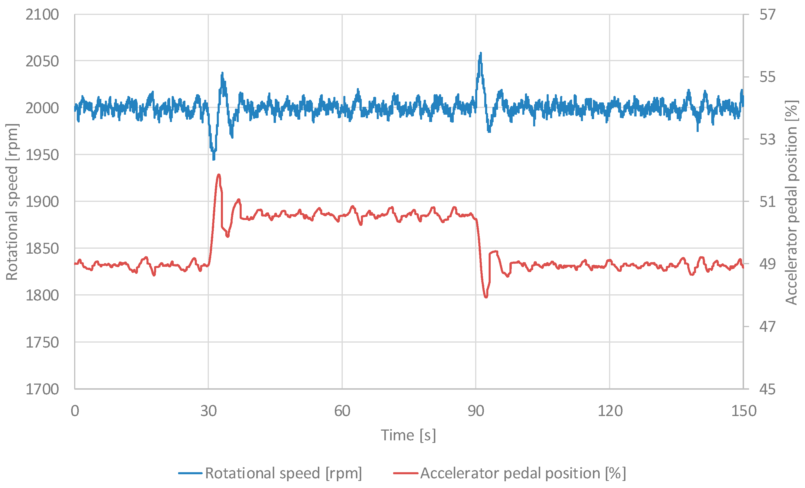

Table 1.
Basic technical data of the Andoria ADCR engine [25].
Table 1.
Basic technical data of the Andoria ADCR engine [25].
| Parameter | Value/Description |
| Designation | ADCR |
| Engine type | 4-stroke diesel, self-igniting, turbocharged |
| Number and arrangement of cylinders | 4, in-line, vertical |
| Cylinder diameter/piston stroke | 94 mm/95 mm |
| Cylinder displacement | 2,636 cm3 |
| Compression ratio | 17.5 |
| Fuel supply system | Common Rail system |
| Air supply system | turbocharged with intercooler |
| Net rated power according to ISO 1585 | 85 kW |
| Rated crankshaft speed | 3,700 rpm |
| Maximum net torque according to ISO 1585 | 250 Nm |
| Crankshaft speed at maximum torque | 1,800–2,200 rpm |
| Minimum idling speed | 750 rpm |
| Specific fuel consumption at maximum net engine torque according to ISO 1585 | 210 g/kWh |
| Fuel | diesel fuel |
| Type of timing | OHC |
| Engine start-up | 12V electric starter |
Table 2.
Results of the research.
| Test number | Set values | Response time RT [s] |
Overshot OV [%] |
Steady-state error SSE [rpm] |
| PID control | Kp = 0.00125 | 2.5 | 1.02 | 0.27 |
| Kp = 0.00250 | 3.2 | 1.06 | 0.13 | |
| Kp = 0.00500 | 4.1 | 1.63 | 0.09 | |
| Adaptive covariance control | β = 0.50 | 5.8 | 2.57 | 0.17 |
| β = 0.96 | 4.9 | 2.94 | 0.12 | |
| β = 0.99 | 6.3 | 4.36 | 0.13 | |
| Adaptive control with a single controller | β = 0.50 | 4.6 | 2.13 | 0.01 |
| β = 0.96 | 3.8 | 2.77 | 0.06 | |
| β = 0.99 | 5.2 | 4.28 | 0.02 | |
| Adaptive control with three competing controllers | β = 0.90 | 2.9 | 1.62 | 0.03 |
| β = 0.95 | 2.1 | 0.77 | 0.04 | |
| β = 0.97 | 1.7 | 0.84 | 0.02 |
Disclaimer/Publisher’s Note: The statements, opinions and data contained in all publications are solely those of the individual author(s) and contributor(s) and not of MDPI and/or the editor(s). MDPI and/or the editor(s) disclaim responsibility for any injury to people or property resulting from any ideas, methods, instructions or products referred to in the content. |
© 2025 by the authors. Licensee MDPI, Basel, Switzerland. This article is an open access article distributed under the terms and conditions of the Creative Commons Attribution (CC BY) license (http://creativecommons.org/licenses/by/4.0/).
Copyright: This open access article is published under a Creative Commons CC BY 4.0 license, which permit the free download, distribution, and reuse, provided that the author and preprint are cited in any reuse.


