
Submitted:
24 July 2025
Posted:
25 July 2025
You are already at the latest version
Abstract
In this paper, closed-form expressions for the variation of the expectation of a given function due to changes in the probability measure (probability distribution drifts) are presented. They unveil interesting connections with Gibbs probability measures, mutual information, and lautum information.
Keywords:
gibbs probability measures
; sensitivity
; distribution shifts
; variations of the expectation
1. Introduction
Let m be a positive integer and denote by the set of all probability measures on the measurable space , with being the Borel -algebra on . Given a Borel measurable function , consider the functional
which quantifies the variation of the expectation of the measurable function h due to changing the probability measure from to . These variations are often referred to as probability distribution drifts, in some application areas, see for instance [1,2] and [3]. The functional is defined when both integrals exist and are finite.
In order to define the expectation of when x is obtained by sampling a probability measure in , the structure formalized below is required.
Definition 1.
A family of elements of indexed by is said to be a conditional probability measure if, for all sets , the map
is Borel measurable. The set of all such conditional probability measures is denoted by .
In this setting, consider the functional
This quantity can be interpreted as the variation of the integral (expectation) of the function h when the probability measure changes from the joint probability measure to another joint probability measure , both in . This follows from (2) by observing that
Special attention is given to the quantity , for some , with being the marginal of the joint probability measure . That is, for all sets ,
Its relevance stems from the fact that it captures the variation of the expectation of the function h when the probability measure changes from the joint probability measure to the product of its marginals . That is,
1.1. Novelty and Contributions
This work makes two key contributions: First, it provides a closed-form expression for the variation in (1) for a fixed and two arbitrary probability measures and , formulated explicitly in terms of relative entropies. Second, it derives a closed-form expression for the expected variation in (2), again in terms of information measures, for arbitrary conditional probability measures , , and an arbitrary probability measure .
A further contribution of this work is the derivation of specific closed-form expressions for in (6), which reveal deep connections with both mutual information [4,5] and lautum information [6]. Notably, when is a Gibbs conditional probability measure, this variation simplifies (up to a constant factor) to the sum of the mutual and lautum information induced by the joint distribution .
Although these results were originally discovered in the analysis of generalization error of machine learning algorithms, see for instance [7,8,9,10,11], where the function h in (1) was assumed to represent an empirical risk, this paper presents such results in a comprehensive and general setting that is no longer tied to such assumptions. Also, strong connections with information projections and Pythagorean identities [12,13] are discussed. This new general presentation not only unifies previously scattered insights but also makes the results applicable across a broad range of domains in which changes in the expectation due to variations of the underlying probability measures are relevant.
1.2. Applications
The study of the variation of the integral (expectation) of h (for some fixed ) due to a measure change from to , i.e., the value in (1), plays a central role in the definition of integral probability metrics (IPMs)[14,15]. Using the notation in (1), an IPM results from the optimization problem
for some fixed and a particular class of functions . Note for instance that the maximum mean discrepancy is an IPM [16], as well as the Wasserstein distance of order one [17,18,19,20].
Other areas of mathematics in which the variation in (1) plays a key role is distributionally robust optimization (DRO) [21,22] and optimization with relative entropy regularization [8,9]. In these areas, the variation is a central tool. See for instance, [7,23]. Variations of the form in (1) have also been studied in [10] and [11] in the particular case of statistical machine learning for the analysis of generalization error. The central observation is that the generalization error of machine learning algorithms can be written in the form in (6). This observation is the main building block of the method of gaps introduced in [11], which leads to a number of closed-form expressions for the generalization error involving mutual information, lautum information, among other information measures.
2. Preliminaries
The main results presented in this work involve Gibbs conditional probability measures. Such measures are parametrized by a Borel measurable function ; a -finite measure Q on ; and a vector . Note that the variable x will remain inactive until Section 4. Although it is introduced now for consistency, it could be removed altogether from all results presented in this section and Section 3.
Consider the following function:
Under the assumption that Q is a probability measure, the function in (8) is the cumulant generating function of the random variable , for some fixed and . Using this notation, the definition of the Gibbs conditional probability measure is presented hereunder.
Definition 2
(Gibbs Conditional Probability Measure). Given a Borel measurable function ; a σ-finite measure Q on ; and a , the probability measure is said to be an -Gibbs conditional probability measure if
for some set ; and for all ,
Note that, while is an -Gibbs conditional probability measure, the measure , obtained by conditioning it upon a given vector , is referred to as an -Gibbs probability measure.
The condition in (9) is easily met under certain assumptions. For instance, if h is a nonnegative function and Q is a finite measure, then it holds for all . Let , with standing for “P absolutely continuous with respect to Q”. The relevance of -Gibbs probability measures relies on the fact that under some conditions, they are the unique solutions to problems of the form,
where , , and denotes the relative entropy (or KL divergence) of P with respect to Q.
Definition 3
(Relative Entropy). Given two σ-finite measures P and Q on the same measurable space, such that P is absolutely continuous with respect to Q, the relative entropy of P with respect to Q is
where the function is the Radon-Nikodym derivative of P with respect to Q.
The connection between the optimization problems (11) and (12) and the Gibbs probability measure in (10) has been pointed out by several authors. See for instance, [8] and [26,27,28,29,30,31,32,33,34,35] for the former; and [10] together with [36,37,38] for the latter. In these references a variety of assumptions and proof techniques have been used to prove such connections. A general and unified statement of these observations is presented hereunder.
Lemma 1.
Proof:
The following lemma highlights a key property of -Gibbs probability measures.
Lemma 2.
Given an -Gibbs probability measure, denoted by , with ,
moreover, if ,
alternatively, if ,
where the function is defined in (8).
Proof:
The proof of (15) follows from taking the logarithm of both sides of (10) and integrating with respect to . As for the proof of (14), it follows by noticing that for all , the Radon-Nikodym derivative in (10) is strictly positive. Thus, from [39], it holds that . Hence, taking the negative logarithm of both sides of (10) and integrating with respect to Q leads to (14). Finally, the equalities in (16) and (17) follow from Lemma 1 and (15). □
Lemma 2, at least equalities (15), (16), and (17), can be seen as an immediate restatement of Donsker-Varadhan variational representation of the relative entropy [40]. Alternative interesting proofs for (14) have been presented by several authors including [10] and [35]. A proof for (15) appears in [29] in the specific case of .
The following lemma introduces the main building block of this work, which is a characterization of the variation from the probability measure in (10) to an arbitrary measure , i.e., . Such a result appeared for the first time in [7] for the case in which ; and in [10] for the case in which , in different contexts of statistical machine learning. A general and unified statement of such results is presented hereunder.
Lemma 3.
Consider an -Gibbs probability measure, denoted by , with and . For all ,
Proof:
It is interesting to highlight that in (18) characterizes the variation of the expectation of the function , when (resp. ) and the probability measure changes from the solution to the optimization problem (11) (resp. (12)) to an alternative measure P. This result takes another perspective if it is seen in the context of information projections [13]. Let Q be a probability measure and be a convex set. From [13], it holds that for all measures ,
where, satifies
In the particular case in which the set in (24) satisfies
for some real c, with the vector x and the function h defined in Lemma 3, the optimal measure in (25) is the Gibbs probability measure in (10), with chosen to satisfy
The case in which the measure Q in (25) is a -finite measure, for instance, either the Lebesgue measure or the counting measure, respectively leads to the classical framework of differential entropy maximization or discrete entropy maximization, which have been studied under particular assumptions on the set in [36,37] and [38].
When the reference measure Q is a probability measure, under the assumption that (27) holds, it follows from [13] that for all , with in (26),
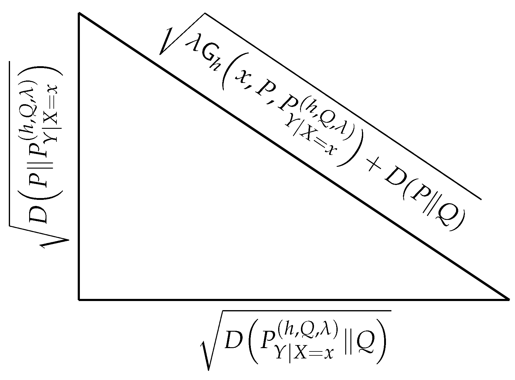
which is known as the Pythagorean theorem for relative entropy. Such a geometric interpretation follows from admitting relative entropy as an analog of squared Euclidean distance. The first appearance of such a “Pythagorean theorem” was in [12] and was later revisited in [13]. Interestingly, the same result can be obtained from Lemma 3 by noticing that for all , with in (26),
The converse of the Pythagorean theorem [41] together with Lemma 3, lead to the geometric construction shown in Figure 1. A similar interpretation was also presented in [11] and [11] in the context of the generalization error of machine learning algorithms. The former considers , while the latter considers . Nonetheless, the interpretation in Figure 1 is general and independent of such an application.
The relevance of Lemma 3, with respect to this body of literature on information projections, follows from the fact that Q might be a -finite measure, which is a class of measures that includes the class of probability measures, and thus, unifies the results separately obtained in the realm of maximum entropy methods and information-projection methods. More importantly, when , with in (26), it might hold that or , with in (18), which resonates with the fact that -Gibbs conditional probability measures are also related to another class of optimization problems, as shown by the following lemma.
Lemma 4.
Assume that the following optimization problems possess at least one solution for some ,
and
Consider the -Gibbs probability measure in (10), with such that . Then, the -Gibbs probability measure is a solution to (4) if ; or to (4) if .
Proof:
Note that if , then, . Hence, from Lemma 3, it holds that for all probability mesures P such that ,
with equality if . This implies that is a solution to (4). Note also that if , from Lemma 3, it holds that for all probability mesures P such that ,
with equality if . This implies that is a solution to (4). □
3. Characterization of in (1)
The main result of this section is the following theorem.
Theorem 1.
For all probability measures and , both absolutely continuous with respect to a given σ-finite measure Q on , the variation in (1) satisfies,
where the probability measure , with , is an -Gibbs probability measure.
Proof:
The proof follows from Lemma 3 and by observing that
□
Theorem 1 might be particularly simplified in the case in which the reference measure Q is a probability measure. Consider for instance the case in which (or ). In such a case, the reference measure might be chosen as (or ), as shown hereunder.
Corollary 1.
Consider the variation in (1). If the probability measure is absolutely continuous with respect to , then,
Alternatively, if the probability measure is absolutely continuous with respect to , then,
where the probability measures and are respectively - and -Gibbs probability measures, with .
In the case in which neither is absolutely continuous with respect to ; nor is absolutely continuous with respect to , the reference measure Q in Theorem 1 can always be chosen as a convex combination of and . That is, for all Borel sets , , with .
Theorem 1 can be specialized to the specific cases in which Q is the Lebesgue or the counting measure.
If Q is the Lebesgue measure the probability measures and in (38) admit probability density functions and , respectively. Moreover, the terms and are Shannon’s differential entropies [4] induced by and , denoted by and , respectively. That is, for all ,
The probability measure , with , , and Q the Lebesgue measure, possesses a probability density function, denoted by , which satisfies
If Q is the counting measure the probability measures and in (38) admit probability mass functions and , with a countable subset of . Moreover, and are respectively Shannon’s discrete entropies [4] induced by and , denoted by and , respectively. That is, for all ,
The probability measure , with and Q the counting measure, possesses a conditional probability mass function, denoted by , which satisfies
These observations lead to the following corollary of Theorem 1.
Corollary 2.
Given two probability measures and , with probability density functions and respectively, the variation in (1) satisfies,
4. Characterizations of in (2)
The main result of this section is a characterization of in (2).
Theorem 2.
Consider the variation in (2) and assume that for all , the probability measures and are both absolutely continuous with respect to a σ-measure Q. Then,
where the probability measure , with , is an -Gibbs conditional probability measure.
Proof:
The proof follows from (2) and Theorem 1. □
Two special cases are particularly noteworthy.
When the reference measure Q is the Lebesgue measure
When the reference measure Q is the counting measure
both and in (47) become Shannon’s discrete conditional entropies, denoted by and , respectively. That is, for all ,
where is the entropy functional in (43).
These observations lead to the following corollary of Theorem 2.
Corollary 3.
Consider the variation in (2) and assume that for all , the probability measures and possess probability density functions. Then,
Note that, from (2), it follows that the general expression for the expected variation might be simplified according to Corollary 1. For instance, if for all , the probability measure is absolutely continuous with respect to , the measure can be chosen to be the reference measure in the calculation of in (2). This observation leads to the following corollary of Theorem 2.
Corollary 4.
Alternatively, if for all , the probability measure is absolutely continuous with respect to , then,
where the measures and are respectively - and -Gibbs probability measures.
The Gibbs probability measures and in Corollary 4 are particularly interesting as their reference measures depend on x. Gibbs measures of this form appear, for instance, in [8].
5. Characterizations of in (6)
The main result of this section is a characterization of in (6), which describes the variation of the expectation of the function h when the probability measure changes from the joint probability measure to the product of its marginals . This result is presented hereunder and involves the mutual information and lautum information , defined as follows:
Theorem 3.
Consider the expected variation in (6) and assume that, for all :
- The probability measures and are both absolutely continuous with respect to a given σ-finite measure Q; and
- The probability measures and are mutually absolutely continuous.
Then, it follows that
where the probability measure , with , is an -Gibbs conditional probability measure.
Proof:
The proof is presented in Appendix A. □
An alternative expression for in (6) involving only relative entropies is presented by the following theorem.
Theorem 4.
Consider the expected variation in (6) and assume that, for all , the probability measure is absolutely continuous with respect to a given σ-finite measure Q. Then, it follows that
where , with , is an -Gibbs conditional probability measure.
Proof:
The proof is presented in Appendix B. □
Theorem 4 expresses the variation in (6) as the expectation (w.r.t. ) of a comparison of the conditional probability measure with a Gibbs conditional probability measure via relative entropy. More specifically, the expression consists in the expectation of the difference of two relative entropies. The former compares with , where are independently sampled from the same probability measure . The latter compares these two conditional measures conditioning on the same element of . That is, it compares with .
An interesting observation from Theorem 3 and Theorem 4 is that the last two terms in the right-hand side of (56) are both zero in the case in which is an -Gibbs conditional probability measure. Similarly, in such a case, the second term in the right-hand side of (57) is also zero. This observation is highlighted by the following corollary.
Corollary 5.
Consider an -Gibbs conditional probability measure, denoted by , with ; and a probability measure . Let the measure be such that for all sets ,
Then,
Note that mutual information and lautum information are both nonnegative information measures, which from Corollary 5, implies that in (59) might be either positive or negative depending exclusively on the sign of the regularization factor . The following corollary exploits such an observation to present a property of Gibbs conditional probability measures and their corresponding marginal probability measures.
Corollary 6.
Given a probability measure , the -Gibbs conditional probability measure in (10) and the probability measure in (58) satisfy
or
Corollary 6 highlights the fact that a deviation from the joint probability measure to the product of its marignals might increase or decrease the expectation of the function h depending on the sign of .
6. Final Remarks
A simple re-formulation of Varandan’s variational representation of relative entropy (Lemma 2) has been harnessed to provide an explicit expression of the variation of the expectation of a multi-dimensional real function when the probability measure changes from a Gibbs probability measure to an arbitrary measure (Lemma 3). This result reveals strong connections with information projection methods, Pythagorean identities involving relative entropy, and mean optimization problems constrained to a neighborhood around a reference measure, where the neighborhood is defined via an upper bound on relative entropy with respect to the reference measure (Lemma 4). An algebraic manipulation on Lemma 3 leads to an explicit expression for the variation of the expectation under study when the probability measure changes from an arbitrary measure to another arbitrary measure (Theorem 1). The astonishing simplicity in the proof, which is straight forward from Lemma 3, contrasts with the generality of the result. In particular, the only assumption is that both measures, before and after the variation, are absolutely continuous with a reference measure. The underlying observation is the central role played by Gibbs probability distributions in this analysis. In particular, such a variation is expressed in terms of comparisons, via relative entropy, of the initial and final probability measures with respect to the Gibbs probability measure specifically built for the function under study. Interestingly, the reference measure of such Gibbs probability measures can be freely chosen beyond probability measures. When such a reference is a -finite measure, e.g., Lebesgue measure or a counting measure, the expressions mentioned above include Shannon’s fundamental information measures, e.g., entropy and conditional entropy (Corollary 2).
Using these initial results, the variations of expectations of multi-dimensional functions due to variations of joint probability measures has been studied. In this case, the focus has been on two particular measure changes, which unveil connections with both mutual and lautum information. First, one of the marginal probability measures remains the same after the change (Theorem 2); and second, the joint probability measure changes to the product of its marginals (Theorem 3 and Theorem 4). In the case of Gibbs joint probability measures, these expressions involve exclusively well known information measures: mutual information; lautum information; and relative entropy. These expressions reveal general connections between the variation in the expectation of arbitrary functions, induced by changes in the underlying probability measure, and both mutual and lautum information. These connections extend beyond those previously established in the analysis of generalization error in machine learning algorithms; see, for instance, [26] and [8].
Author Contributions
All authors contributed equally to this research.
Funding
This research was supported in part by the European Commission through the H2020-MSCA-RISE-2019 project 872172; the French National Agency for Research (ANR) through the Project ANR-21-CE25-0013 and the project ANR-22-PEFT-0010 of the France 2030 program PEPR Réseaux du Futur; and in part with the Agence de l’innovation de défense (AID) through the project UK-FR 2024352
Conflicts of Interest
The authors declare no conflicts of interest.
Appendix A. Proof of Theorem 3
The proof follows from Theorem 2, which holds under assumption and leads to
Appendix B. Proof of Theorem 4
The proof follows by observing that the functional in (6) satisfies
References
- Gama, J.; Medas, P.; Castillo, G.; Rodrigues, P. Learning with drift detection. In Proceedings of the Proceedings of the 17th Brazilian Symposium on Artificial Intelligence, Sao Luis, Maranhao, Brazil, Oct. 2004; pp. 286–295.
- Webb, G.I.; Lee, L.K.; Goethals, B.; Petitjean, F. Analyzing concept drift and shift from sample data. Data Mining and Knowledge Discovery 2018, 32, 1179–1199. [Google Scholar] [CrossRef]
- Oliveira, G.H.F.M.; Minku, L.L.; Oliveira, A.L. Tackling virtual and real concept drifts: An adaptive Gaussian mixture model approach. IEEE Transactions on Knowledge and Data Engineering 2021, 35, 2048–2060. [Google Scholar] [CrossRef]
- Shannon, C.E. A mathematical theory of communication. The Bell System Technical Journal 1948, 27, 379–423. [Google Scholar] [CrossRef]
- Shannon, C.E. A mathematical theory of communication. The Bell System Technical Journal 1948, 27, 623–656. [Google Scholar] [CrossRef]
- Palomar, D.P.; Verdú, S. Lautum information. IEEE Transactions on Information Theory 2008, 54, 964–975. [Google Scholar] [CrossRef]
- Perlaza, S.M.; Esnaola, I.; Bisson, G.; Poor, H.V. On the Validation of Gibbs Algorithms: Training Datasets, Test Datasets and their Aggregation. In Proceedings of the Proceedings of the IEEE International Symposium on Information Theory (ISIT), Taipei, Taiwan, Jun. 2023.
- Perlaza, S.M.; Bisson, G.; Esnaola, I.; Jean-Marie, A.; Rini, S. Empirical Risk Minimization with Relative Entropy Regularization. IEEE Transactions on Information Theory 2024, 70, 5122–5161. [Google Scholar] [CrossRef]
- Zou, X.; Perlaza, S.M.; Esnaola, I.; Altman, E. Generalization Analysis of Machine Learning Algorithms via the Worst-Case Data-Generating Probability Measure. In Proceedings of the Proceedings of the AAAI Conference on Artificial Intelligence, Vancouver, Canada, Feb.
- Zou, X.; Perlaza, S.M.; Esnaola, I.; Altman, E.; Poor, H.V. The Worst-Case Data-Generating Probability Measure in Statistical Learning. IEEE Journal on Selected Areas in Information Theory 2024, 5, 175–189. [Google Scholar] [CrossRef]
- Perlaza, S.M.; Zou, X. The Generalization Error of Machine Learning Algorithms. arXiv 2024. [Google Scholar] [CrossRef]
- Chentsov, N.N. Nonsymmetrical distance between probability distributions, entropy and the theorem of Pythagoras. Mathematical notes of the Academy of Sciences of the USSR 1968, 4, 686–691. [Google Scholar] [CrossRef]
- Csiszár, I.; Matus, F. Information projections revisited. IEEE Transactions on Information Theory 2003, 49, 1474–1490. [Google Scholar] [CrossRef]
- Müller, A. Integral probability metrics and their generating classes of functions. Advances in applied probability 1997, 29, 429–443. [Google Scholar] [CrossRef]
- Zolotarev, V.M. Probability metrics. Teoriya Veroyatnostei i ee Primeneniya 1983, 28, 264–287. [Google Scholar] [CrossRef]
- Gretton, A.; Borgwardt, K.M.; Rasch, M.J.; Schölkopf, B.; Smola, A. A Kernel Two-Sample Test. Journal of Machine Learning Research 2012, 13, 723–773. [Google Scholar]
- Villani, C. Optimal transport: Old and new, first ed.; Springer: Berlin, Germany, 2009. [Google Scholar]
- Liu, W.; Yu, G.; Wang, L.; Liao, R. An Information-Theoretic Framework for Out-of-Distribution Generalization with Applications to Stochastic Gradient Langevin Dynamics. arXiv 2024, arXiv:2403.19895 2024. [Google Scholar]
- Liu, W.; Yu, G.; Wang, L.; Liao, R. An Information-Theoretic Framework for Out-of-Distribution Generalization. In Proceedings of the Proceedings of the IEEE International Symposium on Information Theory (ISIT), Athens, Greece, July 2024; pp. 2670–2675.
- Agrawal, R.; Horel, T. Optimal Bounds between f-Divergences and Integral Probability Metrics. Journal of Machine Learning Research 2021, 22, 1–59. [Google Scholar]
- Rahimian, H.; Mehrotra, S. Frameworks and results in distributionally robust optimization. Open Journal of Mathematical Optimization 2022, 3, 1–85. [Google Scholar] [CrossRef]
- Xu, C.; Lee, J.; Cheng, X.; Xie, Y. Flow-based distributionally robust optimization. IEEE Journal on Selected Areas in Information Theory 2024, 5, 62–77. [Google Scholar] [CrossRef]
- Hu, Z.; Hong, L.J. Kullback-Leibler divergence constrained distributionally robust optimization. Optimization Online 2013, 1, 9. [Google Scholar]
- Radon, J. Theorie und Anwendungen der absolut additiven Mengenfunktionen, first ed.; Hölder: Vienna, Austria, 1913. [Google Scholar]
- Nikodym, O. Sur une généralisation des intégrales de MJ Radon. Fundamenta Mathematicae 1930, 15, 131–179. [Google Scholar] [CrossRef]
- Aminian, G.; Bu, Y.; Toni, L.; Rodrigues, M.; Wornell, G. An Exact Characterization of the Generalization Error for the Gibbs Algorithm. Advances in Neural Information Processing Systems 2021, 34, 8106–8118. [Google Scholar]
- Perlaza, S.M.; Bisson, G.; Esnaola, I.; Jean-Marie, A.; Rini, S. Empirical Risk Minimization with Relative Entropy Regularization: Optimality and Sensitivity. In Proceedings of the Proceedings of the IEEE International Symposium on Information Theory (ISIT), Espoo, Finland, Jul. 2022; pp. 684–689.
- Jiang, W.; Tanner, M.A. Gibbs posterior for variable selection in high-dimensional classification and data mining. The Annals of Statistics 2008, 36, 2207–2231. [Google Scholar] [CrossRef]
- Perlaza, S.M.; Esnaola, I.; Bisson, G.; Poor, H.V. On the Validation of Gibbs Algorithms: Training Datasets, Test Datasets and their Aggregation. In Proceedings of the Proceedings of the IEEE International Symposium on Information Theory (ISIT), Taipei, Taiwan, Jun. 2023.
- Alquier, P.; Ridgway, J.; Chopin, N. On the properties of variational approximations of Gibbs posteriors. Journal of Machine Learning Research 2016, 17, 8374–8414. [Google Scholar]
- Bu, Y.; Aminian, G.; Toni, L.; Wornell, G.W.; Rodrigues, M. Characterizing and understanding the generalization error of transfer learning with Gibbs algorithm. In Proceedings of the Proceedings of the 25th International Conference on Artificial Intelligence and Statistics (AISTATS), Virtual Conference, Mar. 2022; pp. 8673–8699.
- Raginsky, M.; Rakhlin, A.; Tsao, M.; Wu, Y.; Xu, A. Information-theoretic analysis of stability and bias of learning algorithms. In Proceedings of the Proceedings of the IEEE Information Theory Workshop (ITW), Cambridge, UK, Sep. 2016; pp. 26–30.
- Zou, B.; Li, L.; Xu, Z. The Generalization Performance of ERM algorithm with Strongly Mixing Observations. Machine Learning 2009, 75, 275–295. [Google Scholar] [CrossRef]
- He, H.; Aminian, G.; Bu, Y.; Rodrigues, M.; Tan, V.Y. How Does Pseudo-Labeling Affect the Generalization Error of the Semi-Supervised Gibbs Algorithm? In Proceedings of the Proceedings of the 26th International Conference on Artificial Intelligence and Statistics (AISTATS), Valencia, Spain, Apr. 2023; pp. 8494–8520. [Google Scholar]
- Hellström, F.; Durisi, G.; Guedj, B.; Raginsky, M. Generalization Bounds: Perspectives from Information Theory and PAC-Bayes. Foundations and Trends® in Machine Learning 2025, 18, 1–223. [Google Scholar] [CrossRef]
- Jaynes, E.T. Information Theory and Statistical Mechanics I. Physical Review Journals 1957, 106, 620–630. [Google Scholar] [CrossRef]
- Jaynes, E.T. Information Theory and Statistical Mechanics II. Physical Review Journals 1957, 108, 171–190. [Google Scholar] [CrossRef]
- Kapur, J.N. Maximum Entropy Models in Science and Engineering, first ed.; Wiley: New York, NY, USA, 1989. [Google Scholar]
- Bermudez, Y.; Bisson, G.; Esnaola, I.; Perlaza, S.M. Proofs for Folklore Theorems on the Radon-Nikodym Derivative. Technical Report RR-9591, INRIA, Centre Inria d’Université Côte d’Azur, Sophia Antipolis, France, 2025.
- Donsker, M.D.; Varadhan, S.S. Asymptotic evaluation of certain Markov process expectations for large time, I. Communications on pure and applied mathematics 1975, 28, 1–47. [Google Scholar] [CrossRef]
- Heath, T.L. The Thirteen Books of Euclid’s Elements, 2nd revised edition ed.; Dover Publications, Inc.: New York, 1956. [Google Scholar]
Figure 1.
Geometric interpretation of Lemma 3, with Q a probability measure.
Disclaimer/Publisher’s Note: The statements, opinions and data contained in all publications are solely those of the individual author(s) and contributor(s) and not of MDPI and/or the editor(s). MDPI and/or the editor(s) disclaim responsibility for any injury to people or property resulting from any ideas, methods, instructions or products referred to in the content. |
© 2025 by the authors. Licensee MDPI, Basel, Switzerland. This article is an open access article distributed under the terms and conditions of the Creative Commons Attribution (CC BY) license (http://creativecommons.org/licenses/by/4.0/).
Copyright: This open access article is published under a Creative Commons CC BY 4.0 license, which permit the free download, distribution, and reuse, provided that the author and preprint are cited in any reuse.


