
Submitted:
24 July 2025
Posted:
24 July 2025
You are already at the latest version
Abstract
In recent years, deep learning has become a dominant research trend in the field of remote sensing. However, due to significant domain discrepancies among datasets collected from various platforms, models trained on a single domain often struggle to generalize to other domains. In domain-incremental learning scenarios, such discrepancies often lead to catastrophic forgetting, hindering the practical deployment of deep learning models. To address this challenge, we propose ER-PASS, an experience replay-based continual learning algorithm that incorporates a performance-aware submodular sampling strategy. ER-PASS effectively balances adaptability across domains and retention of knowledge by integrating the strengths of joint learning and experience replay, while maintaining practical efficiency in terms of training time and memory usage. Additionally, by leveraging a performance-aware sample selection strategy that integrates submodular gain and task-specific evaluation scores, ER-PASS enables robust and stable learning. Experimental results on two distinct applications—building segmentation and land use/land cover (LULC) classification—demonstrate that ER-PASS outperforms existing continual learning methods in mitigating forgetting and generalizing across diverse application scenarios. Moreover, experiments conducted on both UNet and DeepLabV3+ validate the model-agnostic nature of ER-PASS, underscoring its potential as a practical and general-purpose solution for continual learning in remote sensing.
Keywords:
remote sensing
; deep learning
; continual learning
; domain-incremental learning
; experience replay
; catastrophic forgetting
1. Introduction
Recent advances in remote sensing technologies have enabled the acquisition of large volumes of imagery from diverse platforms, including satellites, drones, and airborne systems. This has led to the extensive application of remote sensing data in various fields such as urban planning [1,2,3,4], environmental monitoring [5,6,7], and disaster management [8,9,10]. Furthermore, the introduction of deep learning techniques has significantly enhanced the efficiency and accuracy of remote sensing image analysis, achieving state-of-the-art performance across a wide range of applications [11,12,13,14,15]. For instance, tasks such as building segmentation and land use/land cover (LULC) classification, which previously relied on manual interpretation or basic analytical methods, have seen remarkable improvements in both accuracy and computational efficiency through the application of deep learning [16,17,18]. Consequently, the research paradigm in remote sensing has shifted from traditional rule-based approaches to data-driven, deep learning-based methods.
Most deep learning studies in remote sensing have focused on improving task performance using fixed datasets under static experimental settings, with the development of state-of-the-art models becoming a dominant research trend. However, in real-world scenarios, imagery is continuously collected from various platforms, leading to significant variations in visual characteristics—such as object size, shape, and texture—as illustrated in Figure 1. Due to these domain-specific discrepancies, models trained on a single domain (i.e., a set of images from a specific platform) often suffer from severe performance degradation when applied to new domains [19,20]. This necessitates retraining the model for each new domain, which is not only computationally expensive but also risks catastrophic forgetting [21,22], where previously learned knowledge is lost during adaptation. These limitations hinder the practical deployment of deep learning-based remote sensing methods and highlight the need for more flexible and adaptive learning strategies. In this context, continual learning has emerged as a promising approach capable of mitigating both domain shift problems and catastrophic forgetting.
Continual learning is a learning paradigm in which a model incrementally learns from a sequence of tasks, aiming to integrate new knowledge without forgetting what has already been learned [23,24]. In this context, a "task" refers to a specific learning objective that arises sequentially over time. Based on learning scenarios, continual learning is typically categorized into Task-Incremental Learning (TIL), Class-Incremental Learning (CIL), and Domain-Incremental Learning (DIL) [25,26]. In TIL, each task has a distinct label space, and a task identifier is available during both the training and inference to specify which task the model should address. In contrast, CIL does not provide a task identifier during inference, requiring the model to classify all previously encountered classes jointly. DIL differs from the previous two scenarios by maintaining a shared label space across tasks, while varying the input distribution or domain characteristics. Among the three, DIL is particularly relevant to real-world remote sensing applications, where domain shifts frequently occur. Nevertheless, research on DIL remains relatively underexplored compared to the TIL and CIL. Therefore, this study focuses on addressing challenges within the DIL scenario.
In addition to scenario-based categorization, continual learning can also be classified based on implementation strategies: regularization-based, architecture-based, and replay-based methods [27,28]. Regularization-based methods preserve prior knowledge by incorporating additional terms into the loss function that penalize changes to parameters important for previous tasks. Architecture-based methods maintain prior knowledge by isolating parameters for each task, either by fixing and masking them during the training of new tasks or by using dynamic architectures that freeze existing parameters while expanding the model for task-specific learning. Replay-based methods, on the other hand, preserve prior knowledge more intuitively by explicitly storing a subset of data from previous tasks in a memory buffer and reusing it when training on new tasks.
Most existing studies on DIL have primarily employed regularization-based or architecture-based approaches, often citing concerns regarding data storage costs and privacy issues associated with replay-based methods [29,30,31]. However, in the field of remote sensing, long-term data collection is standard practice, making data storage costs a less critical concern. Furthermore, remote sensing imagery typically does not contain personally identifiable information, reducing privacy risks compared to other fields—except in sensitive areas such as national defense. Instead, the limitations of regularization-based and architecture-based methods pose significant challenges in practical remote sensing applications. Regularization-based methods are inherently vulnerable to domain shifts, which can lead to catastrophic forgetting. Meanwhile, architecture-based methods tend to increase model complexity as tasks accumulate, requiring additional memory resources. Given these factors, replay-based methods present a more practical solution for DIL within remote sensing.
Therefore, this study aims to develop a replay-based learning algorithm tailored for remote sensing in DIL scenarios. Specifically, we propose an experience replay with performance-aware submodular sampling (ER-PASS). ER-PASS is designed to improve the adaptability of deep learning models across remote sensing domains, while mitigating catastrophic forgetting and ensuring computational efficiency. To this end, ER-PASS integrates the robustness of joint learning—by processing samples from multiple domains as a unified input—with the efficiency of replay-based learning in reducing training time. Additionally, we introduce a performance-aware submodular sample selection strategy to enhance the stability of the learning process. To evaluate the generalizability of our approach, we conduct extensive experiments on two representative remote sensing applications: building segmentation and LULC classification. The main contributions of this study are as follows:
- (1)
- We propose a replay-based learning algorithm that incorporates a performance-aware submodular sample selection strategy, namely ER-PASS, which is model-agnostic and can be applied across various deep learning models.
- (2)
- We demonstrate that ER-PASS effectively mitigates catastrophic forgetting compared to existing methods, while requiring relatively low resource demands.
- (3)
- Experimental results on building segmentation and LULC classification demonstrate that ER-PASS exhibits generalizability across diverse remote sensing applications.
2. Related Work
2.1. Domain-Incremental Learning in Remote Sensing
Recently, continual learning has received increasing attention in the field of remote sensing. However, most existing studies have primarily focused on TIL or CIL [32,33,34,35,36], while research on DIL remains limited. To address this gap, several recent works have begun investigating DIL in remote sensing contexts. Marsocci and Scardapane [37] were the first to explore semantic segmentation of remote sensing imagery in the context of DIL, proposing a loss function that combines Elastic Weight Consolidation (EWC) [38] and Barlow Twins [39] to simultaneously address label scarcity and catastrophic forgetting. Rui et al. [29] introduced the DILRS architecture, which employs a shared encoder and domain-specific decoders to capture both domain-invariant and domain-specific features. They addressed label space shifts across domains by applying a multi-level class-specific knowledge distillation loss. Wang et al. [30] developed a self-knowledge distillation model that incorporates dynamic equilibrium constraints and learnable loss weights, effectively closing the performance gap with joint training in cross-domain fire detection. Additionally, Huang et al. [31] proposed a DIL framework leveraging frozen feature layers and a multi-feature joint loss to alleviate catastrophic forgetting. Although these studies offer valuable contributions, most rely predominantly on regularization-based or architecture-based approaches. Given the characteristics of remote sensing imagery, the use of replay-based methods, though less explored, hold significant promise, as discussed in the following section.
2.2. Replay-Based Continual Learning Algorithms
The core challenges of continual learning stem from the need to balance knowledge transfer and interference between tasks. This balance is closely related to the angles between the gradients of the loss functions for different tasks during stochastic gradient descent [40]. Specifically, learning interference occurs when the angle between these gradients exceeds 90 degrees, hindering knowledge transfer. Motivated by this insight, replay-based continual learning methods seek to reduce interference by controlling or projecting gradients to keep their angles below this threshold. For instance, Lopez-Paz and Ranzato [41] proposed Gradient Episodic Memory (GEM), which compares the current task’s gradient with those of previous tasks stored in a memory buffer and projects the current gradient to ensure the angle with previous task gradients does not exceed 90 degrees, thereby preventing interference. To improve computational efficiency, Chaudhry et al. [42] introduced Averaged GEM (A-GEM), which replaces task-specific gradient comparisons with a single comparison against the average gradient computed from the memory buffer, avoiding per-task gradient computations. Alternatively, Experience Replay (ER) [43] adopts a different approach by directly reusing stored samples instead of manipulating gradients. ER jointly samples mini-batches from the current task and the memory buffer for optimization, avoiding explicit gradient projection while still effectively mitigating catastrophic forgetting. Building on this approach, several replay-based continual learning methods have been developed in the computer vision community, including MER, DER and iCaRL [44,45,46].
Despite their success in computer vision, replay-based methods have seen limited application in remote sensing. Among the few studies, Bhat et al. [47] proposed a curriculum-based memory replay strategy to improve scene classification in remote sensing imagery. Sun et al. [48] evaluated various continual learning methods and highlighted that combining replay of representative samples with knowledge distillation enhances synthetic aperture radar (SAR)-based automatic target recognition accuracy. These early efforts demonstrate the potential of replay-based methods in remote sensing. However, they mainly focus on CIL rather than DIL, which is a common in real-world scenarios. To fill this gap, we propose an effective replay-based learning algorithm tailored for DIL.
2.3. Sample Selection Strategies for Replay
Sample selection, also called coreset selection, plays a crucial role in replay-based continual learning by efficiently managing the memory buffer, directly impacting both model performance and memory utilization. Early studies often employed simple strategies such as reservoir sampling [49] and ring buffers [41], which generally preserve data diversity but do not explicitly consider the importance of individual samples. Subsequent methods, including k-Center Greedy [50] and Mean of Features (MoF) [46] aim to select representative samples in the feature space, thereby improving representativeness. However, these methods may neglect rare or boundary samples that are crucial for robust generalization.
Recent submodular-based sample selection methods have gained attention. For instance, Yoon et al. [51] proposed a method that considers intra-batch similarity, sample diversity, and affinity to past tasks, thereby enhancing model adaptation while reducing catastrophic forgetting. Similarly, Lee et al. [52] addressed the object detection by generating representative feature vectors for multiple objects of the same class within each image and applying submodular-based greedy selection, showing better performance that random sampling. While these approaches provide a solid framework for capturing sample diversity and coverage, they do not explicitly account for the each sample’s influence on model optimization.
On the other hand, gradient-based methods emphasize the impact of individual samples on model optimization. Notably, Aljundi et al. [53] formulated sample selection as a constraint reduction problem, selecting coreset examples whose aggregated gradients closely approximate the average gradient of the full dataset. This approach helps maintain stable optimization during continual learning. However, by focusing on average gradient preservation, it may dilute the influence of critical samples near decision boundaries that are crucial for model performance. To overcome this limitation, we propose a performance-aware submodular sample selection strategy that incorporates model predictions into the selection criteria. This enables the memory buffer to retain samples that are not only representative and diverse, but also particularly informative for refining decision boundaries, thereby enhancing the stability of the continual learning process.
3. Methodology
3.1. Overview
This study is conducted under the DIL scenario, where data from multiple platforms are incrementally collected, and the model is continuously updated to accommodate newly acquired data. In this setting, learning for each domain is treated as an individual task, and the number of tasks increases as new domain data becomes available. A strict DIL setup assumes that class labels remain consistent across tasks. To align with this assumption, we adopt building segmentation as the primary downstream application. However, real-world scenarios often involve the emergence of new classes over time. To reflect such practical considerations, we additionally evaluate our approach under a more relaxed setting using LULC classification, where new classes can emerge in later tasks.
The overall learning process of ER-PASS proposed in this study is illustrated in Figure 2. For each domain, the segmentation model is trained sequentially, followed by a sample selection step that stores representative samples in the memory buffer. This buffer helps retain knowledge from previous domains and supports learning in future domains. During evaluation, the model is assessed not only on the current domain but also on all previously encountered domains. We adopt UNet [54] and DeepLabV3+ [55] as baseline models for both the building segmentation and LULC classification. Notably, ER-PASS is model-agnostic and can be readily integrated into other segmentation networks without requiring any architectural modifications.
3.2. Proposed Algorithm
ER-PASS is a replay-based continual learning algorithm tailored for DIL in remote sensing applications. It is motivated by the observation that joint learning has been shown to improve generalization across heterogeneous domains and that dataset-level memory integration—rather than batch-level—offers greater computational efficiency.
Let the continual learning process consist of a sequence of tasks , each corresponding to a distinct remote sensing domain. For the k-th task , a labeled dataset is provided, where and denote the input image and its corresponding label, and is the number of training samples in task .
Unlike conventional experience replay methods [43,44,45], which merge current task data and memory buffer samples within each mini-batch, ER-PASS performs dataset-level integration by combining the two into a unified training set. Specifically, for task , the new training set is defined as:
where denotes the memory buffer containing representative samples from previous tasks. The model parameters for task are then optimized by minimizing the expected loss over the combined dataset :
where denotes the downstream segmentation loss (e.g., binary cross-entropy or cross-entropy), and represents the segmentation model.
Through this simple yet effective approach, ER-PASS computes a single gradient per iteration without requiring gradient aggregation, while maintaining a consistent batch size. This design reduces memory overhead compared to conventional replay-based methods and shortens training time compared to joint learning by relying only on a compact memory buffer rather than the full dataset of previous tasks.
After training on task , a sample selection algorithm is employed to extract a representative subset of samples from for updating the memory buffer. The selection is based on feature similarity and task-specific performance, as described in Section 3.3:
The updated memory is then used for training on the next task . The overall learning process of ER-PASS is summarized in Algorithm 1.
| Algorithm 1 Learning process of ER-PASS |
|
Input:▹ Dataset corresponding to each task
Require:▹ Neural network
Initialize:▹ Memory buffer Define as the training set used for task k
for task do
if t = 1 then
▹ Initialize model parameters else
end if
Define as the total number of mini-batches in
for do
▹ Update model end for
▹ Update memory buffer end for |
3.3. Performance-Aware Submodular Sample Selection
In ER-PASS, the samples stored in the memory buffer from previous tasks are essential to preserving knowledge. To ensure effective knowledge retention, we propose a performance-aware submodular sample selection strategy that jointly considers both feature-level diversity and task-specific prediction performance. This strategy promotes the retention of diverse, representative, and informative samples, thereby improving stability and mitigating catastrophic forgetting during learning process.
For each candidate sample , we extract the feature representation by applying global average pooling to the encoder output of the trained model . Here, d denotes the dimensionality of the features space, which corresponds to 512 for UNet and 2048 for DeepLabV3+. Specifically, we use the output of the final downsampling block in the UNet encoder and the output of layer4 in the ResNet50 backbone of DeepLabV3+ as the feature map. Each feature vector is then -normalized to ensure consistent scaling, using the following equation:
We also compute a task-specific evaluation score , such as the Intersection-over-Union (IoU) or mean Intersection-over-Union (mIoU) between the model’s prediction and the ground truth. This score serves as a performance-based weight during sample selection.
Let denote the set of normalized feature vectors extracted from all candidate samples. The intra-similarity of a candidate sample is defined as the total cosine similarity between its feature vector and those of all other vectors in :
This term reflects the alignment of with the candidate sample distribution in the feature space, promoting the selection of representative and diverse samples.
Let be the set of feature vectors corresponding to the samples already selected into the memory buffer. The inter-similarity of with respect to is then defined as:
This measures the redundancy of relative to the selected set. A lower inter-similarity indicates that the sample introduces novel information, contributing to buffer diversity.
We define the selection scores for each candidate as the submodular gain—the difference between intra- and inter-similarity—weighted by task-specific evaluation score:
At each iteration, the candidate with the highest score is greedily selected and added to the memory buffer:
This process continues until a predefined budget—such as a fixed number of samples or percentage of the dataset—is reached. By jointly optimizing representativeness (via intra-similarity), redundancy reduction (via inter-similarity), and task relevance (via evaluation score), the proposed strategy constructs a memory buffer that is both submodular-optimal and performance-sensitive, effectively supporting continual learning. The detailed procedure is described in Algorithm 2.
| Algorithm 2 Performance-aware submodular sample selection |
|
Input:, ▹ Dataset and trained model corresponding to
Require:N▹ Memory budget (number of samples to select)
Output:▹ Updated memory buffer Initialize , ,
Extract features from for each sample
Compute normalized features:
Compute evaluation score between and ground truth for each sample Let , where n is the total number of samples in
Compute intra-similarity:
for to N do
for to n do
if then
▹ Only intra-similarity else
Compute inter-similarity:
end if
if ▹ Exclude already selected samples end for
, ,
end for |
4. Experimental Settings
4.1. Datasets
In this study, we designed a domain sequence to reflect practical scenarios that may arise when utilizing remote sensing imagery. The construction was guided by the following three criteria: (1) each dataset should be acquired from a distinct sensing platform; (2) data within each dataset should originate from a single, consistent platform; and (3) the datasets should vary in spatial resolution. Based on these criteria, we selected four representative LULC datasets—Potsdam [56], LoveDA [57], DeepGlobe [58], and GID [59]—each representing a distinct domain ( to ).
Details of the constructed domain sequence are summarized in Table 1. Depending on the dataset, data were either provided as training-only or with a predefined training/test split. For training-only datasets, we divided the data into training, validation, and test sets using an 4:1:1 ratio. For datasets with a predefined split, the training portion was further divided into training and validation subsets in an 8:2 ratio, while the provided test set was retained for evaluation. To ensure a comparable number of training samples across domains, all images were divided into patches using dataset-specific stride values. Additionally, since the class definitions and label structures differ across datasets, we grouped semantically similar classes into unified categories. We first conducted binary segmentation experiments focusing exclusively on the building class, where building pixels were labeled as 1 and all other as 0. Subsequently, we extended the experiments to multi-class LULC classification using the redefined label categories for each dataset.
4.2. Implementation Details
We selected building segmentation and LULC classification as the downstream applications and conducted incremental learning experiments for each. To demonstrate the model-agnostic nature of ER-PASS, we utilized UNet [54] and DeepLabV3+ [55] as base models for both applications. As the primary focus of this study is on learning strategy rather than architectural design, no modifications were made to the base network architectures. For building segmentation, we employed binary cross-entropy loss, while multi-class cross-entropy loss, based on the redefined class labels for each dataset, was used for LULC classification.
For benchmarking, ER-PASS was compared against representative continual learning methods, including EWC [38], Learning without Forgetting (LwF) [60], and ER [43]. The EWC and LwF methods incorporated regularization terms, with set to 10 and 2, respectively. For ER and the proposed ER-PASS, a memory sampling ratio of 0.5 was applied.
In the incremental learning setup, the model was randomly initialized without pretrained weights for the first task. For for subsequent tasks, the model was initialized using the weights learned from previous ones to promote knowledge transfer. Training was conducted using the NAdam optimizer with a learning rate of 0.0002 and a batch size of 8. Each experiment was run for a maximum of 100 epochs, with early stopping applied if validation performance did not improve for 10 consecutive epochs. The model achieving the best validation performance was selected for final evaluation. All experiments were implemented using PyTorch 1.12.0 and performed on a workstation equipped with 64 GB RAM and on NVIDIA RTX A6000 GPU.
4.3. Evaluation Metrics
Continual learning performance should be evaluated in terms of two key aspects: the effectiveness in learning new tasks and the capacity to mitigate forgetting of prior knowledge. To quantify these aspects, we adopt Average Incremental Accuracy (AIA) [46] and Backward Transfer (BWT) [41], defined as follows:
here, denotes the performance on the test set of the j-th task after training incrementally up to the k-th task, where .
AIA measures the overall performance of a model throughout the entire learning process. By averaging performance on each previously encountered task at every step, it captures the model’s ability to learn new tasks while retaining knowledge from earlier ones. Meanwhile, BWT quantifies the degree of knowledge retention by comparing the performance on earlier tasks before and after subsequent learning, thus serving as a direct indicator of catastrophic forgetting. As continual learning aims to balance learning new tasks and retaining prior knowledge, it is essential to consider both metrics for a comprehensive evaluation.
5. Experimental Results and Discussion
5.1. Building Segmentation (Strict DIL Setting)
As previously described, our incremental learning setup employs a step-wise training procedure across four domains in the following order: Potsdam, LoveDA, DeepGlobe and GID. The model is initially trained on Potsdam in Step 1 with randomly initialized weights. In Steps 2 to 4, the model is incrementally updated by leveraging the weights learned from the previous step, thereby facilitating knowledge transfer across domains. Under this setup, we conducted downstream evaluation on building segmentation. Experiments were primarily conducted using UNet, with additional comparisons performed using DeepLabV3+.
Table 2 presents the IoU performance at each incremental step using UNet for building segmentation, along with evaluation metrics at Step 4. At each step, the reported IoU values reflect the model’s performance on all previously encountered domains, evaluated using the model trained on the current task. Models trained via single-task learning lack adaptability to unseen domains and demonstrate satisfactory performance only within the domain on which they were trained. This limitation becomes particularly evident at Step 4, where performance on other domains significantly degrades—primarily caused by substantial domain shifts. While fine-tuning facilitates some knowledge transfer, its performance gains on previous tasks over single-task learning remain marginal, suggesting the occurrence of catastrophic forgetting. Notably, even continual learning methods such as EWC and LwF fail to provide meaningful improvements, yielding results comparable to naive fine-tuning and demonstrating limited ability to mitigate forgetting. In contrast, ER demonstrates better performance in terms of BWT, suggesting a stronger capability to retain prior knowledge. It also achieves higher AIA values compared to other baseline methods. However, comparison with single-task learning reveals that ER exhibits lower performance on the current task at each step, indicating that the high AIA is primarily due to the preservation of previous knowledge rather than effective learning of new tasks.
In theory, joint learning serves as the performance upper bound for incremental learning approaches. Our experimental results demonstrate that the proposed method achieves performance comparable to joint learning, and in some cases, even surpasses it. Furthermore, our method consistently outperforms baseline methods. These results indicate that our method not only mitigates catastrophic forgetting effectively but also maintains reasonable adaptability to new tasks. A similar trend is observed in Table 3, where DeepLabV3+ is used as the segmentation model instead of UNet. This consistent improvement across different architectures highlights that the effectiveness of the proposed algorithm is not limited to a specific model, demonstrating its model-agnostic nature.
To complement the quantitative results, Figure 3 and Figure 4 provide qualitative visualizations that further demonstrate the effectiveness of the proposed method. Figure 3 shows segmentation results from each domain using the UNet model trained up to Step 4, illustrating representative samples across domains. As expected, the segmentation performance on GID is relatively accurate since the model was directly trained on that domain. However, all benchmark methods exhibit noticeable degradation on previously learned domains. In particular, EWC and LwF fail to produce meaningful predictions, indicating that severe catastrophic forgetting has occurred. In contrast, ER performs better than these methods and partially mitigates forgetting. The proposed method maintains segmentation performance on previous domains at a level comparable to joint learning, clearly demonstrating its effectiveness in mitigating catastrophic forgetting.
Beyond the cross-domain comparison at Step 4, Figure 4 presents the step-by-step segmentation results for the first domain, analyzing how each method retains prior knowledge throughout the incremental learning process. In the case of EWC and LwF, prior knowledge is relatively well preserved up to Step 2. However, noticeable forgetting begins at Step 3, and severe catastrophic forgetting becomes evident by Step 4. ER maintains acceptable performance through Step 3, with slight degradation observed at Step 4. Consistent with earlier findings, the proposed method maintains stable performance across all steps, further demonstrating its robustness against catastrophic forgetting.
5.2. LULC Classification (Relaxed DIL Setting)
To further evaluate the generalizability of the proposed method in practical applications, we conduct experiments on LULC classification. Unlike building segmentation, which follows a strict DIL setting with consistent class labels, LULC classification represents a more relaxed and realistic scenario where new classes may emerge over time.
Table 4 and Table 5 present LULC classification results for UNet and DeepLabV3+, respectively. Similar to the building segmentation experiments, these tables provide step-wise mIoU scores and final-step metrics, with overall trends following a comparable pattern. Nonetheless, several noteworthy differences can be observed. In earlier experiments, EWC and LwF failed to retain prior knowledge, yielding near-zero scores at Step 4. In contrast, these methods exhibit relatively better performance in the LULC classification. This may be attributed to greater semantic consistency or overlap among LULC classes across domains, potentially facilitating improved knowledge retention.
Another interesting observation concerns the behavior of ER. While ER exhibited substantial forgetting at Step 4 in building segmentation, its performance degradation in LULC occurs earlier, at Step 2, and remains relatively stable in subsequent steps. This indicates that the dynamics of forgetting and retention can vary depending on the complexity and structure of the target application. Meanwhile, the proposed method consistently mitigates forgetting, as also observed in the building segmentation experiments.
Figure 5 illustrates the LULC classification results obtained with the UNet model trained up to Step 4. The results for EWC and LwF on previous domains show that predictions are primarily focused on classes such as forest, grassland, water, and agriculture, which correspond to the classes present in the GID. However, both methods largely fail to predict classes absent from GID, such as cars, roads, and barren areas, suggesting substantial forgetting of these classes. Notably, despite the building class being commonly present across all domains, both EWC and LwF still perform poorly on this class. This is likely due to substantial domain discrepancies, which hinder consistent recognition. In contrast, ER seems to retain partial retention of classes absent from GID, demonstrating better knowledge preservation across diverse classes and domains.
Figure 6 provides a detailed visualization of the forgetting dynamics across incremental steps. As confirmed by the quantitative results, substantial forgetting occurs at Step 4 in the building segmentation, whereas in the LULC classification, it emerges earlier, starting from Step 2. Specifically, in the case of ER, prediction performance on the grassland class noticeably degrades at Step 2, which corresponds to the second domain, LoveDA, where this class is absent. This implies that classes not present in the current task are more susceptible to forgetting. Similarly, at Step 3, performance on the road class deteriorates, consistent with its absence in the DeepGlobe, and this trend continues through Step 4. Notably, at Step 4, a performance degradation is also observed for the building class, which is present in the GID, aligning with earlier observations in the building segmentation experiments. In contrast, the proposed method effectively preserves a broader range of class representations across incremental steps, mitigating forgetting not only for classes currently being learned but also for those learned in previous steps. These findings suggest that the proposed method generalizes well beyond binary segmentation to more general semantic segmentation problems such as LULC classification, underscoring its robustness and scalability under both strict and relaxed DIL settings.
5.3. Ablation and Efficiency Analysis
5.3.1. Ablation Study on Proposed Sample Selection Strategy
As described earlier, the proposed sample selection strategy prioritizes samples based on a score function. This score is defined as the product of two components: the submodular gain, which promotes sample diversity and representativeness, and a task-specific evaluation score, which reflects the importance of each sample for the current task. To assess the individual contribution of each component, we conduct an ablation study using our primary experimental setup of incremental building segmentation with UNet.
Table 6 presents the results of the ablation study. Using only the submodular gain results in performance lower than the random baseline, suggesting that diversity alone may not be sufficient for effective sample selection. In contrast, using only the evaluation score yields improved performance over random selection, confirming the usefulness of task-specific information. Nevertheless, the improvement remains limited. The best performance is achieved when both components are combined, indicating that they complement each other. This demonstrates that by jointly considering both sample diversity and informativeness, the proposed sample selection method enhances robustness and overall performance throughout the learning process.
5.3.2. Effect of Sampling Ratio
In replay-based continual learning methods, the size of memory buffer—i.e., the number of stored samples—is a key factor in balancing performance and resource efficiency. Too few samples can lead to severe forgetting, while too many increase resource consumption and reduce practicality. Therefore, selecting an appropriate sampling ratio is essential for scalability in real-world applications. To better understand the impact of the sampling ratio on knowledge retention, we conducted experiments with varying ratios (0.1 to 0.9) using UNet for incremental building segmentation. For each sampling ratio, the BWT values were measured across three incremental steps (BWT2, BWT3, and BWT4), and the results are visualized in Figure 7.
As can be seen in Figure 7, increasing the sampling ratio generally led to BWT values approaching zero across all steps. In the low sampling range (0.1 to 0.4), BWT2 maintained relatively higher values, suggesting better knowledge retention in earlier stages. In contrast, BWT3 and BWT4 exhibited significantly lower values in the same range, reflecting more severe forgetting as the learning progressed. Interestingly, both BWT3 and BWT4 showed a sharp recovery at a sampling ratio of 0.5, with BWT values rapidly approached zero. Beyond this point, the BWT values remained relatively stable, with only marginal improvements, suggesting that the benefit of additional sample storage diminishes after a certain threshold. These findings indicate that, while increasing the sampling ratio is effective for reducing forgetting, storing excessive samples may not yield further performance gains and could instead introduce inefficiencies in resource usage. Therefore, we recommend using at least a 0.5 sampling ratio to ensure a desirable trade-off between performance and computational efficiency.
5.3.3. Computational Efficiency Analysis
In practical scenarios, training time and memory usage are also critical considerations for the deployment of continual learning systems. To assess these aspects, training time and memory consumption were monitored throughout our primary experimental setting. Training time was measured as the average duration per epoch during Step 4, and memory usage was recorded as the peak memory consumption observed throughout the training up to Step 4.
As shown in Table 7, joint learning took 902.55 seconds per epoch, while the proposed method only took 441.28 seconds, yielding a total reduction of about 13 hours over 100 epochs. As the number of tasks increases in future scenarios, this time gap is expected to grow even larger. This demonstrates that the proposed method offers a time-efficient solution for DIL, which is particularly beneficial in real-world applications with limited computational resources. Furthermore, the proposed algorithm demonstrated the lowest memory consumption among the continual learning benchmarks, reducing memory usage by almost half compared to ER. Although its training time is slightly longer than that of other continual learning methods, it provides a well-balanced trade-off between performance, training time, and memory efficiency. Therefore, the proposed method can be regarded as a practical and scalable solution for deploying deep learning models in remote sensing applications within DIL scenarios.
6. Conclusions
In this paper, we propose ER-PASS, an experience replay-based continual learning algorithm that leverages the strengths of joint learning and experience replay for DIL in remote sensing. ER-PASS integrates a performance-aware submodular sample selection strategy to enhance the stability of the learning process across evolving domains. We conducted experiments on two distinct remote sensing applications: building segmentation and LULC classification. The results demonstrate that ER-PASS effectively mitigates catastrophic forgetting in both cases, confirming its generalizability across diverse applications. Furthermore, experiments with multiple model architectures, including UNet and DeepLabV3+, show that ER-PASS is model-agnostic and can be flexibly integrated into various network structures. Additional analyses confirm that the proposed sample selection strategy positively impacts adaptability and forgetting mitigation, with stable performance maintained when the sampling ratio is 0.5 or higher. Finally, ER-PASS exhibits reasonable efficiency in terms of training time and memory consumption. These results suggest that ER-PASS can be practically applied in real-world remote sensing scenarios.
Nevertheless, ER-PASS has several limitations. First, this study focuses solely on optical imagery, and its generalizability to more heterogeneous remote sensing domains such as hyperspectral imagery or SAR remains to be validated in future work. Second, ER-PASS was evaluated on only two representative applications, and its applicability to a wider range of remote sensing applications, such as change detection or super-resolution, warrants further exploration. Lastly, ER-PASS, as a learning algorithm that is not dependent on specific model architectures, was validated using commonly adopted models such as UNet and DeepLabV3+. Given that most recent studies have proposed architecture-based methods, it is believed that further research is needed to compare and potentially integrate ER-PASS with these approaches.
Author Contributions
Conceptualization, Y.L.; methodology, Y.L. and D.L.; software, Y.L.; validation, Y.L.; formal analysis, Y.L., D.L. and T.K.; investigation, Y.L. and T.K.; resources, Y.K.; data curation, Y.L.; writing—original draft, Y.L.; writing—review and editing, D.L., T.K. and Y.K.; visualization, Y.L.; supervision, Y.K.; project administration, Y.K.; funding acquisition, Y.K. All authors have read and agreed to the published version of the manuscript.
Funding
This work was supported by the National Research Foundation of Korea (NRF) grant funded by the Korea government (MSIT) (NRF-2023R1A2C2005548). This work was also supported by the Korea Agency for Infrastructure Technology Advancement(KAIA) grant funded by the Ministry of Land,Infrastructure and Transport (Grant RS-2022-00155763).
Institutional Review Board Statement
Not applicable
Informed Consent Statement
Not applicable
Data Availability Statement
Publicly available datasets used in this paper are open-sourced and can be accessed through the following URLs: Potsdam: https://www.kaggle.com/datasets/bkfateam/potsdamvaihingen/ (accessed on 22 July 2025); LoveDA: https://zenodo.org/records/5706578 (accessed on 22 July 2025); DeepGlobe: https://www.kaggle.com/datasets/balraj98/deepglobe-land-cover-classification-dataset/ (accessed on 22 July 2025); GID: https://x-ytong.github.io/project/GID.html (accessed on 22 July 2025).
Acknowledgments
The Institute of Engineering Research at Seoul National University provided research facilities for this work.
Conflicts of Interest
The authors declare no conflicts of interest.
Abbreviations
The following abbreviations are used in this manuscript:
| A-GEM | Averaged GEM |
| AIA | Average Incremental Accuracy |
| BWT | Backward Transfer |
| CIL | Class Incremental Learning |
| DIL | Domain Incremental Learning |
| ER | Experience Replay |
| EWC | Elastic Weight Consolidation |
| GEM | Gradient Episodic Memory |
| IoU | Intersection-over-Union |
| LULC | LandUse/LandCover |
| LwF | Learning without Forgetting |
| mIoU | mean Intersection-over-Union |
| MoF | Mean of Features |
| SAR | Synthetic Aperture Radar |
| TIL | Task Incremental Learning |
References
- Wellmann, T.; Lausch, A.; Andersson, E.; Knapp, S.; Cortinovis, C.; Jache, J.; Scheuer, S.; Kremer, P.; Mascarenhas, A.; Kraemer, R.; et al. Remote sensing in urban planning: Contributions towards ecologically sound policies? Landscape and urban planning 2020, 204, 103921. [Google Scholar] [CrossRef]
- Pham, H.M.; Yamaguchi, Y.; Bui, T.Q. A case study on the relation between city planning and urban growth using remote sensing and spatial metrics. Landscape and Urban Planning 2011, 100, 223–230. [Google Scholar] [CrossRef]
- Kuffer, M.; Pfeffer, K.; Persello, C. Special issue “remote-sensing-based urban planning indicators”, 2021.
- Hoalst-Pullen, N.; Patterson, M.W. Applications and trends of remote sensing in professional urban planning. Geography Compass 2011, 5, 249–261. [Google Scholar] [CrossRef]
- Song, W.; Song, W.; Gu, H.; Li, F. Progress in the remote sensing monitoring of the ecological environment in mining areas. International journal of environmental research and public health 2020, 17, 1846. [Google Scholar] [CrossRef] [PubMed]
- Yuan, Q.; Shen, H.; Li, T.; Li, Z.; Li, S.; Jiang, Y.; Xu, H.; Tan, W.; Yang, Q.; Wang, J.; et al. Deep learning in environmental remote sensing: Achievements and challenges. Remote sensing of Environment 2020, 241, 111716. [Google Scholar] [CrossRef]
- Ma, Y.; Chen, S.; Ermon, S.; Lobell, D.B. Transfer learning in environmental remote sensing. Remote Sensing of Environment 2024, 301, 113924. [Google Scholar] [CrossRef]
- Khan, S.M.; Shafi, I.; Butt, W.H.; Diez, I.d.l.T.; Flores, M.A.L.; Galán, J.C.; Ashraf, I. A systematic review of disaster management systems: approaches, challenges, and future directions. Land 2023, 12, 1514. [Google Scholar] [CrossRef]
- Ye, P. Remote sensing approaches for meteorological disaster monitoring: Recent achievements and new challenges. International Journal of Environmental Research and Public Health 2022, 19, 3701. [Google Scholar] [CrossRef]
- Lei, T.; Wang, J.; Li, X.; Wang, W.; Shao, C.; Liu, B. Flood disaster monitoring and emergency assessment based on multi-source remote sensing observations. Water 2022, 14, 2207. [Google Scholar] [CrossRef]
- Ma, L.; Liu, Y.; Zhang, X.; Ye, Y.; Yin, G.; Johnson, B.A. Deep learning in remote sensing applications: A meta-analysis and review. ISPRS journal of photogrammetry and remote sensing 2019, 152, 166–177. [Google Scholar] [CrossRef]
- Diakogiannis, F.I.; Waldner, F.; Caccetta, P.; Wu, C. ResUNet-a: A deep learning framework for semantic segmentation of remotely sensed data. ISPRS Journal of Photogrammetry and Remote Sensing 2020, 162, 94–114. [Google Scholar] [CrossRef]
- Munawar, H.S.; Hammad, A.W.; Waller, S.T. Remote sensing methods for flood prediction: A review. Sensors 2022, 22, 960. [Google Scholar] [CrossRef]
- White, J.C.; Coops, N.C.; Wulder, M.A.; Vastaranta, M.; Hilker, T.; Tompalski, P. Remote sensing technologies for enhancing forest inventories: A review. Canadian Journal of Remote Sensing 2016, 42, 619–641. [Google Scholar] [CrossRef]
- Khanal, S.; Kc, K.; Fulton, J.P.; Shearer, S.; Ozkan, E. Remote sensing in agriculture—accomplishments, limitations, and opportunities. Remote sensing 2020, 12, 3783. [Google Scholar] [CrossRef]
- Luo, L.; Li, P.; Yan, X. Deep learning-based building extraction from remote sensing images: A comprehensive review. Energies 2021, 14, 7982. [Google Scholar] [CrossRef]
- Digra, M.; Dhir, R.; Sharma, N. Land use land cover classification of remote sensing images based on the deep learning approaches: a statistical analysis and review. Arabian Journal of Geosciences 2022, 15, 1003. [Google Scholar] [CrossRef]
- Zhao, S.; Tu, K.; Ye, S.; Tang, H.; Hu, Y.; Xie, C. Land use and land cover classification meets deep learning: A review. Sensors 2023, 23, 8966. [Google Scholar] [CrossRef]
- Michau, G.; Fink, O. Unsupervised transfer learning for anomaly detection: Application to complementary operating condition transfer. Knowledge-Based Systems 2021, 216, 106816. [Google Scholar] [CrossRef]
- Xu, M.; Wu, M.; Chen, K.; Zhang, C.; Guo, J. The eyes of the gods: A survey of unsupervised domain adaptation methods based on remote sensing data. Remote Sensing 2022, 14, 4380. [Google Scholar] [CrossRef]
- French, R.M. Catastrophic forgetting in connectionist networks. Trends in cognitive sciences 1999, 3, 128–135. [Google Scholar] [CrossRef]
- McClelland, J.L.; McNaughton, B.L.; O’Reilly, R.C. Why there are complementary learning systems in the hippocampus and neocortex: insights from the successes and failures of connectionist models of learning and memory. Psychological review 1995, 102, 419. [Google Scholar] [CrossRef]
- Parisi, G.I.; Kemker, R.; Part, J.L.; Kanan, C.; Wermter, S. Continual lifelong learning with neural networks: A review. Neural networks 2019, 113, 54–71. [Google Scholar] [CrossRef]
- Hadsell, R.; Rao, D.; Rusu, A.A.; Pascanu, R. Embracing change: Continual learning in deep neural networks. Trends in cognitive sciences 2020, 24, 1028–1040. [Google Scholar] [CrossRef]
- Van de Ven, G.M.; Tolias, A.S. Three scenarios for continual learning. arXiv, 2019; arXiv:1904.07734. [Google Scholar]
- Zhou, D.W.; Wang, Q.W.; Qi, Z.H.; Ye, H.J.; Zhan, D.C.; Liu, Z. Class-incremental learning: A survey. IEEE Transactions on Pattern Analysis and Machine Intelligence 2024. [Google Scholar] [CrossRef]
- De Lange, M.; Aljundi, R.; Masana, M.; Parisot, S.; Jia, X.; Leonardis, A.; Slabaugh, G.; Tuytelaars, T. A continual learning survey: Defying forgetting in classification tasks. IEEE transactions on pattern analysis and machine intelligence 2021, 44, 3366–3385. [Google Scholar]
- Wang, L.; Zhang, X.; Su, H.; Zhu, J. A comprehensive survey of continual learning: Theory, method and application. IEEE transactions on pattern analysis and machine intelligence 2024, 46, 5362–5383. [Google Scholar] [CrossRef] [PubMed]
- Rui, X.; Li, Z.; Cao, Y.; Li, Z.; Song, W. DILRS: Domain-incremental learning for semantic segmentation in multi-source remote sensing data. Remote Sensing 2023, 15, 2541. [Google Scholar] [CrossRef]
- Wang, M.; Yu, D.; He, W.; Yue, P.; Liang, Z. Domain-incremental learning for fire detection in space-air-ground integrated observation network. International Journal of Applied Earth Observation and Geoinformation 2023, 118, 103279. [Google Scholar] [CrossRef]
- Huang, W.; Ding, M.; Deng, F. Domain Incremental Learning for Remote Sensing Semantic Segmentation with Multi-Feature Constraints in Graph Space. IEEE Transactions on Geoscience and Remote Sensing 2024. [Google Scholar] [CrossRef]
- Tasar, O.; Tarabalka, Y.; Alliez, P. Incremental learning for semantic segmentation of large-scale remote sensing data. IEEE Journal of Selected Topics in Applied Earth Observations and Remote Sensing 2019, 12, 3524–3537. [Google Scholar] [CrossRef]
- Li, H.; Jiang, H.; Gu, X.; Peng, J.; Li, W.; Hong, L.; Tao, C. CLRS: Continual learning benchmark for remote sensing image scene classification. Sensors 2020, 20, 1226. [Google Scholar] [CrossRef] [PubMed]
- Bhat, S.D.; Banerjee, B.; Chaudhuri, S.; Bhattacharya, A. CILEA-NET: Curriculum-based incremental learning framework for remote sensing image classification. IEEE Journal of Selected Topics in Applied Earth Observations and Remote Sensing 2021, 14, 5879–5890. [Google Scholar] [CrossRef]
- Ammour, N. Continual learning using data regeneration for remote sensing scene classification. IEEE Geoscience and Remote Sensing Letters 2021, 19, 1–5. [Google Scholar] [CrossRef]
- Feng, Y.; Sun, X.; Diao, W.; Li, J.; Gao, X.; Fu, K. Continual learning with structured inheritance for semantic segmentation in aerial imagery. IEEE Transactions on Geoscience and Remote Sensing 2021, 60, 1–17. [Google Scholar] [CrossRef]
- Marsocci, V.; Scardapane, S. Continual barlow twins: continual self-supervised learning for remote sensing semantic segmentation. IEEE Journal of Selected Topics in Applied Earth Observations and Remote Sensing 2023, 16, 5049–5060. [Google Scholar] [CrossRef]
- Kirkpatrick, J.; Pascanu, R.; Rabinowitz, N.; Veness, J.; Desjardins, G.; Rusu, A.A.; Milan, K.; Quan, J.; Ramalho, T.; Grabska-Barwinska, A.; et al. Overcoming catastrophic forgetting in neural networks. Proceedings of the national academy of sciences 2017, 114, 3521–3526. [Google Scholar] [CrossRef]
- Zbontar, J.; Jing, L.; Misra, I.; LeCun, Y.; Deny, S. Barlow twins: Self-supervised learning via redundancy reduction. In Proceedings of the International conference on machine learning. PMLR; 2021; pp. 12310–12320. [Google Scholar]
- Bottou, L. Large-scale machine learning with stochastic gradient descent. In Proceedings of the Proceedings of COMPSTAT’2010: 19th International Conference on Computational StatisticsParis France, August 22-27, 2010 Keynote, Invited and Contributed Papers. Springer, 2010, pp. 177–186.
- Lopez-Paz, D.; Ranzato, M. Gradient episodic memory for continual learning. Advances in neural information processing systems 2017, 30. [Google Scholar]
- Chaudhry, A.; Ranzato, M.; Rohrbach, M.; Elhoseiny, M. Efficient lifelong learning with a-gem. arXiv, 2018; arXiv:1812.00420. [Google Scholar]
- Chaudhry, A.; Rohrbach, M.; Elhoseiny, M.; Ajanthan, T.; Dokania, P.K.; Torr, P.H.; Ranzato, M. On tiny episodic memories in continual learning. arXiv, 2019; arXiv:1902.10486. [Google Scholar]
- Riemer, M.; Cases, I.; Ajemian, R.; Liu, M.; Rish, I.; Tu, Y.; Tesauro, G. Learning to learn without forgetting by maximizing transfer and minimizing interference. arXiv, 2018; arXiv:1810.11910. [Google Scholar]
- Buzzega, P.; Boschini, M.; Porrello, A.; Abati, D.; Calderara, S. Dark experience for general continual learning: a strong, simple baseline. Advances in neural information processing systems 2020, 33, 15920–15930. [Google Scholar]
- Rebuffi, S.A.; Kolesnikov, A.; Sperl, G.; Lampert, C.H. icarl: Incremental classifier and representation learning. In Proceedings of the Proceedings of the IEEE conference on Computer Vision and Pattern Recognition, 2017, pp. 2001–2010.
- Bhat, S.D.; Banerjee, B.; Chaudhuri, S.; Bhattacharya, A. Efficient curriculum based continual learning with informative subset selection for remote sensing scene classification. arXiv, 2023; arXiv:2309.01050. [Google Scholar]
- Sun, H.; Xu, Y.; Fu, K.; Lei, L.; Ji, K.; Kuang, G. An Evaluation of Representative Samples Replay and Knowledge Distillation Regularization for SAR ATR Continual Learning. In Proceedings of the 2024 Photonics & Electromagnetics Research Symposium (PIERS). IEEE, 2024, pp. 1–6.
- Vitter, J.S. Random sampling with a reservoir. ACM Transactions on Mathematical Software (TOMS) 1985, 11, 37–57. [Google Scholar] [CrossRef]
- Sener, O.; Savarese, S. Active learning for convolutional neural networks: A core-set approach. arXiv, 2017; arXiv:1708.00489. [Google Scholar]
- Yoon, J.; Madaan, D.; Yang, E.; Hwang, S.J. Online coreset selection for rehearsal-based continual learning. arXiv, 2021; arXiv:2106.01085. [Google Scholar]
- Lee, H.; Kim, S.; Lee, J.; Yoo, J.; Kwak, N. Coreset selection for object detection. In Proceedings of the Proceedings of the IEEE/CVF Conference on Computer Vision and Pattern Recognition, 2024, pp. 7682–7691.
- Aljundi, R.; Lin, M.; Goujaud, B.; Bengio, Y. Gradient based sample selection for online continual learning. Advances in neural information processing systems 2019, 32. [Google Scholar]
- Ronneberger, O.; Fischer, P.; Brox, T. U-net: Convolutional networks for biomedical image segmentation. In Proceedings of the Medical image computing and computer-assisted intervention–MICCAI 2015: 18th international conference, Munich, Germany, October 5-9, 2015, proceedings, part III 18. Springer, 2015. pp. 234–241.
- Chen, L.C.; Zhu, Y.; Papandreou, G.; Schroff, F.; Adam, H. Encoder-decoder with atrous separable convolution for semantic image segmentation. In Proceedings of the Proceedings of the European conference on computer vision (ECCV), 2018, pp. 801–818.
- Rottensteiner, F.; Sohn, G.; Gerke, M.; Wegner, J.D. ISPRS semantic labeling contest. ISPRS: Leopoldshöhe, Germany 2014, 1, 4. [Google Scholar]
- Wang, J.; Zheng, Z.; Ma, A.; Lu, X.; Zhong, Y. LoveDA: A remote sensing land-cover dataset for domain adaptive semantic segmentation. arXiv, 2021; arXiv:2110.08733. [Google Scholar]
- Demir, I.; Koperski, K.; Lindenbaum, D.; Pang, G.; Huang, J.; Basu, S.; Hughes, F.; Tuia, D.; Raskar, R. Deepglobe 2018: A challenge to parse the earth through satellite images. In Proceedings of the Proceedings of the IEEE conference on computer vision and pattern recognition workshops, 2018, pp. 172–181.
- Tong, X.Y.; Xia, G.S.; Zhu, X.X. Enabling country-scale land cover mapping with meter-resolution satellite imagery. ISPRS Journal of Photogrammetry and Remote Sensing 2023, 196, 178–196. [Google Scholar] [CrossRef] [PubMed]
- Li, Z.; Hoiem, D. Learning without forgetting. IEEE transactions on pattern analysis and machine intelligence 2017, 40, 2935–2947. [Google Scholar] [CrossRef] [PubMed]
Figure 1.
Illustration of remote sensing images from multiple platforms. In the figure, the name of each platform is shown below, with its spatial resolution indicated in parentheses. The first row shows urban, and the second row shows rural. Differences in spatial resolution affect the size and detail of visible objects, with higher resolution enabling finer feature analysis and lower resolution covering broader areas.
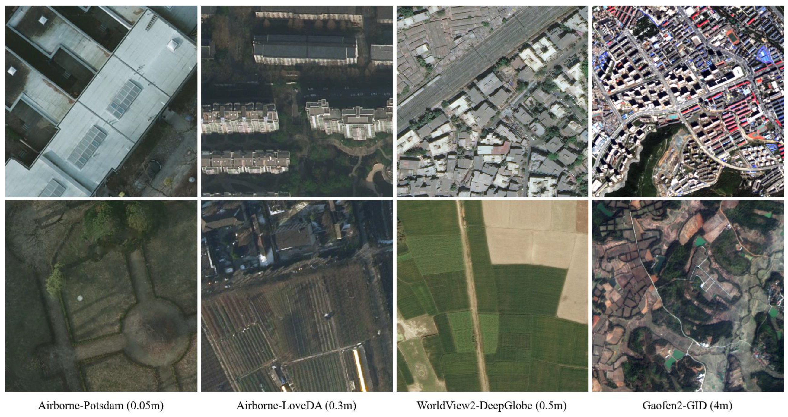
Figure 2.
Overall framework of ER-PASS for domain-incremental learning in remote sensing.
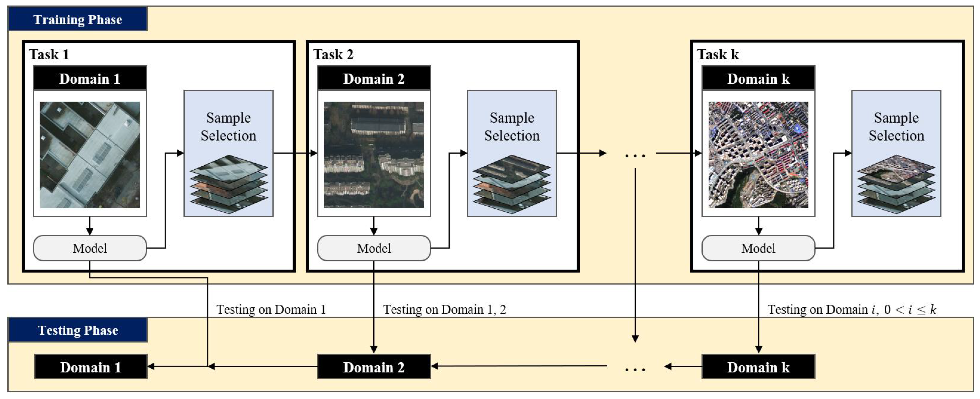
Figure 3.
Qualitative building segmentation results on each domain using the UNet model trained up to Step 4. (a) Input image; (b) Ground truth; (c) Joint; (d) EWC; (e) LwF; (f) ER; (g) Ours.
Figure 3.
Qualitative building segmentation results on each domain using the UNet model trained up to Step 4. (a) Input image; (b) Ground truth; (c) Joint; (d) EWC; (e) LwF; (f) ER; (g) Ours.
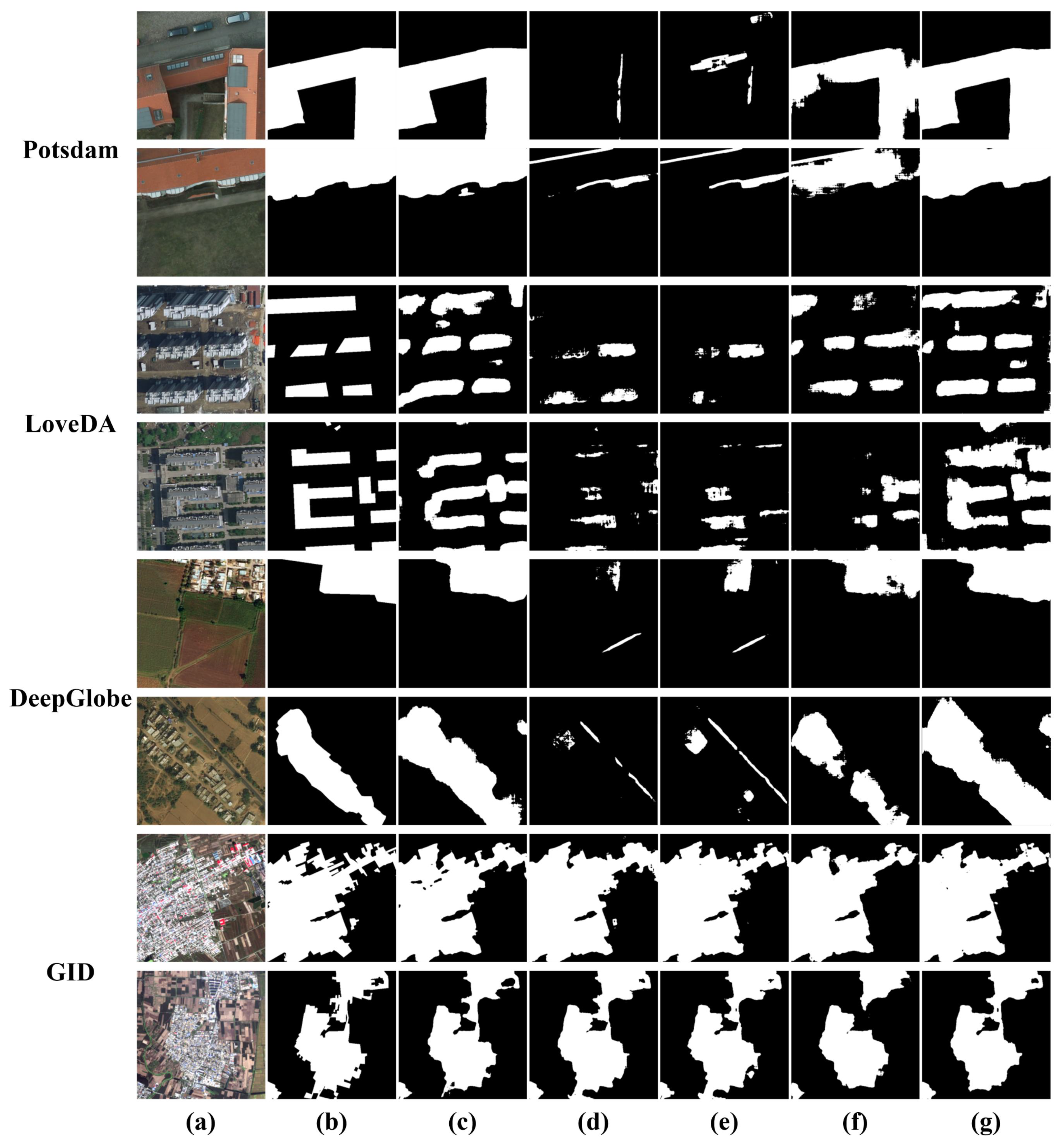
Figure 4.
Qualitative building segmentation results on the first domain using the UNet model trained at each incremental step. (a) Input image; (b) Ground truth; (c) Joint; (d) EWC; (e) LwF; (f) ER; (g) Ours.
Figure 4.
Qualitative building segmentation results on the first domain using the UNet model trained at each incremental step. (a) Input image; (b) Ground truth; (c) Joint; (d) EWC; (e) LwF; (f) ER; (g) Ours.
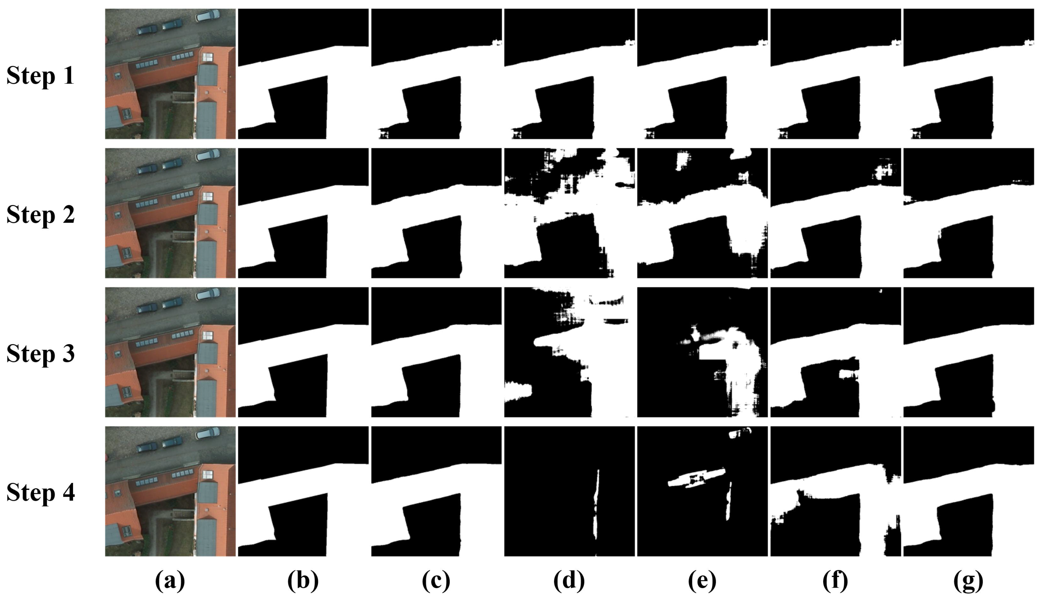
Figure 5.
Qualitative LULC classification results on each domain using the UNet model trained up to Step 4. (a) Input image; (b) Ground truth; (c) Joint; (d) EWC; (e) LwF; (f) ER; (g) Ours.
Figure 5.
Qualitative LULC classification results on each domain using the UNet model trained up to Step 4. (a) Input image; (b) Ground truth; (c) Joint; (d) EWC; (e) LwF; (f) ER; (g) Ours.
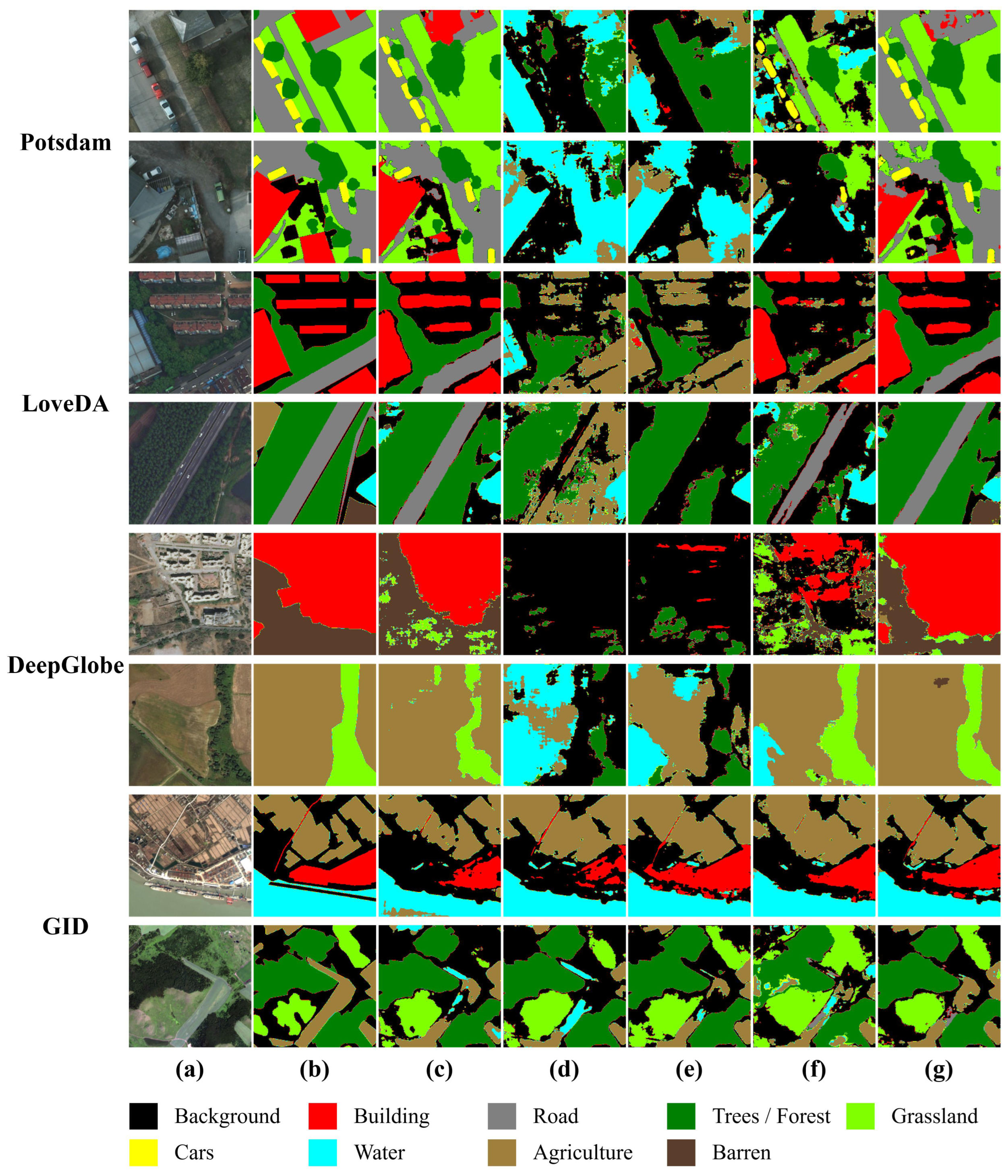
Figure 6.
Qualitative LULC classification results on the first domain using the UNet model trained at each incremental step. (a) Input image; (b) Ground truth; (c) Joint; (d) EWC; (e) LwF; (f) ER; (g) Ours.
Figure 6.
Qualitative LULC classification results on the first domain using the UNet model trained at each incremental step. (a) Input image; (b) Ground truth; (c) Joint; (d) EWC; (e) LwF; (f) ER; (g) Ours.
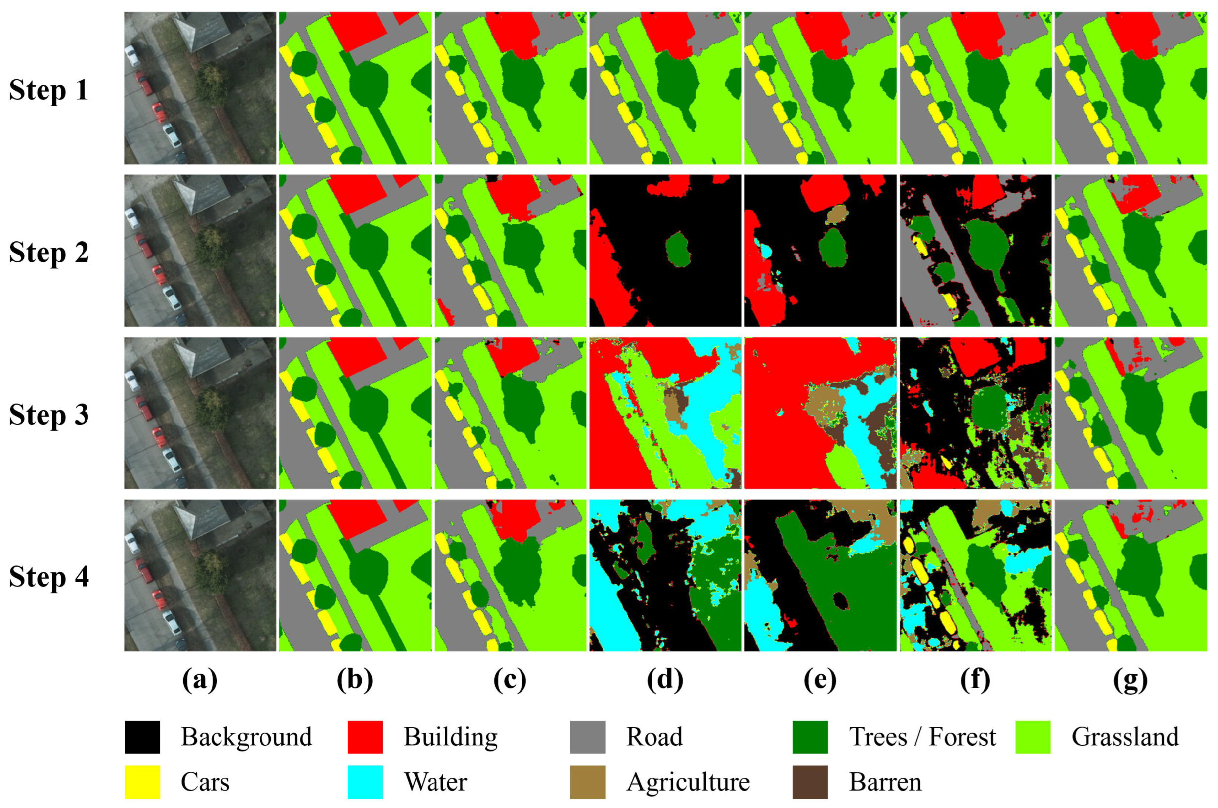
Figure 7.
Effect of sampling ratio on Backward Transfer (BWT) in incremental building segmentation with UNet.
Figure 7.
Effect of sampling ratio on Backward Transfer (BWT) in incremental building segmentation with UNet.
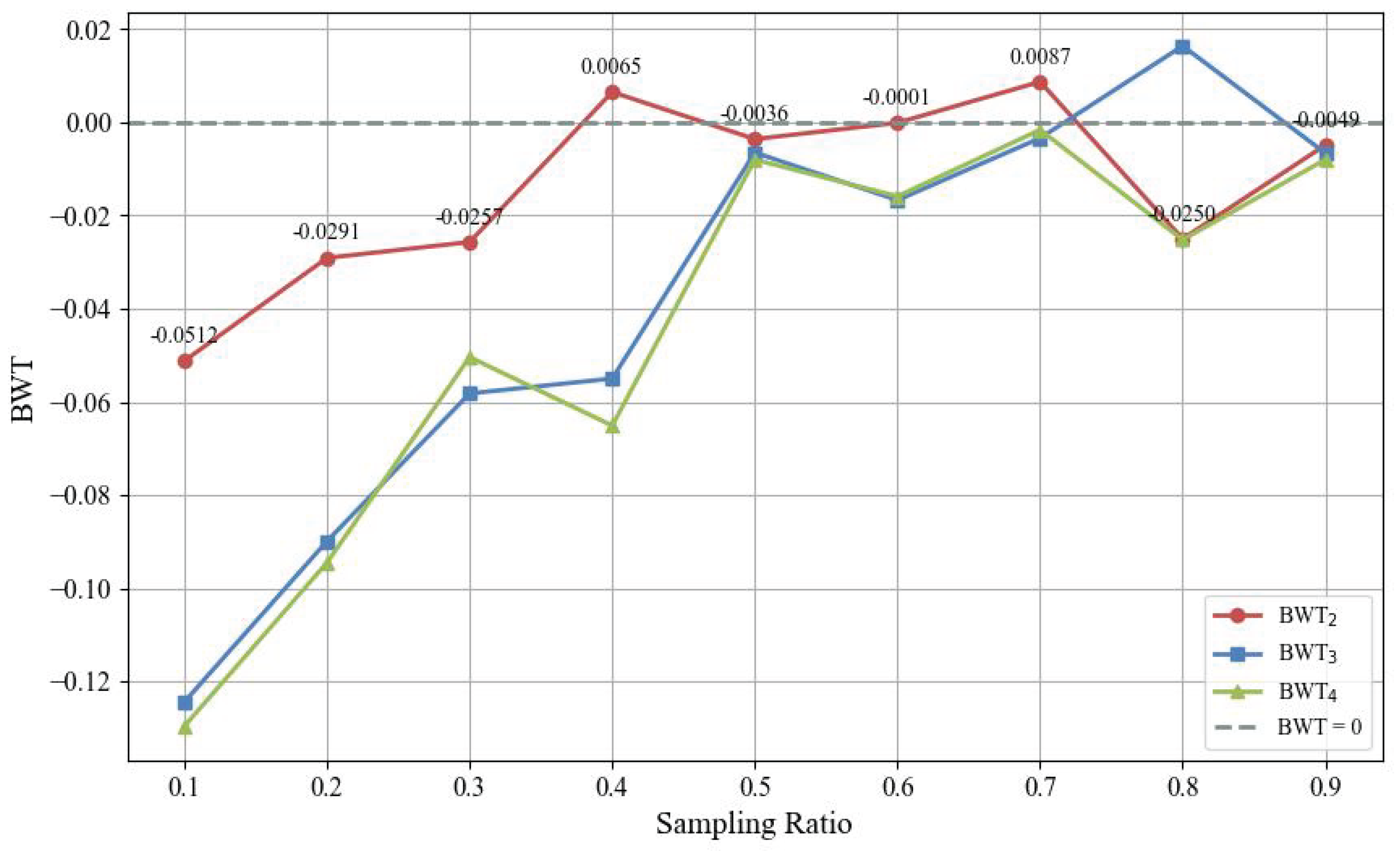

Table 1.
Description of each domain used in the sequence.
| Dataset | Platform | Resolution (m) | Stride | # of Images | Redefined Class Labels |
|---|---|---|---|---|---|
| Potsdam [56] | Airborne | 0.05 | 384 | 8,550 | Building, Road, Trees, Grassland, Cars, Background |
| LoveDA [57] | Airborne | 0.3 | 512 | 7,332 | Building, Road, Forest, Water, Agriculture, Barren, Background |
| DeepGlobe [58] | WorldView-2 | 0.5 | 968 | 7,227 | Building, Forest, Grassland, Water, Agriculture, Barren, Background |
| GID [59] | Gaofen-2 | 4.0 | 512 | 10,737 | Building, Forest, Grassland, Water, Agriculture, Background |
Table 2.
Quantitative results of UNet in incremental learning for building segmentation across four domains. The table reports IoU scores at each step, measured on all previously learned domains after training on the current task, as well as additional metrics such as AIA and BWT at the final step. ↑ indicates that a higher value is better. The best performance among the continual learning methods is highlighted in bold.
| Method | Step1 | Step2 | Step3 | Step4 | AIA4 ↑ | BWT4 ↑ | ||||||
|---|---|---|---|---|---|---|---|---|---|---|---|---|
| Potsdam | Potsdam | LoveDA | Potsdam | LoveDA | DeepGlobe | Potsdam | LoveDA | DeepGlobe | GID | |||
| Single-task | 0.8149 | 0.3672 | 0.5222 | 0.2246 | 0.2693 | 0.7391 | 0.0151 | 0.0028 | 0.0004 | 0.7276 | - | - |
| Joint learning | - | 0.8159 | 0.4761 | 0.8082 | 0.5192 | 0.7379 | 0.7859 | 0.5054 | 0.7414 | 0.6953 | 0.7078 | 0.0012 |
| Fine-tuning | - | 0.4284 | 0.5157 | 0.3032 | 0.2940 | 0.7391 | 0.0103 | 0.0102 | 0.0020 | 0.7220 | 0.4796 | |
| EWC [38] | - | 0.4300 | 0.5054 | 0.3578 | 0.2442 | 0.7386 | 0.0064 | 0.0050 | 0.0017 | 0.7175 | 0.4781 | |
| LwF [60] | - | 0.4386 | 0.5186 | 0.2664 | 0.3088 | 0.7210 | 0.0112 | 0.0168 | 0.0014 | 0.7250 | 0.4785 | |
| ER [43] | - | 0.6971 | 0.3629 | 0.5852 | 0.3854 | 0.5300 | 0.1899 | 0.2153 | 0.2827 | 0.6428 | 0.5444 | |
| Ours | - | 0.8113 | 0.4953 | 0.8157 | 0.4815 | 0.7338 | 0.8218 | 0.4703 | 0.7280 | 0.6899 | 0.7057 | |
Table 3.
Quantitative results of DeepLabV3+ in incremental learning for building segmentation across four domains. The table reports IoU scores at each step, measured on all previously learned domains after training on the current task, as well as additional metrics such as AIA and BWT at the final step. ↑ indicates that a higher value is better. The best performance among the continual learning methods is highlighted in bold.
| Method | Step1 | Step2 | Step3 | Step4 | AIA4 ↑ | BWT4 ↑ | ||||||
|---|---|---|---|---|---|---|---|---|---|---|---|---|
| Potsdam | Potsdam | LoveDA | Potsdam | LoveDA | DeepGlobe | Potsdam | LoveDA | DeepGlobe | GID | |||
| Single-task | 0.7678 | 0.4507 | 0.4859 | 0.3360 | 0.2769 | 0.7228 | 0.0216 | 0.0072 | 0.0018 | 0.7095 | - | - |
| Joint learning | - | 0.8112 | 0.4784 | 0.7987 | 0.4667 | 0.7037 | 0.7925 | 0.4526 | 0.7351 | 0.6775 | 0.6834 | 0.0101 |
| Fine-tuning | - | 0.4671 | 0.4903 | 0.3303 | 0.2930 | 0.7328 | 0.0172 | 0.0128 | 0.0045 | 0.7138 | 0.4714 | |
| EWC [38] | - | 0.4311 | 0.5267 | 0.3876 | 0.2721 | 0.7406 | 0.0126 | 0.0027 | 0.0017 | 0.7077 | 0.4737 | |
| LwF [60] | - | 0.3893 | 0.4883 | 0.3488 | 0.2779 | 0.7463 | 0.0159 | 0.0038 | 0.0047 | 0.7044 | 0.4616 | |
| ER [43] | - | 0.7075 | 0.3916 | 0.6097 | 0.3941 | 0.5545 | 0.3501 | 0.3679 | 0.4466 | 0.6584 | 0.5731 | |
| Ours | - | 0.7941 | 0.5109 | 0.8234 | 0.4475 | 0.7380 | 0.8044 | 0.4705 | 0.7149 | 0.6993 | 0.6906 | |
Table 4.
Quantitative results of UNet in incremental learning for LULC classification across four domains. The table reports mIoU scores at each step, measured on all previously learned domains after training on the current task, as well as additional metrics such as AIA and BWT at the final step. ↑ indicates that a higher value is better. The best performance among the continual learning methods is highlighted in bold.
| Method | Step1 | Step2 | Step3 | Step4 | AIA4 ↑ | BWT4 ↑ | ||||||
|---|---|---|---|---|---|---|---|---|---|---|---|---|
| Potsdam | Potsdam | LoveDA | Potsdam | LoveDA | DeepGlobe | Potsdam | LoveDA | DeepGlobe | GID | |||
| Single-task | 0.6434 | 0.1087 | 0.3611 | 0.1912 | 0.1717 | 0.5857 | 0.1114 | 0.1610 | 0.0955 | 0.6339 | - | - |
| Joint learning | - | 0.6425 | 0.3253 | 0.6304 | 0.3812 | 0.5755 | 0.6336 | 0.3928 | 0.5245 | 0.6738 | 0.5534 | 0.0019 |
| Fine-tuning | - | 0.1277 | 0.3515 | 0.1563 | 0.1610 | 0.5991 | 0.0640 | 0.1857 | 0.0845 | 0.6913 | 0.3613 | |
| EWC [38] | - | 0.1342 | 0.3705 | 0.1417 | 0.1202 | 0.6117 | 0.0659 | 0.2342 | 0.0969 | 0.6851 | 0.3645 | |
| LwF [60] | - | 0.1786 | 0.3679 | 0.1109 | 0.1098 | 0.5925 | 0.0821 | 0.2317 | 0.1829 | 0.6519 | 0.3688 | |
| ER [43] | - | 0.2925 | 0.2306 | 0.1757 | 0.2667 | 0.4220 | 0.2600 | 0.2425 | 0.3159 | 0.6173 | 0.3880 | |
| Ours | - | 0.6571 | 0.3811 | 0.6555 | 0.3710 | 0.5941 | 0.6286 | 0.3606 | 0.5272 | 0.6869 | 0.5636 | |
Table 5.
Quantitative results of DeepLabV3+ in incremental learning for LULC classification across four domains. The table reports mIoU scores at each step, measured on all previously learned domains after training on the current task, as well as additional metrics such as AIA and BWT at the final step. ↑ indicates that a higher value is better. The best performance among the continual learning methods is highlighted in bold.
| Method | Step1 | Step2 | Step3 | Step4 | AIA44 ↑ | BWT4 ↑ | ||||||
|---|---|---|---|---|---|---|---|---|---|---|---|---|
| Potsdam | Potsdam | LoveDA | Potsdam | LoveDA | DeepGlobe | Potsdam | LoveDA | DeepGlobe | GID | |||
| Single-task | 0.6354 | 0.1425 | 0.3310 | 0.1244 | 0.1325 | 0.5391 | 0.0540 | 0.1962 | 0.1528 | 0.5630 | - | - |
| Joint learning | - | 0.6300 | 0.3110 | 0.6289 | 0.3602 | 0.6191 | 0.5886 | 0.3652 | 0.5638 | 0.6530 | 0.5462 | |
| Fine-tuning | - | 0.1320 | 0.3795 | 0.1466 | 0.1537 | 0.5799 | 0.0729 | 0.2002 | 0.1457 | 0.6563 | 0.3633 | |
| EWC [38] | - | 0.1769 | 0.3570 | 0.1618 | 0.1789 | 0.6125 | 0.0649 | 0.2018 | 0.1567 | 0.6679 | 0.3732 | |
| LwF [60] | - | 0.1853 | 0.3550 | 0.2107 | 0.1504 | 0.5083 | 0.0774 | 0.2568 | 0.2265 | 0.6069 | 0.3718 | |
| ER [43] | - | 0.3567 | 0.3142 | 0.3565 | 0.2866 | 0.3675 | 0.3537 | 0.3205 | 0.4240 | 0.5443 | 0.4296 | |
| Ours | - | 0.6275 | 0.3446 | 0.5908 | 0.3441 | 0.5805 | 0.5297 | 0.3521 | 0.5407 | 0.6164 | 0.5341 | |
Table 6.
Results of the ablation study on the proposed sample selection algorithm in incremental building segmentation with UNet.
Table 6.
Results of the ablation study on the proposed sample selection algorithm in incremental building segmentation with UNet.
| Method | Submodular | Eval. Score | Score Function | AIA4 | BWT4 |
|---|---|---|---|---|---|
| Random | ✗ | ✗ | Random | 0.6907 | |
| Submodular | ✓ | ✗ | 0.6796 | ||
| Eval. Score | ✗ | ✓ | S | 0.6930 | |
| Ours | ✓ | ✓ | 0.7057 |
Table 7.
Comparison of training time and memory usage at Step 4 of incremental building segmentation with UNet.
Disclaimer/Publisher’s Note: The statements, opinions and data contained in all publications are solely those of the individual author(s) and contributor(s) and not of MDPI and/or the editor(s). MDPI and/or the editor(s) disclaim responsibility for any injury to people or property resulting from any ideas, methods, instructions or products referred to in the content. |
© 2025 by the authors. Licensee MDPI, Basel, Switzerland. This article is an open access article distributed under the terms and conditions of the Creative Commons Attribution (CC BY) license (http://creativecommons.org/licenses/by/4.0/).
Copyright: This open access article is published under a Creative Commons CC BY 4.0 license, which permit the free download, distribution, and reuse, provided that the author and preprint are cited in any reuse.


