Submitted:
19 July 2025
Posted:
22 July 2025
You are already at the latest version
Abstract
In a stage of more and more complex and high-frequency financial markets, the volatility analysis is a cornerstone of modern financial econometrics with practical applications in portfolio optimization, derivative pricing and systematic risk assessment. This paper introduces a novel Bayesian Time-varying Generalized Autoregressive Conditional Heteroskedasticity (BtvGARCH-Itô) model designed to improve the precision and flexibility of volatility modeling in financial markets. Original GARCH-Itô models, while effective in capturing realized volatility and intraday patterns, rely on fixed or constant parameters thus it is limited to study structural changes. Our proposed model addresses this restraint by integrating the continuous-time Ito process with time-varying Bayesian inference to allow parameters to vary over time based on prior beliefs to quantify uncertainty and minimize overfitting especially in small-sample or high-dimensional settings. Through simulation studies using sample sizes of N=100 and N=200, we find that BtvGARCH-Itô outperformed original GARCH-Itô in-sample fit and out-of-sample forecast accuracy based on posterior estimates comparison with true parameter values and forecasting error metrics. For the empirical validation, this model is applied to analyze volatility of S&P500 and Bitcoin (BTC) using one minute length data for S&P500 (from 2023-01-03 to 2024-12-31) and BTC (from 2023-01-01 to 2025-01-01). This model has a potential as a robust tool and new direction in volatility modeling for financial risk management.
Keywords:
volatility analysis
; S&P500
; BTC
; BtvGARCH-Itô
Introduction
Modeling financial asset volatility is very important for option pricing, managing risk, and building investment portfolios (Opschoor and Lucas, 2023; Engle and Gallo, 2006). GARCH models introduced by Engle (1982) and Bollerslev (1986) are commonly used to track how volatility changes over time. These models use daily squared returns to estimate volatility. However, they rely on limited information which makes them less effective in catching market behavior. Fan and Wang (2007) argued that high-frequency financial data has improved how we measure volatility and forecasting performance. New measures like realized variance, bipower variation, realized kernel, intraday range, and multipower variation use detailed intraday returns are found in the existing literature including Barndorff-Nielsen et al. (2004), Barndorff-Nielsen et al. (2008), Todorov (2009), Carr and Wu (2003), and Huang and Tauchen (2005). These measures produce less biased estimates of volatility under the right conditions (Andersen, Bollerslev and Diebold, 2007).
Realized Generalized Autoregressive Conditional Heteroskedasticity (GARCH) models (Song et al., 2020; Kim and Wang, 2016) have constructed on these improvements. They model both returns and realized volatility together. One key part of these models is the measurement equation which links realized volatility directly to the model's estimate of true volatility. This setup improves performance compared to traditional GARCH models, for example, Song et al. (2020) accounts both price jumps and volatilities. Realized GARCH-Itô models include more detailed data like integrated volatility and jump variation and it helps the models capture unexpected changes in prices. Realized GARCH-Itô models predict volatility better than earlier models (Kim and Wang, 2016) accounting intraday U-shape volatility.
While significant progress has been made, these models assume constant and use fixed parameters. This is a problem because financial markets are dynamic and change significantly over time. The concept of time varying coefficients has been increasingly agreed in econometric models to help deal with this sort of issue. They let parameters adjust to varying market conditions and improve predictions during uncertain periods of structural changes or economic shocks or even policy shifts. In fact, financial markets are constantly changing. Time-varying models are also identifying shifts in market dynamics and correlations (Andersen and Bollerslev, 1997; Andersen, Thyrsgaard and Todorov, 2019; Opschoor and Lucas, 2023). For example, time-varying GARCH coefficients shows how the second order dynamics of U.S. stock market changed sharply after 2001 internet bubble burst while Chinese market remained isolated (Gao, Peng, Wu and Yan, 2024). These models are effective in volatility predictions of future return distributions and risk measures. Besides, they can handle non stationarity of which is common in financial data.
In addition to time-varying models, Bayesian models treat all uncertainty as probability based on prior beliefs about how parameters might change over time. Furthermore, Bayesian inference estimates all unknown parameters while showing how they might relate to each other. They are also beneficial when dealing with small datasets, and even prevent overparameterization in high dimensional settings. The combination of Bayesian inference to time-varying parameter models resulted in efficient posterior and improved forecasting accuracy (Koop and Korobilis, 2020; Taspinar et al., 2021; Kalli and Griffin, 2014; Jacquier, Polson and Rossi, 2004). Using Bayesian methods together with time-varying parameters provides the effectiveness of modeling and volatility forecasting.
Given the importance and the need to adapt to continuous changing financial markets, this paper introduces a Bayesian Time-varying Realized GARCH-Itô (BtvGARCH-Itô) model. This model lets parameters vary over time, fits high frequency data more effectively and reduces uncertainty by using prior knowledge to improve accuracy of volatility analysis in financial markets.
2. Realized GARCH-Itô Model
The realized GARCH-Itô model first introduced by Song et al. (2020) presents a significant advancement in volatility analysis by integrating high frequency financial data with continuous-time jump-diffusion processes. This hybrid model extends the united GARCH-Itô framework of Kim and Wang (2016) by incorporating realized volatility (RV) and jump variation (JV) as innovations. Thereby, Song et al. (2020) filled the gap between discrete-time econometric models and continuous time stochastic processes. It is particularly effective to account dynamic change of volatility in financial markets including high frequency data analysis whereas market noises, price jumps and intraday volatility patterns exist. Realized GARCH-Itô model is formulated as a stochastic differential equation. The log stock price process for follows:
Where is the drift, is the instantaneous volatility, is a Brownian motion, is jump sizes, and is a counting process for jumps. At integer times n, the conditional variance is:
Where , , , and the integrated volatility over [n – 1, n] is:
With
Where is the latent conditional variance at time t, is the baseline volatility, is lagged realized volatility (), is lagged jump variation (), is lagged variance of latent volatility, and = (,, parameters are assumed constant over time following a normal distribution.
The quasi-likelihood function used for static parameters in this model is stated as:
Where , and subject to .
3. Bayesian Time-Varying GARCH-Itô Model
The Bayesian Time-varying GARCH-Itô (BtvGARCH-Itô) model extends the Generalized unified GARCH-Itô model by incorporating time-varying paramters and Bayesian inference to study dynamic volatility in high-frequency financial markets. This section delivers the BtvGARCH-Itô model specification which is objected to effectively estimate the latent volatility and its time-varying components using observed realized volatility, jump variation impact and lagged variance within a Bayesian inference framework. This model is suitable to financial applications of high-frequency data analysis where volatility dynamics swing continuously. The BtvGARCH-Itô model defines the latent volatility process { as follows:
For t=1
Where is a small constant ensuring positivity, and is a constant derived from the empirical distribution of jump variation .
For t=2,…,N
Where is the realized volatility, is the jump variation, and are time-varying parameters satisfying The time-varying parameters shifts via a Gaussian random walk in logit space:
Where and . The measurement equation is:
To complete the Bayesian specification, we assign prior distributions as follows:
Initial coefficients:
Where is the half-Cauchy distribution adjusted at 0 with scale b, and ( are prior mean and standard deviation hyperparameters.
Innovation standard deviations:
Random walk innovations:
The Bayesian posterior of this model can be written as:
We provide the implementation details of the BtvGARCH-Itô model in RStudio software in the supplementary material.
4. Simulation Study
4.1. Data Generation Process
We simulated synthetic data for N=100 and N=200 time points to evaluate the model’s finite sample performance. The jump variation process JV was generated as independent draws from a uniform distribution on [0, 0.2] with the median value denoted by . The time-varying parameters ,, were defined to vary smoothly over time according to sinusoidal functions to mimic realistic dynamics. The latent volatility was computed recursively as follows:
With and
4.2. Simulation Results
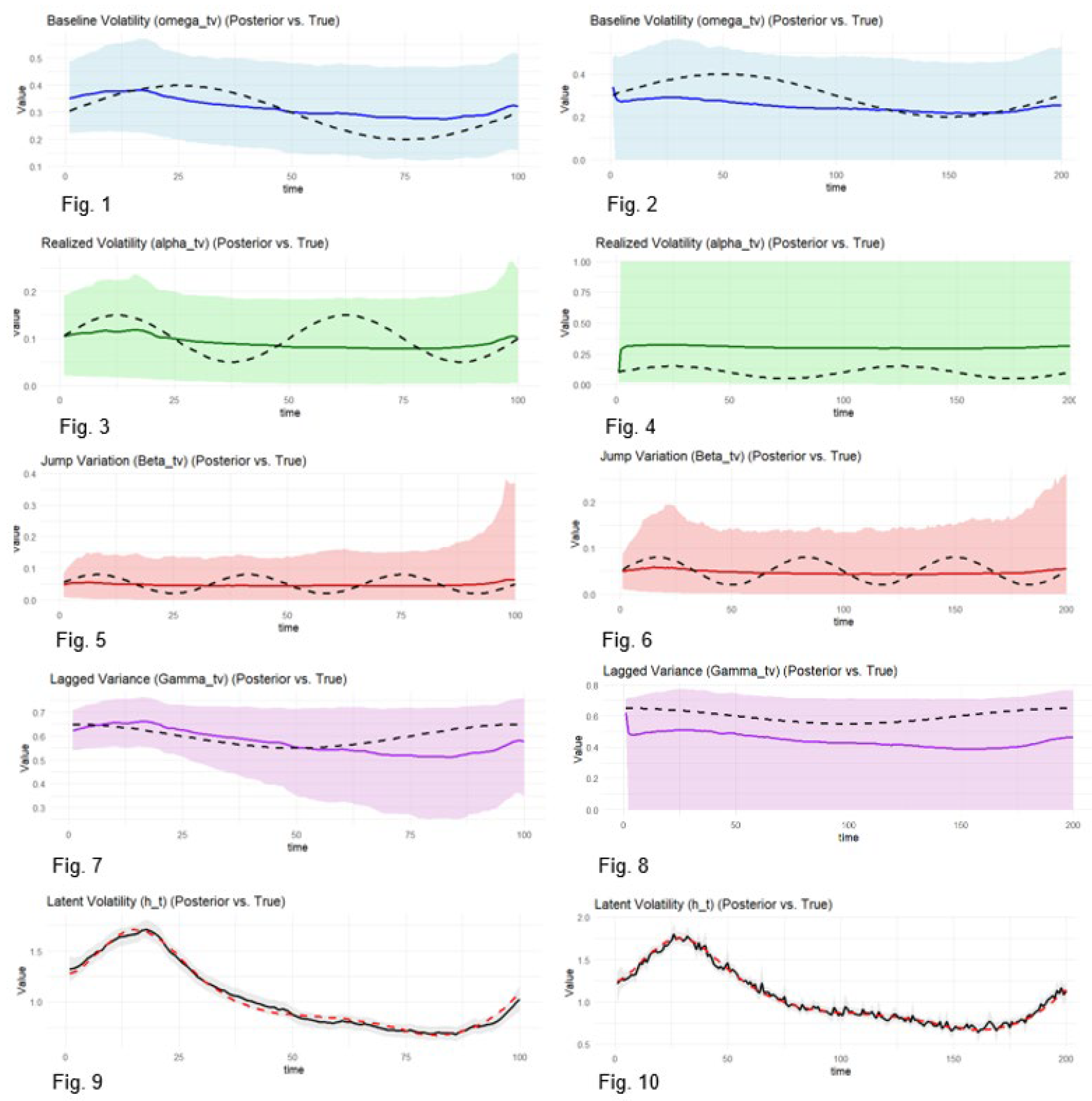
This section provides the estimated simulation results from GARCH-Itô and BtvGARCH-Itô models for two simulated data sample sizes. Table 1 shows the posterior means of static parameters, posterior intervals, R hat estimates and effective sample sizes. Figures 1 to 10 present the posterior time varying estimates of means and 95 percent incredible intervals of parameters. Table 2 reports model prediction accuracy metrics for two models. Overall, these simulation results demonstrate that the BtvGARCH-Itô is capable of more accurately estimating volatilities under realistic synthetic dataset. Besides, this model can be used to estimate both static and time varying coefficients thus, it supports practical application to volatility analysis in empirical financial markets.

Table 3.
Model Accuracy Metrics: GARCH-Itô vs. Bayesian Time-varying GARCH-Itô.
| N=100 | N=200 | |||||||||||
| Parameter | GARCH-Itô | BtvGARCH-Itô | GARCH-Itô | BtvGARCH-Itô | ||||||||
| MAE | MSE | RMSE | MAE | MSE | RMSE | MAE | MSE | RMSE | MAE | MSE | RMSE | |
| 0.1133 | 0.0128 | 0.1133 | 0.0432 | 0.00242 | 0.0492 | 0.1385 | 0.0191 | 0.1385 | 0.0469 | 0.0028 | 0.0529 | |
| 0.0632 | 0.0039 | 0.0632 | 0.0289 | 0.0011 | 0.0339 | 0.0442 | 0.0019 | 0.0442 | 0.0346 | 0.0019 | 0.0440 | |
| 0.0499 | 0.0024 | 0.0499 | 0.0198 | 0.0004 | 0.0218 | 0.0499 | 0.0024 | 0.0499 | 0.0188 | 0.0004 | 0.0212 | |
| 0.0072 | 0.0000 | 0.0071 | 0.0440 | 0.0033 | 0.0575 | 0.1413 | 0.0199 | 0.1413 | 0.0419 | 0.0023 | 0.0489 | |
| 0.0568 | 0.0085 | 0.0922 | 0.0299 | 0.0012 | 0.0348 | 0.0535 | 0.0072 | 0.0848 | 0.0192 | 0.006 | 0.0253 | |
Notes: Table 3 provides the forecast accuracy of both original GARCH-Itô and BtvGARCH-Itô models based on three error metrics: Mean Absolute Error (MAE), Mean Squared Error (MSE) and Root Mean Squared Error (RMSE). Accuracy is assessed for each key parameter and for the latent volatility using simulated samples N = 100 and N=200. These results revealed that the BtvGARCH-Itô model achieves lower errors compared to original GARCH-Itô.
Figures 1–10.
Time-varying posterior means of parameters estimated by BtvGARCH-Itô Model. Notes: Figures 1 to 10 illustrate the time varying posterior means of parameters, omega (, alpha (), Beta (), Gamma ( and latent variance or factor () estimated from the BtvGARCH-Itô model for simulated datasets with time lengths t=100 and t=200. The solid lines present true parameter values that being used to generate the data and dashed lines represent the time-varying posterior mean estimates.
5. Empirical Study
This section provides the empirical application of BtvGARCH-Itô model to two financial assets namely S&P500 and Bitcoin using one-minute intraday returns time series data. The study sample periods for S&P500 ranges from 2023-01-03 to 2023-12-31 and for Bitcoin covers from 2023-01-01 to 2025-01-01. S&P500 is considered to be highly liquid equity stock and Bitcoin (BTC) as a volatile and speculative digital asset. The selection of these two markets is to reflect different market structures. This model assesses its capability to model latent volatility dynamics across two markets.
For the case of S&P500 (Table 4), it shows a strong empirical support for the model’s effectiveness in studying main features of volatility dynamics in a stable financial market. The static posterior intercept () which sets the baseline level of conditional volatility is estimated at . The estimated average volatility level is low which is consistent with the relatively stable U.S. equity market during the study period. The static posterior coefficient of realized volatility () is 0.0479. This value indicates a moderate impact of realized measures on volatility dynamics in the well-regulated market. The static posterior means of jump variation () is 0.0324, which assesses the influence of discontinuous price jumps on current volatility. The small positive value revealed that price jumps in S&P500 has a small effect on the overall volatile. The static posterior means estimated for lagged variance () is 0.598 which measures the persistence of latent volatility.
For the case of Bitcoin (Table 5), the static intercept posterior means for parameter () is . The estimated average volatility level is much larger than in S&P500 index during the study period. This indicates how Bitcoin remains a speculative and risk-sensitive asset. The static posterior coefficient of realized volatility () is 0.0642 which also exceeds that of the S&P500. This finding highlights Bitcoin’s high volatility reactivity to incoming market information. The static posterior means of jump variation () is 0.00245 which is substantially lower than S&P500 estimates. This result suggests that persistent price jumps contribute least to latent volatility. One possible reason is that the baseline and RV already absorb most of high frequency variation. The static posterior means estimated for lagged variance () is 0.573 which is slightly less than in the equity market S&P500. However, the larger baseline volatility in BTC highlights the adaptability of the model to differentiate the nature of high risk and stable financial markets.
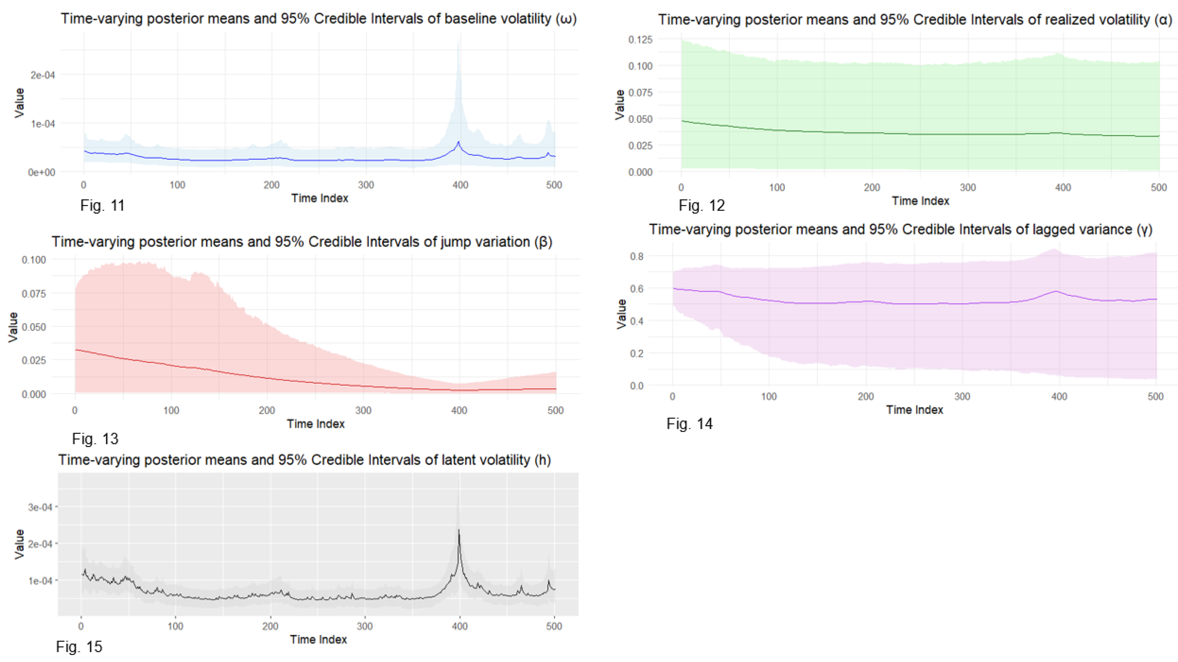
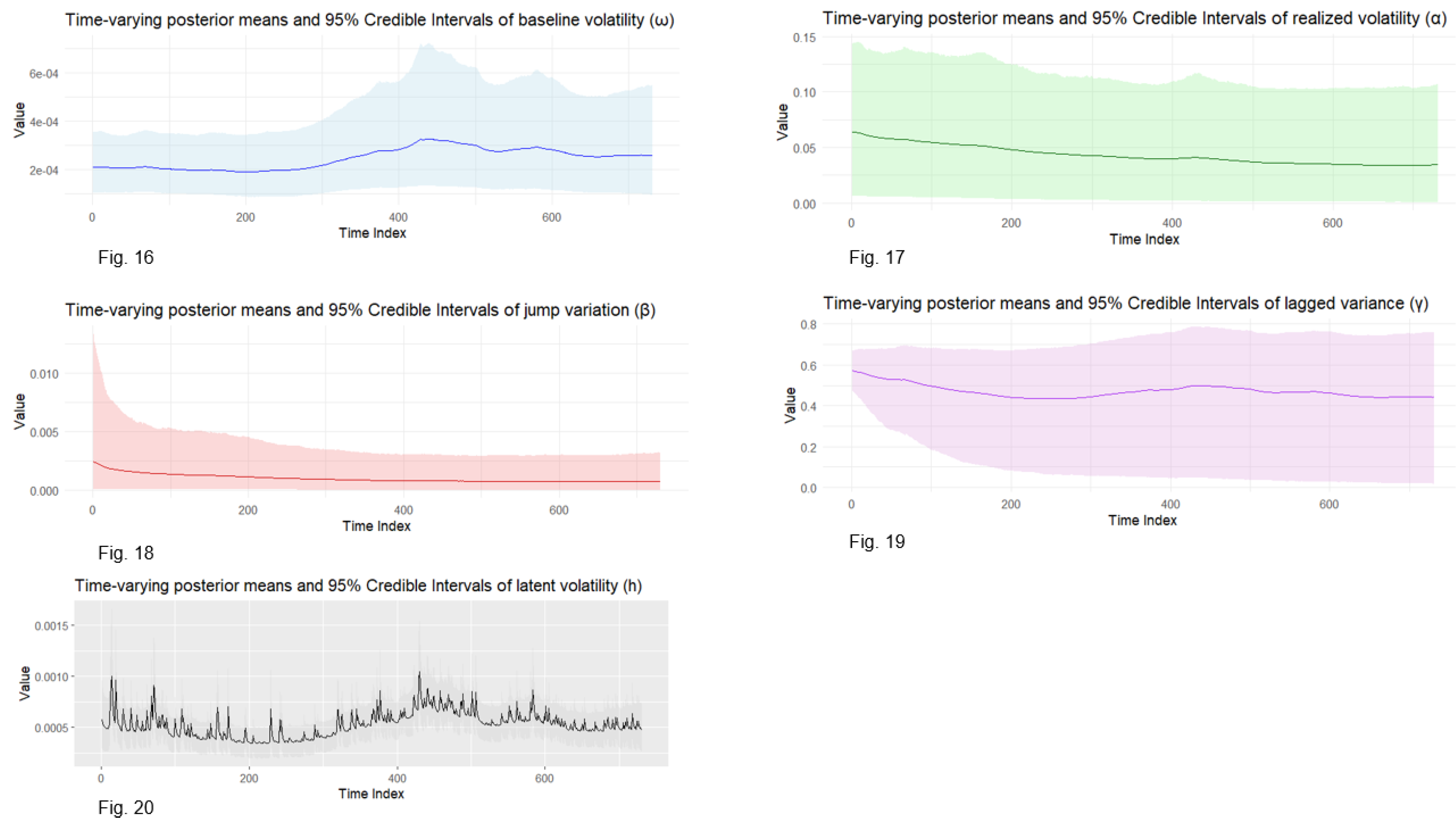
While the estimated static posterior means of parameters present fixed volatility of the market, it proves overly restrictive in high-frequency data and continuous changing financial environments. This model addresses this by allowing parameters vary over time to more accurately examine dynamic nature of investor behaviour, risk perceptions and volatility transmission mechanisms. The time-varying estimates of parameters including latent volatility are provided in Figures 11-15 for S&P500 and Figures 16-20 for Bitcoin. With this method on modeling volatility persistence and shifts, investors can benefit from value-at-risk estimation and derivative pricing. The evidence from both assets supports the conclusion that while static models reveal the overall market behaviour, time-varying models report unexpected shifts in volatility drivers that affect market-risk. In sum, the empirical evidence validates the efficacy of BtvGARCH-Itô model in analysing dynamic volatility structures across both traditional and digital financial assets.
Figures 11–15.
Time-varying posterior means and 95% credible intervals of volatilities of S&P500 (2023-01-03 to 2024-12-31). Notes: Figures 11–15 present the time-varying posterior means (solid lines) and 95% credible intervals (shaded areas) for all parameters estimated from the BtvGARCH-Itô model using 1-minute close prices of the S&P500.
Figures 16–20.
Time-varying posterior means and 95% credible intervals of volatilities of Bitcoin (2023-01-01 to 2025-01-01). Notes: Figures 16–20 present the time-varying posterior means (solid lines) and associated 95% credible intervals (shaded areas) for key volatility-related parameters estimated from the BtvGARCH-Itô model using 1-minute close prices of Bitcoin (BTC).
6. Conclusions
This paper develops and empirically validates a Bayesian Time-Varying Realized GARCH-Itô model, a novel framework that integrates discreate-time GARCH dynamics with continuous-time Itô processes and time-varying coefficients within Bayesian inference. This model advanced volatility modeling because it allows model parameters to vary over time. Unlike original GARCH-Itô models that assume static coefficients, this BtvGARCH-Itô model enables joint inference on both static and time-varying posterior distributions. Besides, this model offers a more flexible and accurate classification of volatility shifts through the use of latent stochastic components estimated for financial markets. This new model adds a significant contribution to the field of financial econometrics and financial volatility analysis.
Simulation studies conducted for sample sizes N = 100 and N = 200 determine how well this model recover both static and time-varying parameters. In particular, the Bayesian posterior estimates closely track the true latent volatility path. The estimated simulation results confirmed that the BtvGARCH-Itô model grasps greater in-sample fit and out-of-sample forecast accuracy. This is evident in its closer alignment with true parameter values and lower error metrics (MAE, MSE, RMSE) compared to the original GARCH-Itô specification (Song et al., 2020). This model is also capable of tracking volatility shifts and identifying distinct volatility spikes linked to market shocks in the empirical application of volatility analysis of S&P500 intraday returns. Besides, its application to Bitcoin returns demonstrates that the BtvGARCH-Itô can be applied to markets with heavy tails and frequent jumps.
Overall, this model offers a statical tool for risk management and portfolio allocation in modern financial markets. It unifies time-varying parameters of realized volatility and jump variation within a full Bayesian posterior framework.
The BtvGARCH-Itô is just the first step and several directions remain open. In financial markets, assets move together so that extending this model to a multivariate setting would benefit further for volatility spillovers and co-jumps which are essential for portfolio risk assessment and cross-asset dynamics for investors. In practical applications, fixed bandwidth might limit flexibility thus, allowing data-driven bandwidths could improve the accuracy of time-varying coefficient estimates. As fat tails exist in financial returns, incorporating heavy tailed or skewed distributions, for example, Student-t distribution may better catch extreme events or price jumps.
Supplementary Materials
The model implementation in RStudio Software is available at Preprint.org.
Author Contributions
Authors contributed equally to this work.
Funding
Faculty of Economics, Chiang Mai University, Chiang Mai 50200, Thailand
Data Availability Statement
The empirical analysis in this study utilizes secondary data obtained from Yahoo Finance. Specifically, we downloaded intraday price data at 1-minute intervals and computed log returns based on closing prices.
Acknowledgments
The authors have thoroughly reviewed and edited all content generated during the preparation of this manuscript and take full responsibility for its accuracy and conclusions. This study used only publicly available data and did not require ethical approval. Grok AI was used only for grammar and language improvement.
Conflicts of Interest
None.
Appendix A
Figure A1.
S&P500 Close Prices (1-minute frequency data) from 2023-01-03 to 2024-12-3.
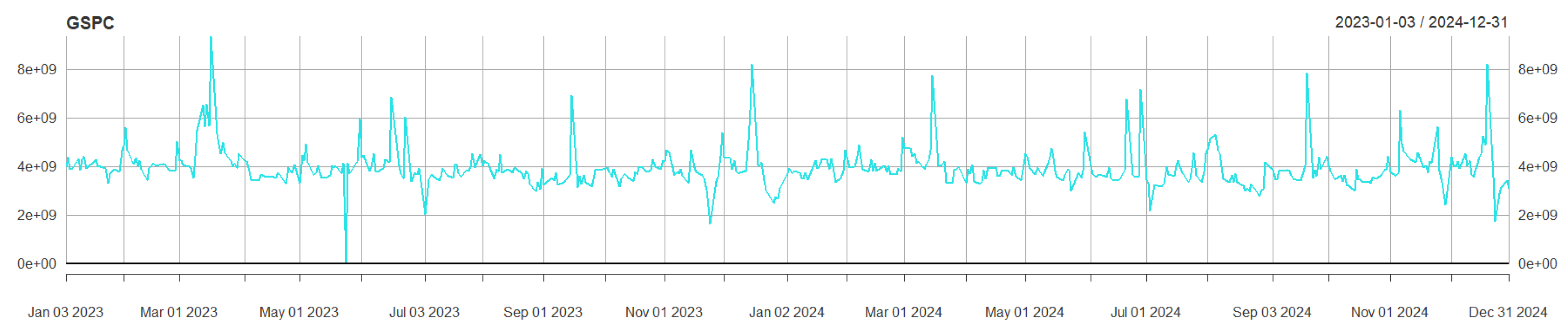
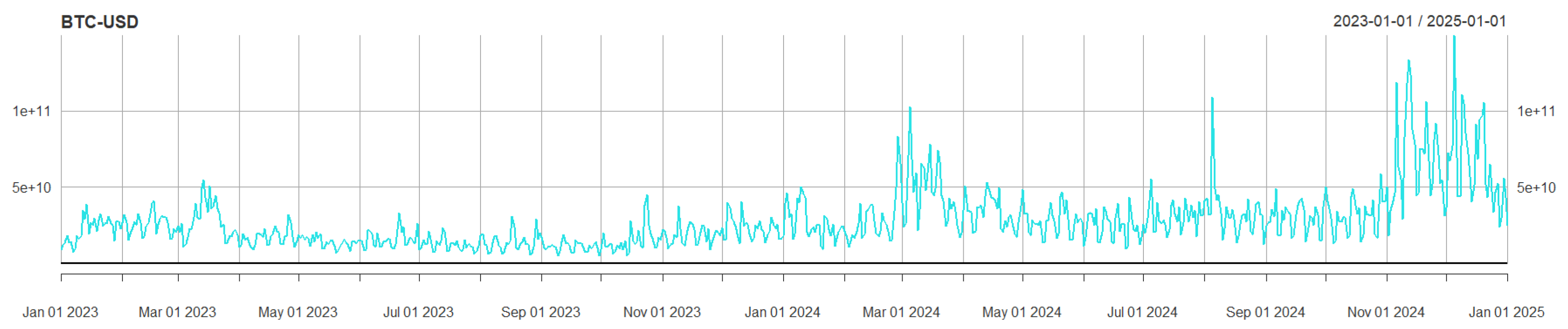
Figure A2.
Bitcoin Close Prices (1-minute frequency data) from 2023-01-03 to 2024-12-3.
Appendix B. Theorems and Proofs
Theorem 1
. Positivity and Boundedness of the Latent Volatility Process
Assume , , for some and . Then, the latent volatility process {satisfies:
Proof of Theorem 1
. We prove positivity and boundedness by induction.
Base case (t=1): The initial volatility is:
Since and , we have . For boundedness:
Where since and is a finite constant.
Assume . For
Since , and , it follows that . For boundedness:
Iterate the inequality:
Continuing to t=1, we obtain:
Since <1, the series converges. Bounding each term:
Then, we get:
The geometric series converges since :
Thus:
Where . Hence, is positive and bounded.
Theorem 2.
Properness of the Bayesian Posterior Distribution.
Given priors , , , , and , and the posterior:
is proper, i. e., .
Proof of Theorem 2
. The joint posterior is:
Likelihood: The Gaussian likelihood is continuous and bounded for and is finite by Theorem 1. Thus, it is integrable over any compact interval .
Volatility Process: The Dirac delta imposes deterministic recursion.
Thus, integrating out contributes to 1.
Priors: Initial parameters are proper, the logit transformation ensures and time-varying function follows a Gaussian random walk () which defines a proper transition density.
Theorem 3.
Identifiability of Time-Varying Parameters. The mapping is injective almost surely. That is, if , then with probability 1.
Proof of Theorem 3.
Let . Let be the smallest index where .
Case =1;
This function f() is continuously differentiable with non-zero partial derivatives (since and the denominator is positive), hence implies .
Case : for t < , assume at t=.
Since and , the linear combination differs for almost all , that implies . Since implies N () N (), so almost surely.
Theorem 4.
Posterior Consistency under True Data Generation Process. (Let { be generated from the true BtvGARCH-Itô process: , with true latent parameters . Suppose the prior : over assign positive density in every open neighborhood of (, the likelihood p( is continuous in (, the parameter space is compact and the model is identifiable as shown in Theorem 3. Then, the posterior distribution satisfies:
i.e., the posterior weakly converges to a Dirac delta at the true parameters.
Proof of Theorem 4
. We apply the posterior consistency result from Theorem 2.1 of Ghosal, Ghosh and van der Vaart (2000) which provides sufficient conditions under which Bayesian posterior lies on the true parameter values. Let Θ denote the parameter space for ( and let be the prior. Let the posterior be defined as:
Under the following conditions:
- (i)
- The true parameter values () lie in the support of the prior
- (ii)
- The likelihood is continuous in (
- (iii)
- The parameter space is compact via logit transform and
- (iv)
- The model is identifiable (Theorem 3)
Then, the posterior distribution satisfies weak consistency:
References
- Andersen, T. G., Thyrsgaard, M. and Todorov, V. (2019). Time-Varying Periodicity in Intraday Volatility. Journal of the American Statistical Association, 114(528), 1695-1707. [CrossRef]
- Andersen, T. G. and Bollerslev, T. (1997). Intraday periodicity and volatility persistence in financial markets. Journal of Empirical Finance, 4, 115-158. [CrossRef]
- Andersen, T. G., Bollerslev, T. and Diebold, F. X. (2007). ROUGHING IT UP: INCLUDING JUMP COMPONENTS IN THE MEASUREMENT, MODELING, AND FORECASTING OF RETURN VOLATILITY. The Review of Economics and Statistics, 89(4), 701-720.
- Barndorff-Nielsen, O. E., Hansen, P. R., Lunde, A. and Shephard, N. (2008). Designing realized kernels to measure ex-post variation of equity prices in the presence of noise. Econometrica, 76(6), 1481–1536. [CrossRef]
- Barndorff-Nielsen, O. E. and Shephard, N. (2004). Power and bipower variation with stochastic volatility and jumps. Journal of Financial Econometrics, 2(1), 1–37. [CrossRef]
- Bollerslev, T. (1986). Generalized autoregressive conditional heteroskedasticity. Journal of Econometrics, 31(3), 307-327. [CrossRef]
- Carr, P. and Wu, L. (2003). What type of process underlies options? A simple robust test. The Journal of Finance, 58(6), 2581–2610. [CrossRef]
- Engle, R. F. and Gallo, G. M. (2006). A multiple indicators model for volatility using intra-daily data. Journal of Econometrics, 131, 3-27. [CrossRef]
- Engle, R. F. (1982). Autoregressive Conditional Heteroscedasticity with Estimates of the Variance of United Kingdom Inflation. Econometrica, 50(4), 987-1007. https://www.jstor.org/stable/1912773.
- Gao, J., Peng, B., Wu, W. B. and Yan, Y. (2024). Time-varying multivariate causal processes. Journal of Econometrics, 240, 105671. [CrossRef]
- Ghosal, S., Ghosh, J. K., and van der Vaart, A. W. (2000). Convergence Rates of Posterior Distributions. Annals of Statistics, 28(2), 500–531. [CrossRef]
- Huang, X. and Tauchen, G. T. (2005). The relative contribution of jumps to total price variance. Journal of Financial Econometrics, 3(4), 456–499. [CrossRef]
- Opschoor, A. and Lucas, A. (2023). Time-Varying variance and skewness in realized volatility measures. International Journal of Forecasting, 39, 827-840. [CrossRef]
- Song, X., Kim, D., Yuan, H., Cui, X., Lu, Z., Zhou, Y. and Wang, Y. (2020). Volatility Analysis with Realized GARCH-Ito Models. Journal of Econometrics, 222 (1), 393-410. [CrossRef]
- Todorov, V. (2009). Estimation of continuous-time stochastic volatility models with jumps using high-frequency data. Journal of Econometrics, 148, 131-148. [CrossRef]
- Taspinar, S., DoGan, O., Chae, J. and Bera, A. K. (2021). Bayesian Inference in Spatial Stochastic Volatility Models: An Application to House Price Returns in Chicago. Oxford Bulletin of Economics and Statistics, 83(5), 1243-1272. [CrossRef]
- Jacquier, E., Polson, N. G. and Rossi, P. E. (2004). Bayesian analysis of stochastic volatility models with fat-tails and correlated errors. Journal of Econometrics, 122(1), 185-212. [CrossRef]
- Kalli, M. and Griffin, J. E. (2014). Time-varying sparsity in dynamic regression models. Journal of Econometrics, 178(2), 779-793. [CrossRef]
- Koop, G. and Korobilis, D. (2022). BAYESIAN DYNAMIC VARIABLE SELECTION IN HIGH DIMENSIONS. International Economic Review, 64(3), 1047-1074. [CrossRef]
- Kim, D. and Wang. (2016). Uni ed Discrete-Time and Continuous-Time Models and Statistical Inferences for Merged Low-Frequency and High-Frequency Financial Data. Journal of Econometrics, 194(2), 220-230. [CrossRef]
Table 1.
Posterior means, standard deviations, credible intervals, values, and effective sample sizes.
Table 1.
Posterior means, standard deviations, credible intervals, values, and effective sample sizes.
| Data | Parameter | Mean | Std. Dev. | q5 | q95 | Bulk-ESS | Tail-ESS | |
| -44.4 | 14.7 | -69 | -20.5 | 1.00 | 1608 | 2191 | ||
| 0.353 | 0.0667 | 0.243 | 0.462 | 1.00 | 2932 | 2605 | ||
| 0.106 | 0.0419 | 0.0375 | 0.177 | 1.00 | 2752 | 2037 | ||
| 0.0479 | 0.0197 | 0.0163 | 0.0805 | 1.00 | 3811 | 1606 | ||
| 0.622 | 0.0430 | 0.552 | 0.692 | 1.00 | 4132 | 2806 | ||
| N=100 | 0.0517 | 0.0335 | 0.00449 | 0.111 | 1.01 | 872 | 1424 | |
| 0.100 | 0.154 | 0.00626 | 0.260 | 1.00 | 1538 | 1820 | ||
| 0.297 | 2.17 | 0.00662 | 0.754 | 1.00 | 3653 | 2416 | ||
| 0.0535 | 0.0328 | 0.00575 | 0.112 | 1.02 | 572 | 1300 | ||
| 0.0994 | 0.00823 | 0.0866 | 0.114 | 1.00 | 4589 | 2661 | ||
| -63.3 | 20.7 | -95.5 | -28.2 | 1.00 | 1737 | 2308 | ||
| 0.348 | 0.0651 | 0.238 | 0.452 | 1.00 | 1735 | 2117 | ||
| 0.0854 | 0.0394 | 0.0220 | 0.153 | 1.00 | 1478 | 1472 | ||
| 0.0492 | 0.0199 | 0.0164 | 0.0825 | 1.00 | 3298 | 1393 | ||
| 0.628 | 0.0448 | 0.556 | 0.703 | 1.00 | 2697 | 2556 | ||
| N=200 | 0.0308 | 0.0189 | 0.00286 | 0.0639 | 1.00 | 533 | 1361 | |
| 0.0693 | 0.0652 | 0.00613 | 0.172 | 1.00 | 1904 | 2205 | ||
| 0.166 | 0.591 | 0.00612 | 0.511 | 1.00 | 3297 | 2468 | ||
| 0.0369 | 0.0195 | 0.00496 | 0.0688 | 1.01 | 374 | 668 | ||
| 0.0992 | 0.00549 | 0.0906 | 0.108 | 1.00 | 3642 | 3119 |
Notes: Table 1 provides the posterior estimates of static parameters (,,) from BtvGARCH-Itô model for simulated datasets (N=100 and N=200). Posterior sampling was performed using 4 parallel Markov chains with 1000 iterations and each chain with 500 warm-ups. Computations were carried out using cmdstanr interface to Stan R package. The models converge well as indicated by the convergence diagnostic test in which values are less than 1.02 and the effective sample sizes are sufficient. indicates the log posterior density evaluated at the posterior mean of the parameter vector , and presents standards deviations of weakly informative priors for the posterior time varying means estimated in this model. The time-varying posterior means estimates of BtvGARCH-Itô and their corresponding true parameter values are presented in Figures 1-10.
Table 2.
Simulation Study Results: GARCH-Itô vs. Bayesian Time-varying GARCH-Itô Models.
| Parameter | True | N=100 | N=200 | ||
| GARCH-Itô | BtvGARCH-Itô | GARCH-Itô | BtvGARCH-Itô | ||
| 0.3 | 0.18661 | 0.353 | 0.16149 | 0.348 | |
| 0.1 | 0.16321 | 0.106 | 0.05573 | 0.0854 | |
| 0.05 | 0.0000004 | 0.0479 | 0.00000002 | 0.0492 | |
| 0.6 | 0.59281 | 0.622 | 0.74135 | 0.628 | |
Notes: Table 2 shows both estimated and true parameter values to compare the performance of GARCH-Itô and BtvGARCH-Itô for simulated sample sizes N = 100 & N=200. In both cases, BtvGARCH-Itô model estimates are closer to true parameter values.
Table 4.
Posterior means, standard deviations, posterior intervals, values, and effective sample sizes.
Table 4.
Posterior means, standard deviations, posterior intervals, values, and effective sample sizes.
| Parameter | Mean | Std. Dev. | q5 | q95 | Bulk-ESS | Tail-ESS | |
| 3288 | 33 | 3235 | 3343 | 1.00 | 1216 | 427 | |
| 0.0000417 | 0.0000156 | 0.0000214 | 0.0000714 | 1.00 | 1193 | 426 | |
| 0.0479 | 0.0336 | 0.00473 | 0.111 | 1.00 | 2878 | 4204 | |
| 0.0324 | 0.0227 | 0.00118 | 0.0713 | 1.00 | 1867 | 2415 | |
| 0.598 | 0.0515 | 0.512 | 0.681 | 1.00 | 3211 | 4578 | |
| 0.0607 | 0.0457 | 0.00621 | 0.138 | 1.01 | 625 | 304 | |
| 0.0399 | 0.0298 | 0.00315 | 0.0977 | 1.00 | 5547 | 3836 | |
| 0.0792 | 0.0356 | 0.0157 | 0.137 | 1.00 | 2179 | 1686 | |
| 0.0467 | 0.0368 | 0.00397 | 0.118 | 1.00 | 2080 | 4168 | |
| 0.000104 | 0.00000406 | 0.0000982 | 0.000110 | 1.00 | 782 | 282 |
Notes: Table 4 provides the posterior estimates of static parameters (,,) from BtvGARCH-Itô model for S&P500 intraday returns between 2023-01-03 and 2024-12-31. Posterior sampling was performed using 4 parallel Markov chains with 2000 iterations and each chain with 1000 warm-ups. Computations were carried out using cmdstanr interface to Stan R package. The models converge well as indicated by the convergence diagnostic test in which values are less than 1.01 and the effective sample sizes are satisfactory. indicates the log posterior density evaluated at the posterior mean of the parameter vector , and presents standards deviations of weakly informative priors for the posterior time varying means estimated in this model. The time-varying posterior means and 95 percent posterior intervals are presented in Figures 11-15.
Table 5.
Posterior means, standard deviations, posterior intervals, values, and effective sample sizes.
Table 5.
Posterior means, standard deviations, posterior intervals, values, and effective sample sizes.
| Parameter | Mean | Std. Dev. | q5 | q95 | Bulk-ESS | Tail-ESS | |
| 3215 | 37.3 | 3153 | 3276 | 1.00 | 3114 | 4280 | |
| 0.000211 | 0.0000660 | 0.000116 | 0.000329 | 1.00 | 8057 | 5696 | |
| 0.0642 | 0.0364 | 0.0112 | 0.131 | 1.00 | 5148 | 3616 | |
| 0.00245 | 0.00397 | 0.0000656 | 0.00917 | 1.00 | 4538 | 4545 | |
| 0.573 | 0.0477 | 0.495 | 0.652 | 1.00 | 13966 | 6050 | |
| 0.0265 | 0.0167 | 0.00308 | 0.0564 | 1.00 | 2445 | 3339 | |
| 0.0417 | 0.0300 | 0.00341 | 0.0993 | 1.00 | 5523 | 4083 | |
| 0.04747 | 0.0344 | 0.00377 | 0.114 | 1.00 | 5144 | 3689 | |
| 0.0397 | 0.0296 | 0.00351 | 0.0975 | 1.00 | 3763 | 4089 | |
| 0.000944 | 0.0000252 | 0.000903 | 0.000987 | 1.00 | 18236 | 5187 |
Notes: Table 5 provides the posterior estimates of static parameters (,,) from BtvGARCH-Itô model for Bitcoin (BTC) intraday returns between 2023-01-01 and 2025-01-01. Posterior sampling was performed using 4 parallel Markov chains with 2000 iterations and each chain with 1000 warm-ups. Computations were carried out using cmdstanr interface to Stan R package. The models converge well as indicated by the convergence diagnostic test in which values are not greater than 1.00 and the effective sample sizes are satisfactory. indicates the log posterior density evaluated at the posterior mean of the parameter vector , and presents standards deviations of weakly informative priors for the posterior time varying means estimated in this model. The time-varying posterior means and 95 percent posterior intervals are presented in Figures 16-20.
Disclaimer/Publisher’s Note: The statements, opinions and data contained in all publications are solely those of the individual author(s) and contributor(s) and not of MDPI and/or the editor(s). MDPI and/or the editor(s) disclaim responsibility for any injury to people or property resulting from any ideas, methods, instructions or products referred to in the content. |
© 2025 by the authors. Licensee MDPI, Basel, Switzerland. This article is an open access article distributed under the terms and conditions of the Creative Commons Attribution (CC BY) license (http://creativecommons.org/licenses/by/4.0/).
Copyright: This open access article is published under a Creative Commons CC BY 4.0 license, which permit the free download, distribution, and reuse, provided that the author and preprint are cited in any reuse.


