
Submitted:
14 July 2025
Posted:
15 July 2025
You are already at the latest version
Abstract
Water potential is an important indicator used to study water relations in plants, as it reflects the level of hydration in their tissues. There are different numerical variables that describe plant properties and can be acquired from leaf reflectance. The objective of this study is to estimate water potential in coffee plants using spectral variables. For this, a range of wavelengths is used that provides analytical flexibility. After this, machine learning techniques are employed to build data-driven models. The dataset used presents spectral characteristics (wavelength) of coffee plants, collected through the CI-710 Mini-Leaf Spectrometer equipment and also the water potential of each coffee plant, measured by the Scholander Chamber equipment. The dataset is divided into two crop management groups: irrigated and rainfed. Four machine learning techniques were implemented: Multi-Layer Perceptron (MLP), Decision Tree, Random Forest and K-Nearest Neighbor (KNN). The implementation of machine learning techniques followed two distinct strategies: regression and classification. The results indicate that the decision tree-based model demonstrated superior performance under irrigated conditions for regression tasks. In contrast, the KNN technique achieved the best performance for classification. Under rainfed conditions, the MLP model outperformed the other techniques for regression, while the Random Forest method exhibited the highest accuracy in classification tasks. The developed machine learning-based methods can enable the creation of intelligent, user-friendly, and accessible sensors (smart sensors) for coffee plantations.
Keywords:
coffee farming
; machine learning
; water potential
; data analysis
; reflectance
1. Introduction
Ranked fifth among the most exported plant-based products by Brazil, coffee is one of the commodities that has significantly contributed to the expansion of agribusiness exports in 2023, according to a report by the Ministry of Agriculture, Livestock, and Supply (MAPA).
According to the United States Department of Agriculture (USDA), Brazil is the largest producer of Arabica coffee (Coffea Arabica) and ranks second in Robusta coffee (Coffea Canephora) production, popularly known as Conilon variety, behind only Vietnam. Globally, Brazil occupies the first position in the ranking, considering both types (Arabica and Canephora), thus becoming the largest coffee producer in the world1.
In an increasingly demanding consumer market, in addition to the volume of sacks produced, the quality of coffee beans is crucial to secure a larger market share. One way to ensure the high quality of the product is through understanding the plant’s water relations, aiming to keep it consistently hydrated, thus ensuring a final product of high quality.
With the growing demand in both national and international consumer markets, maintaining production requires ensuring adequate hydration of the plant, which is essential for delivering a high-quality final product. The traditional way to measure plant hydration is through a pressure chamber, known as a Scholander Chamber, where the value of the water potential (ΨW) is determined by samples of leaves collected from plants that are subjected to different pressure levels. However, this measurement method implies a time-consuming process, must be estimated at a specific time (between 4:00 and 5:00 a.m.), requires specialized labor, in addition to being a destructive test and may pose a risk to the operator. Due to these limitations, alternative methods for indirectly measuring plant water conditions have been proposed, based on spectral signatures [1].
Spectral signature analysis can provide various information regarding different aspects related to plant health [19,20]. These aspects are studied by experts in the field to ensure the relevance of the information. Thus, certain reflectances in the spectral signature have a relationship with the plant’s water status, which may be linear or nonlinear to varying degrees, depending on the wavelength of the spectral signature. Thus, it is expected that artificial intelligence-based models may be used in an attempt to estimate plant characteristics indirectly.
In the study reported in [2], the aim was to determine the effect of water stress on maize (Zea mays L.) using spectral indices, chlorophyll readings, and consequently, evaluate reflectance spectra. Similarly, in the study of [3], samples from two coffee plantations and features based on spectral indices were used to determine the water conditions of coffee plants.
In order to explore a different approach from the works of [2,3], the current study does not address spectral indices. Spectral indices, despite their widespread use, have limitations that can affect the accuracy of water potential estimation. The primary limitation lies in their reductionist nature, as they condense the complexity of the reflectance spectrum into a single value. This simplification can obscure relevant information about the interaction of electromagnetic radiation with the leaf, especially in situations of moderate to severe water stress [21]. In addition, the indices are calculated from specific spectral bands, focusing on predetermined characteristics, which can lead to the loss of relevant information, which inevitably occurs when the captured window is restricted [22]. According to [22,23], the analysis of a larger window of the reflectance spectrum offers a more holistic and detailed view of the interactions between electromagnetic radiation and the leaf.
This study aims to directly evaluate water potential using spectral signatures, leveraging the analysis of a broader range of the reflectance spectrum to provide a more comprehensive and detailed understanding of the interactions between electromagnetic radiation and the leaf. Additionally, it explores which specific wavelength or range of wavelengths is best suited for inferring the water potential of coffee plants.
The present study addresses the implementation of four machine learning techniques to estimate and classify the water potential of coffee plants: Multi-Layer Perceptron (MLP), Decision Tree, Random Forest, and K-Nearest Neighbor (KNN). Using these techniques for regression and classification tasks is valuable due to their diverse learning mechanisms, which allow for robust performance across varying data structures and complexities [5,18]. A Multi-Layer Perceptron (MLP) is a type of artificial neural network composed of an input layer, one or more hidden layers, and an output layer, where each layer consists of interconnected neurons that use non-linear activation functions to model complex relationships in data [4]. According to the Universal Approximation Theorem, an MLP can approximate any continuous function to an arbitrary degree of accuracy with sufficient hidden neurons, making it highly versatile for modeling complex, non-linear relationships in data [4]. In resume, the decision trees present tree-like structures composed of a set of interconnected nodes. Each internal node tests input attributes as decision constants and determines the next descendant node [6]. They are computationally simple in the operating phase and more interpretable than neural networks, which are often regarded as black-box models. Random Forest is an ensemble technique widely recognized in the literature for its ability to increase model complexity by incorporating new data while maintaining strong generalization performance. Ensemble methods consist of a collection of classifiers; in the case of Random Forest, it utilizes a set of decision trees that determine the final prediction through a majority voting process [7]. Finally, the K-Nearest Neighbors (KNN) is a simple, instance-based learning algorithm that classifies data points based on the majority label of their nearest neighbors, offering advantages such as ease of implementation, flexibility, and effectiveness in handling non-linear data distributions. As a regressor, KNN predicts continuous values by averaging the outcomes of its nearest neighbors, offering advantages such as simplicity, non-parametric nature, and the ability to model complex, non-linear relationships without requiring explicit assumptions about the data [8].
The reminder of the paper is organized as follows. The next section presents the methodology employed, where the database used is presented and the steps to design the proposed models are described. Section 3 presents the achieved results and discussions. Finally, Section 4 presents the final conclusions and gives directions for future works.
2. Materials and Methods
This section presents the database details, the data pre-processing, the design of the models and the metrics used for performance evaluation.
2.1. Database
The data were collected on different dates (2014, 2015, and 2016), aiming to capture the effect of seasonal climatic variations in the region of the municipality of Diamantina, located in the northern region of the state of Minas Gerais - Brazil. Two types of management of coffee plants were considered: irrigated and rainfed. The database was provided by the field research team of EPAMIG (Empresa de Pesquisa Agropecuária de Minas Gerais) and presents spectral characteristics of coffee plants collected through the CI-710 Mini Leaf Spectrometer, and the water potential of each coffee plant, measured by the Scholander Chamber equipment.
The irrigation data were collected from coffee plants subjected to artificial irrigation methods, where water was supplied to the plantation to support cultivation. In contrast, under rainfed management, coffee plants relied exclusively on natural precipitation for hydration, with no artificial irrigation applied.
The database is composed of 437 samples of irrigated coffee and 445 of rainfed. Each sample consists of 2863 attributes, which are formed by the collection date, genotype/cultivar number, the repetition for the corresponding genotype/cultivar, and the reflectance sequence corresponding to the wavelength range from 400 to 950 nm. Furthermore, each sample from both databases has the corresponding water potential (), measured with a Scholander Pressure Chamber.
2.2. Pre-Processing
For the preprocessing stage, we adopted the median filtering method developed by [9], which aims to smooth impulsive noise in digital signals and images [10]. The median filter operates by determining a window of N samples, where the N values are then arranged in ascending order. The median is the value located precisely in the middle of the sample, and the median filter replaces the “problematic” value with the median of the window. In this work, a fourth-order median filter was implemented.
Subsequently, the dataset was normalized using a scaling method to the range [0, 1], according to Equation (1).
where Pn corresponds to the normalized value of variable n, P, Pmin, and Pmax represent the original, minimum, and maximum values, respectively [28].
An important aspect of preprocessing in pattern recognition and regression methods is the feature selection. For this stage, the technique used was the Pearson’s coefficient, which measures the degree of linear correlation between two variables. This coefficient, typically represented by , takes values only between -1 and 1. Table 1 displays the interpretation of the Pearson’s coefficient () values [11,12].
2.3. Model Design
Following data normalization and the selection of the most relevant features, four machine learning techniques — Multi-Layer Perceptron (MLP), Decision Tree, Random Forest, and K-Nearest Neighbor (KNN) — were implemented to estimate the water potential of coffee plants. Additionally, the regression problem was converted into a classification task by segmenting the water potential values into discrete classes. The classes were defined according to the work of [13] and are shown in Table 2.
The datasets corresponding to irrigated and rainfed management systems differ due to varying levels of water stress. The rainfed management dataset exhibits water potential values ranging from -0.25 MPa to -6.60 MPa, covering all values listed in Table 2. Consequently, when classes are assigned to this dataset, the samples under rainfed conditions are distributed across five distinct classes. In contrast, the irrigated management dataset, characterized by lower water stress, shows water potential values ranging from -0.20 MPa to -2.40 MPa, encompassing only the first three classes.
The number of samples per class for both datasets (rainfed and irrigated conditions) are presented in Table 3. Note that both datasets have imbalanced classes, which makes the classification problem more complex. Imbalanced classes pose challenges for pattern recognition by biasing models towards the majority class, often leading to reduced accuracy and poor performance on minority class predictions. To deal with this issue, we applied the Synthetic Minority Over-sampling Technique (SMOTE) [16] to create synthetic data, however, the achieved results showed a decreasing in the classification performance with the use of SMOTE. Thus, we decided do not use SMOTE and perform the stratified division of data into training and testing sets. The division of this partition was performed using the Cross-Validation technique [15], where the chosen number of folds was 5, so that for each fold, one is chosen for testing and the other 4 are selected for training. The methods were implemented via MATLAB software. To optimize the classifiers and predictors, the hyperparameters were adjusted to identify the most parsimonious models. Consequently, each model was run 30 times, resulting in a total of 150 executions for each machine learning method.
Furthermore, classes 1, 4, and 5 have fewer samples compared to the others in the rainfed condition dataset (see Table 3). This may hinder the learning and generalization process of some classifiers that require more samples to converge. The KNN classifier is suitable for small datasets, since it does not require explicit training [5]. It relies on the distances between data points, which means its performance can be competitive with limited data if the feature space is well-defined. Also, decision trees are interpretable and perform well on small datasets. They can easily fit the data, even with complex relationships, without requiring large amounts of training data [5].
Figure 1 presents the steps of the design of the proposed approaches. Note that the preprocessing stage (data normalization and feature selection) follows the same procedure for regression and classification approaches.
2.4. Evaluation and Performance Metrics
For performance evaluation, confusion matrices were used for the classification approaches. In addition, the balanced accuracy was utilized. It is a performance evaluation metric particularly useful when the classes in a classification problem are imbalanced. Equation 2 shows how to calculate the balanced accuracy.
where N is the number of classes in the dataset, and refer to the true positives and false negatives of class i, respectively. Balanced accuracy aims to reduce bias caused by class imbalance by averaging the individual accuracies of each class, giving equal weight to all classes regardless of their size.
For the regression approaches, the root mean squared error (RMSE) was used (see Equation (3)). It is a standard metric used to evaluate the accuracy of a model by measuring the differences between predicted and observed values. Since errors are squared before averaging, RMSE places greater weight on larger errors. A lower RMSE indicates better model performance, with perfect predictions yielding an RMSE of 0 [24,25].
where is the estimated value of (observed value).
The coefficient of determination was also employed as a metric for the regression approaches, as shown in Equation (4). It is a number between 0 and 1 that measures how well a model predicts an outcome and can be understood as the percentage of data variation explained by the model. Therefore, the higher the , the more explanatory the model is, meaning it fits the data better [26,27].
where is the mean value of the observations.
3. Results and Discussions
The Pearson correlation coefficient () was calculated to assess the relationship between the attributes and the target variable (water potential). For data under irrigated conditions, a threshold of was applied, where attributes with were deemed irrelevant for the model. This threshold reduced the number of attributes from 2863 dimensions to 22. For data under rainfed conditions, a higher threshold of , indicating a moderate correlation, was used. In this case, the number of attributes was reduced from 2863 dimensions to 20. The thresholds for both irrigated and rainfed conditions were determined experimentally, with the primary goal of identifying more parsimonious models.
Finally, the 10 most relevant attributes for both conditions were selected. They are shown in Table 4 and Table 5, for irrigated and rainfed conditions, respectively.
The results in Table 4 indicate that reflectances near the 780 nm wavelength are the most significant. This finding aligns with previous studies [31,32], which suggest that the spectral signature of vegetative targets, particularly hydrated green leaves, exhibits high reflectance in the Near-Infrared (NIR) range (700–1300 nm).
The results in Table 4 highlight the prominence of wavelengths around 690 nm, identifying them as critical ranges for analysis. This finding aligns with existing literature [31,32], which reports that coffee plants grown under rainfed conditions tend to exhibit higher reflectance in this range. In the visible electromagnetic spectrum, wavelengths between 650 nm and 700 nm correspond to the red light region. This correlation supports the observed results, as the leaves of coffee plants under rainfed conditions often display a brownish or reddish hue.
After the execution of preprocessing and feature selection steps, the machine learning models (MLP, Decision Tree, Random Forest, and KNN) were implemented considering all selected features as input variables. After that, the classification and regression models were designed considering only the ten and five most relevant features.
3.1. Irrigated Condition
3.1.1. Results for the Regression Models
The RMSE and values were computed for all executions. For each fold (in the context of the k-fold cross validation), the best result was selected among the 30 executions. The results of mean () and standard deviation (), considering the 5 folds of the k-fold cross validation, are displayed in Table 6, for the selected 22 features, and for the 10 and 5 most relevant features.
Analyzing the results from Table 6, it can be observed that the Decision Tree achieved the best result among the three attribute options, with a mean root mean squared error value () of 0.3884 ± 0.0299 and a coefficient of determination () of 0.6313 ± 0.0569, corresponding to the model with the 5 most relevant attributes considering the regression method. The decision tree model that performed better among the five folds presented a simple structure, consisting of 7 levels and a total of 30 nodes, being the root node, 9 internal nodes and 20 leaf nodes. Figure 2 illustrates the predicted values in the best-performing fold for the decision tree model compared to the ideal line (blue line), where the farther the estimated data points are from the line, the greater the errors associated with those data points. There is a noticeable dispersion of data around the ideal line, with the largest errors observed for water potential values higher than . For this classifier, the achieved RMSE was 0.3354 and the coefficient of determination () was 0.7259.
3.1.2. Results for the Classification Models
For the classification procedure, the metric used was the balanced accuracy, which provides a more realistic view of the performance of Machine Learning models considering imbalanced datasets. The results for irrigated condition are displayed in Table 7 in terms of the number of features used as input for each model. These results comprise the mean () and standard deviation () values of the 5 folds (k-fold cross validation) used. It is observed that the KNN classifier applied to the five most relevant features achieved the best values (67.73 ± 3.48). Among the five folds evaluated, the best performance was achieved for fold 5, with a balanced accuracy near to 73%. For this result, five neighbors and the Hamming distance were used to calculate the proximity between data points. The Inverse Function was applied for distance weighting, where the influence of neighbors on the classification of a new point is weighted inversely to its distance — closer neighbors have greater influence on the decision [33]. The confusion matrix presented in Figure 3 refers to fold 5. It indicates some confusion between classes, but maintaining an accuracy above 70% for all classes, which leads to a balanced accuracy of 72.90%.
Table 8 presents the number of samples per class under the irrigated condition. The class imbalance in the training dataset adversely impacted the model’s performance, as it hindered the model’s ability to effectively learn. This imbalance led to lower performance for Class 3, which had fewer training samples available.
3.2. Rainfed Condition
3.2.1. Results for the Regression Models
Similarly to the samples under irrigated conditions, the Machine Learning techniques were applied to the rainfed dataset, by considering the 5, 10 and 20 most relevant attributes as input features. Table 9 displays the mean () and standard deviation () values of RMSE and . The MLP method presented the best results considering 20 attributes, with an RMSE of 1.0569±0.12462 and an of 0.5441±0.1099.
Figure 4 compares the actual and estimated data for the best fold and for the MLP model. Small errors can be observed for water potential values between and 0, while other values show an underestimation. The parameters obtained after the iterations comprise a neural network with a single hidden layer, featuring 3 neurons and the Sigmoid activation function. For this model, and were found.
3.2.2. Results for the Classification Models
For the classification procedure, Table 10 displays the mean () and standard deviation () values of the balanced accuracies achieved by the implemented methods considering three different sets of the most relevant attributes for rainfed conditions. The balanced accuracy results did not exceed 47.55%, indicating a high level of confusion between classes and suggesting that the classifiers struggled to learn the patterns. Among the classifiers, the Random Forest exhibited the best results, achieving a balanced accuracy of %, considering the 20 most relevant attributes as inputs. The Random Forest was parameterized with the Bag method, 38 iterations, minimum leaf size of 27, maximum number of splits of 4, and split criterion deviance.
Figure 5 displays the confusion matrix for the best-performing fold in the case of Random Forest, where a balanced accuracy of 55.97% was found. The lowest accuracies were achieved for classes 1 and 4. Class 1 was frequently misclassified as class 2, while class 4 was primarily misclassified as classes 3 and 5. Acceptable classification accuracies were found for classes 2, 3 and 5.
Table 11 presents the number of samples per class under the rainfed conditions. Converting class labels to water potential values according to Table 2, values greater than -0.5MPa, between -2.5MPa and -3.5MPa, and less than -3.5MPa exhibit an imbalance when compared to the others. The class imbalance in the training dataset adversely impacted the model’s performance, as it hindered the model’s ability to effectively learn. This imbalance led to lower performance for classes 1 and 4, which had fewer training samples available.
3.3. Discussion
In summary, the proposed classifiers and estimators demonstrated superior performance when applied to irrigated coffee data. However, the non-uniform variation of values across the wavelength ranges posed challenges for the classifiers and estimators. Using more advanced oversampling or undersampling techniques, along with collecting additional data, could improve the results and should be explored in future work.
Decision tree and MLP techniques achieved the best performance for irrigated and rainfed data, respectively, when using the estimation method. However, performance may have been affected by the limited number of samples with water potential values below -2.5 MPa.
For the classification method, two distinct techniques demonstrated the best performance: Random Forest for rainfed data and K-Nearest Neighbors (KNN) for irrigated data. An imbalance in the data set was observed, which affected the results. This issue can be mitigated by employing oversampling algorithms along with collecting additional data, which are planned to be used in future studies.
Despite the significant relevance of leaf water potential and its association with spectral indices, there is a notable gap in the literature on studies aimed at estimating and classifying water potential in coffee plants without relying on complex direct measurements. This gap limits the availability of comparative benchmarks in the field.
Using global accuracy as the evaluation metric for the classification method, the results of this study were less favorable compared to those reported by our previous work [3], which utilized spectral indices derived from wavelengths obtained through field-based spectral measurements. However, the importance of estimation via spectral signatures remains critical, as direct measurement of water potential involves labor-intensive and technically demanding procedures.
Furthermore, the development of estimation methods based on spectral signatures holds significant promise. Such methods could facilitate the creation of intelligent, simple and accessible sensors (smart sensors) for use in coffee plantations. These sensors would enable real-time monitoring of the water status of coffee plants, providing crucial information to optimize irrigation management and to enhance crop health monitoring.
4. Conclusions
Overall, the proposed methodologies produced promising outcomes, with acceptable results for both water potential estimation and classification based on spectral curves.
It is worth emphasizing that determining the water potential of coffee plants through spectral signatures represents significant progress toward a more accessible and practical approach, offering benefits such as analytical flexibility, data preservation, accuracy, and adaptability. Consequently, this study is significant not only for its results but also for its potential to contribute to practical and cost-effective solutions in precision agriculture.
Acknowledgments
I would like to express my gratitude primarily to the researchers from the Graduate Program at the Federal University of Lavras and the researchers from EPAMIG. Their support, along with the backing from the Coffee Research Consortium, EMBRAPA, CNPq, INCT-Coffee, Fapemig, and Capes, was instrumental in the completion of this project. As a team, they were essential in providing support in knowledge and development for the realization of this project.
References
- Zhang, C., Pattey, E., Liu, J., Cai, H., Shang, J., & Dong, T. (2018). Retrieving leaf and canopy water content of winter wheat using vegetation water indices. IEEE Journal Of Selected Topics In Applied Earth Observations And Remote Sensing, 11, 112–126. [CrossRef]
- Genc, L., Inalpulat, M., Kizi, U., Mirik, M., Smith, S.E., & Mendes, M. (2013). Determination of water stress with spectral reflectance on sweet corn (Zea mays L.) using classification tree (CT) analysis. Zemdirbyste-Agriculture, 100, 81–90.
- Nunes, P.H., Pierangeli, E.V., Snatos, M.O., Silveira, H.R.O., de Matos, C.S.M., Prereira, A.B., Alves, H.M.R., Volpato, M.M.L., Silva, V.A., & Ferreira, D.D. (2023). Predicting coffee water potential from spectral reflectance indices with neural networks. Smart Agricultural Technology, 4, 100213. [CrossRef]
- Haykin, S. (2008). Neural Networks and Learning Machines (3rd ed.). Upper Saddle River, NJ: Prentice Hall.
- Theodoridis, S., & Koutroumbas, K. (2009). Pattern Recognition (4th ed.). Academic Press.
- Witten, I.H., Frank, E., & Hall, M.A. (2011). Data Mining: Practical Machine Learning Tools and Techniques. Burlington: Morgan Kaufmann Publishers.
- Breiman, L. (2001). Random forests. Machine Learning, 45(1), 5–32. [CrossRef]
- Suyal, M., & Goyal, P. (2022). A review on analysis of K-nearest neighbor classification machine learning algorithms based on supervised learning. International Journal Of Engineering Trends And Technology, 70, 43–48. [CrossRef]
- Tukey, J.W. (1975). Exploratory Data Analysis. New York: Pearson.
- Pratt, W.K. (2001). Digital Image Processing: Piks Inside. New York: John Wiley & Sons.
- Ding, C., & Peng, H. (2003). Minimum redundancy feature selection from microarray gene expression data. Computational Systems Bioinformatics, 3, 523–528. [CrossRef]
- Darbellay, G.A., & Vajda, I. (1999). Estimation of the information by an adaptive partitioning of the observation space. IEEE Transactions On Information Theory, 45, 1315–1321. [CrossRef]
- Silva, V.A., Volpato, M.M.L., Figueiredo, V.C., Pereira, A.B., de Matos, C.S.M., & Santos, M.O. (2021). Impacto do déficit hídrico e temperaturas elevadas sobre o estado hídrico do cafeeiro nas regiões Sul e Cerrado de Minas Gerais. J. Epamig, 35, 1–5.
- Consinni, V., Baccolo, G., Gosetti, F., Todeschini, R., & Ballabio, D. (2021). A MATLAB toolbox for multivariate regression coupled with variable selection. Chemometrics And Intelligent Laboratory Systems, 213, 104313. [CrossRef]
- Ojala, M., & Garriga, G.C. (2009). Permutation tests for studying classifier performance. IEEE International Conference On Data Mining, 9, 908–913. [CrossRef]
- Chawla, N.V., Bowyer, K.W., Hall, L.O., & Kegelmeyer, W.P. (2002). SMOTE: Synthetic minority over-sampling technique. Journal of Artificial Intelligence Research, 16(1), 321–357. [CrossRef]
- Zanetti, S.S., Sousa, E.F., de Carvalho, D.F., & Salassier, B. (2008). Estimação da evapotranspiração de referência no estado do Rio de Janeiro usando redes neurais artificiais. Revista Brasileira de Engenharia Agrícola e Ambiental, 12, 174–180. [CrossRef]
- Chen, Y., Song, L., Liu, Y., Yang, L., & Li, D. (2020). A review of the artificial neural network models for water quality prediction. Birches. J., 10, 5776. [CrossRef]
- Tayade, R., Yoon, J., Lay, L., Khan, A.L., Yoon, Y., & Kim, Y. (2022). Utilization of spectral indices for high-throughput phenotyping. Plants, 11(13), 1712. [CrossRef]
- Muraoka, H., Noda, H.M., Nagai, S., Motohka, T., Saitoh, T.M., Nasahara, K.N., & Saigusa, N. (2013). Spectral vegetation indices as the indicator of canopy photosynthetic productivity in a deciduous broadleaf forest. Journal of Plant Ecology, 6(5), 393–407. [CrossRef]
- Polivova, M., & Brook, A. (2021). Detailed investigation of spectral vegetation indices for fine field-scale phenotyping. In Vegetation Index and Dynamics. IntechOpen.
- Dao, P.D., He, Y., & Proctor, C. (2021). Plant drought impact detection using ultra-high spatial resolution hyperspectral images and machine learning. International Journal of Applied Earth Observation and Geoinformation, 102, 102364. [CrossRef]
- Asaari, M.S.M., Mishra, P., Mertens, S., Dhondt, S., Inzé, D., Wuyts, N., & Scheunders, P. (2018). Close-range hyperspectral image analysis for the early detection of stress responses in individual plants in a high-throughput phenotyping platform. ISPRS Journal of Photogrammetry and Remote Sensing, 138, 121–138. [CrossRef]
- Hodson, T.O. (2022). Root-mean-square error (RMSE) or mean absolute error (MAE): When to use them or not. Geoscientific Model Development, 15, 5481–5487. [CrossRef]
- Chai, T., & Draxler, R.R. (2014). Root mean square error (RMSE) or mean absolute error (MAE)? – Arguments against avoiding RMSE in the literature. Geoscientific Model Development, 7(3), 1247–1250. [CrossRef]
- Saunders, L.J., Russell, R.A., & Crabb, D.P. (2012). The Coefficient of Determination: What Determines a Useful R² Statistic? Investigative Ophthalmology & Visual Science, 53(10), 6830–6832. [CrossRef]
- Nagelkerke, N.J.D. (1991). A note on a general definition of the coefficient of determination. Biometrika, 78(3), 691–692. [CrossRef]
- Watt, A. (2014). Database Design. BCcampus.
- Sweere, S.F., Valtchanov, I., Lieu, M., Vojtekova, A., Verdugo, E., Santos-Lleo, M., Pacaud, F., Briassouli, A., & Cámpora Pérez, D. (2022). Deep learning-based super-resolution and de-noising for XMM-newton images. Monthly Notices of the Royal Astronomical Society, 517(3), 4054–4069. [CrossRef]
- Vojtekova, A., Lieu, M., Valtchanov, I., Altieri, B., Old, L., Chen, Q., & Hroch, F. (2021). Learning to denoise astronomical images with U-nets. Monthly Notices of the Royal Astronomical Society, 503(3), 3204–3215. [CrossRef]
- Carter, G.A. (1991). Primary and secondary effects of water content on the spectral reflectance of leaves. American Journal Of Botany, 78(7), 916–924. [CrossRef]
- Gerhards, M., Schlerf, M., Mallick, K., & Udelhoven, T. (2019). Challenges and future perspectives of multi-/hyperspectral thermal infrared remote sensing for crop water-stress detection. Remote Sensing in Agriculture and Vegetation, 11(10), 1240. [CrossRef]
- Dudani, S.A. (1976). The Distance-Weighted k-Nearest-Neighbor Rule. IEEE Transactions On Systems, Man, And Cybernetics, 6(4), 325–327. [CrossRef]
| 1 | United States Department of Agriculture Foreign Agricultural Service June 2023 Coffee: World Markets and Trade (https://fas.usda.gov/data/coffee-world-markets-and-trade-06222023) |
Figure 1.
Flow chart of the design of the proposed approaches.
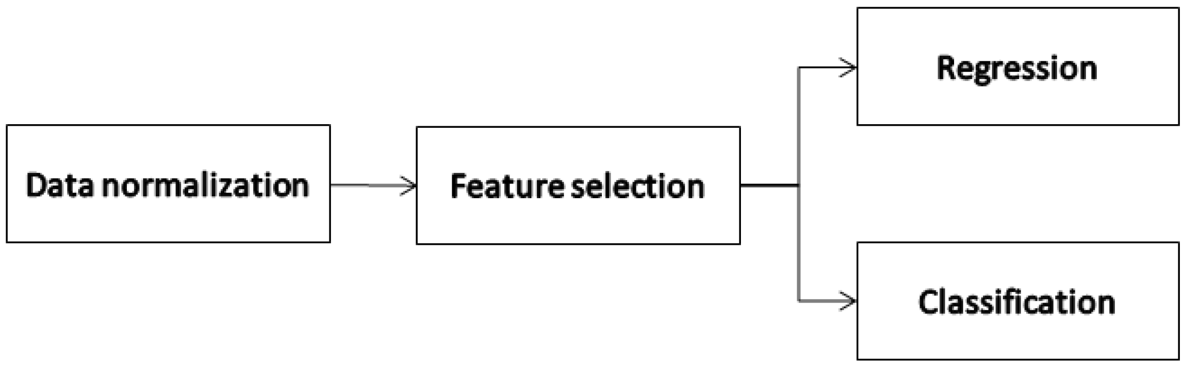
Figure 2.
Actual data vs estimated data for the best performing fold for the decision tree model - irrigated condition.
Figure 2.
Actual data vs estimated data for the best performing fold for the decision tree model - irrigated condition.
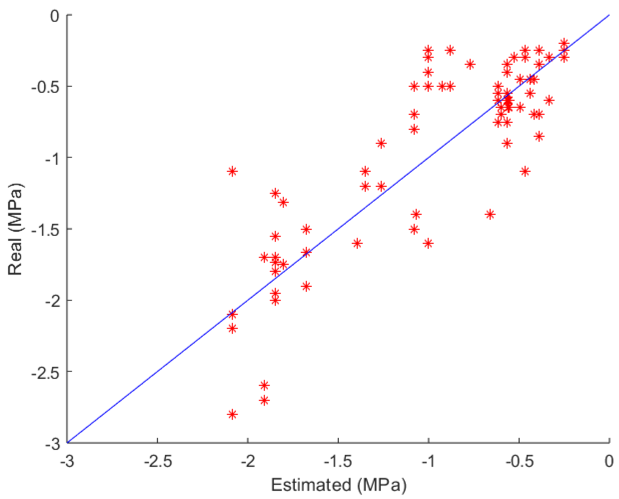
Figure 3.
Confusion matrix for the 5 most relevant features of fold 5, for the KNN classifier - Irrigated condition.
Figure 3.
Confusion matrix for the 5 most relevant features of fold 5, for the KNN classifier - Irrigated condition.
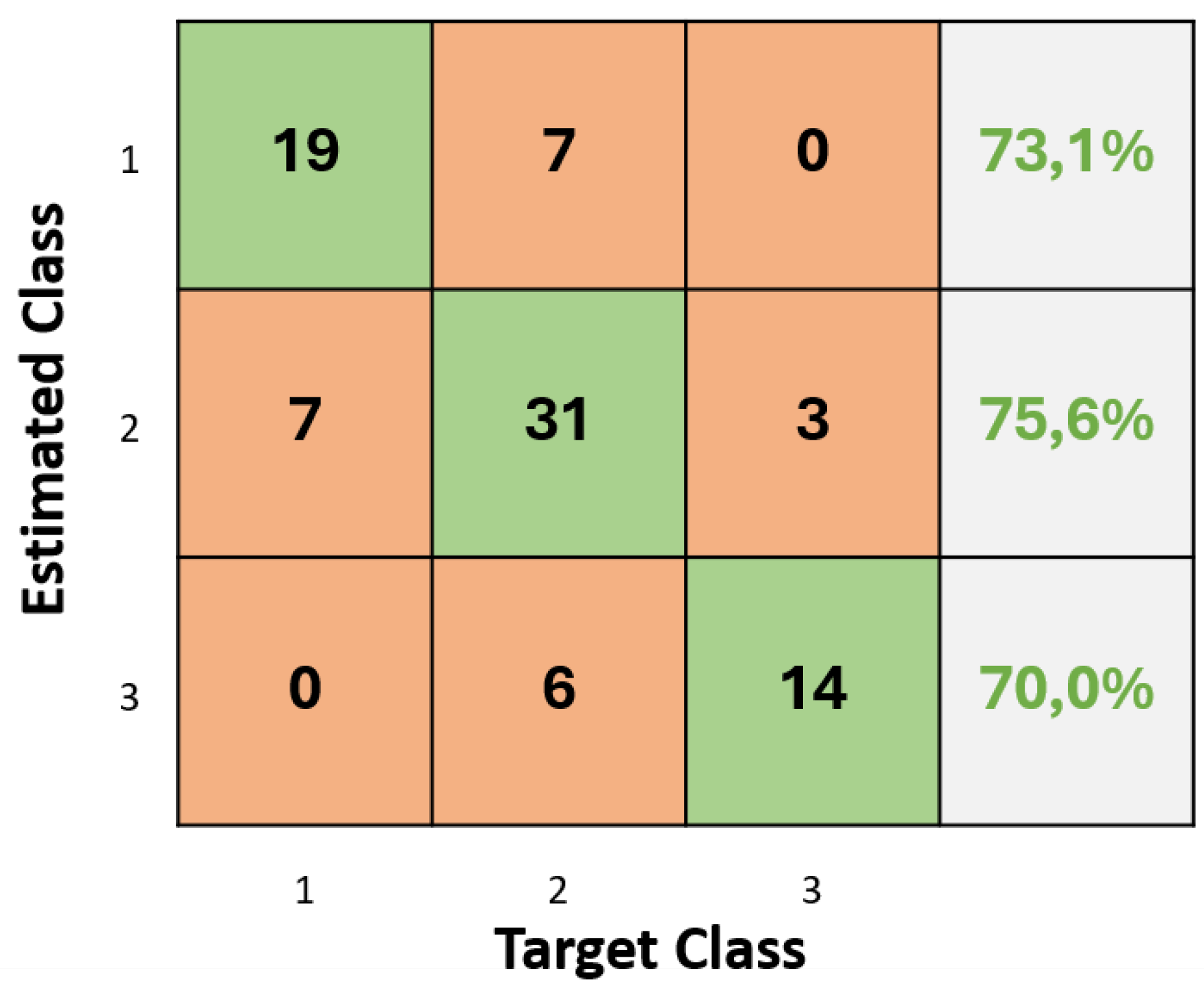
Figure 4.
Actual data vs estimated data for the best performing fold for the MLP model - rainfed condition.
Figure 4.
Actual data vs estimated data for the best performing fold for the MLP model - rainfed condition.
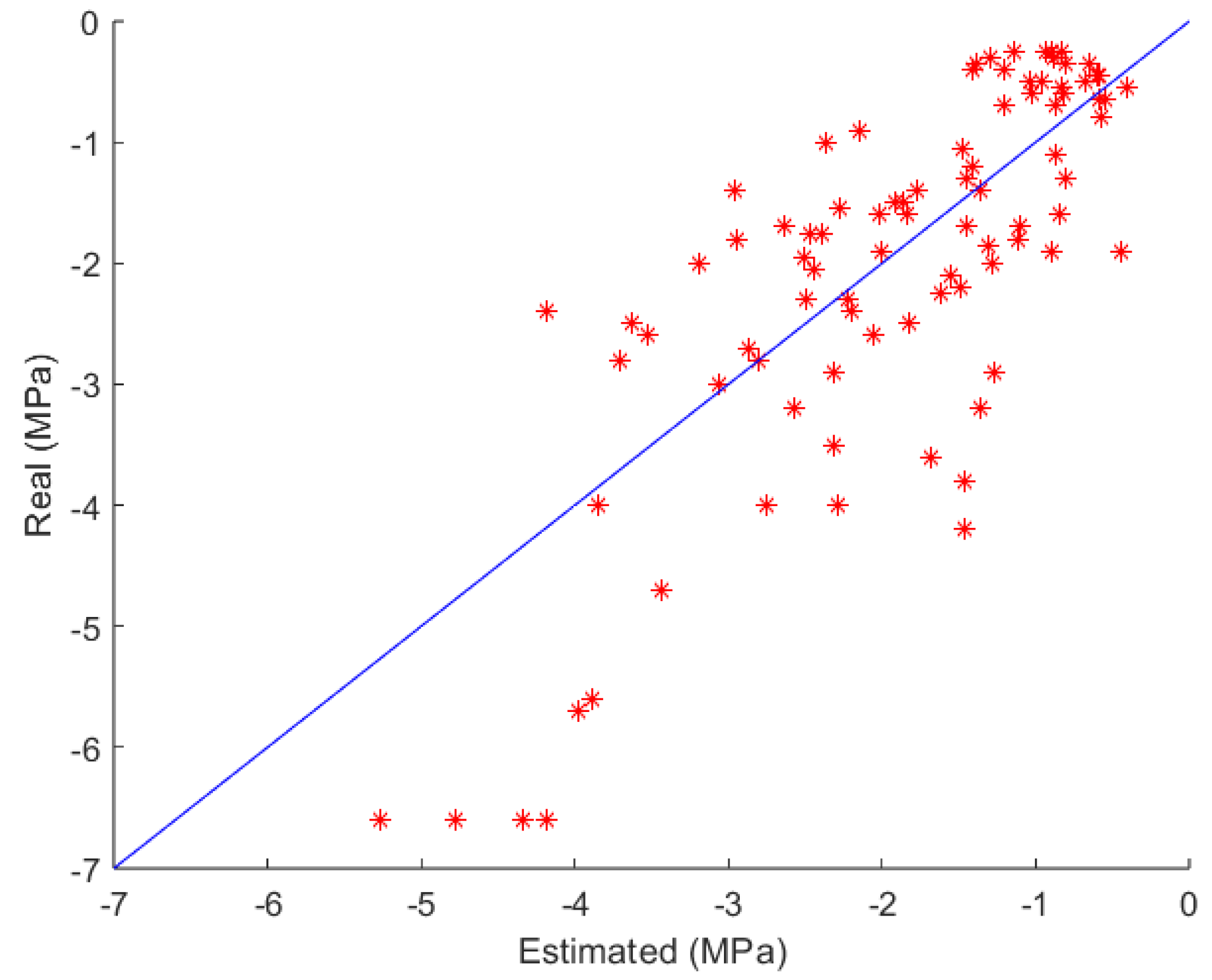
Figure 5.
Confusion matrix for the 20 most relevant features of fold 2, for the Random Forest classifier - rainfed condition.
Figure 5.
Confusion matrix for the 20 most relevant features of fold 2, for the Random Forest classifier - rainfed condition.
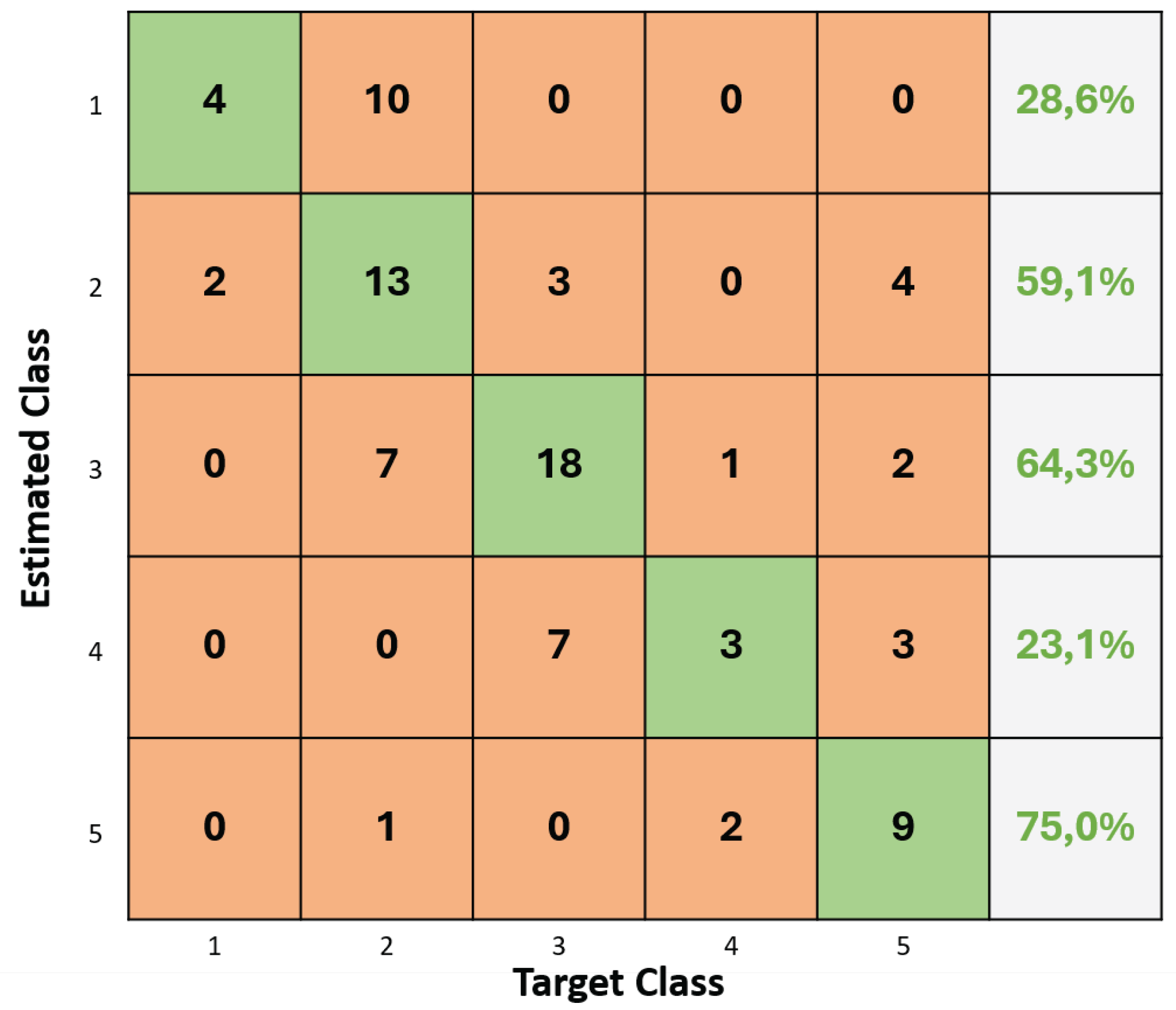

Table 1.
Interpretation of correlation coefficient values ().
| Value of | Interpretation |
|---|---|
| 0.00 to 0.19 | Very weak correlation |
| 0.20 to 0.39 | Weak correlation |
| 0.40 to 0.69 | Moderate correlation |
| 0.70 to 0.89 | Strong correlation |
| 0.90 to 1.00 | Very strong correlation |
Table 2.
Classes and ranges of water potential.
| Water Potential Values (W) (MPa) | Class |
|---|---|
| ΨW up to -0.5 MPa | 1 |
| ΨW between -0.5 and -1.4 MPa | 2 |
| ΨW between -1.5 and -2.4 MPa | 3 |
| ΨW between -2.5 and -3.5 MPa | 4 |
| ΨW less than -3.5 MPa | 5 |
Table 3.
Number of samples per class.
| Rainfed | Irrigated | |
|---|---|---|
| Class | Number of Samples | Number of Samples |
| 1 | 67 | 129 |
| 2 | 112 | 208 |
| 3 | 140 | 100 |
| 4 | 62 | - |
| 5 | 64 | - |
Table 4.
The 10 most relevant attributes for irrigated conditions.
| Ranking | Attribute Designation |
|---|---|
| 1 | Collection month |
| 2 | Reflectance for = 780nm |
| 3 | Reflectance for = 785nm |
| 4 | Collection year |
| 5 | Reflectance for = 783nm |
| 6 | Reflectance for = 781nm |
| 7 | Reflectance for = 779nm |
| 8 | Reflectance for = 784nm |
| 9 | Reflectance for = 782nm |
| 10 | Reflectance for = 779nm |
Table 5.
The 10 most relevant attributes for rainfed conditions.
| Ranking | Attribute Designation |
|---|---|
| 1 | Collection month |
| 2 | Reflectance for = 691nm |
| 3 | Reflectance for = 694nm |
| 4 | Reflectance for = 693nm |
| 5 | Reflectance for = 698nm |
| 6 | Reflectance for = 690nm |
| 7 | Reflectance for = 688nm |
| 8 | Reflectance for = 695nm |
| 9 | Reflectance for = 692nm |
| 10 | Reflectance for = 689nm |
Table 6.
Achieved RMSE and values for irrigated condition in terms of .
| 22 features | ||
|---|---|---|
| Method | ||
| MLP | 0.4189 ±0.0400 | 0.5733 ±0.0781 |
| Decision Tree | 0.4160 ±0.0284 | 0.5787 ±0.0684 |
| Random Forest | 0.4249 ±0.0363 | 0.5604 ±0.0687 |
| KNN | 0.4812 ±0.0373 | 0.4353 ±0.0788 |
| 10 features | ||
| Method | ||
| MLP | 0.4309 ±0.0487 | 0.5457 ±0.0933 |
| Decision Tree | 0.4063 ±0.0365 | 0.5965 ±0.0752 |
| Random Forest | 0.4325 ±0.0222 | 0.5482 ±0.0555 |
| KNN | 0.4605 ±0.0443 | 0.4867 ±0.0860 |
| 5 features | ||
| Method | ||
| MLP | 0.4205 ±0.0519 | 0.5697 ±0.0954 |
| Decision Tree | 0.3884 ±0.0299 | 0.6313 ±0.0569 |
| Random Forest | 0.4256 ±0.0449 | 0.5564 ±0.0837 |
| KNN | 0.4522 ±0.0324 | 0.5098 ±0.0663 |
Table 7.
Classification results in terms of balanced accuracy () for irrigated condition in %.
| Method | 22 features | 10 features | 5 features |
|---|---|---|---|
| MLP | 63.37 ±3.98 | 61.91 ±5.35 | 66.76 ±4.56 |
| Decision Tree | 64.39 ±1.36 | 65.39 ±5.26 | 64.59 ±2.61 |
| Random Forest | 64.40 ±2.51 | 66.99 ±4.58 | 65.60 ±4.83 |
| KNN | 66.76 ±6.50 | 66.77 ±5.52 | 67.73 ±3.48 |
Table 8.
Number of samples per class in the irrigated condition.
| Class | Training samples | Test samples |
|---|---|---|
| 1 | 103 | 26 |
| 2 | 167 | 41 |
| 3 | 80 | 20 |
Table 9.
Achieved RMSE and values for irrigated condition in terms of .
| 20 features | ||
|---|---|---|
| Method | ||
| MLP | 1.0569±0.1246 | 0.5441±0.1099 |
| Decision Tree | 1.0959±0.1334 | 0.5169±0.1153 |
| Random Forest | 1.0982±0.1196 | 0.5117±0.1045 |
| KNN | 1.1476±0.1197 | 0.4728±0.0952 |
| 10 features | ||
| Method | ||
| MLP | 1.0887±0.1423 | 0.5129±0.1101 |
| Decision Tree | 1.0938±0.1399 | 0.5141±0.1216 |
| Random Forest | 1.1361±0.1287 | 0.4783±0.0999 |
| KNN | 1.1577±0.1255 | 0.4725±0.0913 |
| 5 features | ||
| Method | ||
| MLP | 1.1160±0.1157 | 0.4917±0.1061 |
| Decision Tree | 1.0840±0.1388 | 0.5250±0.1182 |
| Random Forest | 1.0927±0.1126 | 0.5173±0.0930 |
| KNN | 1.1229±0.1278 | 0.5018±0.0946 |
Table 10.
Classification results in terms of balanced accuracy () for rainfed condition in %.
| Method | 20 features | 10 features | 5 features |
|---|---|---|---|
| MLP | 45.38±5.84 | 45.69±4.99 | 45.86±2.46 |
| Decision Tree | 46.17±3.49 | 46.59±1.26 | 43.94±3.53 |
| Random Forest | 47.55±2.41 | 46.10±1.92 | 46.17±4.57 |
| KNN | 43.14±2.95 | 46.65±4.90 | 42.72±3.67 |
Table 11.
Number of samples per class in the rainfed condition.
| Class | Training samples | Test samples |
|---|---|---|
| 1 | 53 | 14 |
| 2 | 90 | 22 |
| 3 | 112 | 28 |
| 4 | 49 | 13 |
| 5 | 52 | 12 |
Disclaimer/Publisher’s Note: The statements, opinions and data contained in all publications are solely those of the individual author(s) and contributor(s) and not of MDPI and/or the editor(s). MDPI and/or the editor(s) disclaim responsibility for any injury to people or property resulting from any ideas, methods, instructions or products referred to in the content. |
© 2025 by the authors. Licensee MDPI, Basel, Switzerland. This article is an open access article distributed under the terms and conditions of the Creative Commons Attribution (CC BY) license (http://creativecommons.org/licenses/by/4.0/).
Copyright: This open access article is published under a Creative Commons CC BY 4.0 license, which permit the free download, distribution, and reuse, provided that the author and preprint are cited in any reuse.


