Submitted:
13 July 2025
Posted:
15 July 2025
You are already at the latest version
Abstract
We investigate binary sequences generated by non-Markovian rules with memory length $\mu$, similar to those adopted in Elementary Cellular Automata. This generation procedure is equivalente to a shift register and certain rules produce sequences with maximal periods, known as de Bruijn sequences. We introduce a novel methodology for generating de Bruijn sequences that combines: (i) a set of derived properties that significantly reduce the space of feasible generating rules, and (ii) a neural network-based classifier that identifies which rules produce de Bruijn sequences. Experiments for large values of $\mu$ demonstrate the approach’s effectiveness and computational efficiency.
Keywords:
sequence generation
; cellular automata with memory
; de bruijn sequences
; feasible rule reduction
; neural network
1. Introduction
Cellular Automata (CA) are a class of dynamical systems that evolve in discrete time and space [17,18]. A CA consists of cells (or agents), each of which can adopt a state from a discrete set. The most commonly used alphabet is binary, typically denoted by . The CA evolves by applying generating rules at each time step. These rules can be static or dynamic (i.e., they may change depending on the current state of the entire CA), and either local or global, depending on whether they involve only neighboring cells or the entire population.
From an initial configuration, the state of the CA evolves over time according to the specified rules. The update rule for each cell can depend on both the past states of the cell itself (temporal dimension) and the states of its neighboring cells (spatial dimension). Elementary one-dimensional cellular automata (1dCA) typically assume a memoryless structure with a linear topology, where each cell interacts only with its nearest neighbors [17]. More complex models incorporate memory—i.e., dependence on a set of past states—and long-range spatial influences [13,15].
Relatively less attention has been given to zero-dimensional cellular automata (0dCA), which consist of a single cell whose state is updated based solely on its own past states. Despite their apparent simplicity, 0dCA do not involve interactions between multiple cells, their time evolution yields interesting sequences of symbolic states. The rules governing such systems depend on the memory —the number of previous states influencing the next state—and the alphabet , the number of possible states a cell can take. Generally, the complexity of the system increases with both and . For simplicity, we focus on binary systems, i.e., , using the symbols .
2. 0-Dimensional CA
Symbolic sequences naturally arise in discrete dynamical systems, e.g., CA [11]. From an initial condition, the next state is computed according to a generation rule (or function) that depends on previous states. For instance, a classical non-Markovian binary time series can be defined by initial values and , and a recursive rule:
With initial states and , the sequence continues as , , , , etc., producing the binary sequence:
This sequence is clearly periodic with period . In this case, the next digit depends on the two previous digits, implying a memory .
Other examples with can be constructed using logical operators. For instance, applying the AND function with the rules:
to the initial pair produces the sequence:
Similarly, applying the OR function:
to the same initial configuration results in:
Both sequences converge to fixed values (0 or 1), i.e., their periods are , and these fixed points are independent of the initial configuration.
In contrast, applying the XOR function:
to the initial state yields:
with period . However, using the same rule with the initial configuration: results in a constant sequence for all . These examples illustrate that the resulting behavior depends not only on the rule but also on the initial conditions.
For any finite memory , all sequences generated in this framework are eventually periodic. That is, for any rule and initial condition, the sequence will eventually settle into a repeating pattern (also referred to as a motif or loop). The maximum possible period for a sequence with memory is:
As increases, the sequences may resemble aperiodic ones, making them useful for computing pseudorandom numbers to be applied in Monte Carlo simulations, and cryptographic systems [7]. Truly aperiodic behavior can only arise when , or when the alphabet is infinite (e.g., using real-valued states).
To explore periodicity in 0dCA, we adopt combinatorial generating rules analogous to those used in 1dCA [17], with memory playing the role of spatial interaction. Formally, a generating rule with memory is a function that maps each of the binary sequences of length to a single binary output:
where for all i (see Figure 1). Starting from an initial configuration, the rule is applied recursively to generate the digits of the sequence as follows:
which eventually converges to an asymptotic pattern with period T.
For example, when , there are possible rules—corresponding to Wolfram’s elementary 1dCA rules. Figure 1A shows the XOR rule for , represented by the binary rule string 10010110, which corresponds to rule number 150 in Wolfram’s classification. Applying this rule to the initial configuration yields:
which has period .
In general, for a given , the total number of possible generating rules is , and the maximum number of binary sequences generated from these rules is:
This number grows super-exponentially with , making exhaustive analysis computationally infeasible for large . For instance, when , there are approximately rules, each of which must be applied to 1024 different initial configurations.
This raises the fundamental question: given a memory value and an initial configuration, is it possible to predict the asymptotic pattern and period T of the resulting sequence? While this is tractable for small via exhaustive enumeration, alternative methods are necessary for large due to the sheer size of the rule space.
It is worth noting that the 0-dimensional Cellular Automata (0dCA) with memory, as defined above, are equivalent to sequences generated by a Linear Feedback Shift Register (LFSR). This type of sequence has been extensively studied, and a vast body of literature exists on the subject [9]. In particular, significant attention has been devoted to the characterization and computation of shift register sequences with maximum period—commonly known as de Bruijn sequences [5,8,14]. As we will show in the next section, there exists a one-to-one correspondence between de Bruijn sequences and their generating rules, which we will refer to as de Bruijn rules.
3. Rules that Generate Maximum Period Sequences: de Bruijn Rules
For a given memory length , the maximum period that a generated binary sequence can attain is . Naturally, the minimum period is 1, corresponding to sequences that converge to fixed points (e.g., either 0 or 1). For small values of , it is feasible to generate all possible sequences and compute their corresponding periods. Figure 2 and Table 1 show, respectively, the bar chart of the observed periods and the associated frequencies for the case .
Sequences with maximum period, known as de Bruijn sequences, are of particular interest. These are cyclic sequences of length in which every possible binary substring of length appears exactly once. For small values of , it is straightforward to generate all possible de Bruijn sequences. There exists a unique de Bruijn sequence for , namely 0011. For , there are two such sequences: 00010111 and 00011101, that are generated by rules 45 and 75, respectively (rule 45 is graphically described in Figure 1B).
Since these sequences are cyclic, their representations are not unique; by convention, we select the lexicographically least sequence (i.e., the smallest in binary order and decimal number) as the representative of the equivalence class. Specially significative is the lexicographically least sequence for each memory , that is referred to as the granddaddy in [12].
The number of binary de Bruijn sequences for a given is given by [2,5]. This number grows also superexponentially with and reaches extremely large values even for moderate . For example, for , . Generating all de Bruijn sequences is a challenging combinatorial problem that remains unsolved in full generality, though various efficient construction algorithms have been proposed (see, for instance, [6]).
De Bruijn sequences can be generated by applying certain specific rules, independently of the initial configuration of length . In other words, there exists a bijection between de Bruijn sequences and their corresponding rules, which we refer to as de Bruijn rules . Table 2 lists the de Bruijn rules and their de Bruijn sequences for , and 4, expressed both as binary maps and in their corresponding decimal representations.
For , there are de Bruijn rules and their associated de Bruijn sequences. As it can be seen, the granddaddy sequence is: 0000100110101111. The corresponding granddaddy rule is 3825, with binary representation 0000111011110001. For , the number of de Bruijn sequences is . The granddaddy rule in this case is 00001100111111101111001100000001 (whose decimal representation is 218034945), which generates the granddaddy sequence: 00000100011001011011101010011111.
4. Characterization of de Bruijn Rules
As stated in the previous section, certain generating rules produce sequences with maximum period—we refer to them as de Bruijn sequences. Therefore, a complete characterization of such rules emerges as a fundamental goal. The following properties help identify and constrain the set of de Bruijn rules, and can be used to systematically search for them:
- Boundary Conditions: The binary representations of de Bruijn rules must start with 0 and end with 1. This condition arises from the convention in rule ordering, which arranges input strings from the highest binary value () to the lowest (), and from the necessity to avoid fixed points (e.g., if , the sequence remains constant). This constraint immediately reduces the number of candidate rules by a factor of 4. For example, for , the number of potentially valid rules is reduced from to 16384.
-
Symmetry and Parity: The binary representations of de Bruijn rules are symmetric with respect to their midpoint, such that each half is the complement of the other. This symmetry ensures parity: the number of 0s equals the number of 1s, although the balance may be broken within each half. Under this constraint, valid de Bruijn rules correspond to multiples of certain numbers derived from sequences of Evil Odd numbers [1], multiplied by factors denoted as .For instance, if we denote the Evil Odd Numbers, i.e., an odd number whose binary representation contains an even number of 1, for each as , being , we get:The factors follow the recursive relation:For instance, , , , and . Table 2 presents all de Bruijn rules for whose decimal representations are products of an Evil Odd number and the corresponding . Note, however, that not all Evil Odd numbers yield valid de Bruijn rules, and the problem of determining which ones do remains open for larger values of . For , applying these conditions reduce the feasible set of de Bruijn rules to 32.
-
Constrained Position Pairs: There exist pairs of positions in the binary representation of de Bruijn rules that cannot simultaneously take the same value (1 for even -values and 0 for odd ones). This condition is applied only to the first half of the binary string for symmetry (according to the previous item) and depends on according to a recursive pattern. Specifically: For , the constrained positions are and , and
- -
- If , then and .
- -
- If , then and ,
for . This structural condition eliminates of the remaining candidates. For example, for these positions are and . For , and .Remarkably, for , the final count of feasible de Bruijn rules after applying all constraints is 24. In general, for all values of , the feasible set exceeds the actual number of de Bruijn rules (see Table 3). -
Symmetric Rule Invariance: If a rule of the form:is a de Bruijn rule, then its mirrored version:is also a de Bruijn rule.This property reflects the inherent symmetry and reversibility in de Bruijn rule structure. It ensures that for each valid de Bruijn rule constructed in this way, a corresponding reverse-complement rule also exists within the de Bruijn set.
The application of the properties stated in the previous paragraphs to the entire set of generating rules significantly reduces the number of feasible rules that can yield de Bruijn sequences. Table 3 presents the total number of rules, the number of de Bruijn sequences, the number of feasible rules after applying the constraints, and the corresponding ratios.
As can be observed, the number of feasible rules that need to be checked to find de Bruijn rules is drastically smaller than the total number of rules for each value. For instance, when , the reduction factor is approximately . In the same case, the ratio between the number of rules that actually yield de Bruijn sequences and the number of feasible rules is around . For such low values of , a brute-force approach may still be used to generate all de Bruijn sequences. However, a more efficient and structured methodology will be presented in the next section.
5. Neural Networks to Classify de Bruijn Rules
An alternative approach to identifying de Bruijn rules is to apply machine learning methods. In particular, neural networks are especially well-suited for classification tasks [4]. In this section, we present a neural network model for classifying the feasible rules into two categories: de Bruijn rules (coded by 1) and the rest (0). Although classification based on the sequence period is also possible, it would require accounting for dependence on initial conditions. The classification is performed for and (see Table 4).
We implemented a binary classification model using a feedforward neural network in R [16]. The analysis followed these main steps:
- Data loading and preprocessing: The input data consisted of a character string representing a binary sequence and a binary integer label.
- Feature extraction: Each rule was split into individual bits transforming the strings into a matrix where each column corresponds to a bit ( to bit). According to the necessary properties of de Bruijn rules (see Section 4), only the first bits were retained for further analysis. The first and the bits were also removed because they are necessarily 0.
- Dataset splitting: The data was randomly split into training (80%) and testing (20%) subsets to evaluate model performance on unseen data.
Feedforward neural networks are highly suitable for structured, tabular data, such as the bit vectors extracted from rule representations. They can capture complex, non-linear relationships between input features without requiring explicit feature engineering. In our case, the binary inputs represent discrete features, and their interactions are not trivially captured by simpler linear models. The multi-layer architecture enables hierarchical feature learning, significantly improving classification accuracy.
For the case , the neural network architecture includes:
- An input layer with 14 features (bits),
- A hidden dense layer with 32 units and ReLU activation,
- A second hidden dense layer with 16 units and ReLU activation,
- An output layer with 1 unit and sigmoid activation for binary classification.
The model was compiled using the Adam optimizer (learning rate ), binary cross-entropy loss function, and accuracy as a performance metric. The dataset includes the complete set of 6144 feasible rules, one-third of which are de Bruijn rules (see Table 3). Training was performed over 100 epochs with a batch size of 4. Model evaluation was conducted on the test set by calculating accuracy, sensitivity, and specificity (see Table 4). Class labels were assigned using a threshold of 0.5 on the predicted probabilities. The resulting classifier achieved outstanding performance, with an accuracy exceeding 99% for .
The more challenging case of involves a rule space of size on the order of , with approximately 67 million de Bruijn rules (see Table 3). As a matter of fact, we can only use a sample of the total rule space that is randomly analyzed and classified into the two classes.
Optimal results were achieved using a slightly deeper neural network with the following architecture:
- Three hidden dense layers with 64, 64, and 8 units respectively,
- ReLU activations in all hidden layers,
- A sigmoid output unit for binary classification.
Training used a batch size of 64 and a learning rate of . The dataset consists of a sample of feasible rules, half of which are de Bruijn rules. As before, 80% of the dataset was used for training, and the remainder for testing. A threshold of 0.5 was again applied to the output probabilities to assign class labels. As shown in Table 4, this model also demonstrated excellent classification metrics.
Once the neural network model is available, any given rule can be evaluated to determine, with high probability, whether it is a de Bruijn rule. If the prediction is positive, the rule is then applied to generate the corresponding binary sequence, which must ultimately be verified to confirm that it satisfies the de Bruijn sequence properties.
6. Discussion
The successive application of updating rules to an initial configuration of generates a binary sequence that becomes asymptotically periodic. The size of the initial configuration depends on the memory of the rule, denoted by , which is the number of digits required to update the next one. For large values of , the number of possible generating rules becomes so large that an exhaustive analysis of the resulting patterns is infeasible. Particularly relevant is a specific and highly constrained subset of rules, that we named as de Bruijn rules, that generate sequences of maximum period, known as de Bruijn sequences. Although these sequences represent only a tiny fraction of the entire set of possible sequences, their sheer number for large remains enormous, and the complete and effective generation of all such sequences is still an open problem.
In this paper, we have presented a novel approach to compute de Bruijn sequences that combines two complementary methodologies. First, by exploiting structural properties of de Bruijn rules—i.e., those rules that generate maximum period sequences—a drastic reduction of the full set of candidate rules can be achieved. Table 3 summarizes the reduction ratios for several values of . Second, we applied a machine learning approach to this feasible subset in order to accurately identify the de Bruijn rules. As shown in Section 5, the use of a classical neural network model for , and 6 allows for nearly complete classification of de Bruijn rules in the smaller cases, and achieves over 99% and 94% accuracy for and , respectively. Once the de Bruijn rules are identified, the corresponding de Bruijn sequences are straightforward to construct. This would allow to find granddaddy sequence that represents the lexicographically smallest member for each -value.
To the best of our knowledge, this is the first attempt to generate de Bruijn sequences using a hybrid approach that integrates Machine Learning techniques within the framework of Cellular Automata for generating maximum period sequences. It is worth mentioning that existing methods based on Feedback Shift Register generation have not definitively solved the problem. Therefore, we believe that the results presented in this paper represent a significant step forward in the study and generation of this important class of sequences.
Author Contributions
F. J. M and J. C. N contributed equally to this manuscript.
Funding
This research received no external funding.
Data Availability Statement
The data presented in this study are available on request from the corresponding author.
Conflicts of Interest
The authors declare no conflicts of interest.
References
- OEIS Foundation Inc. A129771 in the On-Line Encyclopaedia of Integer Sequences. Available online: https://oeis.org/A129771 (accessed on 10 July 2025).
- OEIS Foundation Inc. A016031 in the On-Line Encyclopaedia of Integer Sequences. Available online: https://oeis.org/A016031 (accessed on 10 July 2025).
- Allaire, J. , Chollet, F., et al. (2024). keras: R Interface to ’Keras’. R package version 2.16.0. URL: https://CRAN.R-project.org/package=keras.
- Bishop, C.M. (1995). Neural Networks for Pattern Recognition. Oxford University Press.
- De Bruijn, G. (1946) A combinatorial problem, Nederl. Akad. Wetensch. Proc., 49, 758-764.
- De Bruijn Sequence and Universal Cycle Constructions (2024). Available online: http://debruijnsequence.org. (accessed on 10 July 2025).
- Etzion, T. Sequences and the de Bruijn Graph: Properties, Constructions, and Applications. Elsevier (2024).
- Fredricksen, H. (1982) A Survey of Full Length Nonlinear Shift Register Cycle Algorithms. SIAM Review, Vol. 24, No. 2, pp. 195-221.
- Golomb, W. (1967) Shift Register Sequences, Holden-Day, San Francisco, 1967, pp. 118-122.
- Hall, M. (1967) Combinatorial Theory, Blaisdell, Waltham, MA.
- Jin, W. and Chen, F. (2025). Symbolic Dynamics of Cellular Automata. In book: Advances in Cellular Automata (pp.375-397). [CrossRef]
- Knuth, D.E. The art of computer programming, volume 4A: combinatorial algorithms, part 1. Pearson Education (2011).
- Li, W. (1992) Phenomenology of Noniocal Cellular Automata. J. Stat. Phys. Vol. 68, Nos. 5/6.
- Ralston, A. (1982) De Bruijn Sequences: A Model Example of the Interaction of Discrete Mathematics and Computer Science. Mathematics Magazine, Vol. 55, No. 3, pp. 131-143.
- Alonso-Sanz, R. Discrete systems with memory, World Scientific Series on Nonlinear Science Series A: Volume 75 (2011).
- R Core Team (2024). R: A language and environment for statistical computing. R Foundation for Statistical Computing, Vienna, Austria. URL: https://www.R-project.org/.
- Wolfram, S. (1983) Statistical mechanics of cellular automata. Reviews of Modern Physics, Vol. 55, No. 3, 601-644.
- Wolfram, S. (1984) Computation Theory of Cellular Automata. Commun. Math. Phys. 96, 15- 57.
Figure 1.
Two generating rules with memory . A) Rule 150, whose binary representation is 10010110. This corresponds to the following assignments for each 3-tuple (ordered from 111 to 000): , , , , , , , . The application of this rule to four different initial triplets is shown on the left. As observed, the resulting sequences are periodic with periods 1, 4, 1, and 2 (from top to bottom). The dynamics of this rule can be visualized as a directed graph, shown at the bottom. Each node represents a possible 3-tuple; a directed edge from node x to node y exists if applying the rule to x yields the last digit of y. This graph is not connected and does not contain a Hamiltonian path. B) Rule 45, with binary representation 00101101, corresponds to the truth table shown on the left of panel B. In contrast to Rule 150, applying Rule 45 to any of the initial triplets yields the same cyclic sequence of maximum period , namely, the de Bruijn sequence . This rule is thus a de Bruijn rule. The associated graph, built as described above, is a de Bruijn graph because it contains a Hamiltonian path through all nodes.
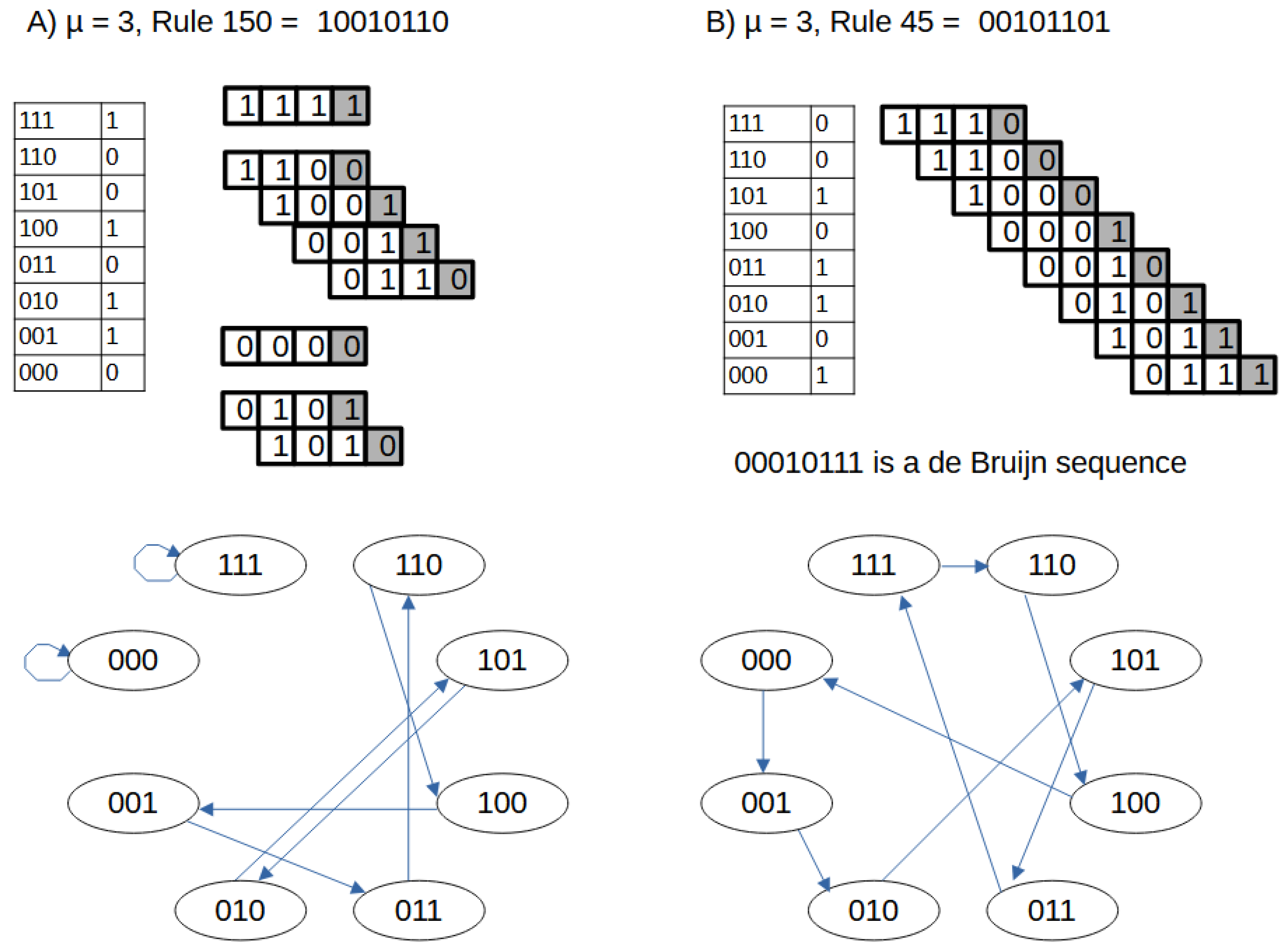
Figure 2.
Bar chart of periods for a memory . The frequencies correspond to the values presented in Table 1. Similar bar charts appear for other -values. Note that the maximun period has the lower occurrence; as a matter of fact, there are de Bruijn sequences.
Figure 2.
Bar chart of periods for a memory . The frequencies correspond to the values presented in Table 1. Similar bar charts appear for other -values. Note that the maximun period has the lower occurrence; as a matter of fact, there are de Bruijn sequences.
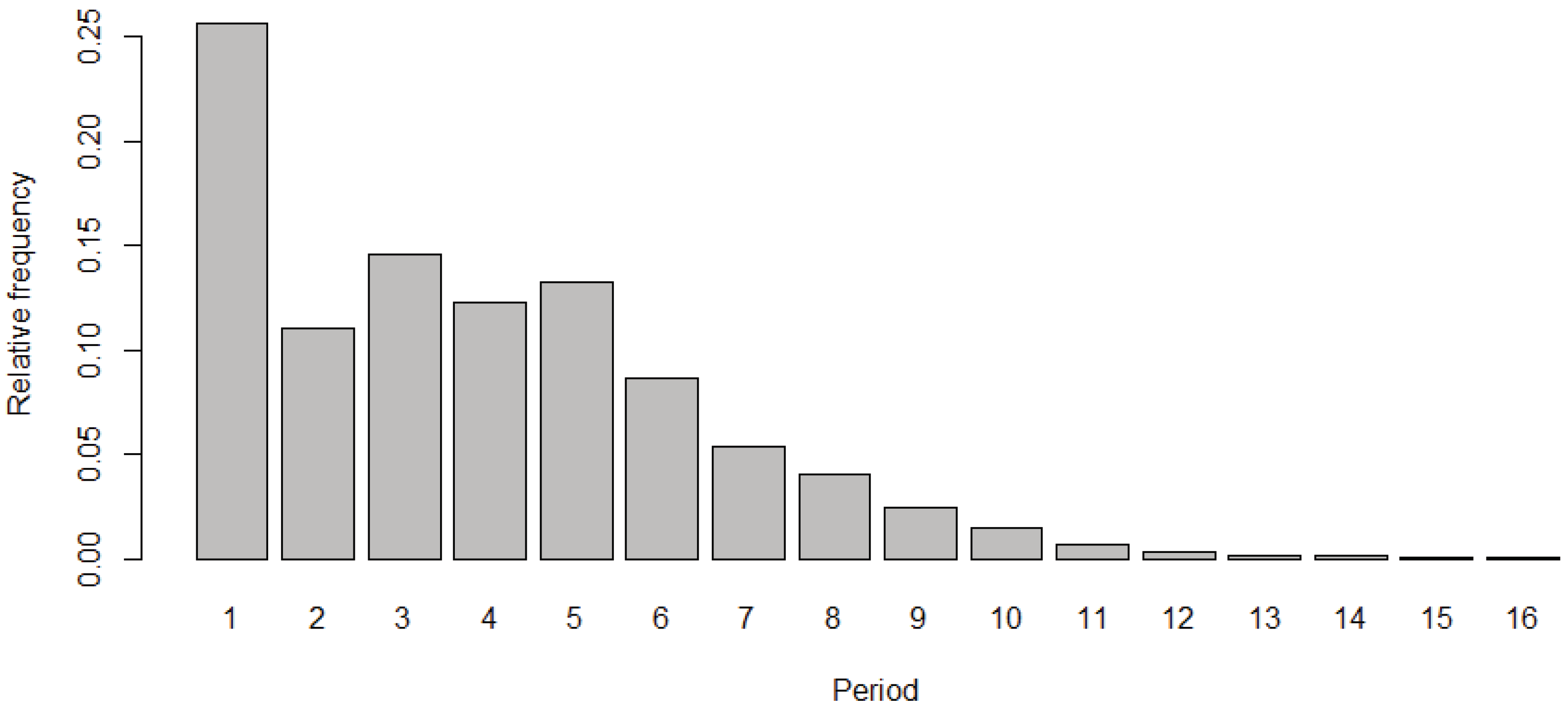

Table 1.
Number of rules that generates sequences with each of the possible periods that can appear, from 1 to 16, for . The bar chart exhibits three peaks at , and . For the distribution decreases monotonously (see Figure 2)
Table 1.
Number of rules that generates sequences with each of the possible periods that can appear, from 1 to 16, for . The bar chart exhibits three peaks at , and . For the distribution decreases monotonously (see Figure 2)
| 1 | 2 | 3 | 4 | 5 | 6 | 7 | 8 | 9 | 10 | 11 | 12 | 13 | 14 | 15 | 16 |
|---|---|---|---|---|---|---|---|---|---|---|---|---|---|---|---|
| 16784 | 7220 | 9547 | 8060 | 8665 | 5668 | 3494 | 2670 | 1592 | 977 | 421 | 192 | 90 | 77 | 63 | 16 |
Table 2.
Correspondence betweeen de Bruijn rules and de Bruijn sequences for and 4. It is also shown the Evil Odd Number that divides each de Bruijn rule, leaving the remainder .
Table 2.
Correspondence betweeen de Bruijn rules and de Bruijn sequences for and 4. It is also shown the Evil Odd Number that divides each de Bruijn rule, leaving the remainder .
| Evil odd number | Rule in decimal | Rule in binary | de Bruijn Sequence | ||
|---|---|---|---|---|---|
| 1 | - | - | 1 | 01 | 01 |
| 2 | 3 | 1 | 3 | 0011 | 0011 |
| 3 | 3 | 15 | 45 | 00101101 | 00010111 |
| 3 | 5 | 15 | 75 | 01001011 | 00011101 |
| 4 | 3 | 255 | 765 | 0000001011111101 | 0000101101001111 |
| 4 | 9 | 255 | 2295 | 0000100011110111 | 0000110100101111 |
| 4 | 15 | 255 | 3825 | 0000111011110001 | 0000100110101111 |
| 4 | 17 | 255 | 4335 | 0001000011101111 | 0000111100101101 |
| 4 | 27 | 255 | 6885 | 0001101011100101 | 0000101111001101 |
| 4 | 29 | 255 | 7395 | 0001110011100011 | 0000110101111001 |
| 4 | 43 | 255 | 10965 | 0010101011010101 | 0000101001101111 |
| 4 | 57 | 255 | 14535 | 0011100011000111 | 0000110111100101 |
| 4 | 65 | 255 | 16575 | 0100000010111111 | 0000111101001011 |
| 4 | 71 | 255 | 18105 | 0100011010111001 | 0000100111101011 |
| 4 | 75 | 255 | 19125 | 0100101010110101 | 0000101111010011 |
| 4 | 83 | 255 | 21165 | 0101001010101101 | 0000101100111101 |
| 4 | 85 | 255 | 21675 | 0101010010101011 | 0000111101011001 |
| 4 | 89 | 255 | 22695 | 0101100010100111 | 0000110010111101 |
| 4 | 99 | 255 | 25245 | 0110001010011101 | 0000101001111011 |
| 4 | 113 | 255 | 28815 | 0111000010001111 | 0000111101100101 |
Table 3.
Table resulting from the application of the properties described in Section 4. The second column, , indicates the total number of rules for each value of . The third column shows the number of feasible rules remaining after applying the constraints detailed in Section 4. The fourth column lists the number of de Bruijn rules. The remaining columns present ratios between these subsets. Particularly noteworthy is the fifth column, which displays the ratio between the feasible subset and the total number of rules. As increases, the reduction in the search space for de Bruijn rules becomes dramatic — for example, for , the feasible subset constitutes only about of the full rule set.
| # Feasible | # de Bruijn | Feasible/Total | de Bruijn/Total | de Bruijn/Feasible | ||
|---|---|---|---|---|---|---|
| 2 | 16 | 1 | 0.0625 | |||
| 3 | 256 | 2 | 2 | 0.0078125 | 0.0078125 | 1 |
| 4 | 65536 | 24 | 16 | 0.000366211 | 0.000244141 | 0.66666667 |
| 5 | 4294967296 | 6144 | 2048 | 1.4305E-06 | 4.7683E-07 | 0.33333333 |
| 6 | 1.84467E+19 | 402653184 | 67108864 | 2.1827E-11 | 3.6379E-12 | 0.16666667 |
| 7 | 3.40282E+38 | 1.7293E+18 | 1.4411E+17 | 5.082E-21 | 4.2351E-22 | 0.08333333 |
| 8 | 1.15792E+77 | 3.1901E+37 | 1.3292E+36 | 2.7550E-40 | 1.1479E-41 | 0.04166667 |
| 9 | 1.3408E+154 | 1.0855E+76 | 2.2615E+74 | 8.0964E-79 | 1.6867E-80 | 0.02083333 |
Table 4.
Evaluation metrics for the neural network models applied to classify the de Bruijn rules for memories with and . Total refers to the sum: , and corresponds to one fith of the whole data set. Positive class considered: 1→ de Bruijn.
Table 4.
Evaluation metrics for the neural network models applied to classify the de Bruijn rules for memories with and . Total refers to the sum: , and corresponds to one fith of the whole data set. Positive class considered: 1→ de Bruijn.
| Metric (definition) | ||
|---|---|---|
| True Positives (TP) | 397 | 198563 |
| False Positives (FP) | 3 | 19839 |
| True Negatives (TN) | 820 | 180668 |
| False Negatives (FN) | 9 | 930 |
| Accuracy, (TP + TN) / Total | 0.9902 | 0.9481 |
| Sensitivity (Recall), TP / (TP + FN) | 0.9780 | 0.9953 |
| Specificity, TN / (TN + FP) | 0.9964 | 0.9011 |
| Precision (PPV), TP / (TP + FP) | 0.9925 | 0.9092 |
| Negative Predictive Value (NPV), TN / (TN + FN) | 0.9891 | 0.9949 |
| Balanced Accuracy, (Sens. + Spec.) / 2 | 0.9872 | 0.9482 |
| Detection Rate, TP / Total | 0.3230 | 0.4976 |
| Detection Prevalence, (TP + FP) / Total | 0.3255 | 0.5473 |
| True Prevalence, (TP + FN) / Total | 0.3304 | 0.4999 |
Disclaimer/Publisher’s Note: The statements, opinions and data contained in all publications are solely those of the individual author(s) and contributor(s) and not of MDPI and/or the editor(s). MDPI and/or the editor(s) disclaim responsibility for any injury to people or property resulting from any ideas, methods, instructions or products referred to in the content. |
© 2025 by the authors. Licensee MDPI, Basel, Switzerland. This article is an open access article distributed under the terms and conditions of the Creative Commons Attribution (CC BY) license (http://creativecommons.org/licenses/by/4.0/).
Copyright: This open access article is published under a Creative Commons CC BY 4.0 license, which permit the free download, distribution, and reuse, provided that the author and preprint are cited in any reuse.


