Submitted:
12 July 2025
Posted:
15 July 2025
Read the latest preprint version here
Abstract
Landslides pose a significant hazard to human activities, often causing substantial damage to human lives and infrastructure. Countermeasures are measures taken to prevent or mitigate the effects of landslides. To implement suitable structural countermeasures, the type of landslide is essential. This study aims to develop a model for earthquake-unaffected regions to identify cliff-type landslides from a landslide inventory where the type is not specified . The model utilizes Forest-based and Boosted Classification and Regression tools within ArcGIS Pro software.21 LCF and 167 LS points and 167 non-LS points were used to train the model referring Tokushima Prefecture. Trained Model demonstrated an accuracy of 0.84, a sensitivity of 0.84, MCC of 0.68, F1 score of 0.84, a mean of 0.80, a median of 0.80 and a standard deviation of 0.03. This is a good indication of the model's overall the reliability. Predictions were made to Kegalle district in Sri Lanka. Validation was made referring the recently modified inventory incidents with landslide type, which showed 80.1% matched accurately. Model was used to predict cliff type LS in the inventory before modifying in KD. This model aid in identifying cliff-type landslides from inventories and to prevent future occurrences in applying appropriate countermeasures.
Keywords:
Cliff Type
; Landslide (LS)
; Inventory
; Landslide Conditioning Factors (LCF)
; Forest-based and Boosted Classification and Regression tool (FBCR) Model
; Tokushima Prefecture (TP) Kegalle District (KD)
1. Introduction
Landslides are defined as mass movements of soil and rocks along a slope. Landslides occur when slopes undergo a decrease in the shear strength of the hillside material due to an increase in the shear stress [33].The global statistics on landslide damage revealed that there were more than 3876 landslides from 1995 to 2014, in which 11,689 injuries and 163,658 deaths were reported. Research findings recorded that only in the year 2014, about 174 landslides occurred worldwide resulting in devastating consequences on human as well as natural resources [2].
Large parts of the United Kingdom experienced several months of above-average precipitation from April to December 2012 making it one of the wettest periods of time for the country since meteorological records began. Throughout this period and into early 2013, a marked increase in the number of landslides was widely reported and captured in the National Landslide Database (NLD) of the British Geological Survey (BGS) [38].
27 European countries over the last 20 years (1995–2014), a total of 1370 deaths and 784 injuries were reported resulting from 476 landslides. In some countries, these landslides have occurred almost randomly within the 20-year period. The most seriously affected country (>50 fatalities) was Turkey (with 335 landslide-induced deaths), followed by Italy (283), Russia (169), and Portugal (91) [16].
The natural disasters, landslides are frequently experienced in Sri Lanka also. The central highland is covered with 12 districts and most of the places of these districts are prone to landslide hazard [4]. Though some of the landslides have been initiated by natural causes, it seems that human impact on improving the potential is also considerable. Unfortunately, 30% of the total population of the country live in these mountainous areas The recent landslides occurred in the year 2003, 2007, 2010, 2011, 2012, 2014, 2015 and 2016 had taken nearly 1000 human lives in the country. Approximately 20,000 km2 (30.7%) of land area is highly susceptible to landslides [19].
Therefore, it is obvious that the identification of landslide-prone zones and prevention of possible damages and fatalities is of a crucial importance. Landslide studies for a sensitive zone can be done in three consecutive levels such as landslide susceptibility, hazard, and risk mapping [50].
Significance of the study:
Past disaster records are essential information for any kind of countermeasures. NBRO has been collecting and managing several landslide records in the past. Since those have been stored in paper basis and in different formats, it is difficult to utilize for risk assessment and designing countermeasures. NBRO maintains a record of all disasters, including basic information such as occurrence date, location, scale, and rainfall. But disaster type also required to apply appropriate structural countermeasures. Currently, NBRO is starting to develop an Excel database, which includes the location, occurrence date, rainfall during the disaster, disaster type, scale, and damage. [40]. Logistic regression models in Bangladesh, India, Indonesia, and Nepal, and the significance of the independent variables differed depending on the country [32]. These studies at the national scale did not consider the type of landslides. The factors affected for a landslide disaster differ according to the landslide type [45].
Therefore, this study is performed to predict the landslide type in National Inventory to apply the most suitable countermeasures [45]., because landslides cause significant damage to human lives, infrastructure, and the environment, necessitating measures to predict and mitigate their occurrence and impact.
Aim and Objectives:
Aim is to develop a model for earthquake-unaffected regions to identify cliff-type landslides from a landslide inventory where the type is not specified referring an area with appropriate inventory and with approximately similar range of elevation and annual average rainfall.
Objectives are to investigate the factors affected for the landslide occurrence. To find the most suitable technique/tools to identify the relationship between LCF and Landslide type. To select an area with appropriate inventory and with approximately similar range of elevation and annual average rainfall. To develop and train a Model to find the relationship between LCF to LS type, triggering LCF and validate the Model. To predict and validate the cliff type landslide in the inventory of the study area.
Study area:
Kegalle District located in Sri Lanka which is an island country in South Asia lies in the Indian Ocean shown in below Figure 1. The altitude of the study area ranges from 10 to 1929 m with an area of 1699km2. The annual average rainfall is ranges from 167- 452mm.In Sri Lanka out of the 25, 10 districts: Badulla, Nuwara-Eliya, Kegalle, Kandy, Ratnapura, Matale, Kalutara, Matara, Galle, and Hambantota are highly susceptible to landslides [29].Kegalle districts is the fifth in according to the number of landslide incidents and the second in according to the number of fatalities by the district from 1974- 2020 as shown in Figure 2a,b below;
2. Materials and Methods
2.1. To Investigate the Factors Affected for the Landslide Occurrence
Totally 52 conditioning factors were identified from the literature review. Also root cohesion was not considered, as it need be considered with known tree plantation area. Therefore only 51 factors were considered for the initial screening. Further screening was done when training the Model which will be discussed under the results and discussion.
Below Figure 3 shows Landslide Conditioning factors (LCF) considered vs conclusions made bypast authors. Rainfall, Land use, Elevation, Aspect, Slope, Profile Curvature, Topographical wetness index (TWI), Normalized difference vegetation index NDVI, Lithology (Geology), Distance to faults, Distance to roads, Plane curvature, Distance from water bodies were selected referring the above graph where > 25%referred in literature revies by past authors.
As in above graph most authors referred as well as concluded as highly affected LCF are Slope, Lithology, Land use, Elevation and Distance to the streams. Aspect LCF Comes third place according to the referred percentage, but it was concluded as moderately affected LCF. Rainfall LCF referred comparatively less authors but concluded as highly affected LCF that elevation LCF.
Apart from the above 13 LCF, Topographical position index (TPI), Topographical roughness index (TRI), Sediment transportation index (STI), Stream power index (SPI), Direct radiation n, Direct duration radiation, Distance from structures, Flow accumulation. Flow Direction, Soil thickness and Soil type were selected. Altogether, 24 LCF were selected to develop the Model.
2.2. To Find the Most Suitable Technique/Tools to Identify the Relationship Between LCF and LS Type
Forest-based and boosted classification and regression (spatial statistics) tool (FBCR) in GIS Pro software was used. Random forest model shows the better result in landslide prediction [7]. Random forest classifier (RFC) produced the best result for susceptibility assessment [2]. The developed Random Forest Machine (RFM) is a promising tool to help local authorities in shallow landslide hazard mitigations [8]. According to the literature review 11 out of 31, (35%) have been used RF and received best accuracy while others are using different Machine Learning techniques.
FBCR tool creates models and generates predictions using one of two supervised machine learning methods: an adaptation of the random forest algorithm developed by Leo Breiman and Adele Cutler or the Extreme Gradient Boosting (XGBoost) algorithm developed by Tianqi Chen and Carlos Guestrin. Predictions can be performed for both categorical variables (classification) and continuous variables (regression). Explanatory variables can take the form of fields in the attribute table of the training features, raster datasets, and distance features used to calculate proximity values for use as additional variables. In addition to validation of model performance based on the training data, predictions can be made to either features or a prediction raster [13].
Gradient Boosted model type was used as it creates a model by applying a boosting technique in which each decision tree is created sequentially using the original (training) data. Each subsequent tree corrects the errors of the previous trees, so the model combines several weak learners to become a strong prediction model. The gradient boosted model incorporates regularization and an early stopping technique which can prevent overfitting. This model provides greater control over the hyperparameters and is more complex [13].
2.3. To Select an Area with Appropriate Inventory and with Approximately Similar Range of Elevation and Annual Average Rainfall
Sri Lanka has similar topography and similar geological conditions to those in Japan. Landslides occur due to many probable causes, including fragile rocks, weathering, and other discontinuities [46]. All 47-prefecture information related to 25 LCF were carefully considered, and Wakayama prefecture (WP) and Tokushima prefecture (TP) were selected as reference areas. Availability of proper inventory including type of landslide, elevation range and annual average rainfall ranges were considered as in Table 1 below.
Elevation range was considered as 14 (Elevation, Aspect, Slope, Profile Curvature, Plane curvature, TWI, STI, SPI, TRI, TPI, Direct radiation, Direct duration radiation, Flow accumulation, Flow direction) out of 25 LCF depend on DEM. Population density also was compared in selected prefectures as Land use, NDVI, distance to roads, distance from structures is depend on the population. Geology, Soil type, soil thickness and distance from water bodies are environmental LCF which was difficult to compare.
Distance from the earthquake epicenter LCF was considered separately as Japan is earthquake affected country where Sri Lanka is not. Landslide and earthquake inventories [49] of TP and WP were studied separately to identify the earthquake induced landslides. Earthquake incidents from 2002-2022 occurred inside a circular area of 90km from the center of the WP and TP were considered (Figure 4). It was found that no earthquake induced landslides were occurred in TP while 12 Cliff LS in WP referring LS and earthquake inventories. The earthquake induced LS likelihood map was created reviewing the literature [26,37], where Earthquake Magnitude is < 4; rare or no LS , when 4 < Magnitude < 5.5 :Low to moderate , 5.5 < high likelihood for LS occurrence.
2.4. To Develop and Train a Model to Find the Relationship Between LCF to LS Type, Triggering LCF Occurrence and Validate the Model
24 layers were created by collecting data from relevant authorities and processed through tools in GIS Pro software. NDVI and DEM layers were created using downloaded and processed satellite images from USGS website [48]. Aspect, Slope, Profile Curvature, Plane curvature, TWI, STI,SPI, TRI,TPI, Direct radiation, Direct duration radiation, Flow accumulation and Flow direction layers were created using DEM layer. Soil thickness layer was created referring ISRIC website [22]. Below Table 2 presented the data collection authorities for rest of layers.
Aspect also known as exposure is the compass direction or azimuth that a terrain surface face. Slope is rise or fall of the land surface. Profile Curvature is parallel to the direction of the maximum slope. Plane curvature is perpendicular to the direction of the maximum slope. Topographic Wetness Index (TWI) also known as the compound topographic index (CTI), is a steady state wetness index. It is commonly used to quantify topographic control on hydrological processes. Stream Transportation Index (STI) describe the process of erosion and deposition. Stream power index (SPI) can be used to describe potential flow erosion at the given point of the topographic surface.
The topographic ruggedness index (TRI) to express the amount of elevation difference between adjacent cells of a DEM. It calculates the difference in elevation values from a center cell and the eight cells immediately surrounding it. A Digital Elevation Model (DEM) is a digital representation of ground surface topography or terrain. Topographic Position Index (TPI) is a topographic position classification identifying upper, middle, and lower parts of the landscape. Direct duration radiation represents the duration of direct incoming solar radiation for each location. Normalized Difference Vegetation Index (NDVI) measures the greenness and the density of the vegetation captured in a satellite image.
Soil type, Land use and Geology layers were processed using polygon to raster, copy raster and float tools. Distance to structures, roads, streamlines, and faults were processed using distance accumulation tool.20 years annual average rainfall was processed using IDW tool in GIS year wise and then summarized using cell statistic tool.
Landslide incidents from 2002 to 2022 were collected from NBRO Sri Lanka for KD, while from the SABO prefectural department for TP and WP. NBRO began to modify and maintaining the inventory properly, including landslide types, from 2018 with the support of JICA. Landslide incidents data including LS type were collected for KD from NBRO's recently modified inventory for validation. The number of landslide points is shown in the Table 3 below.
Landslide susceptibility mapping using data mining methods can be considered as binary classification. Therefore, the same number of non-landslide points were randomly selected from landslide free areas and split with a ratio of 70/30 [5]. Landslide points were considered as 1 and none landslide points were considered as 0.A layer was created referring 167 cliff type LS points and 167 non LS points to run the Model. Non-LS points were created using buffer, erase and create random point tools in GIS Pro.
All 24 LCF layers were processed to same extent, raster format, pixel type, pixel depth, cell size of 33.952976m and WGS 1984 Web Mercator (auxiliary sphere) coordinate system. Copy raster, clip raster, float, define projection, project raster are some tools used for processing.
Model was created using Forest-based and Boosted Classification and Regression (FBCR) tool. 24 LCFs which means 24 explanatory variable layers and point layer with cliff type of LS and non-LS (334 points) were fed as input. Prediction type was selected as train only and Model type was gradient boosted which creates a series of sequential decision trees. Each subsequent decision tree is built to minimize the error (bias) of the previous decision tree, so the gradient boosted model combines several weak learners to become a strong prediction model. Input training feature was cliff type point layer and variable to predict was cliff LS occurrence.24LCF were loaded as explanatory training roasters and categorical box was checked for land use, soil type and geology layers. Output trained file, output trained feature, output variable importance table (VIT), output confusion matrix (CM) and output validation table were saved under a geodatabase. Training data excluded for validation was increased for 30%. Environment setting parameter were set. Then Model was trained by amending number of runs for validation, Number of trees, Min leaf size, data available per tree, number of randomly sampled variables, lambda, gamma, eta and max number of bins for searching splits, while checking the accuracy, sensitivity, Matthew’s correlation coefficient (MCC), F1 score, mean, median, standard deviation, shape of the histogram created. Least importance explanatory variables might affect the accuracy and other parameters of the Model [13]. Geology ,soil type and Land use LCF was removed as it shows least importance as shown in below Figure 5. Model was finalized when all output parameters were satisfied.
2.5. To Predict and Validate the Cliff Type Landslide in the Inventory of the Study Area
Satisfied trained Model was used to predict to raster, prediction type. Output prediction raster was saved to the geodatabase.
Prediction was made to TP subarea itself to validate the model, as only 70% of cliff LS points used to train the Model. Match explanatory raster prediction column was replaced using KD 21 LCF layers and run the Model for KD prediction. Cliff type LS point layer was created using GIS tools and referring TP inventory. Layer was overlaid with predicted output layer of TP subarea to validate the Model. In the same way Cliff type LS point layer was created with recently modified KD inventory and overlaid to validate the Model. The Model was used to predict cliff type LS in the KD inventory before modifying.
Methodology flow chart in Figure 6 below presents the methodological flowchart developed for identifying cliff-type landslide susceptibility. The process begins with the selection and preparation of input datasets, including 21 landslide conditioning factor layers and landslide inventory points. The model is trained using machine learning classifiers, specifically Forest-based and Boosted Tree algorithms, within a defined training area (TP). Validation is carried out using standard performance metrics such as accuracy and sensitivity. The validated model is then applied to the target area (KD) using the same set of conditioning factors. Final predictions are compared with a recently updated landslide inventory to assess model reliability and accuracy. This structured approach ensures systematic generalization of the model across spatial domains.
3. Results and Discussion
3.1. Trained Model Referring Tokushima Prefecture Using FBCR Tool
3.1.1. Input Training Features to Train the Model
Figure 7.
Cliff type LS occurred, and none occurred point layer / Digital Elevation Model and Slope layer of TP shown sequentially.
Figure 7.
Cliff type LS occurred, and none occurred point layer / Digital Elevation Model and Slope layer of TP shown sequentially.
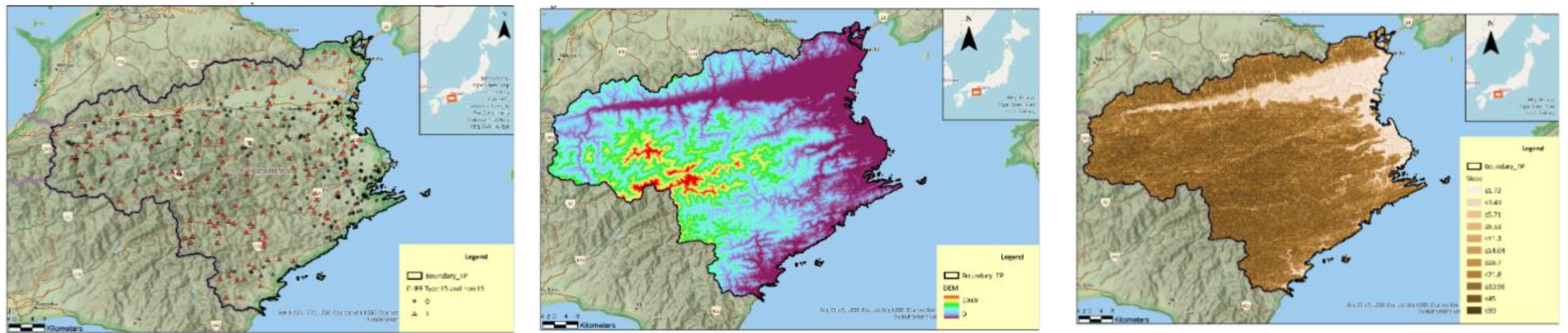
167 Cliff type LS and 167 Non LS points were used to created Cliff type LS occurred, and none occurred point layer. TP elevation ranges from 0-1959m.Graduate color scheme used in Slope map where slope is increasing when brown color become dark.
Figure 8.
Profile curvature/ Plan curvature and Direct duration Radiation of TP shown sequentially.
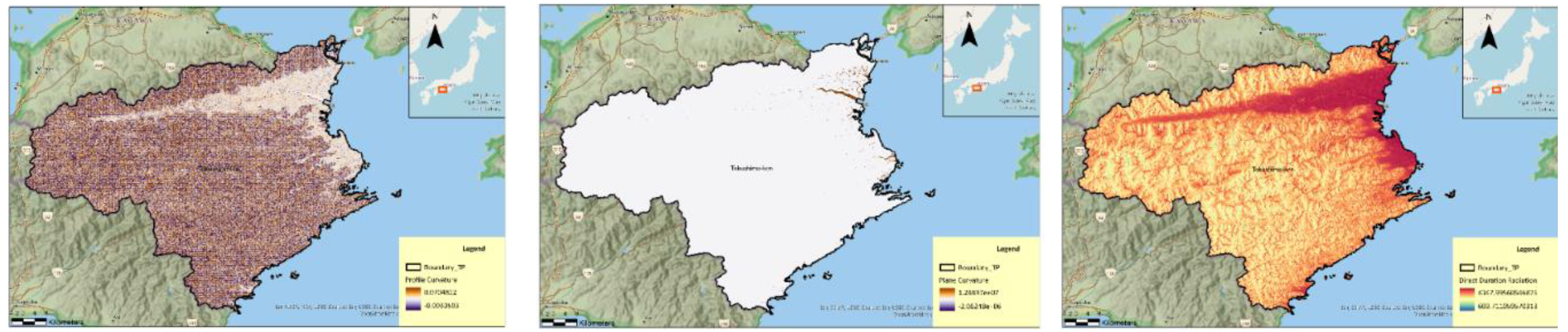
In Profile Curvature Map, Positive values indicate areas of acceleration of surface flow and erosion while negative profile curvature indicates areas of slowing surface flow and deposition. Plan Curvature Map shows a positive value indicates that the surface is laterally convex at that cell. A negative plan indicates that the surface is laterally concave at that cell. A value of zero indicates that the surface is linear. Direct Duration Radiation map represents the duration of direct incoming solar radiation. The output is measured in hours. It indicates how long a location receives direct sunlight over a specified period.
Figure 9.
Direct Radiation/ Flow Direction and Flow Accumulation of TP shown sequentially.
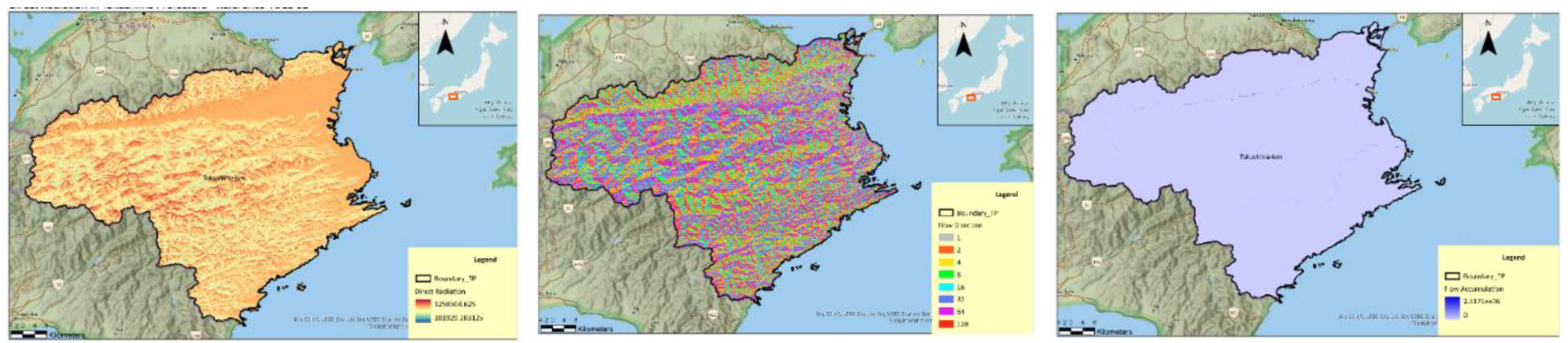
The output of the direct radiation layer represents the direct incoming solar radiation value for each location. The units for this output are kilowatt hours per square meter (kWh/m²). This layer helps in understanding the amount of solar energy received directly from the sun at different locations on the surface. Flow direction from each cell to its downslope neighbor, or neighbors. There are eight valid output directions relating to the eight adjacent cells into which flow could travel (Figure 11). This approach is commonly referred to as an eight-direction (D8). Flow Accumulation represents the accumulation of flow to each cell in the output raster. Higher values indicate areas where more flow accumulates, typically in valleys or stream channels. A color ramp that ranges from low accumulation (light blue) to high accumulation (dark blue).
Figure 10.
Topographical Wetness Index/ Topographical Position Index and Sediment Transportation Index of TP shown sequentially.
Figure 10.
Topographical Wetness Index/ Topographical Position Index and Sediment Transportation Index of TP shown sequentially.
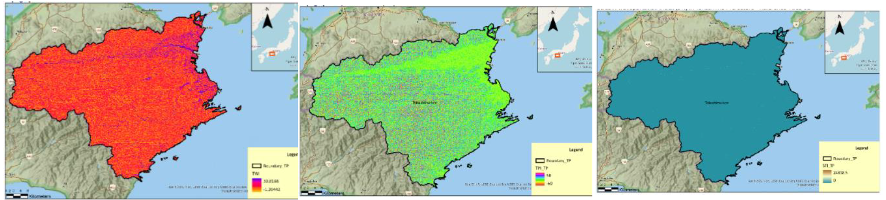
Figure 11.
Direction coding.

TWI is a measure of the spatial distribution of soil moisture. Higher TWI values indicate areas that are likely to be wetter, while lower values indicate drier areas. The distribution of wetness will display using a gradient color ramp. TWI layer ranges from dry (yellow) to wet ( blue). In Topographical Position Index map ppositive TPI Values: Indicate that the cell is higher than its surroundings, typically representing ridges or hilltops. Negative TPI Values: Indicate that the cell is lower than its surroundings, typically representing valleys or depressions. TPI Values Near Zero: Indicate that the cell is at a similar elevation to its surroundings, typically representing flat or gently sloping areas. High STI values indicate areas with high sediment transport potential, likely to be wet. Low STI values indicate areas with low sediment transport potential, likely to be dry in Sediment Transportation Index map.
Figure 12.
Stream Power Index / Topographical Roughness Index and Distance from Streams of TP shown sequentially.
Figure 12.
Stream Power Index / Topographical Roughness Index and Distance from Streams of TP shown sequentially.
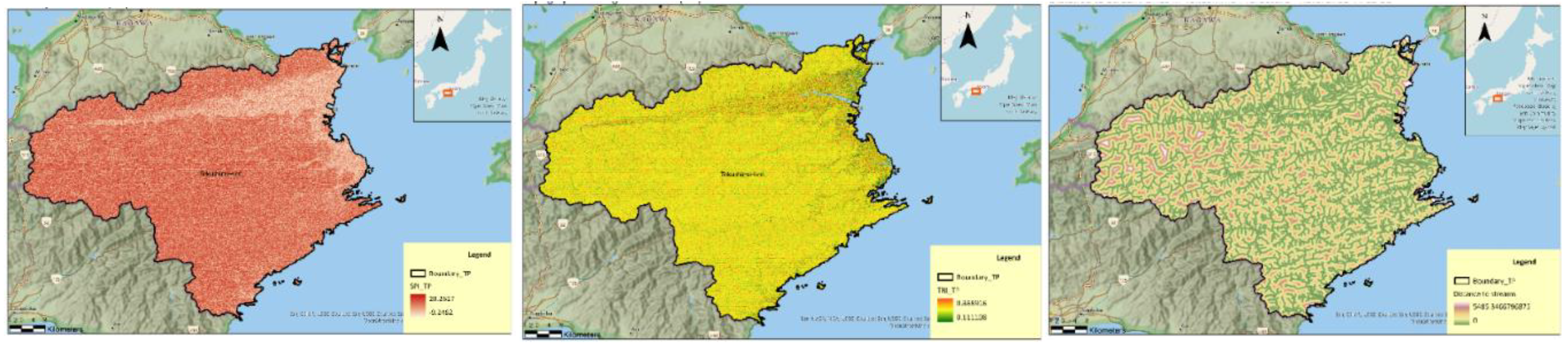
In Stream Power Index map higher SPI values indicate areas with greater potential for erosion, typically found in steep and high-flow areas. positive values suggesting higher erosive potential and negative values indicating sediment accumulation. The distribution of stream power, symbolize the layer using a gradient color ramp. A color ramp that ranges from low power (light brown) to high power (dark brown). High TRI Values: Indicate areas with significant elevation changes between adjacent cells, representing rugged terrain such as steep slopes, cliffs, or mountainous regions. Low TRI Values: Indicate areas with minimal elevation changes between adjacent cells, representing flat or gently rolling terrain in Topographical Roughness Index map.
Figure 13.
Distance from Faults/Distance from Buildings and Distance from Roads of TP shown sequentially.
Figure 13.
Distance from Faults/Distance from Buildings and Distance from Roads of TP shown sequentially.
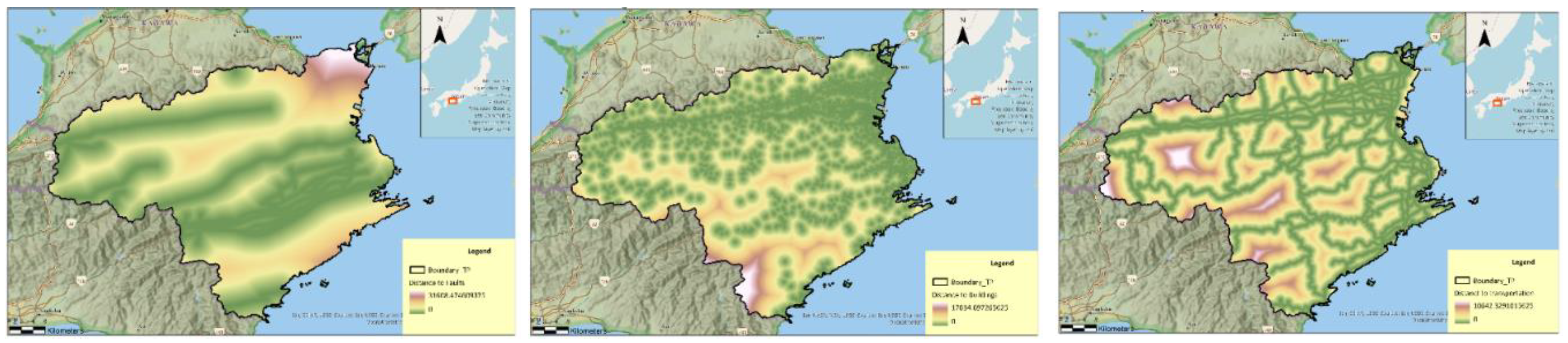
Initially Fault, Building and transportation lines layers were created. Distance layers were created using distance accumulation tool in GIS.In the color scheme green color shows when relevant feature is overlaid on the pixel while white color show when feature is far from the pixel.
Figure 14.
Aspect/ Soil Thickness and NDVI of TP shown sequentially.
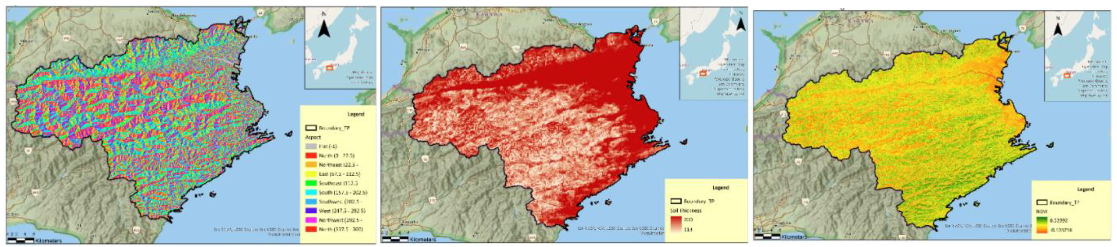
Value Range: NDVI values typically range from -1 to 1. Values close to 1 indicate healthy, dense vegetation. Values close to 0 indicate barren areas of rock, sand, or urban areas. Negative values indicate water, snow, or clouds. color scheme displays colors from green (healthy vegetation) to red (barren areas).
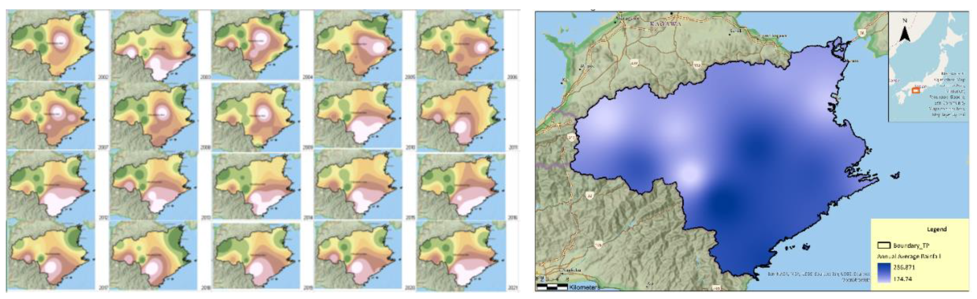
Figure 15.
Year wise Annual Average Rainfall layers and Sum of Annual Average Rainfall for 20 years of TP shown sequentially.
Figure 15.
Year wise Annual Average Rainfall layers and Sum of Annual Average Rainfall for 20 years of TP shown sequentially.
3.1.2. Trained Model Output
Figure 16.
Validation Data Classification Diagnostics and Validation Accuracy Graph of the trained Model sequentially.
Figure 16.
Validation Data Classification Diagnostics and Validation Accuracy Graph of the trained Model sequentially.
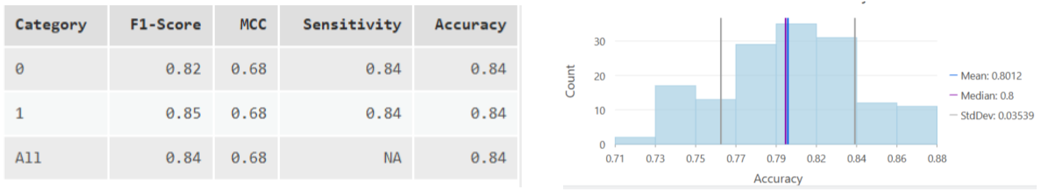
Matthews Correlation Coefficient (MCC = 0.68): MCC is a balanced measure that considers true and false positives and negatives. It ranges from -1 to 1, where 1 indicates perfect prediction, 0 indicates random prediction, and -1 indicates total disagreement between prediction and observation. An MCC of 0.68 suggests that the model has a good level of predictive power, though there is room for improvement. F1 Score (0.84): The F1 Score is the harmonic mean of precision and recall. It ranges from 0 to 1, with higher values indicating better performance. An F1 Score of 0.84 indicates that the model balances precision (correct positive predictions) and recall (ability to find all positives) well, making it reliable for classification tasks.
Sensitivity (0.84): also known as recall or true positive rate, measures the proportion of actual positives correctly identified. A sensitivity of 0.84 means that the model correctly identifies 84% of the positive cases, which is strong performance. Accuracy (0.84): measures the proportion of total predictions (both positive and negative) that are correct. With an accuracy of 0.84, the model correctly predicts 84% of all cases. Mean (0.80) and Median (0.80): These values summarize the central tendency of the model's performance metrics across multiple runs or folds.
A mean and median of 0.80 suggest consistent performance, with no significant outliers skewing the results. Standard Deviation (0.03):the variability or spread of the performance metrics. A standard deviation of 0.03 indicates that the model's performance is stable and does not vary much across different runs or folds.As a summary Random Forest model demonstrates strong and consistent performance with good sensitivity, F1 Score, and accuracy. The MCC value further confirms that the model is making balanced predictions.
Figure 17.
Prediction Performance Graph/ Confusion Matrix and Validation Performance Graph of the trained Model sequentially.
Figure 17.
Prediction Performance Graph/ Confusion Matrix and Validation Performance Graph of the trained Model sequentially.
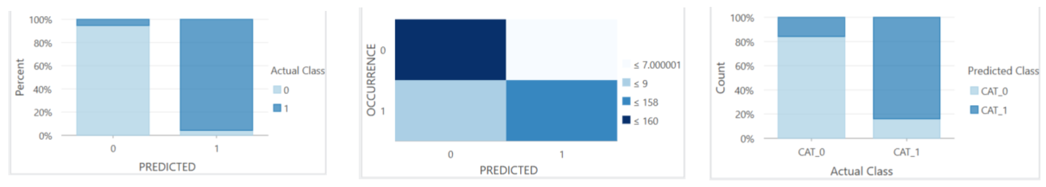
In the Prediction Performance Graph, the model achieves 95% prediction performance for both landslide and non-landslide classes, it indicates that the model is highly effective at distinguishing between the two categories and is not biased toward one class. Sensitivity (Recall for Landslide): Measures how well the model identifies actual landslides. Specificity (Recall for Non-Landslide): Measures how well the model identifies actual non-landslides. If both sensitivity and specificity are close to 95%, it confirms balanced performance. In summary, a 95% prediction performance for both landslide and non-landslide classes indicates a highly effective and balanced model.
This confusion Matrix represents 7 out of 334, non-landslide predicted as landslide while 9 in wise versa.7 False positives cases. These are instances where the model incorrectly predicted non-landslide areas as landslide. This suggests the model is slightly over-predicting landslides, which could be useful in cautious scenarios but might lead to unnecessary mitigation efforts in areas that are not at risk. While 9 False negatives cases are instances where the model failed to predict actual landslide areas (classified them as non-landslide). This is more critical because missing actual landslide areas could result in unpreparedness and potential risks to life and property.
The validation performance graph showing 85% accuracy for both landslide and non-landslide classes indicates that the model is performing well and is balanced in its predictions. This is a good indication of the model's overall reliability. Since the accuracy is the same for both classes, the model is not biased toward predicting one class over the other. This balance is crucial in cases where both types of predictions are equally important.
Unlike previous models that target landslides of all types, the current study focuses specifically on cliff-type landslides. This narrower focus introduces modeling constraints, including reduced data availability. Nonetheless, the model’s performance ( Accuracy = 0.84, MCC = 0.68) compares favorably with broader studies, suggesting strong generalization even within this specialized domain. This specialization enhances the model's relevance to apply appropriate countermeasures. In conventional landslide susceptibility modeling, the focus is often on detecting the likelihood of any type of landslide occurrence. However, such general models do not distinguish between different landslide mechanisms—each of which requires distinct countermeasures. For example, mitigation strategies for debris flows differ significantly from those needed for cliff-type or rockfall events. Predicting cliff-type susceptibility with greater spatial precision allows engineers and planners to design and apply appropriate site-specific countermeasures, thereby improving hazard mitigation effectiveness and resource efficiency.
Moreover, if the landslide type is unknown, applying countermeasures becomes a process of guesswork, which may lead to ineffective or even hazardous outcomes. Thus, this research aim was to bridge the gap between landslide susceptibility mapping and practical engineering application.
Figure 18.
Distribution of Variable Importance of the trained Model.
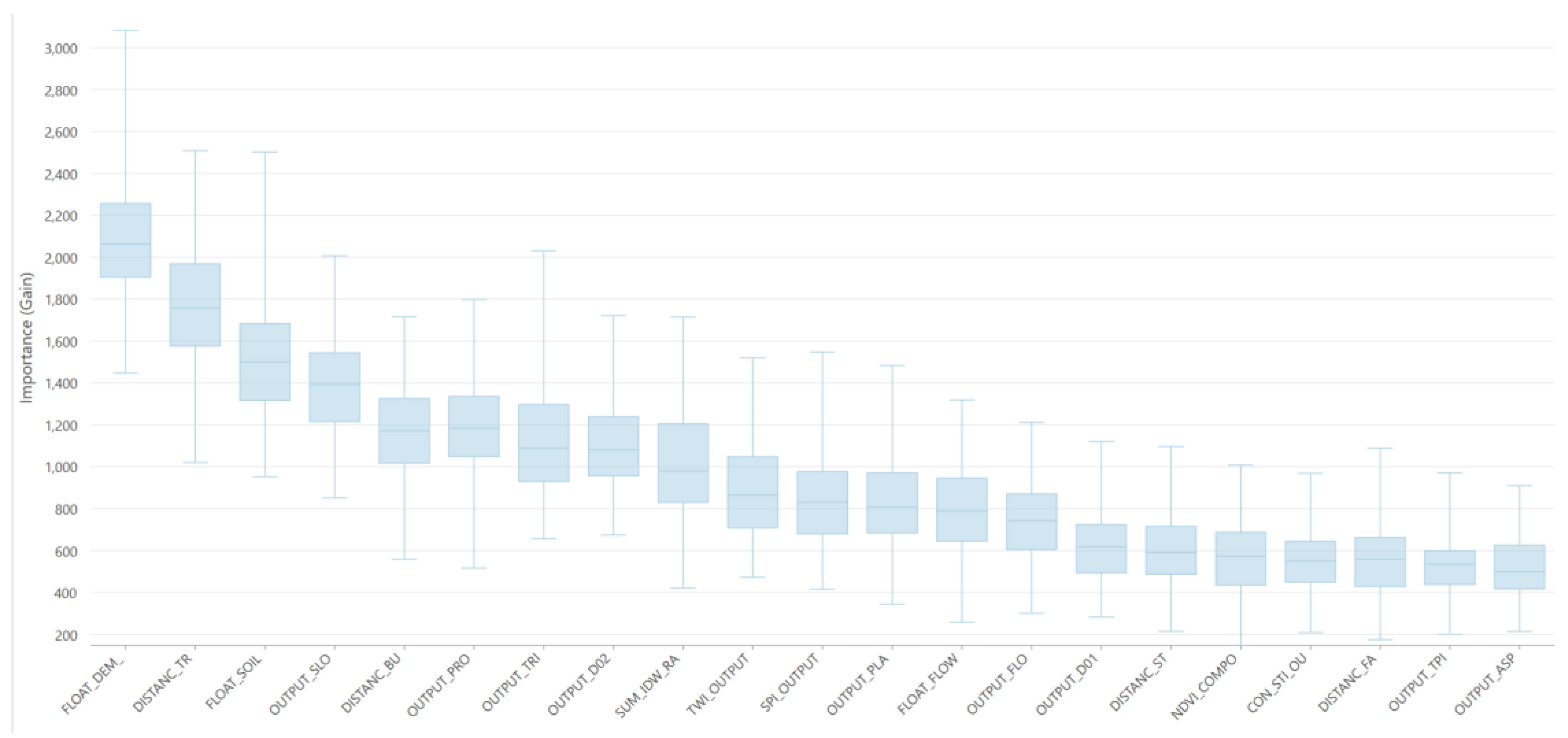
Distribution of variable importance provides insights into how different input features (variables) contribute to the model's predictions. DEM, Distance from Transportation lines, Soil thickness, Slope and Distance from Buildings are the first five LCF while Aspect , TPI, Distance from faults, STI and NDVI are the least five LCF in the current Model [1,10,14,15,17,18,20,24,25,27,28,30,31,34,35,36,39,42,43,44,47,51]
3.2. Predict to Tokushima Prefecture Subarea
3.2.1. Predicted Raster Layer
Forest-based and Boosted Classification and Regression tool in GIS Pro was used by changing prediction type from train only to predict to raster. Raster output location was saved under geodatabase. Subarea of TP was selected where high Cliff LS occurred in the past for the prediction as shown below Figure 19. All 21 layers were created using clip raster tool in GIS. 21 explanatory variable layers were created (Figure 20) for TP subarea and used match explanatory raster in the trained Model in FRBC tool.
Figure 19.
Selected subarea of TP for the prediction.
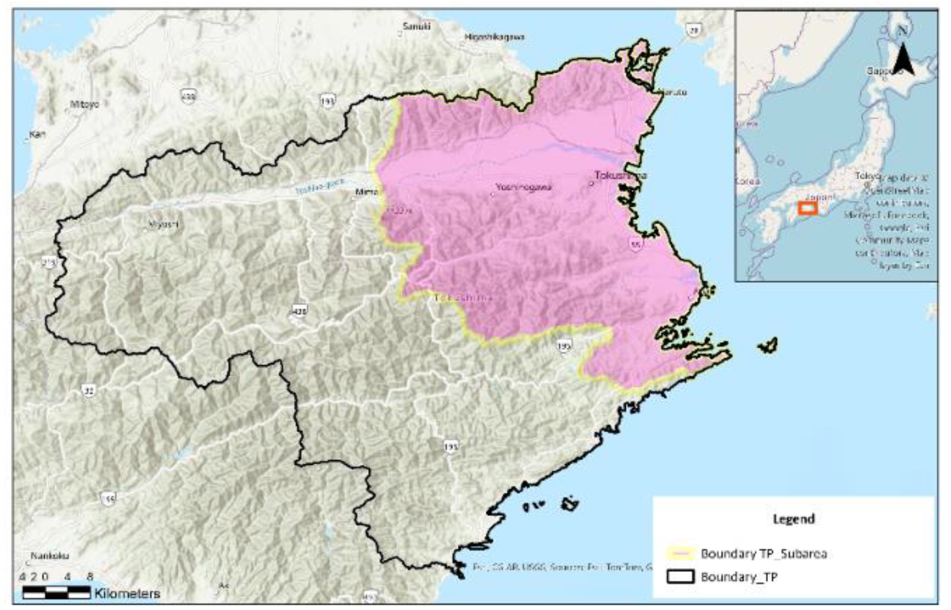
Figure 20.
Aspect, DEM, Profile Curvature, Plan Curvature, Direct Duration Radiation, Direct Radiation, Flow Direction, Flow Accumulation, TWI, TPI, STI, SPI, TRI, Distance from Streams, Distance from Faults, Distance from Buildings, Distance from Roads, Soil thickness, NDVI, Annual Average and Slope of TP subarea sequentially.
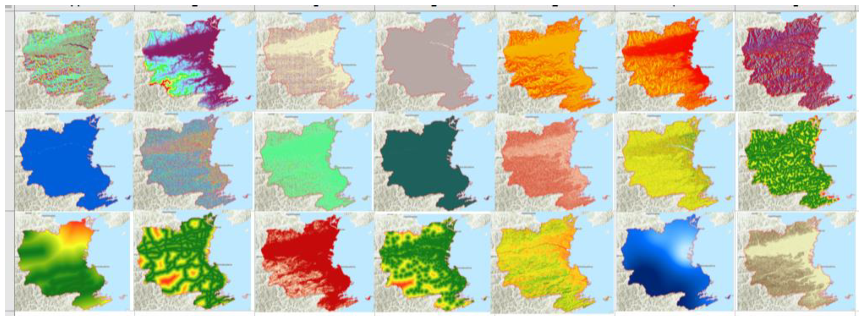
Figure 21.
Predicted Map for Cliff type LS in subarea 01 of TP by the Model.
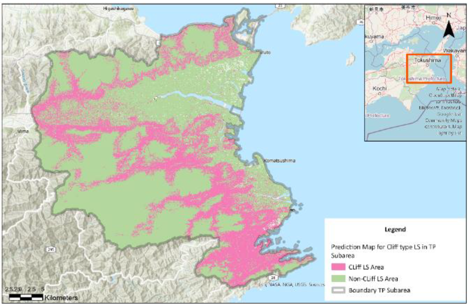
Pink color represent the predicted cliff type LS area while green color represents predicted non cliff type LS area by the trained model for TP subarea.
3.2.2. Validate the Predicted Layer Referring TP Inventory; Only 70% Points Used to Train the Model
Figure 22.
Validation of predicted Cliff type LS area referring TP inventory in subarea.
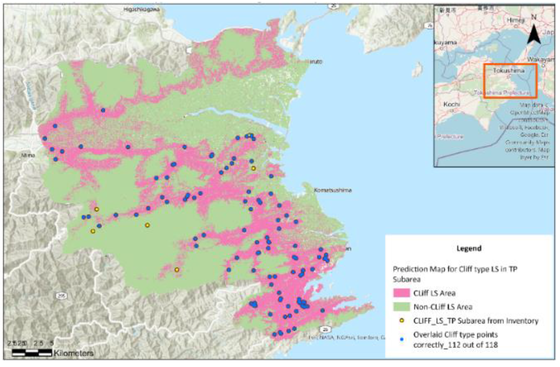
112 points out of 118 cliff type LS points were overlaid on predicted cliff type LS area in TP subarea which shows 95% accuracy by tallying exactly with Prediction Performance Graph output of the model trained. This shows that Model is performing well in a scenario like Landslide occurrence.
3.3. Predict to Kegalle District
3.3.1. Predicted Raster Layer
Forest-based and Boosted Classification and Regression tool in GIS Pro was used by changing prediction type from train only to predict to raster. Raster output location was saved under geodatabase. All 21 layers were created using tools in GIS using same steps to create TP layers as explained above. Created 21 explanatory variable layers (Figure 23) were loaded under match explanatory raster in the trained Model in FRBC tool.
Figure 23.
Aspect, DEM, Slope. Profile Curvature, Plan Curvature, Direct Duration Radiation, Direct Radiation, Flow Direction, Flow Accumulation, TWI, TPI, STI, SPI, TRI, Distance from Streams, Distance from Faults, Distance from Buildings, Distance from Roads, Soil thickness, NDVI and Annual Average of KD sequentially.
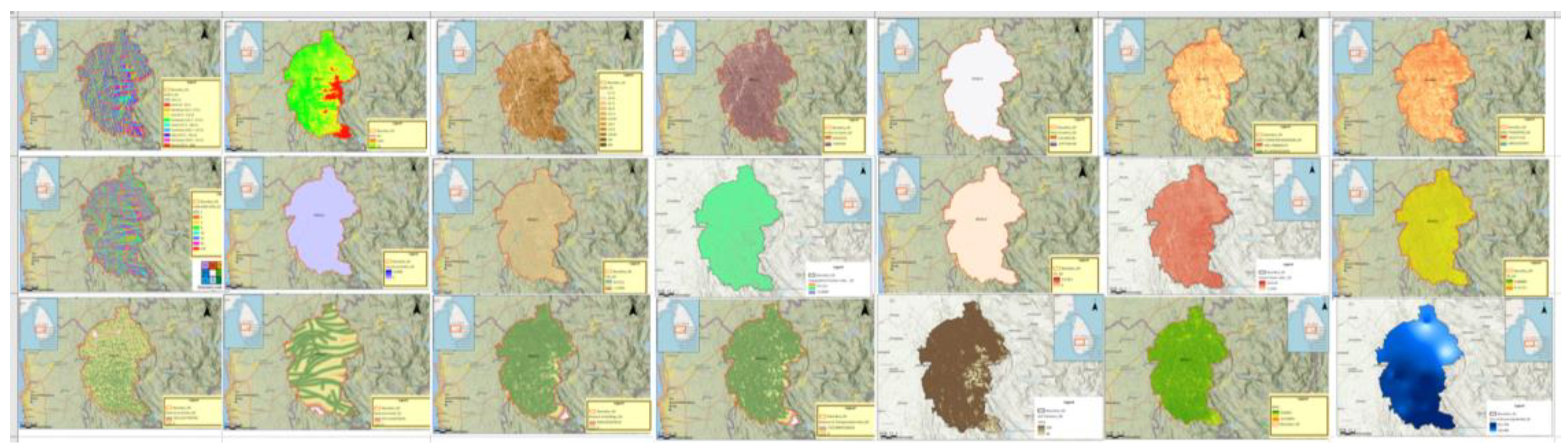
Figure 24.
Predicted Map for Cliff type LS in KD by the Model.
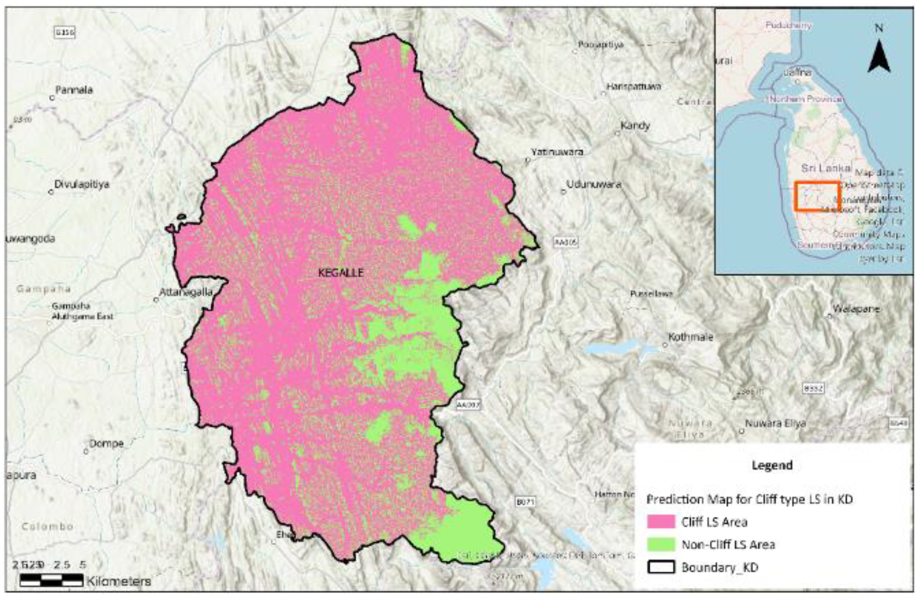
Pink color represent the predicted cliff type LS area while green color represents predicted non cliff type LS area by the trained model for KD.
3.3.2. Validate the Predicted Layer Referring KD Recently Modified Inventory
Figure 25.
LS type classified recently modified inventory KD map and Validation of predicted Cliff type LS area referring recently modified KD Inventory map sequentially.
Figure 25.
LS type classified recently modified inventory KD map and Validation of predicted Cliff type LS area referring recently modified KD Inventory map sequentially.
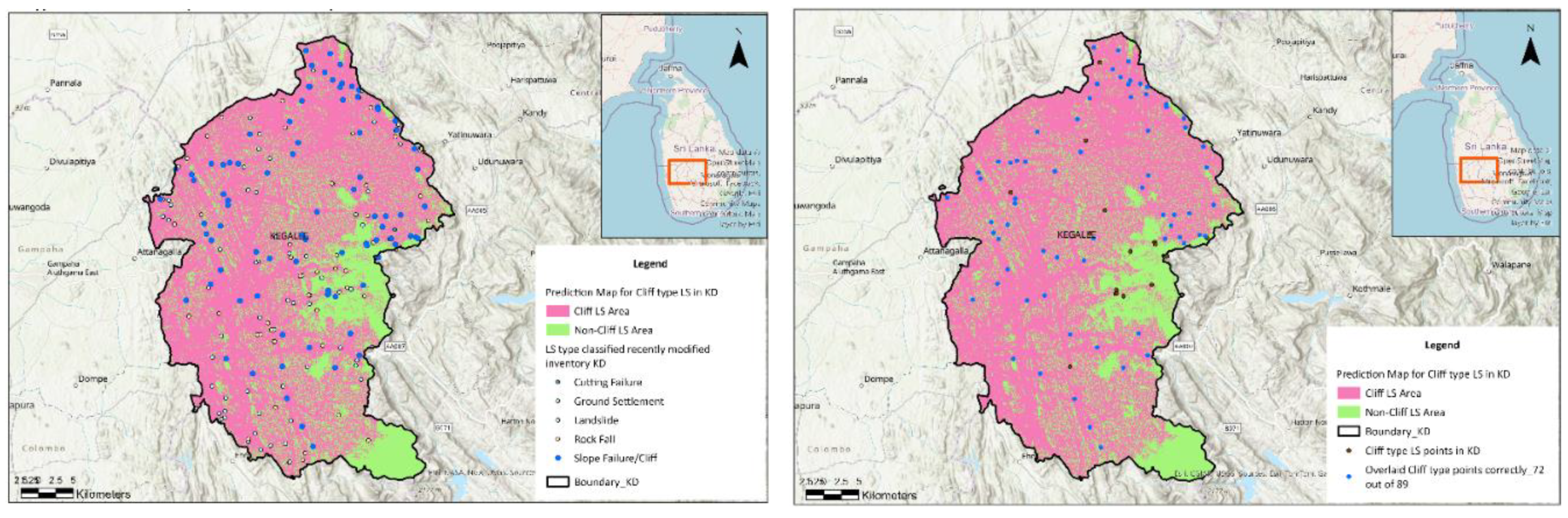
Recently modified inventory in KD has 89 cliff type LS points. 72 out of 89 cliff type LS points were overlaid on predicted cliff type LS area in K by showing 80.1% accuracy. This shows that Model is performing well in a scenario like Landslide occurrence. The English word "landslide" refers to three major phenomena in Japan.In Japan, landslides in English are broadly classified into debris flow, landslides, and slope failure (cliff) [40]. In Sri Lanka four types of landslides have been recognized and classified from past landslide inventory, including slides, slope failures, debris flows and rockfalls [41]. Both countries definition for slope failure (cliff) and landslide (slide in Sri Lanka) is similar.
3.3.3. Predict Cliff Type LS Before Modifying the Inventory Incidents in Kegalle District
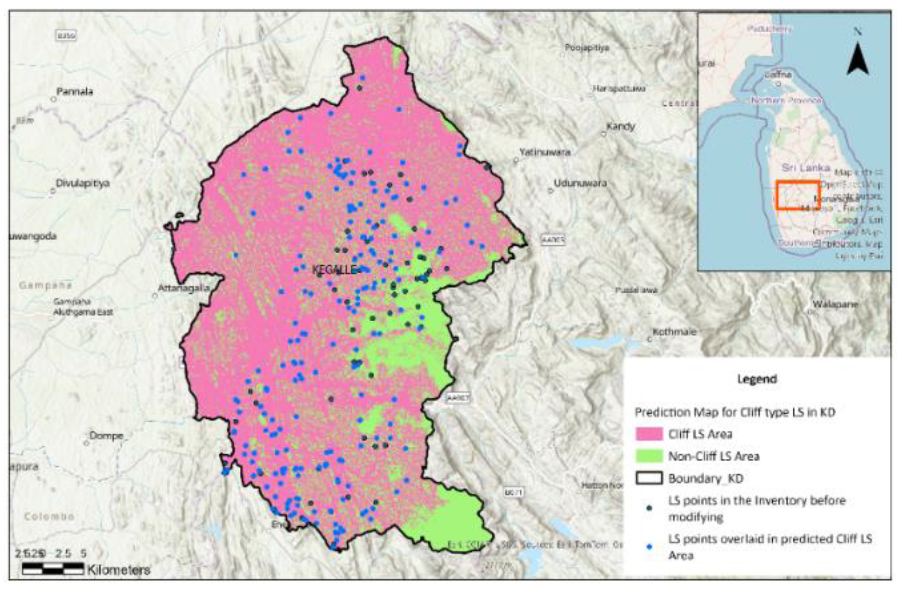
Figure 26.
LS points overlaid on the predicted cliff type LS area referring KD inventory before modifying recently.
Figure 26.
LS points overlaid on the predicted cliff type LS area referring KD inventory before modifying recently.
4. Conclusion
Elevation, rainfall, aspect, slope, profile curvature, TWI, STI, SPI, NDVI, plane curvature, TPI, TRI, direct radiation, duration of direct radiation, flow accumulation, flow direction, soil thickness and distance from faults, from roads, from water bodies, from structures ;21 Landslide conditioning factors were used to train the Model using Forest-based and Boosted Classification and Regression tools within ArcGIS Pro software. Soil type, Geology and Land use LCF were removed while training the model due to the least importance to the Cliff type LS occurrence. Tokushima Prefecture was used to train the Model.TP has similar ranges of elevation and annual average rainfall to Kegalle District. Also, earthquake induced Cliff LS were not found in TP.
The model shows a mean of 0.80, a median of 0.80, a standard deviation of 0.03, an accuracy of 0.84, a sensitivity of 0.84, MCC of 0.68, and F1 score of 0.84 by indicating the Model is overall the model can be considered robust, accurate, and generalizable, making it suitable for operational use in Cliff type landslide prediction and related decision-making processes. Prediction performance of 95% is excellent and suggests that the model is highly effective at making accurate predictions. A validation performance of 85% indicates that the model generalizes reasonably well to data it hasn't seen during training.
Distribution of variable importance provides that DEM, Distance from Transportation lines, Soil thickness, Slope and Distance from Buildings are the first five triggering Cliff LCF while Aspect, TPI, Distance from faults, STI and NDVI are the least five LCF.
The Model was used to predict subarea of TP itself, because only 70% of data used to train the Model. Prediction parameters shows that the model performs well in prediction by overlaying 95% points match accurately with TP inventory by tallying the the model output prediction performance graph. The model was used to predict to Kegalle district. Predicted layer was overlaid with recently modified inventory points and shows 80.1%points match accurately. Prediction was made for the inventory before modifying in KD.
This model aid in identifying cliff-type landslides from inventories where landslide type is not listed to apply appropriate countermeasures to prevent future occurrences. Moreover, predicting cliff-type susceptibility with greater spatial precision allows engineers and planners to design and apply appropriate site-specific countermeasures, thereby improving hazard mitigation effectiveness and resource efficiency. If the landslide type is unknown, applying countermeasures becomes a process of guesswork, which may lead to ineffective or even hazardous outcomes. Thus, this research aim was to bridge the gap between landslide susceptibility mapping and practical engineering application.
5. Limitations
While the model shows robust performance metrics, several limitations should be acknowledged. First, the quality and completeness of the landslide inventory and Earthquake inventory used for training may introduce bias, as undetected or misclassified landslide events could affect the model’s learning process. Additionally, the environmental variables used were limited to available spatial layers, potentially omitting relevant but unmeasured factors such as Soil Water Index and Ground Water level. Lastly, although Cliff LS point layer and 21 LCF considered, only Earthquake point layer was considered with a buffer drawn to outside from the TP area.
6. Recommendations
To improve the comprehensiveness and practical value of landslide susceptibility modeling, it is recommended to integrate temporal variables such as rainfall intensity, earthquake occurrences, and historical landslide timing into future models. Incorporating these time-dependent factors would enable the prediction of not only spatial risk but also the likely timing of landslide events. Additionally, future studies should aim to develop models specifically tailored for earthquake-affected areas, as seismic activity plays a critical role in triggering landslides, particularly in steep and unstable terrain. Furthermore, extending the modeling approach to include various types of landslides—such as debris flows.
Author Contributions
Not applicable.
Funding
Not applicable.
Institutional Review Board Statement
Not applicable.
Informed Consent Statement
Not applicable.
Data Availability Statement
The original contributions presented in this study are included in the article. Further inquiries can be directed to the corresponding author.
Acknowledgments
The authors would like to thank all the people and organizations who contributed to make this research successfully, especially the Professors at Saitama University, Professor Maros Finka from Slovakia, Dr. Asiri and Mr. Sivanantharajah from Sri Lanka, Dr. Tina and Dr, Ziad from UK and Mr. Jack Horton from USA who gave valuable insight.
Conflicts of Interest
The authors declare no conflict of interest.
Abbreviations
The following abbreviations are used in this manuscript:
| FRCB | Forest-based and Boosted Classification and Regression |
| KD | Kegalle District |
| LS | Landslide |
| LCF | Landslide Conditioning Factors |
| MCC | Matthew’s correlation coefficient |
| NDVI | Normalized difference vegetation index |
| NBRO | National Building Research Organization |
| RA | Reference Area |
| STI | Sediment transportation index |
| SPI | Stream power index |
| SA | Study Area |
| TP | Tokushima Prefecture |
| TPI | Topographical position index |
| TRI | Topographical roughness index |
| TWI | Topographical wetness index |
| WP | Wakayama Prefecture |
References
- Achour, Y.; Saidani, Z.; Touati, R.; Pham, Q.B.; Pal, S.C.; Mustafa, F.; Balik Sanli, F. Assessing landslide susceptibility using a machine learning-based approach to achieving land degradation neutrality. Environmental Earth Sciences 2021, 80, 17. [Google Scholar] [CrossRef]
- Ali, S.A.; Parvin, F.; Vojteková, J.; Costache, R.; Linh, N.T.T.; Pham, Q.B.; Vojtek, M.; Gigović, L.; Ahmad, A.; Ghorbani, M.A. GIS-based landslide susceptibility modeling: A comparison between fuzzy multi-criteria and machine learning algorithms. Geoscience Frontiers 2021, 12, 857–876. [Google Scholar] [CrossRef]
- AMeDAS. Available online: https://www.jma.go.jp/jma/en/Activities/amedas/amedas.html (accessed on 10 July 2025).
- Bandara, R.M.S.; Jayasingha, P. Landslide disaster risk reduction strategies and present achievements in Sri Lanka. Geosciences Research 2018, 3, 3. [Google Scholar] [CrossRef]
- Bennett, G.L.; Miller, S.R.; Roering, J.J.; Schmidt, D.A. Landslides, threshold slopes, and the survival of relict terrain in the wake of the Mendocino Triple Junction. Geology 2016, 44, 363–366. [Google Scholar] [CrossRef]
- Brenning, A. Spatial prediction models for landslide hazards: review, comparison and evaluation. Nat. Hazards Earth Syst. Sci. 2005, 5, 853–862. [Google Scholar] [CrossRef]
- Chen, W.; Xie, X.; Wang, J.; Pradhan, B.; Hong, H.; Bui, D.T.; Duan, Z.; Ma, J. A comparative study of logistic model tree, random forest, and classification and regression tree models for spatial prediction of landslide susceptibility. Catena 2017, 151, 147–160. [Google Scholar] [CrossRef]
- Dang, V.H.; Hoang, N.D.; Nguyen, L.M.D.; Bui, D.T.; Samui, P. A novel GIS-based random forest machine algorithm for the spatial prediction of shallow landslide susceptibility. Forests 2020, 11, 1. [Google Scholar] [CrossRef]
- Democratic Socialist Republic of Sri Lanka. Project for Capacity Strengthening on Development of Non-Structural Measures for Landslide Risk Reduction in Sri Lanka. 2022.
- Dhungana, G.; Ghimire, R.; Poudel, R.; Kumal, S. Landslide susceptibility and risk analysis in Benighat Rural Municipality, Dhading, Nepal. Nat. Hazards Res. 2023, 3, 170–185. [Google Scholar] [CrossRef]
- Download site for digital land information. Available online: https://nlftp.mlit.go.jp/ksj/index.html (accessed on 10 July 2025).
- Esri Academy. Available online: https://www.esri.com/training/ (accessed on 10 July 2025).
- Forest-based and Boosted Classification and Regression (Spatial statistics). Available online: https://pro.arcgis.com/en/pro-app/latest/tool-reference/spatial-statistics/forestbasedclassificationregression.htm (accessed on 10 July 2025).
- Goetz, J.N.; Brenning, A.; Petschko, H.; Leopold, P. Evaluating machine learning and statistical prediction techniques for landslide susceptibility modeling. Comput. Geosci. 2015, 81, 1–11. [Google Scholar] [CrossRef]
- Guo, Z.; Ferrer, J.V.; Hürlimann, M.; Medina, V.; Puig-Polo, C.; Yin, K.; Huang, D. Shallow landslide susceptibility assessment under future climate and land cover changes: A case study from southwest China. Geoscience Frontiers 2023, 14, 4. [Google Scholar] [CrossRef]
- Haque, U.; Blum, P.; da Silva, P.F.; Andersen, P.; Pilz, J.; Chalov, S.R.; Malet, J.P.; Auflič, M.J.; Andres, N.; Poyiadji, E.; et al. Fatal landslides in Europe. Landslides 2016, 13, 1545–1554. [Google Scholar] [CrossRef]
- He, Q.; Shahabi, H.; Shirzadi, A.; Li, S.; Chen, W.; Wang, N.; Chai, H.; Bian, H.; Ma, J.; Chen, Y.; et al. Landslide spatial modelling using novel bivariate statistical based Naïve Bayes, RBF Classifier, and RBF Network machine learning algorithms. Sci. Total Environ. 2019, 663, 1–15. [Google Scholar] [CrossRef]
- He, Q.; Xu, Z.; Li, S.; Li, R.; Zhang, S.; Wang, N.; Pham, B.T.; Chen, W. Novel entropy and rotation forest-based credal decision tree classifier for landslide susceptibility modeling. Entropy 2019, 21, 2. [Google Scholar] [CrossRef] [PubMed]
- Hemasinghe, H.; Rangali, R.S.S.; Deshapriya, N.L.; Samarakoon, L. Landslide susceptibility mapping using logistic regression model (a case study in Badulla District, Sri Lanka). Procedia Eng. 2018, 212, 1046–1053. [Google Scholar] [CrossRef]
- Hu, H.; Wang, C.; Liang, Z.; Gao, R.; Li, B. Exploring complementary models consisting of machine learning algorithms for landslide susceptibility mapping. ISPRS Int. J. Geo-Inf. 2021, 10, 639. [Google Scholar] [CrossRef]
- Huang, F.; Cao, Z.; Guo, J.; Jiang, S.H.; Li, S.; Guo, Z. Comparisons of heuristic, general statistical and machine learning models for landslide susceptibility prediction and mapping. Catena 2020, 191, 104580. [Google Scholar] [CrossRef]
- ISRIC World Soil Information. Available online: https://data.isric.org/geonetwork/srv/eng/catalog.search#/metadata/f36117ea-9be5-4afd-bb7d-7a3e77bf392a (accessed on 10 July 2025).
- ISRIC World Soil Information. Available online: https://www.isric.org/explore/soilgrids/faq-soilgrids#What_happened_to_the_maps_of_soil_types (accessed on 10 July 2025).
- Kaihara, S.; Tadakuma, N.; Saito, H.; Nakaya, H. Influence of below-threshold rainfall on landslide occurrence based on Japanese cases. Natural Hazards 2023, 115, 2307–2332. [Google Scholar] [CrossRef]
- Kalantar, B.; Ueda, N.; Saeidi, V.; Ahmadi, K.; Halin, A.A.; Shabani, F. Landslide susceptibility mapping: Machine and ensemble learning based on remote sensing big data. Remote Sens. 2020, 12, 11. [Google Scholar] [CrossRef]
- Keefer, D.K. Landslides Caused by Earthquakes. Geol. Soc. Am. Bull. 1984, 95, 406–421. [Google Scholar] [CrossRef]
- Kohno, M.; Higuchi, Y. Landslide Susceptibility Assessment in the Japanese Archipelago Based on a Landslide Distribution Map. ISPRS Int. J. Geo-Inf. 2023, 12, 2. [Google Scholar] [CrossRef]
- Kumar, C.; Walton, G.; Santi, P.; Luza, C. An Ensemble Approach of Feature Selection and Machine Learning Models for Regional Landslide Susceptibility Mapping in the Arid Mountainous Terrain of Southern Peru. Remote Sens. 2023, 15, 1376. [Google Scholar] [CrossRef]
- Kumarihamy, R.M.K.; Nianthi, K.W.G.R.; Shaw, R. Land Cover Changes and Landslide Risk in Sri Lanka 2022, pp. 413–433. [CrossRef]
- Liang, Z.; Wang, C.; Khan, K.U.J. Application and comparison of different ensemble learning machines combining with a novel sampling strategy for shallow landslide susceptibility mapping. Stoch. Environ. Res. Risk Assess. 2021, 35, 1243–1256. [Google Scholar] [CrossRef]
- Miao, F.; Zhao, F.; Wu, Y.; Li, L.; Török, Á. Landslide susceptibility mapping in Three Gorges Reservoir area based on GIS and boosting decision tree model. Stoch. Environ. Res. Risk Assess. 2023. [Google Scholar] [CrossRef]
- Modugno, S.; Johnson, S.C.M.; Borrelli, P.; Alam, E.; Bezak, N.; Balzter, H. Analysis of human exposure to landslides with a GIS multiscale approach. Nat. Hazards 2022, 112, 387–412. [Google Scholar] [CrossRef]
- Moresi, F.V.; Maesano, M.; Collalti, A.; Sidle, R.C.; Matteucci, G.; Mugnozza, G.S. Mapping landslide prediction through a GIS-based model: A case study in a catchment in southern Italy. Geosciences 2020, 10, 80309. [Google Scholar] [CrossRef]
- Mosaffaie, J.; Salehpour Jam, A.; Sarfaraz, F. Landslide risk assessment based on susceptibility and vulnerability. Environ. Dev. Sustain. 2023. [CrossRef]
- Nachappa, T.G.; Ghorbanzadeh, O.; Gholamnia, K.; Blaschke, T. Multi-hazard exposure mapping using machine learning for the state of Salzburg, Austria. Remote Sens. 2020, 12, 17. [Google Scholar] [CrossRef]
- Palliyaguru, S.T.; Liyanage, L.C.; Weerakoon, O.S.; Wimalaratne, G.D.S.P. Random forest as a novel machine learning approach to predict landslide susceptibility in Kalutara District, Sri Lanka. In Proceedings of the 20th Int. Conf. on Advances in ICT for Emerging Regions (ICTer); 2020; pp. 262–267. [Google Scholar] [CrossRef]
- Papadopoulos, G.A. , & Plessa, A. Magnitude-distance relations for earthquake-induced landslides in Greece. In Engineering Geology (Vol. 58) 2000. www.elsevier.nl/locate/enggeo.
- Pennington, C.; Dijkstra, T.; Lark, M.; Dashwood, C.; Harrison, A.; Freeborough, K. Antecedent precipitation as a potential proxy for landslide incidence in South West UK. In Proceedings of World Landslide Forum, 2014., Vol. 3.
- Pham, Q.B.; Achour, Y.; Ali, S.A.; Parvin, F.; Vojtek, M.; Vojteková, J.; Al-Ansari, N.; Achu, A.L.; Costache, R.; Khedher, K.M.; Anh, D.T. A comparison among fuzzy multi-criteria decision making, bivariate, multivariate and machine learning models in landslide susceptibility mapping. Geomatics, Nat. Hazards Risk 2021, 12, 1741–1777. [Google Scholar] [CrossRef]
- Project for Capacity Strengthening on Development of Non-Structural Measures for Landslide Risk Reduction in Sri Lanka: National Building Research Organization. Final Report. 2022.
- Protection of Lives from Sediment Disasters: A SABO Supplementary Reader. 2016. Available online: http://www.sabopc.or.jp (accessed on 10 July 2025).
- Qin, Y.; Yang, G.; Lu, K.; Sun, Q.; Xie, J.; Wu, Y. Performance evaluation of five GIS-based models for landslide susceptibility prediction and mapping: A case study of Kaiyang County, China. Sustainability 2021, 13, 11441. [Google Scholar] [CrossRef]
- Saha, S.; Roy, J.; Hembram, T.K.; Pradhan, B.; Dikshit, A.; Maulud, K.N.A.; Alamri, A.M. Comparison between deep learning and tree-based machine learning approaches for landslide susceptibility mapping. Water 2021, 13, 2664. [Google Scholar] [CrossRef]
- Shah, N.A.; Shafique, M.; Ishfaq, M.; Faisal, K.; van der Meijde, M. Integrated approach for landslide risk assessment using geoinformation tools and field data in Hindukush Mountain Ranges, Northern Pakistan. Sustainability 2023, 15, 3102. [Google Scholar] [CrossRef]
- Shinohara, Y.; Watanabe, Y. Differences in factors determining landslide hazards among three types of landslides in Japan. Nat. Hazards 2023, 118, 1689–1705. [Google Scholar] [CrossRef]
- Sri Lankans shouldn’t repeat the same mistake - JICA. Available online: https://www.dailymirror.lk/opinion/sri-lankans-shouldn-t-repeat-the-same-mistake-jica/172-92179 (accessed on 10 July 2025).
- Stanley, T.A.; Kirschbaum, D.B.; Benz, G.; Emberson, R.A.; Amatya, P.M.; Medwedeff, W.; Clark, M.K. Data-driven landslide nowcasting at the global scale. Front. Earth Sci. 2021, 9, 640043. [Google Scholar] [CrossRef]
- USGS EarthExplorer. Available online: https://earthexplorer.usgs.gov/ (accessed on 10 July 2025).
- USGS Earthquake Hazards Program. Available online: https://earthquake.usgs.gov/earthquakes/search/ (accessed on 10 July 2025).
- Vakhshoori, V.; Pourghasemi, H.R.; Zare, M.; Blaschke, T. Landslide susceptibility mapping using GIS-based data mining algorithms. Water 2021, 11, 2292. [Google Scholar] [CrossRef]
- Zhang, W.; He, Y.; Wang, L.; Liu, S.; Meng, X. Landslide susceptibility mapping using random forest and extreme gradient boosting: A case study of Fengjie, Chongqing. Geol. J. 2023. https://doi.org/10.1002/gj.4683.Achour, Y., Saidani, Z., Touati, R., Pham, Q. B., Pal, S. C., Mustafa, F., & Balik Sanli, F. Assessing landslide susceptibility using a machine learning-based approach to achieving land degradation neutrality. Environmental Earth Sciences 2021, 80. [Google Scholar] [CrossRef]
Figure 1.
Kegalle District (KD) - Study Area (SA).
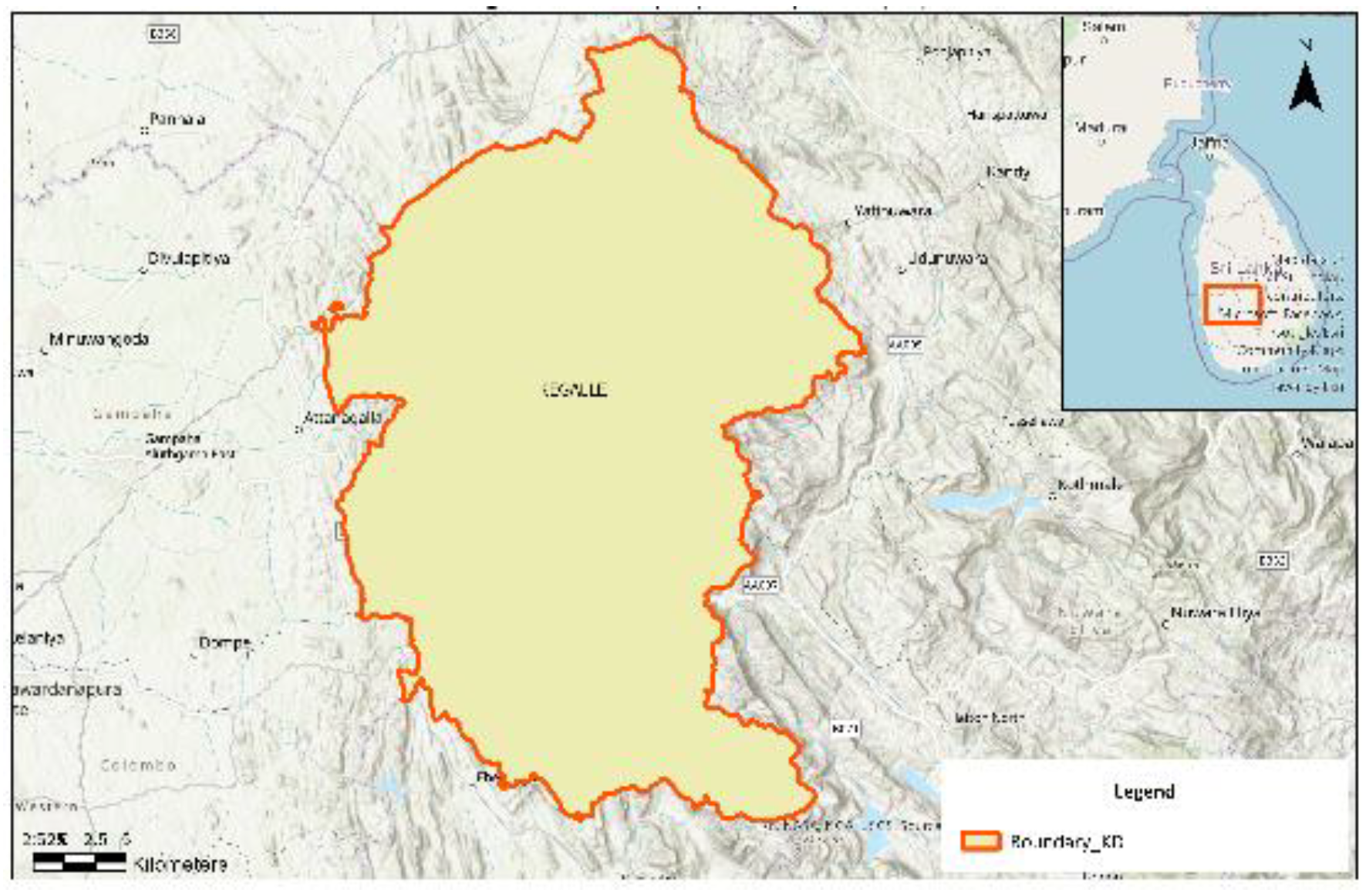
Figure 2.
(a) Number of landslide incidents by district: 1974–2020 [29]; (b) Number of fatalities by district: 1974–2020[29].
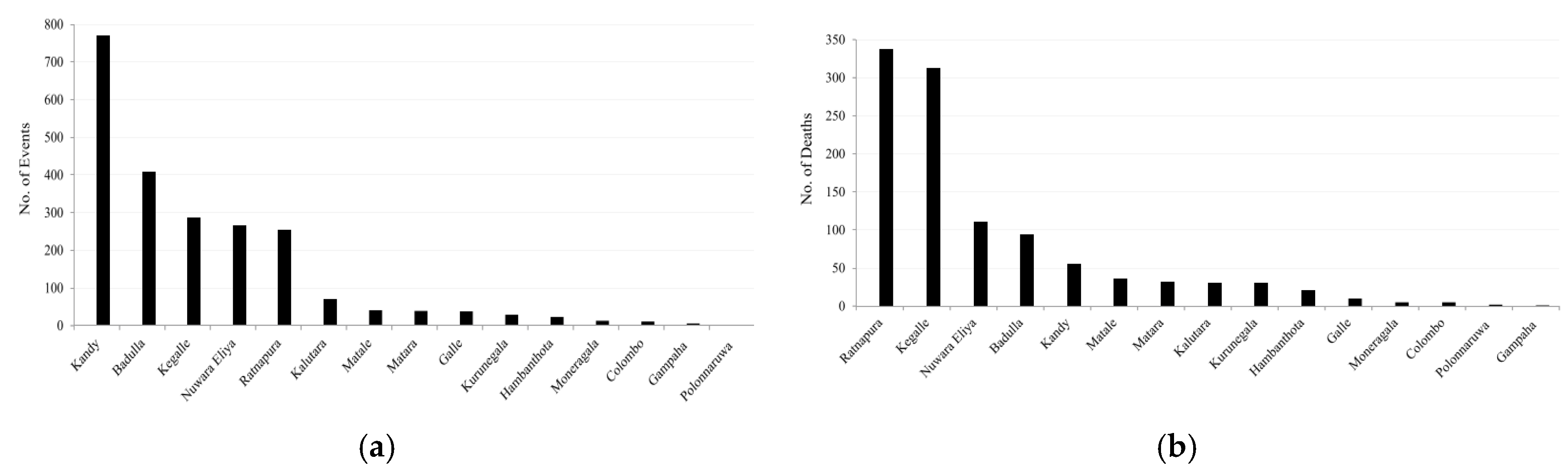
Figure 3.
LCF considered vs conclusions made by past authors. [1,10,14,15,17,18,20,24,25,27,28,30,31,34,35,36,39,42,43,44,47,51].
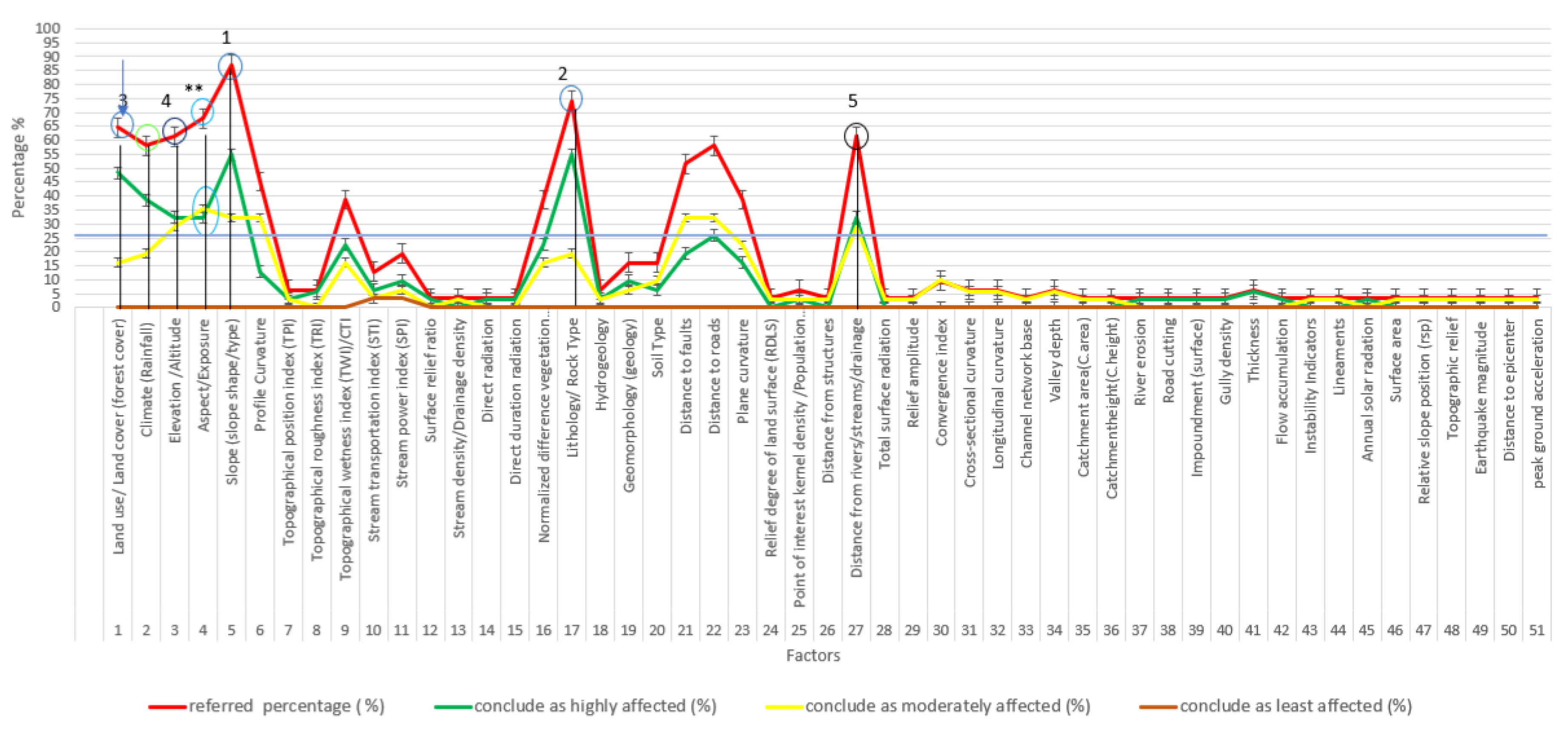
Figure 4.
Earthquakes occurred in WP and TP.
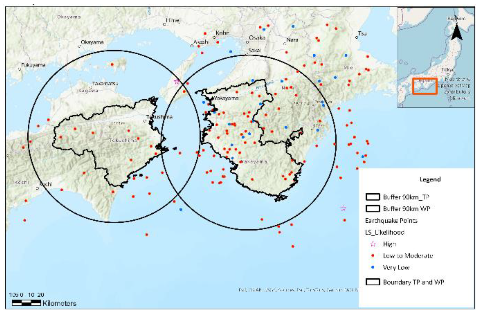
Figure 5.
Distribution of Variable Importance when Model is under training.
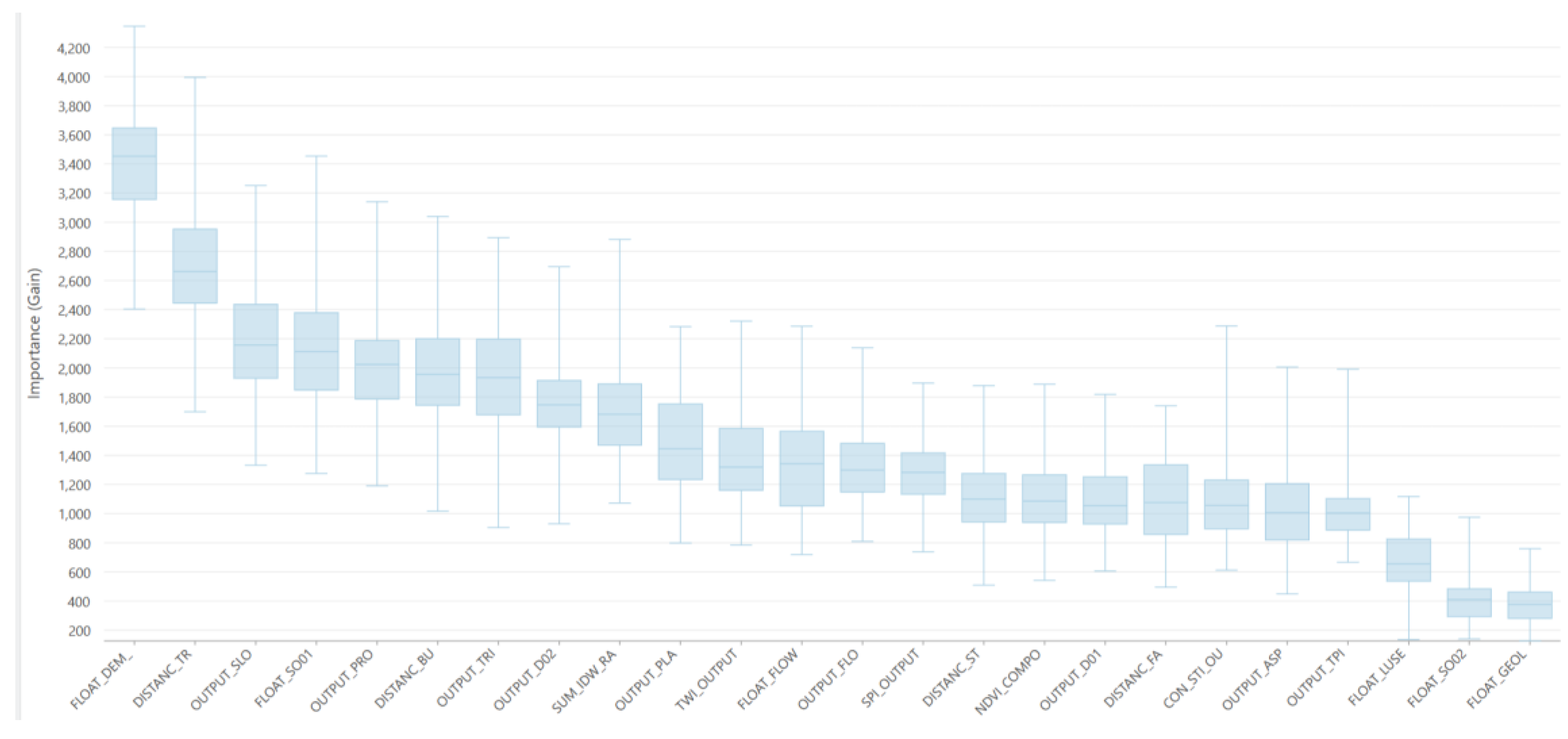
Figure 6.
Methodology Flow Chart (TP; Tokushima Prefecture, KD; Kegalle District).
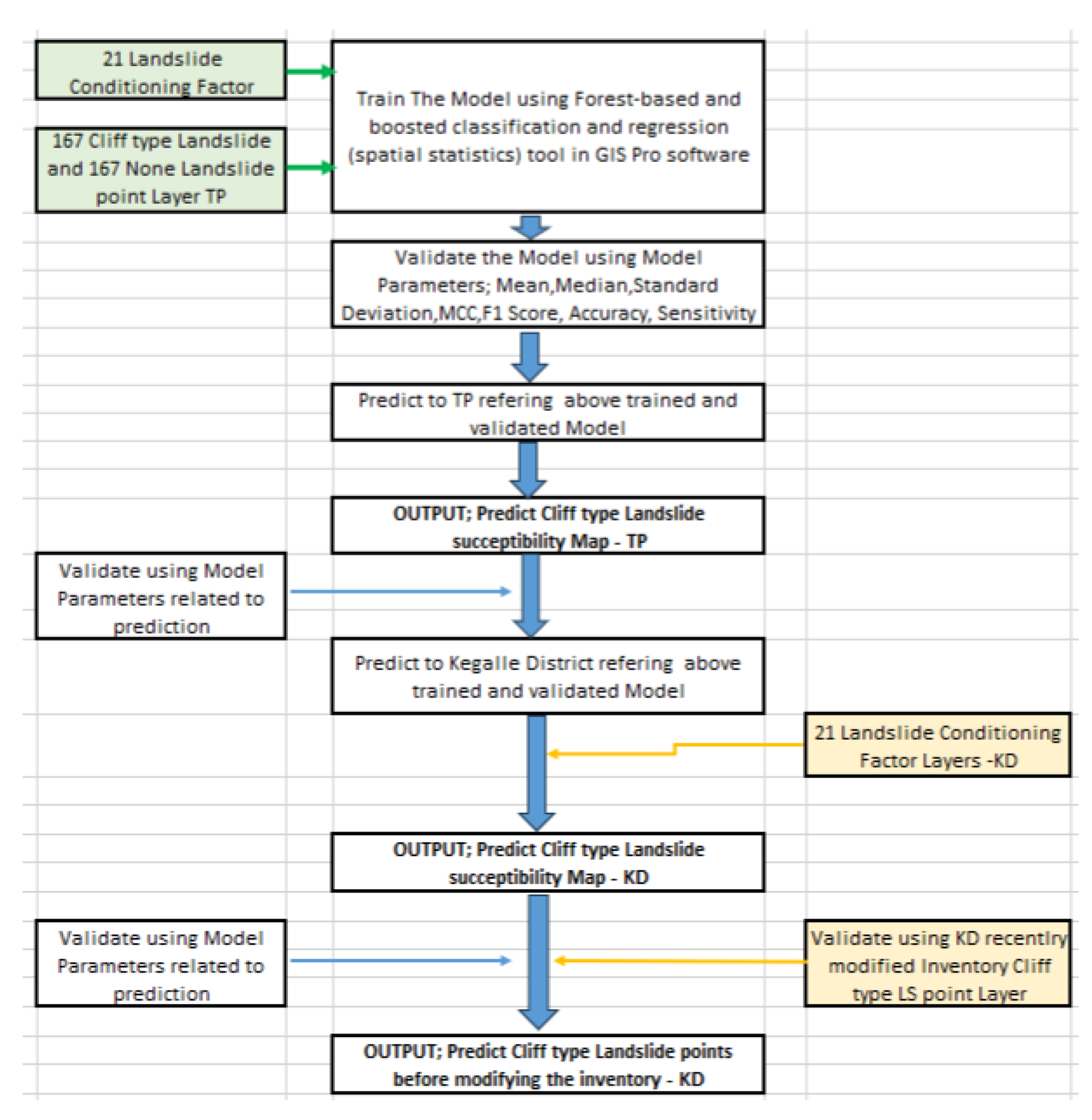

Table 1.
Elevation and Annual average rainfall ranges in Study Area (SA) and Reference Area (RA).
| Study/Reference Area | Elevation Range | Rainfall Range |
|---|---|---|
| Kegalle District (KD) | 10-1929 m | 167-452 mm/yr |
| Wakayama Prefecture | 0-1369 m | 120-333 mm/yr |
| Tokushima Prefecture | 0-1949 m | 125-287 mm/yr |
Table 2.
Data type and data collection sources.
| Landslide Conditioning Factor | Kegalle District | Tokushima and Wakayama Pref. |
|---|---|---|
| Land use, Road, Structures, waterbodies | Survey Dept. | MLIT website [11] |
| Geology, Fault | Geological Survey and Mines Bureau | MLIT website [11] |
| Rainfall | Meteorological department | AMeDAS website [3] |
| Soil type | ISRIC World soil information website [23] | MLIT website [11] |
Table 3.
Number of landslides in each inventory.
| SA /RA | All Types of LS Points | Cliff/Slope Failure LS Points |
|---|---|---|
| KD | 214 | Not specified before modifying the inventory |
| WP | 641 | 535 |
| TP | 260 | 167 – To create and train the Model |
Disclaimer/Publisher’s Note: The statements, opinions and data contained in all publications are solely those of the individual author(s) and contributor(s) and not of MDPI and/or the editor(s). MDPI and/or the editor(s) disclaim responsibility for any injury to people or property resulting from any ideas, methods, instructions or products referred to in the content. |
© 2025 by the authors. Licensee MDPI, Basel, Switzerland. This article is an open access article distributed under the terms and conditions of the Creative Commons Attribution (CC BY) license (http://creativecommons.org/licenses/by/4.0/).
Copyright: This open access article is published under a Creative Commons CC BY 4.0 license, which permit the free download, distribution, and reuse, provided that the author and preprint are cited in any reuse.


