
Submitted:
10 July 2025
Posted:
11 July 2025
You are already at the latest version
Abstract
Methane (CH4) is known as the most potent greenhouse gas in the short term. With the growing urgency of mitigating climate change and monitoring methane emissions, many emerging satellite systems have been launched in the past decade to observe methane and other greenhouse gases from space. These satellites are either capable of pinpointing and quantifying super emitters or deriving regional emissions with a more frequent revisit time. This study aims to reconcile emissions estimated from point source satellites and those from regional mapping satellites, and to investigate the potential of integrating point-based quantification and regional-based quantification techniques. To do that, we quantified methane emissions from the Permian Basin separately by applying the divergence method to the TROPOMI Level-2 data product, as well as an event-based approach using CH₄ plumes quantified by Carbon Mapper systems. The resulted annual CH₄ emissions estimates from the Permian Basin in 2024 are 1.83 ± 0.96 Tg and 1.26 [0.78, 2.02] Tg for divergence and event-based methods, respectively. The divergence-based emissions estimate shows a more comprehensive spatial distribution of emissions across the Permian Basin, whereas the event-based approach highlights the grid cells with the short-duration super-emitters. The emissions from grids with detectable emissions under both methods show strong agreement (R²≈0.642). After substituting the overlap cells’ values from divergence-based emissions estimation with those from event-based estimation, the combined emissions estimate is 2.68 [1.88, 3.54] Tg, which is reconciled with Permian Basin emissions estimates from previous studies. We found that CH₄ emissions from the Permian Basin have been gradually reduced over the past five years. Furthermore, this case study indicates the potential for integrating estimations from both methods to generate a more comprehensive regional emissions estimate.
Keywords:
methane emissions
; satellite emissions observations
; reconciliation
; point plume detection
; regional quantification
; emissions from permian basin
; annual emissions estimation
; emissions event
1. Introduction
Over the past decade, the adoption of low Earth orbit (LEO) satellites to measure and quantify methane (CH4) emissions has garnered significant attention (Jacob et al., 2022). Satellite data have become an important source to pinpoint the global super-emitters, reveal regional emissions, evaluate emissions benchmarks, and help the government to develop policy towards mitigating global warming and achieving the net-zero goal (Bi & Suresh Neethirajan, 2024; Chen et al., 2023; Cusworth et al., 2024; Irakulis-Loitxate et al., 2021; Irakulis-Loitxate et al., 2022; Liu et al., 2021; Maasakkers et al., 2022; MacLean et al., 2024; Thorpe et al., 2023). The rapid growth of applications has been largely facilitated by advancements in retrieval techniques, which, in turn, have driven the deployment of numerous satellites explicitly designed for dedicated monitoring of CH4 and other Greenhouse Gases (GHGs) (e.g., GHGSats, MethaneSat, and Tanager-1). Retrievals of the column-average CH4 mixing ratio in the atmosphere require observing short-wave infrared (SWIR) radiation with frequencies ranging from 1.63 to 1.70 µm or 2.2 to 2.4 µm (Jacob et al., 2022). Therefore, several launched satellites equipped with instruments that are also capable of detecting wavelengths sensitive to atmospheric CH4 (e.g., Sentinel-2, Landsat-8).
Based on the spatial resolution of satellite observations, satellite systems can be classified as point-source detectors and regional mappers (Jacob et al., 2022). Point-source detectors, such as GHGSats, Worldview-3, EMIT, GESat, Sentinel-2, PRISMA, and Tanager-1, can pinpoint and quantify exact emission sources at the site-level on the ground, such as waste treatment plants, coal mines, oil and gas facilities, landfills, and other industrial sites (Cusworth et al., 2024; Dogniaux et al., 2024; Guanter et al., 2021; Irakulis-Loitxate et al., 2022; MacLean et al., 2024; Pandey et al., 2019; Thorpe et al., 2023). The detection and quantification of several point-source detectors have already been verified in the past single-blind test study (Sherwin et al., 2023). Conversely, observations from regional mappers such as Sentinel-5P TROPOMI, ENVISAT-SCIAMACHY, and GOSAT have a lower spatial resolution but can usually quantify emissions from entire basins or countries (Chen et al., 2022; Li et al., 2023; Liu et al., 2024; Liu et al., 2021; Lu et al., 2021; Maasakkers et al., 2019; Qu et al., 2021; Wecht et al., 2014; Zhang et al., 2020). Furthermore, the newly launched MethaneSat can estimate both regional emissions and pinpoint CH4 plumes at the site level (EDF, 2024; South, 2024). Although some studies have also successfully identified the source using a regional mapper (de Foy et al., 2023; Lauvaux et al., 2022; Schuit et al., 2023; Xing et al., 2024). However, only the super-emitter can be detected due to the high minimum detection limit of regional mappers (Dubey et al., 2023).
The performance of satellite systems is influenced by various atmospheric factors, including aerosol optical thickness, surface albedo, solar altitude, cloud cover, topographic roughness, and wind speed (Gao et al., 2023; Finman, 2024). Some of these variables, such as persistent cloud cover and low solar altitude, systematically affect observations in high-latitude regions and areas near the equator (Gao et al., 2023). While it is still premature to consider satellite observations the silver bullet solution, they provide valuable information across most high-emission regions globally and significantly reduce the temporal coverage gaps of the majority of anthropogenic emissions sources, particularly by integrating images from multiple satellites.
The finalized methane emissions data product from satellite systems typically includes either a retrieved CH4 concentration or mixing ratio map (also known as a level 2 data product) or regional quantification results (also known as a level 3 data product) or isolated CH4 plume with visualization and associated quantification results (also known as a level 4 data product). Each type of data product supports different methods for estimating methane emissions, depending on the scale of detail (regional scale vs site scale) in the observations. The common quantification methods for point-source detectors include inverse Gaussian plume model (e.g., de Foy et al., 2023), mass balance (e.g., Buchwitz et al., 2017), integrated mass enhancement (e.g., Thorpe et al., 2023), and machine learning-based method (e.g., Joyce et al., 2023). For regional mappers, systematic quantification methods, such as Integrated Methane Inversion (IMI; Estrada et al., 2025; Varon et al., 2022), as well as divergent methods, have been widely adopted over the past five years (Liu et al., 2024; Liu et al., 2021).
Previous studies have found a discrepancy in emission estimates between top-down (TD) and bottom-up (BU) approaches (e.g., Vaughn et al., 2018; Zavala-Araiza et al., 2015; Zhao et al., 2023). However, discrepancies can also exist between the two different TD approaches, such as those between point-source detectors and regional mappers. In this study, we present a reconciliation between regional emission estimates from regional mappers and aggregated plume-level quantifications from point-source detectors. Specifically, we apply the event-based methodology developed by Gao et al. (2025), incorporating plume data published by Carbon Mapper and the divergence method developed by Liu et al. (2021) with the TROPOMI Level-2 data product and CAMS EAC4 reanalysis dataset to separately estimate emissions from the Permian Basin, US, for 2024. To ensure the singularity of the emission source sector and sufficient observational coverage, we selected Permian Basin BU estimation from the Global Fuel Exploitation Inventory (GFEI) 3.0 (Scarpelli et al., 2019) and previous CH4 emissions investigation results from Permian Basin as references.
2. Materials and Methods
2.1. Study Area
The Permian Basin is the most productive oil and gas (O&G) basin in the United States (EIA, 2024), located in West Texas and southeastern New Mexico (see Figure 1a). Over the past five years, the Permian Basin has been consistently monitored and identified as the highest CH4-emitting O&G region in the country (Irakulis-Loitxate et al., 2021; Liu et al., 2021; Varon et al., 2022; Zhang et al., 2020). For the divergence method, we estimate emissions for the entire Texas and the southeast corner of New Mexico. For the event-based method, we defined an extended study area (red highlighted region in Figure 1a) that encompasses the boundary of the Permian Basin, specifically, from 29 to 34.5 degrees north and -105.5 to -99.5 degrees west.
2.2. Regional Methane Emission Estimate – The Divergence Method
2.2.1. TROPOMI Level 2 Data Product
The TROPOspheric Monitoring Instrument (TROPOMI) onboard the Sentinel-5 Precursor satellite relies on passive remote sensing to measure atmospheric constituents, including CH4. RemoTeC full-physics algorithm was applied to retrieve the atmospheric CH4 total column (or concentrations) from Earth radiance measurements in the near-infrared (NIR, 675 nm to 775 nm) and shortwave infrared (SWIR, 2305 nm – 2385 nm) spectral bands (Hu et al., 2016; Lorente et al., 2021). The TROPOMI Level 2 data product provides daily observations of the column-mean dry air mixing ratio of CH4 (XCH4) across Texas, comprising 13 or 14 orbits of data (Landgraf et al., 2023). To correct the underestimation of the TROPOMI XCH4 data for low albedo, bias-corrected XCH4 is also provided in the data product. The pixel size of the image product is approximately 7 km × 5.5 km for data collected after August 6, 2019. In this study, quality-assured TROPOMI level 2 XCH4 observations (i.e., qa_value ≥ 0.5) from January 1, 2024, to December 31, 2024, were used for basin-level emission estimates via the divergence method.
2.2.2. Reanalysis Data from CAMS EAC4
To perform the divergent method developed by Liu et al. (2021), atmospheric variables, including surface pressure, level-specific methane column, the u and v wind components, were extracted from the ECMWF Atmospheric Composition Reanalysis 4 (EAC4; Copernicus Atmosphere Monitoring Service, 2020). Different from the spatial resolution of TROPOMI XCH4 observations, the spatial resolution of EAC4 data is 0.75° × 0.75° (Inness et al., 2019). The EAC4 model does not rely on prior CH4 emissions from bottom-up inventories such as the Emissions Database for Global Atmospheric Research (EDGAR) 8.0 or the Global Fuel Exploitation Inventory (GFEI) v3. As a result, the distribution of CH4 columns is primarily influenced by atmospheric transport and orography (Liu et al., 2024).
2.2.3. The Divergence Method
Figure 2 illustrates the detailed emissions estimation workflow developed by Liu et al. (2021). Equations and procedural steps are provided in Appendix A. The divergence method comprises three primary steps. First, we used the high-pass median filter to destrip and correct the bias caused by the satellite’s viewing angle (Liu et al., 2021). Second, we calculated the average daily divergence using Eq.1. We downloaded the vertical column of CH4 above PBL (), as well as u- and v-wind components () at the PBL from EAC4 (PBL is approximately 500 meters above the surface, corresponding to model level 53 in EAC4). The and are total columns of methane and dry air density used to retrieve TROPOMI’s column-mean dry air mixing ratio of CH4, which can be directly assessed from TROPOMI Level 2 data product. To ensure that EAC4 data (0.75° × 0.75°) matches our predefined 0.25° grid cells, we downsampled the EAC4 data using bilinear interpolation (Kirkland, 2010). Next, we calculated the daily CH4 mixing ratio below the PBL () using Eq.2, as well as the regional background () of each grid cell using the lower 10 percentile of three surrounding cells (7 by 7 grid cells window). Then, the daily divergence () can be calculated by multiplying the CH4 enhancement (i.e., the daily mixing ratio minus the regional background, ) by the air density column in the PBL ().
and
This calculation was repeated for each day. Note that a single day may include more than one image (observation). To avoid underestimation (Roberts et al., 2023), we first averaged the emissions divergence () within each day and then averaged across all days to calculate the daily mean emissions for each grid cell (). Finally, we applied a linear regression between emissions divergence and background divergence following the approach of Liu et al. (2024) to generate the final emissions estimates (see Eq. A6 in Appendix A).
2.3. Event-Based Methane Emissions Estimate
2.3.1. Methane Plumes from Carbon Mapper
Carbon Mapper (https://carbonmapper.org/data) is a non-profit organization that publishes CH4 and CO2 plumes detected by both airborne systems (Airborne Visible/Infrared Imaging Spectrometer–Next Generation [AVIRIS-NG], Global Airborne Observatory [GAO]) and satellite systems (EMIT, International Space Station [ISS], and Tanager-1), along with associated quantification results and source information (Duren et al., 2025). Figure 1b shows a sample plume published on Carbon Mapper’s data portal. Several types of data products are available for download on the portal. In this study, we downloaded Level 4 products, which include plumes and sources, from both airborne and satellite platforms, covering the period from January 1, 2024, to December 31, 2024. Quantification results, uncertainty estimates, plume IDs, detection times, and plume coordinates from the L4A–Plume Emissions product, as well as source coordinates, plume IDs, scene IDs, observation scene names, and persistence from the L4B–Source Emissions product, were used for event creation in this study (Carbon Mapper, 2025).
2.3.2. Event Creation
Figure 2 also presents the overall workflow for estimating regional emissions by aggregating discrete emission events. By utilizing emissions plumes and sources published by Carbon Mapper, we constructed emissions events using an event-based framework developed by Gao et al. (2025). According to the definition, only partially resolved events (PREs) are created in this study, which represent events measured using remote sensing technologies and require an estimated duration based on non-detections (i.e., the observations from aircraft and satellite systems conclude that no emissions are detected from the given source). The other two types of events are resolved events (RE), in which durations are determined using operational data, and unresolved events (UE), which are either not being measured or below the detection limit of the remote sensing technology. Table A1 provides the definitions and descriptions of three types of events. Figure 3 illustrates an example of creating PRE using plume detection and non-detect data from Carbon Mapper systems.
Each emissions source on the ground can have multiple events that occur throughout the year, and each event has a finite number of detections and non-detections. Therefore, we can bookend each plume detection by using its proceeding and succeeding null-detections. The null-detections can be derived by accessing the plume name and scene name of each source for which the scene name does not relate to the plume is defined as a null-detection. When multiple plumes share the same null detections, we conclude that they represent the same event by following Allen’s interval algebra (Allen, 1983). When there are no null detections, the first and last day of the year will be used to bind the event. Thus, the succeeding and proceeding null detections ( and ) are 2024-01-01T00:00:00 and 2024-12-31T23:59:59 for 2024. Furthermore, the event rate () is calculated by averaging the rates of all plumes included in the event. The difference between and is the observed duration. By combining the persistence (i.e., number of plume detection days [] divided by the number of observation days []; Carbon Mapper, 2025) and observed duration, the estimated event duration of each PRE () can be calculated by using equation as follows:
and the total emissions of event can be calculated by using Eq.4.
2.3.3. Calculate Event-Based Emissions
We applied total Eq.5 (Gao et al., 2025) to calculate the total emissions from all events of a given source.
Where , and indicates the number of resolved, partially resolved, and unresolved events, respectively. The , , and represents total CH4 emissions from a given resolved, partially resolved, and unresolved events, respectively. Since operational data are not available. We only considered emissions from PREs and UEs in this study.
For each source, total emissions from PREs were calculated straightforwardly aggregating all emissions from PRE calculated using Eq.4. However, we need additional two steps to calculate emissions from UEs.
First, we derive distributions for the expected emission rate, event duration, and probability of occurrence based on the constructed PREs. The consolidated rate and duration of PREs usually follow right-skewed distributions, which mathematically can be expressed using exponential function (see Eq.6). Additionally, the likelihood of event occurrence () for a given year can be approximately equal to the ratio between the number of detected plumes (plumes count) and number of observation attempts (scene count), which also can be expressed using exponential function.
Where is either the rate or duration or probability of event occurrence sampled under the probability , and and are parameters required to fit different distributions
where is the mean and is standard deviation of rate or duration or probability of event occurrence.
Therefore, we use a log-normal probability density function (PDF; Eq.7) to fit the empirically measured distributions of event rate (), duration (), and probability of event occurrence (). The optimal and are used to create the expected rate (), duration (), and probability of event occurrence () distributions.
Second, we applied Monte Carlo approach to extrapolate emissions of UEs per each source (Gao et al., 2025). The Monte Carlo simulation begins by setting the timestamp to the start time of the simulation (2024-01-01T00:00:00) and initializing emissions from UEs () to 0 kg. For each source, the simulation proceeds hourly and sample a from . Based on sampled , we calculate the likelihood of no event occurrence () can be calculated by using 1 - . Then a binomial distribution (with outcome of 0 or 1) can be created by using and . Next, we sample from the constructed binomial distribution. If an emission occurs, the emission rate () and duration () are sampled from the and , respectively. The then updated by adding the emissions calculated from multiplying and , and the simulation time is incremented by . If no emission event occurs, the simulation time advances by one hour. This process is repeated until the end of the simulation time (2024-12-31T23:59:59). The of a source is calculated by summing emissions from all sampled UEs. The simulation is repeated for 105 iterations, and the median (), along with the 2.5th and 97.5th percentiles of the distribution, are calculated to represent the simulated emissions from UEs and their associated uncertainty.
Finally, we calculate grid emissions () by aggregating of all point sources within each 0.25° grid cell (Eq.7).
3. Results and Discussion
3.1. Divergence of Methane Emissions
Figure 4a illustrates the TROPOMI days (i.e., the number of days that TROPOMI have valid level 2 data) throughout 2024. The median number of TROPOMI days in our study region in 2024 is 140 days. By focusing on the Permian Basin, the median and average TROPOMI days are 184 days and 182 days, respectively. For 2024, the mean XCH4 in the Permian Basin was 1917.12 ± 6.28 ppb (see Figure 4b). The concentration hotspots in the Permian Basin are located near the central Midland and the central Delaware Basins (highlighted in Figure 4b). The calculated divergence of CH4 emissions using Eq.4 ranged from –15.11 to 16.60 kg/km2/hour prior to applying the linear regression correction (Figure 4c). The uncorrected divergence from hotspot grid cells near the Midland Basin was lower than that of grid cells in the Delaware Basin.
After the correction, the CH4 emission divergence was adjusted to a range of 0 to 16.6 kg/km2/hour (Figure 4d). By multiplying the area and normalizing it with the number of hours per year, we converted the calculated emissions per unit area and time into annual emissions estimates. As shown in Figure 4e, the total calculated CH4 emissions of the Permian Basin were 1.83 Tg for the year 2024. Approximately 15% of grid cells contributed to 83.6% of the total emissions (~1.53 Tg) within the Basin. The mean CH4 emissions across all grid cells within the Permian Basin were 0.007 Tg, and the maximum CH4 emissions were 0.097 Tg. We also applied the Monte Carlo approach developed by Liu et al. (2024) to calculate the uncertainties associated with the estimated emissions. As indicated in Figure 4f, uncertainties of emissions per grid cell ranged from 44.51% to 167.10%. We calculated the root mean square error to represent the overall uncertainties in basin-level emissions estimation. Finally, our estimate for the Permian Basin for 2024 was 1.83 ± 0.96 Tg.
3.2. Event-Based Methane Emissions
A total of 1,465 plumes and 656 sources were downloaded from the Carbon Mapper data portal. After aggregating the plumes and sources to our predefined 0.25° grid cells, the number of plumes per grid cell ranged from 0 to 228, with an average of 28 and a median of 6 plumes, respectively (Figure 5a). Similarly, the number of sources per grid cell ranged from 0 to 84, with an average of 13 and a median of 5 (Figure 5b).
Following the event-based framework proposed by Gao et al. (2025), we constructed 565 partial resolved events (PREs) by combining plume and scene information from the source data. As shown in Figure 5c, the number of PREs per grid cell ranged from 1 to 90, with an average of 14 and a median of 3 events per grid cell. Figures 6a to 6c also show that the majority of plumes, sources, and constructed events were located near the Texas-New Mexico border, indicating the spatial observation coverage of the Carbon Mapper satellite systems.
Using the constructed events, we created the best-fit curves for event rate, duration, and occurrence probability distributions (Figures 6d, 6e, and 6f). The mean and standard deviation for the event rate were 5.54 and 1.11, respectively, while those for the event duration were 6.42 and 2.48. The yielded best-fit parameters (a and b) are 0.000072 and –0.0006 for the rate and 0.0424 and –0.0004 for the duration. Similarly, the mean and standard deviation for emission event probability were –1.81 and 0.69, respectively, and the fitted exponential function parameters were a = 7.1 and b = –6.09. These curves were used to generate expected distributions and simulate UEs.
Figure 6.
event-based emissions estimations map for (a) only PREs and (b) both PREs and UEs. The highlighted region in (b) indicates the Delaware Basin of the Permian Basin.
Figure 6.
event-based emissions estimations map for (a) only PREs and (b) both PREs and UEs. The highlighted region in (b) indicates the Delaware Basin of the Permian Basin.
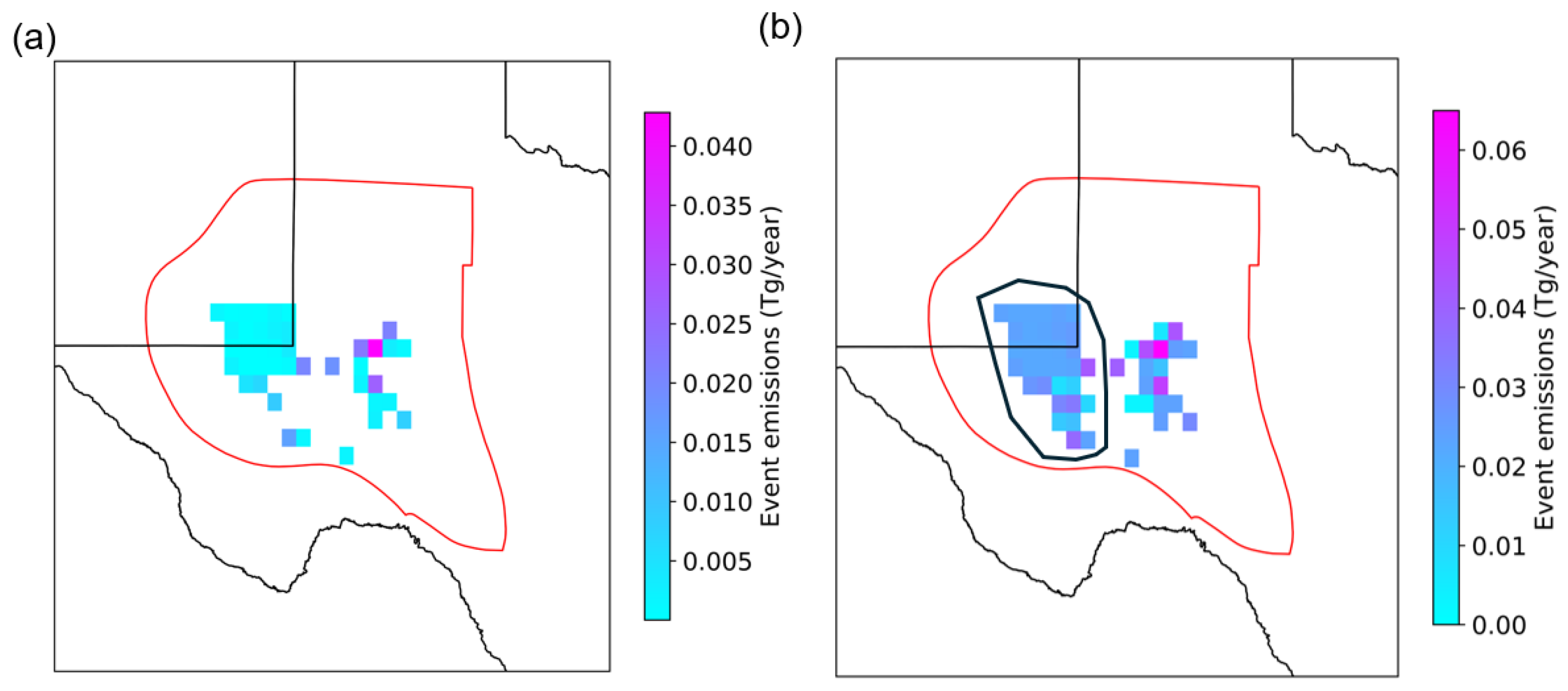
Figure 6a shows the map of estimated emissions aggregated from only PREs. The total methane emissions in 2024 from only constructed PREs were estimated at 0.23 Tg, with a 95% confidence interval (CI) of [0.19, 0.27] Tg. Although the majority of Carbon Mapper plumes and sources were observed near the Texas-New Mexico border, the grid cells with the highest emissions (~0.043 Tg) from PREs were located in the central Midland basin. After incorporating simulated emissions from UEs (as shown in Figure 6b), the total estimated emissions for the Permian Basin increased to 1.26 Tg, with a 95% confidence interval of [0.78, 2.02] Tg. The Delaware Basin was highlighted from the simulation of UEs. In total, 1.03 Tg of previously unobserved emissions were simulated across 52 grid cells based on locations of published sources from Carbon Mapper. Emissions of grid cells near the northern Delaware Basin (i.e., border between New Mexico and Texas) increased significantly after adding emissions from UEs, ranging from 0.002 to 0.03 Tg.
3.3. Reconciliation
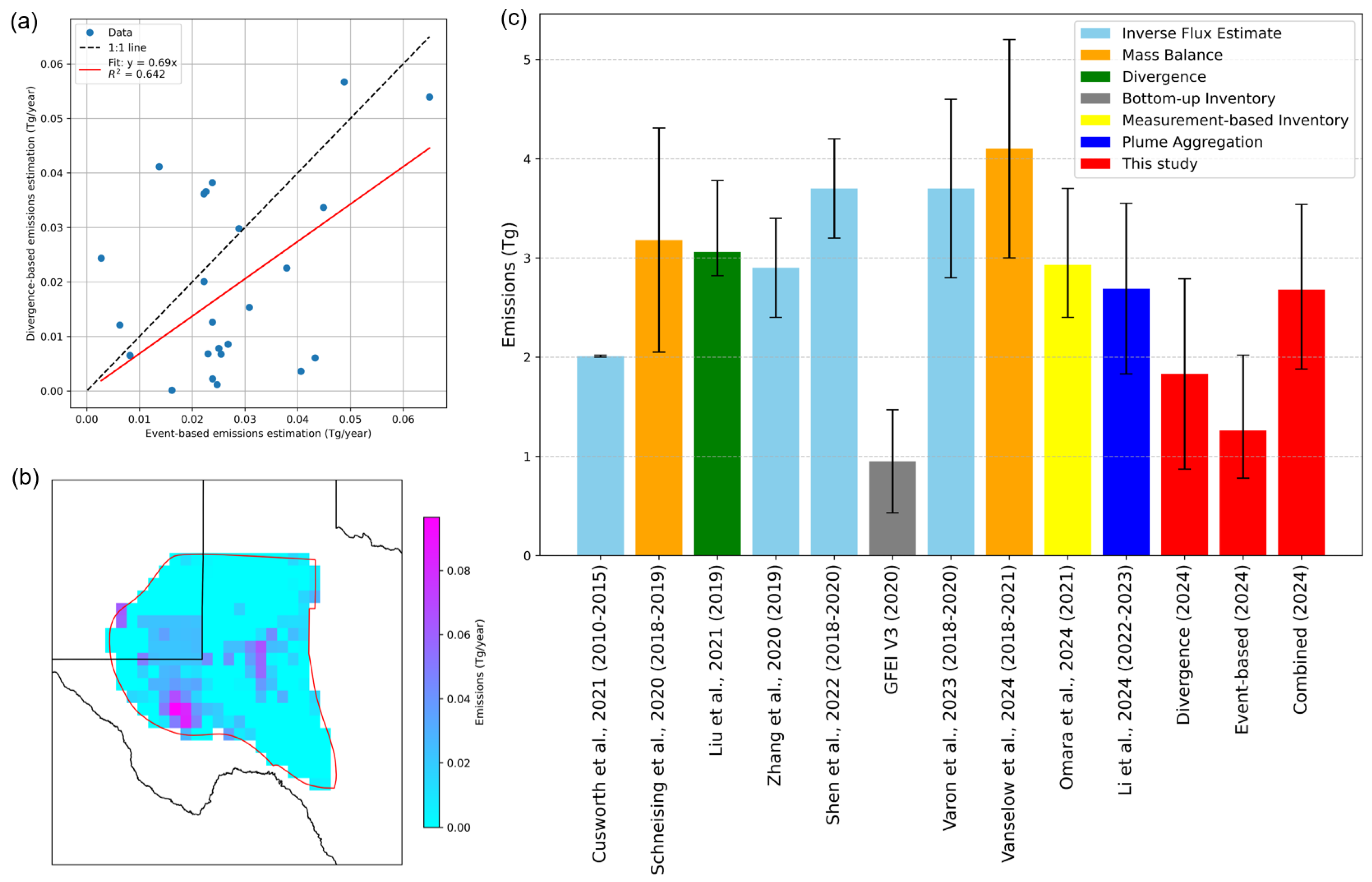
Since the event-based method only estimates emissions where Carbon Mapper has detected sources, only 52 grid cells within the Permian Basin have event-based emissions estimates. Among them, 26 grid cells were found with emissions under the divergence method. We then further compared the grid-specific emissions from both methods. The mean and median differences of these 26 grid cells were 0.016 Tg and 0.015 Tg. The robust linear regression analysis reveals a strong positive correlation between emissions estimates from 26 grid cells that are available from the results of both methods (see Figure 7a). The total emissions estimated by the two methods were generally comparable (1.83 ± 0.96 Tg vs 1.26 [0.78 Tg, 2.02 Tg]). Although emissions estimated using the event-based method were 0.57 Tg lower than those estimated using the divergence method, the uncertainty ranges of both estimates overlapped, with a 31.1% discrepancy, indicating agreement within statistical bounds.
A key limitation of the event-based method is its inability to estimate emissions in grid cells where no detectable emissions are present (i.e., emissions below ~100 kgCH4/hr). However, this method is particularly effective at capturing short-duration, high-emission events that may be smoothed out or missed in the time-averaged divergence-based approaches. For example, as shown in Figure 4e, the New Mexico portion of the Delaware Basin was not highlighted using the divergence method alone.
To leverage the strengths of both approaches, we integrated the event-based estimates with the divergence-based regional estimates by substituting divergence-based values with event-based estimates in 26 grid cells where plume-derived results were available (see Figure 7b). By doing so, it is reasonable to believe the divergence-based emission estimate was corrected to include the instantaneous high emission events. This hybrid approach yielded a total CH4 emission estimate of 2.68 Tg for the Permian Basin, with a 95% confidence interval of [1.88, 3.54] Tg.
We compared the integrated emission estimate with previous methane emission studies conducted between 2015 and 2023, as well as the bottom-up inventory provided in GFEI V3 (Scarpelli et al., 2025). A summary of referenced studies is provided in Table A2 of Appendix B. The inversion-based emissions estimates, which rely on atmospheric transport models (e.g., GEOS-Chem) and prior emission information such as bottom-up inventories or source maps (e.g., Zhang et al., 2020; Varon et al., 2023), often serve as a benchmark for other methods (e.g., Liu et al., 2021). Past TROPOMI-based inverse flux estimates for the Permian Basin range from 2.9 ± 0.5 Tg/year (2019) to 3.7 ± 0.5 Tg/year (2020) (Zhang et al., 2020; Shen et al., 2022; Varon et al., 2023). In addition to inverse modeling, we compared our estimates with other techniques, including the divergence method (Liu et al., 2021), the Gaussian integral mass balance method (Schneising et al., 2020), the point-source aggregation method (Li et al., 2024), and a measurement-based inventory approach (Omara et al., 2024). These studies reported Permian Basin emissions as follows:
- 3.06 Tg [2.82, 3.78] for 2019 (Liu et al., 2021)
- 3.18 ± 1.13 Tg averaged over 2018–2019 (Schneising et al., 2020)
- 2.69 ± 0.86 Tg averaged over 2022–2023 (Li et al., 2024)
- 2.93 Tg [2.4, 3.7] for 2021 (Omara et al., 2024)
Our combined estimate aligns well with the results from previous studies. Our integrated estimate is comparable but slightly lower than the previous estimates. Considering the reported decreasing trend of methane emissions from the Permian Basin (Varon et al., 2023; Sherwin et al., 2025), it is reasonable to expect lower methane emissions in 2024 compared to the emissions estimates derived in earlier periods.
We also found that the event-based estimate (1.26 Tg; 95% CI: [0.78, 2.02] Tg) was reconciled with the GFEI V3 bottom-up inventory (0.95 ± 0.52 Tg), which specifically focuses on the energy sector, respectively. This agreement provided further confidence in applying the event-based method to capture short-duration super emitters in regional emissions estimation.
Overall, the comparison of emissions estimates spanning 2018-2024 confirmed the decline of methane emissions in the Permian Basin. This downward trend suggests that the impact of regulatory efforts, operational improvements, and increased public and industry scrutiny has been evident over the past six years.
4. Conclusions
In conclusion, both the divergence-based and event-based methane emission approaches produce broadly consistent annual CH4 emissions estimates for the Permian Basin in 2024. The divergence method, using TROPOMI observations, yields a total emission estimate of approximately 1.83 ± 0.96 Tg. In contrast, the point-source event-based method, utilizing data from Carbon Mapper systems and Monte Carlo estimation for undetected emissions, estimates 1.26 Tg (95% CI: 0.78–2.02 Tg). By comparing overlapping grid cells where both methods produced estimates, the strong correlation (R2 ≈ 0.642) indicates the reconciled emissions estimates between the two methods.
Since the divergence method is based on daily averages, short-duration events within a day may be neglected. Therefore, the event-based method serves as a valuable complement by capturing short-duration super-emitter events using point-source data. The divergence-based emission estimate was then corrected by substituting divergence estimates with event-based values in the overlapping grid cells to include instantaneous high-emission events. The integrated estimate is 2.68 [1.88, 3.54] Tg and is close to the emission estimates derived from other approaches from previous studies.
Overall, this study demonstrates that point-source and regional satellite-based methods, though different in approach, can produce mutually consistent emission estimates when reconciled through the proposed methodology. Future research will focus on extending this comparison to multiple regions globally, evaluating the availability of emissions observations, and developing a streamlined workflow for combining both methods to advance methane emission estimates in regions lacking prior data.
Author Contributions
Conceptualization, M.G., and Z.X.; methodology, M.G., and Z.X.; data curation and formal analysis, M.G.; writing—original draft preparation, M.G.; writing—review and editing, M.G., and Z.X.; visualization, M.G.; All authors have read and agreed to the published version of the manuscript.
Data Availability Statement
The datasets used in this work are publicly accessible as follows: The TROPOMI Level 2 methane observations data products are available at: https://browser.dataspace.copernicus.eu/ (accessed on 20 March 2025); the CAMS ECMWF Atmospheric Composition Reanalysis 4 datasets are available at: https://www.copernicus.eu/en/access-data/copernicus-services-catalogue/cams-global-reanalysis-eac4 (accessed on 14 April 2025); and the Carbon Mapper Level 4 data product (methane plumes and sources) are available at: https://data.carbonmapper.org/#1.06/0/50.5 (accessed on 17 April 2025).
Acknowledgments
The authors thank the Carbon Mapper team for providing publicly accessible methane plume and source data through an easy-to-use data portal; the TROPOMI and Copernicus Data Space Ecosystem team for making the Level 2 data products publicly available; the SensorUp Inc. and GeoSensorWeb Lab for their contributions to the development of the emissions event framework and methodologies.
Conflicts of Interest
The authors declare no conflicts of interest.
Appendix A
There are three primary steps included in the divergence method, which are applying destriping technique to correct the TROPOMI Level 2 data product, calculating average daily divergence, and utilizing the linear regression to derive the corrected emissions estimation. The TROPOMI Level 2 data were corrected by using high-pass median filter both along across-track directions with four neighboring pixels and along the time direction with 50 previous obits and 50 succeeding orbits to remove the viewing angle bias (Liu et al., 2021). During the correction only the valid TROPOMI observations (the quality assurance value – qa_value > 0.5) are used.
For regional estimate, we used the divergent method proposed by Liu et al. (2021, 2024) and E. F. M. Koene et al. (2024) to quantify CH4 emissions. The method relies on continuity equation (Eq. A1) between divergence (), emission () and Sink () for steady state (Beirle et al., 2019).
On daily basis, divergence () in the planetary boundary layer (PBL) contains both background divergence () and emissions divergence (). Under the assumption of homogeneity, the can be ignored and the daily emissions divergence equals daily emissions. Therefore, Eq. A1 can be written as:
If we treat each grid cell as an emissions source, the of the grid cell is the divergence product of vertical CH4 column () and horizontal wind () of the grid cell. Thus Eq. A2 can be written as:
By following Liu et al. (2021, 2024), Eq. A3 can be further rewritten by calculating at PBL using daily methane enhancement (i.e., daily mixing ratio subtracts the regional background; ) times the air density column in the PBL () to eliminate the effects of orography and transport in upper atmosphere and calculate the daily mean emissions per each grid cell ().
and
Where and are total column of methane and dry air density used by the retrieval method of TROPOMI’s column-mean dry air mixing ratio of CH4. Both of these two variables can be accessed directly from the TROPOMI Level 2 data product. is the vertical column of CH4 above the PBL, which is downloaded from EAC4. In this study, we assume the height of PBL is approximately 500 meters, corresponding to model level 53 (ECMWF, 2024). Thus, the vertical column of CH4 above the PBL can be calculated by summing column methane from level 1 to level 52. Similar to vertical column of CH4 above the PBL, the u- and v-component in the PBL are also downloaded from EAC4 at level 53 to calculate the horizontal wind. Next, the regional background () is calculated by averaging the background of each pixel. For each pixel, the background is calculated by using the lower 10 percentile of three surrounding pixels (7 by 7 pixels window). The regional background is only valid if more than ten grid cells with the 7 by 7 region are valid observations (Liu et al., 2024). To ensure EAC4 data matches our predefined 0.25° grid cells, we downsampled all data from EAC4 data by using bilinear interpolation (Kirkland, 2010). By repeating this process each day, we are able to calculate the daily divergence of emissions. Each day may contain more than one image (observation), before calculating the average divergence of emissions () using Eq. A4, we first averaging per each day and then across all day to avoid underestimation (Roberts et al., 2023).
Finally, we applied the linear regression between emdaydivergence and background divergence. The slope () and intercept () of fitted line are used to correct emission estimate by using the Eq. A6 if fitting is statistically significant (p-value < 0.01).
Appendix B

Table A1.
Three categories of emission event types.
| Emission Event Type | Definition | Duration Determination | Emissions Quantity from Events | Uncertainty |
|---|---|---|---|---|
| Resolved Event (RE) | Events with durations determined using operational data/log | Extracted from operational data/log | Calculated | Only quantification uncertainty is considered |
| Partially Resolved Event (PRE) | Events with duration that are either measured by remote sensing technologies or estimated using null-detection and rules | Simulated by using proceedings and succeeding null-detection times | Calculated | Quantification uncertainty and duration estimation uncertainty |
| Unresolved Event (UE) | Events that are missing from annual emissions data | Simulated | (1) Simulate emissions that are not detected using POD checks (2) Simulate emissions by random sample RE and PRE |
Estimated in the simulations |
Table A2.
A summary of previous satellite-based CH4 emissions studies in the Permian Basin.
| Authors | Year of investigation | Emission rate | Uncertainty | Method | Unit | doi |
|---|---|---|---|---|---|---|
| Cusworth et al., 2021 | 2010–2015 | 2.01 | 0.01 | GOSAT inverse flux estimate - derived from Maasakkers et al., 2021 | Mt yr−1 | 10.1038/s43247-021-00312-6 |
| Zhang et al., 2020 | 2018–2019 | 2.68 | 0.5 | TROPOMI inverse flux estimate - O&G production | Mt yr−1 | 10.1126/sciadv.aaz5120 |
| 2018–2019 | 2.9 | 0.5 | TROPOMI inverse flux estimate - basin total | Mt yr−1 | ||
| Shen et al., 2022 | 2018-2020 | 2.9 | 0.4 | TROPOMI inverse flux estimate | Mt yr−1 | 10.5194/acp-22-11203-2022 |
| 2018-2020 | 3.7 | 0.5 | TROPOMI inverse flux estimate with an adjusted prior | Mt yr−1 | ||
| Qu et al. 2021 | 2019 | 2.36 | GOSAT inverse flux estimate | Mt yr−1 | 10.5194/acp-21-14159-2021 | |
| 2019 | 2.43 | TROPOMI inverse flux estimate | Mt yr−1 | |||
| Liu et al., 2021 | 2019 | 3.06 | 2.82 - 3.78 | Divergence method: the continuity equation connecting the divergence (D), emission (E) and sink (S) for steady state. | Mt yr−1 | 10.1029/2021GL094151 |
| Schneising et al., 2020 | 2018-2019 | 3.18 | 1.13 | Gaussian integral mass balance method - TROPOMI/WFMD v1.2 | Mt yr−1 | 10.5194/acp-20-9169-2020 |
| Vanselow et al. 2024 | 2018-2021 | 4.1 | 1.1 | Automated detection of regions with persistently enhanced methane concentrations (TROPOMI) coupled with mass balance quantification method. | Mt yr−1 | 10.5194/acp-24-10441-2024 |
| Veefkind et al., 2023 | 2019 | 3.0 | 0.7 | Divergence method | Mt yr−1 | 10.1029/2022JD037479 |
| Varon et al., 2023 | 2018-2020 | 3.7 | 0.9 | Weekly TROPOMI inverse flux estimate | Mt yr−1 | 10.5194/acp-23-7503-2023 |
| Li et al., 2024 | 2022-2023 | 2.69 | 0.86 | Aggregation from GF-4 plume mapping | Mt yr−1 | 10.1029/2024JD040870 |
| Omara et al., 2024 | 2021 | 335 | 274-428 | Measurement-based methane emissions inventory (EI-ME) | t h−1 | 10.5194/essd-16-3973-2024 |
References
- Allen, J. F. (1983). Maintaining knowledge about temporal intervals. Communications of the ACM, 26(11), 832–843. [CrossRef]
- Bi, H., & Suresh Neethirajan. (2024). Satellite Data and Machine Learning for Benchmarking Methane Concentrations in the Canadian Dairy Industry. Sustainability, 16(23), 10400–10400. [CrossRef]
- Buchwitz, M., Schneising, O., Reuter, M., Heymann, J., Krautwurst, S., Bovensmann, H., Burrows, J. P., Boesch, H., Parker, R. J., Somkuti, P., Detmers, R. G., Hasekamp, O. P., Aben, I., Butz, A., Frankenberg, C., & Turner, A. J. (2017). Satellite-derived methane hotspot emission estimates using a fast data-driven method. Atmospheric Chemistry and Physics, 17(9), 5751–5774. [CrossRef]
- Bureau of Economic Geology. (2024). Permian Basin GIS Projects and Databases. Utexas.edu. https://www.beg.utexas.edu/resprog/permianbasin/gis.htm.
- Carbon Mapper. (2025). Product Guide: Data Definition & Specification. Carbonmapper.org. https://carbonmapper.org/articles/product-guide.
- Chen, Z., Jacob, D. J., Nesser, H., Sulprizio, M. P., Lorente, A., Varon, D. J., Lu, X., Shen, L., Qu, Z., Penn, E., & Yu, X. (2022). Methane emissions from China: a high-resolution inversion of TROPOMI satellite observations. Atmospheric Chemistry and Physics, 22(16), 10809–10826. [CrossRef]
- Chen, Z., Jacob, D., Gautam, R., Omara, M., Stavins, R. N., Stowe, R. C., Nesser, H., Sulprizio, M. P., Lorente, A., Varon, D. J., Lu, X., Shen, L., Qu, Z., Pendergrass, D. C., & Hancock, S. (2023). Satellite quantification of methane emissions and oil–gas methane intensities from individual countries in the Middle East and North Africa: implications for climate action. Atmospheric Chemistry and Physics, 23(10), 5945–5967. [CrossRef]
- Crippa, M., Guizzardi, D., Pagani, F., Marcello Schiavina, Melchiorri, M., Pisoni, E., Graziosi, F., Muntean, M., Maes, J., Dijkstra, L., Martin Van Damme, Lieven Clarisse, & Coheur, P. (2024). Insights into the spatial distribution of global, national, and subnational greenhouse gas emissions in the Emissions Database for Global Atmospheric Research (EDGAR v8.0). Earth System Science Data, 16(6), 2811–2830. [CrossRef]
- Cusworth, D. H., Bloom, A. A., Ma, S., Miller, C. E., Bowman, K., Yin, Y., Maasakkers, J. D., Zhang, Y., Scarpelli, T. R., Qu, Z., Jacob, D. J., & Worden, J. R. (2021). A Bayesian framework for deriving sector-based methane emissions from top-down fluxes. Communications Earth & Environment, 2(1), 1–8. [CrossRef]
- Cusworth, D. H., Duren, R. M., Ayasse, A. K., Jiorle, R., Howell, K., Aubrey, A., Green, R. O., Eastwood, M. L., Chapman, J. W., Thorpe, A. K., Heckler, J., Asner, G. P., Smith, M. L., Thoma, E., Krause, M. J., Heins, D., & Thorneloe, S. (2024). Quantifying methane emissions from United States landfills. Science (New York, N.Y.), 383(6690), 1499–1504. [CrossRef]
- de Foy, B., Schauer, J. J., Lorente, A., & Borsdorff, T. (2023). Investigating high methane emissions from urban areas detected by TROPOMI and their association with untreated wastewater. Environmental Research Letters, 18(4), 044004. [CrossRef]
- Dogniaux, M., Maasakkers, J., Girard, M., Jervis, D., McKeever, J., Schuit, B., Sharma, S., Lopez-Noreña, A., Varon, D., & Aben, I. (2024). Satellite survey sheds new light on global solid waste methane emissions. Earth Arxiv. [CrossRef]
- Dubey, L., Cooper, J., & Hawkes, A. (2023). Minimum detection limits of the TROPOMI satellite sensor across North America and their implications for measuring oil and gas methane emissions. Science of the Total Environment, 872, 162222. [CrossRef]
- Duren, R., Cusworth, D., Ayasse, A., Howell, K., Diamond, A., Scarpelli, T., Kim, J., O’neill, K., Lai-Norling, J., Thorpe, A., Zandbergen, S. R., Shaw, L., Keremedjiev, M., Guido, J., Giuliano, P., Goldstein, M., Nallapu, R., Barentsen, G., Thompson, D. R., & Roth, K. (2025). The Carbon Mapper emissions monitoring system. [CrossRef]
- EDF. (2024). Environmental Defense Fund - MethaneSAT - Earth Engine Data Catalog . https://developers.google.com/earth-engine/datasets/publisher/edf-methanesat-ee.
- EIA. (2024). Drilling Productivity Report. https://www.eia.gov/petroleum/drilling/archive/2024/05/pdf/dpr-full.pdf.
- Estrada, L. A., Varon, D. J., Sulprizio, M., Nesser, H., Chen, Z., Balasus, N., Hancock, S. E., He, M., East, J. D., Mooring, T. A., Alonso, A. O., Maasakkers, J. D., Aben, I., Baray, S., Bowman, K. W., Worden, J. R., Cardoso-Saldaña, F. J., Reidy, E., & Jacob, D. J. (2025). Integrated Methane Inversion (IMI) 2.0: an improved research and stakeholder tool for monitoring total methane emissions with high resolution worldwide using TROPOMI satellite observations. Geoscientific Model Development, 18(11), 3311–3330. [CrossRef]
- Finman, L. (2024). Satellites are no silver bullet for methane monitoring. Nature, 636(8042), 275–275. [CrossRef]
- Gao, M., Xing, Z., Vollrath, C., Hugenholtz, C. H., & Barchyn, T. E. (2023). Global observational coverage of onshore oil and gas methane sources with TROPOMI. Scientific Reports, 13(1), 16759. [CrossRef]
- Guanter, L., Irakulis-Loitxate, I., Gorroño, J., Sánchez-García, E., Cusworth, D. H., Varon, D. J., Cogliati, S., & Colombo, R. (2021). Mapping methane point emissions with the PRISMA spaceborne imaging spectrometer. Remote Sensing of Environment, 265, 112671. [CrossRef]
- Hu, H., Hasekamp, O., Butz, A., Galli, A., Landgraf, J., Aan de Brugh, J., Borsdorff, T., Scheepmaker, R., & Aben, I. (2016). The operational methane retrieval algorithm for TROPOMI. Atmospheric Measurement Techniques, 9(11), 5423–5440. [CrossRef]
- Inness, A., Ades, M., Agustí-Panareda, A., Barré, J., Benedictow, A., Blechschmidt, A.-M., Dominguez, J. J., Engelen, R., Eskes, H., Flemming, J., Huijnen, V., Jones, L., Kipling, Z., Massart, S., Parrington, M., Peuch, V.-H., Razinger, M., Remy, S., Schulz, M., & Suttie, M. (2019). The CAMS reanalysis of atmospheric composition. Atmospheric Chemistry and Physics, 19(6), 3515–3556. [CrossRef]
- Irakulis-Loitxate, I., Guanter, L., Liu, Y.-N., Varon, D. J., Maasakkers, J. D., Zhang, Y., Chulakadabba, A., Wofsy, S. C., Thorpe, A. K., Duren, R. M., Frankenberg, C., Lyon, D. R., Hmiel, B., Cusworth, D. H., Zhang, Y., Segl, K., Gorroño, J., Sánchez-García, E., Sulprizio, M. P., & Cao, K. (2021). Satellite-based survey of extreme methane emissions in the Permian basin. Science Advances, 7(27). [CrossRef]
- Irakulis-Loitxate, I., Guanter, L., Maasakkers, J. D., Zavala-Araiza, D., & Aben, I. (2022). Satellites Detect Abatable Super-Emissions in One of the World’s Largest Methane Hotspot Regions. Environmental Science & Technology, 56(4), 2143–2152. [CrossRef]
- Jacob, D. J., Varon, D. J., Cusworth, D. H., Dennison, P. E., Frankenberg, C., Gautam, R., Guanter, L., Kelley, J., McKeever, J., Ott, L. E., Poulter, B., Qu, Z., Thorpe, A. K., Worden, J. R., & Duren, R. M. (2022). Quantifying methane emissions from the global scale down to point sources using satellite observations of atmospheric methane. Atmospheric Chemistry and Physics, 22(14), 9617–9646. [CrossRef]
- Joyce, P., Ruiz Villena, C., Huang, Y., Webb, A., Gloor, M., Wagner, F. H., Chipperfield, M. P., Barrio Guilló, R., Wilson, C., & Boesch, H. (2023). Using a deep neural network to detect methane point sources and quantify emissions from PRISMA hyperspectral satellite images. Atmospheric Measurement Techniques, 16(10), 2627–2640. [CrossRef]
- Kirkland, E. J. (2010). Bilinear Interpolation. Springer EBooks, 261–263. [CrossRef]
- Landgraf , J., Lorente, A., Langerock, B., & Sha, M. K. (2023). S5P Mission Performance Centre Methane [L2__CH4___] Readme. https://sentinels.copernicus.eu/documents/247904/3541451/Sentinel-5P-Methane-Product-Readme-File.
- Lauvaux, T., Giron, C., Mazzolini, M., d’Aspremont, A., Duren, R., Cusworth, D., Shindell, D., & Ciais, P. (2022). Global assessment of oil and gas methane ultra-emitters. Science, 375(6580), 557–561. [CrossRef]
- Li, F., Bai, S., Lin, K., Feng, C., Sun, S., Zhao, S., Wang, Z., Zhou, W., Zhou, C., & Zhang, Y. (2024). Satellite-Based Surveys Reveal Substantial Methane Point-Source Emissions in Major Oil & Gas Basins of North America During 2022–2023. Journal of Geophysical Research Atmospheres, 129(19). [CrossRef]
- Li, S., Wang, C., Gao, P., Zhao, B., Jin, C., Zhao, L., He, B., & Xue, Y. (2023). High-Spatial-Resolution Methane Emissions Calculation Using TROPOMI Data by a Divergence Method. Atmosphere, 14(2), 388–388. [CrossRef]
- Liu, M., van der A, R., van Weele, M., Bryan, L., Eskes, H., Veefkind, P., Liu, Y., Lin, X., de Laat, J., & Ding, J. (2024). Current potential of CH4 emission estimates using TROPOMI in the Middle East. Atmospheric Measurement Techniques, 17(17), 5261–5277. [CrossRef]
- Liu, M., van der A, R., van Weele, M., Eskes, H., Lu, X., Veefkind, P., de Laat, J., Kong, H., Wang, J., Sun, J., Ding, J., Zhao, Y., & Weng, H. (2021). A New Divergence Method to Quantify Methane Emissions Using Observations of Sentinel-5P TROPOMI. Geophysical Research Letters, 48(18). [CrossRef]
- Lorente, A., Borsdorff, T., Butz, A., Hasekamp, O., aan de Brugh, J., Schneider, A., Wu, L., Hase, F., Kivi, R., Wunch, D., Pollard, D. F., Shiomi, K., Deutscher, N. M., Velazco, V. A., Roehl, C. M., Wennberg, P. O., Warneke, T., & Landgraf, J. (2021). Methane retrieved from TROPOMI: improvement of the data product and validation of the first 2 years of measurements. Atmospheric Measurement Techniques, 14(1), 665–684. [CrossRef]
- Lu, X., Jacob, D. J., Zhang, Y., Maasakkers, J. D., Sulprizio, M. P., Shen, L., Qu, Z., Scarpelli, T. R., Nesser, H., Yantosca, R. M., Sheng, J., Andrews, A., Parker, R. J., Boesch, H., Bloom, A. A., & Ma, S. (2021). Global methane budget and trend, 2010–2017: complementarity of inverse analyses using in situ (GLOBALVIEWplus CH4 ObsPack) and satellite (GOSAT) observations. Atmospheric Chemistry and Physics, 21(6), 4637–4657. [CrossRef]
- Maasakkers, J. D., Jacob, D. J., Sulprizio, M. P., Scarpelli, T. R., Nesser, H., Sheng, J.-X., Zhang, Y., Hersher, M., Bloom, A. A., Bowman, K. W., Worden, J. R., Janssens-Maenhout, G., & Parker, R. J. (2019). Global distribution of methane emissions, emission trends, and OH concentrations and trends inferred from an inversion of GOSAT satellite data for 2010–2015. Atmospheric Chemistry and Physics, 19(11), 7859–7881. [CrossRef]
- Maasakkers, J. D., Varon, D. J., Elfarsdóttir, A., McKeever, J., Jervis, D., Mahapatra, G., Pandey, S., Lorente, A., Borsdorff, T., Foorthuis, L. R., Schuit, B. J., Tol, P., van Kempen, T. A., van Hees, R., & Aben, I. (2022). Using satellites to uncover large methane emissions from landfills. Science Advances, 8(32). [CrossRef]
- MacLean, J.-P. W., Girard, M., Jervis, D., Marshall, D., McKeever, J., Ramier, A., Strupler, M., Tarrant, E., & Young, D. (2024). Offshore methane detection and quantification from space using sun glint measurements with the GHGSat constellation. Atmospheric Measurement Techniques, 17(2), 863–874. [CrossRef]
- Omara, M., Himmelberger, A., MacKay, K., Williams, J. P., Benmergui, J., Sargent, M., Wofsy, S. C., & Gautam, R. (2024). Constructing a measurement-based spatially explicit inventory of US oil and gas methane emissions (2021). Earth System Science Data, 16(9), 3973–3991. [CrossRef]
- Pandey, S., Gautam, R., Houweling, S., van der Gon, H. D., Sadavarte, P., Borsdorff, T., Hasekamp, O., Landgraf, J., Tol, P., van Kempen, T., Hoogeveen, R., van Hees, R., Hamburg, S. P., Maasakkers, J. D., & Aben, I. (2019). Satellite observations reveal extreme methane leakage from a natural gas well blowout. Proceedings of the National Academy of Sciences, 116(52), 26376–26381. [CrossRef]
- Qu, Z., Jacob, D. J., Shen, L., Lu, X., Zhang, Y., Scarpelli, T. R., Nesser, H., Sulprizio, M. P., Maasakkers, J. D., Bloom, A. A., Worden, J. R., Parker, R. J., & Delgado, A. L. (2021). Global distribution of methane emissions: a comparative inverse analysis of observations from the TROPOMI and GOSAT satellite instruments. Atmospheric Chemistry and Physics, 21(18), 14159–14175. [CrossRef]
- Roberts, C., Rutger IJzermans, Randell, D., Jones, M., Jonathan, P., Mandel, K., Hirst, B., & Shorttle, O. (2023). Avoiding methane emission rate underestimates when using the divergence method. Environmental Research Letters, 18(11), 114033–114033. [CrossRef]
- Scarpelli, T. R., Roy, E., Jacob, D. J., Sulprizio, M. P., Tate, R. D., & Cusworth, D. H. (2025). Using new geospatial data and 2020 fossil fuel methane emissions for the Global Fuel Exploitation Inventory (GFEI) v3. [CrossRef]
- Schneising, O., Buchwitz, M., Reuter, M., Vanselow, S., Bovensmann, H., & Burrows, J. P. (2020). Remote sensing of methane leakage from natural gas and petroleum systems revisited. Atmospheric Chemistry and Physics, 20(15), 9169–9182. [CrossRef]
- Schuit, B. J., Maasakkers, J. D., van, Mahapatra, G., Van, Pandey, S., Lorente, A., Borsdorff, T., Sander Houweling, Varon, D. J., McKeever, J., Jervis, D., Girard, M., Itziar Irakulis-Loitxate, Gorroño, J., Guanter, L., Cusworth, D. H., & Aben, I. (2023). Automated detection and monitoring of methane super-emitters using satellite data. Atmospheric Chemistry and Physics, 23(16), 9071–9098. [CrossRef]
- Shen, L., Gautam, R., Omara, M., Zavala-Araiza, D., Maasakkers, J. D., Scarpelli, T. R., Lorente, A., Lyon, D., Sheng, J., Varon, D. J., Nesser, H., Qu, Z., Lu, X., Sulprizio, M. P., Hamburg, S. P., & Jacob, D. J. (2022). Satellite quantification of oil and natural gas methane emissions in the US and Canada including contributions from individual basins. Atmospheric Chemistry and Physics, 22(17), 11203–11215. [CrossRef]
- Sherwin, E. D., Rutherford, J. S., Chen, Y., Aminfard, S., Kort, E. A., Jackson, R. B., & Brandt, A. R. (2023). Single-blind validation of space-based point-source detection and quantification of onshore methane emissions. Scientific Reports, 13(1), 3836. [CrossRef]
- Sherwin, E., Kruguer, J., Wetherley, E. B., Yakovlev, P. V., Brandt, A., Deiker, S., ... & Biraud, S. Comprehensive Aerial Surveys Find a Reduction in Permian Basin Methane Intensity from 2020-2023. Available at SSRN 5087216.
- South, D. W. (2024). Methane Emissions, Nowhere to Hide from Detection and Compliance Monitoring with Newly Launched Satellite. Climate and Energy, 40(11), 28–32. [CrossRef]
- Thorpe, A. K., Green, R. O., Thompson, D. R., Brodrick, P. G., Chapman, J. W., Elder, C. D., Itziar Irakulis-Loitxate, Cusworth, D. H., Ayasse, A. K., Duren, R. M., Frankenberg, C., Guanter, L., Worden, J. R., Dennison, P. E., Roberts, D. A., K. Dana Chadwick, Eastwood, M. L., Fahlen, J. E., & Miller, C. E. (2023). Attribution of individual methane and carbon dioxide emission sources using EMIT observations from space. Science Advances, 9(46). [CrossRef]
- Vanselow, S., Schneising, O., Buchwitz, M., Reuter, M., Bovensmann, H., Boesch, H., & Burrows, J. P. (2024). Automated detection of regions with persistently enhanced methane concentrations using Sentinel-5 Precursor satellite data. Atmospheric Chemistry and Physics, 24(18), 10441–10473. [CrossRef]
- Varon, D. J., Jacob, D. J., Hmiel, B., Gautam, R., Lyon, D. R., Omara, M., Sulprizio, M., Shen, L., Pendergrass, D., Nesser, H., Qu, Z., Barkley, Z. R., Miles, N. L., Richardson, S. J., Davis, K. J., Pandey, S., Lu, X., Lorente, A., Borsdorff, T., & Maasakkers, J. D. (2023). Continuous weekly monitoring of methane emissions from the Permian Basin by inversion of TROPOMI satellite observations. Atmospheric Chemistry and Physics, 23(13), 7503–7520. [CrossRef]
- Varon, D. J., Jacob, D. J., Sulprizio, M., Estrada, L. A., Downs, W. B., Shen, L., Hancock, S. E., Nesser, H., Qu, Z., Penn, E., Chen, Z., Lu, X., Lorente, A., Tewari, A., & Randles, C. A. (2022). Integrated Methane Inversion (IMI 1.0): a user-friendly, cloud-based facility for inferring high-resolution methane emissions from TROPOMI satellite observations. Geoscientific Model Development, 15(14), 5787–5805. [CrossRef]
- Varon, D. J., McKeever, J., Jervis, D., Maasakkers, J. D., Pandey, S., Houweling, S., Aben, I., Scarpelli, T., & Jacob, D. J. (2019). Satellite Discovery of Anomalously Large Methane Point Sources From Oil/Gas Production. Geophysical Research Letters, 46(22), 13507–13516. [CrossRef]
- Vaughn, T. L., Bell, C. S., Pickering, C. K., Schwietzke, S., Heath, G. A., Pétron, G., Zimmerle, D. J., Schnell, R. C., & Nummedal, D. (2018). Temporal variability largely explains top-down/bottom-up difference in methane emission estimates from a natural gas production region. Proceedings of the National Academy of Sciences, 115(46), 11712–11717. [CrossRef]
- Veefkind, J. P., R. Serrano-Calvo, J. de Gouw, Dix, B., O. Schneising, Buchwitz, M., J. Barré, van, Liu, M., & P.F. Levelt. (2023). Widespread Frequent Methane Emissions From the Oil and Gas Industry in the Permian Basin. Journal of Geophysical Research: Atmospheres, 128(3). [CrossRef]
- Wecht, K. J., Jacob, D. J., Frankenberg, C., Jiang, Z., & Blake, D. R. (2014). Mapping of North American methane emissions with high spatial resolution by inversion of SCIAMACHY satellite data. Journal of Geophysical Research: Atmospheres, 119(12), 7741–7756. [CrossRef]
- Xing, Z., Barchyn, T. E., Vollrath, C., Gao, M., & Hugenholtz, C. (2024). Satellite-Derived Estimate of City-Level Methane Emissions from Calgary, Alberta, Canada. Remote Sensing, 16(7), 1149. [CrossRef]
- Zavala-Araiza, D., Lyon, D. R., Alvarez, R. A., Davis, K. J., Harriss, R., Herndon, S. C., Karion, A., Kort, E. A., Lamb, B. K., Lan, X., Marchese, A. J., Pacala, S. W., Robinson, A. L., Shepson, P. B., Sweeney, C., Talbot, R., Townsend-Small, A., Yacovitch, T. I., Zimmerle, D. J., & Hamburg, S. P. (2015). Reconciling divergent estimates of oil and gas methane emissions. Proceedings of the National Academy of Sciences, 112(51), 15597–15602. [CrossRef]
- Zhang, Y., Gautam, R., Pandey, S., Omara, M., Maasakkers, J. D., Sadavarte, P., Lyon, D., Nesser, H., Sulprizio, M. P., Varon, D. J., Zhang, R., Houweling, S., Zavala-Araiza, D., Alvarez, R. A., Lorente, A., Hamburg, S. P., Aben, I., & Jacob, D. J. (2020). Quantifying methane emissions from the largest oil-producing basin in the United States from space. Science Advances, 6(17), eaaz5120. [CrossRef]
- Zhao, Y., Saunois, M., Bousquet, P., Lin, X., Hegglin, M. I., Canadell, J. G., Jackson, R. B., & Zheng, B. (2023). Reconciling the bottom-up and top-down estimates of the methane chemical sink using multiple observations. Atmospheric Chemistry and Physics, 23(1), 789–807. [CrossRef]
Figure 1.
(a) Spatial extent of the Permian Basin and our study area in the context of Texas and New Mexico, US; (b) the example of a published plume from the Carbon Mapper Data portal (https://carbonmapper.org/data).
Figure 1.
(a) Spatial extent of the Permian Basin and our study area in the context of Texas and New Mexico, US; (b) the example of a published plume from the Carbon Mapper Data portal (https://carbonmapper.org/data).
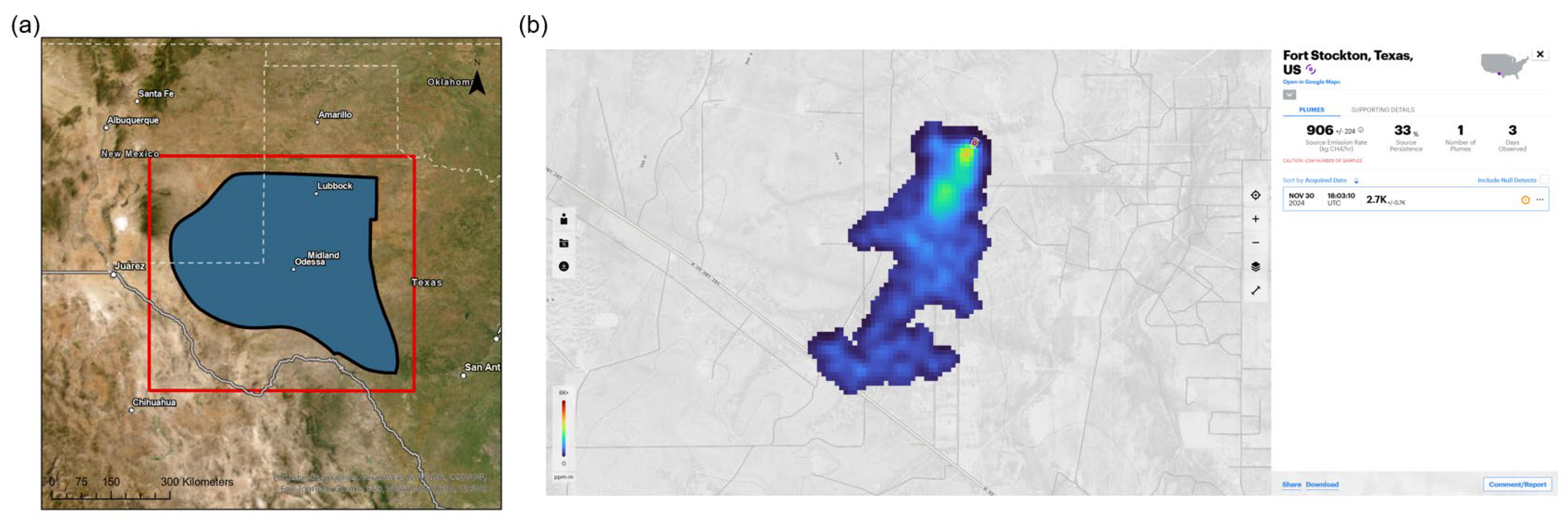
Figure 2.
Overview of the workflows for separately estimating emissions using the divergence and event-based methods in this study.
Figure 2.
Overview of the workflows for separately estimating emissions using the divergence and event-based methods in this study.
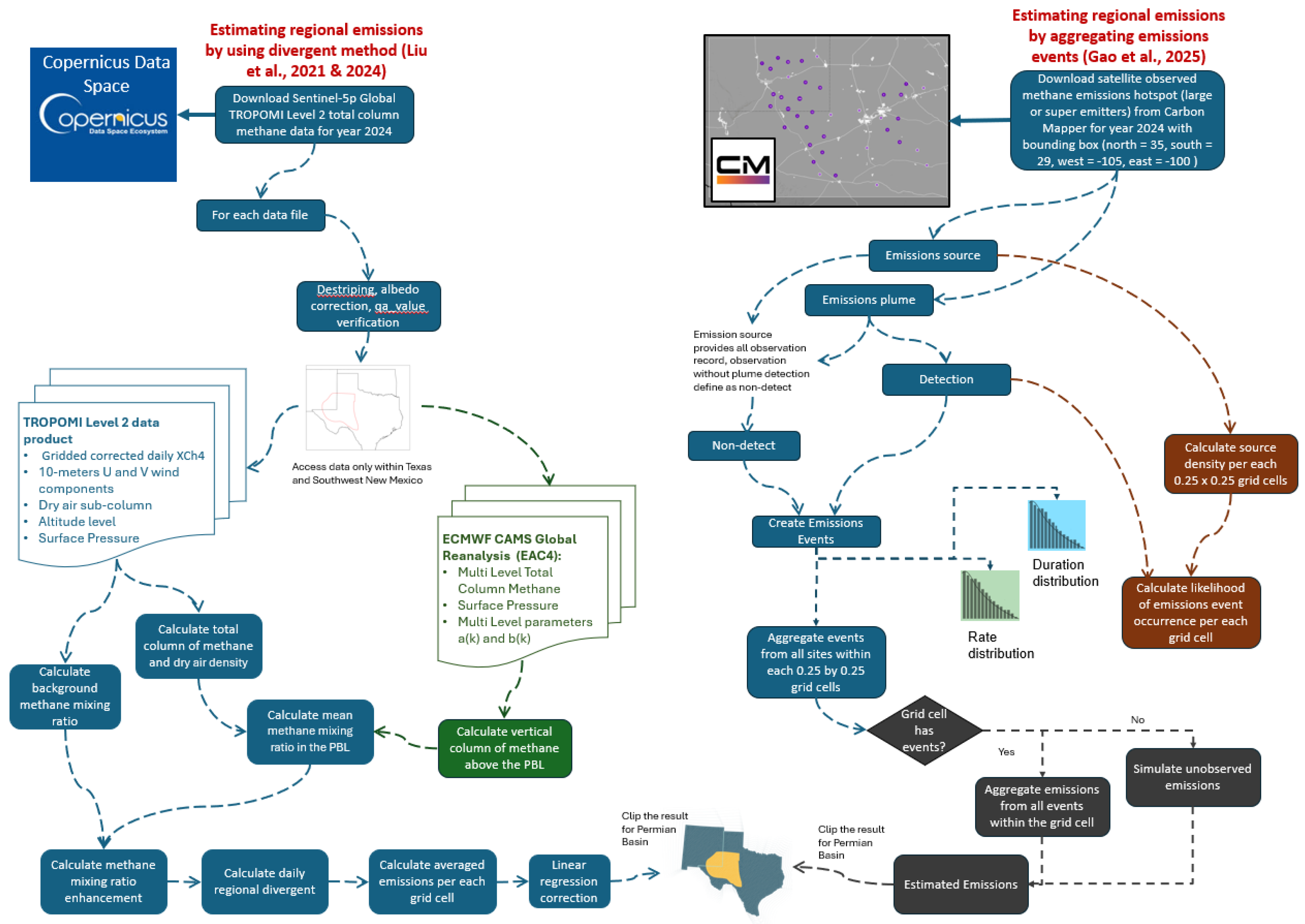
Figure 3.
An example of an emissions event constructed for a source (persistence equals 0.25) observed by Carbon Mapper systems. This source includes observations from two satellite systems: EMIT and Tanager-1. The red squares indicate two detected plumes captured by EMIT, with the plume IDs annotated above each square as provided by Carbon Mapper. These two plumes can be created as an event with a start time equal to the first day of 2024 (2024-01-01T00:00:00) and the end time determined by using a subsequent null detection (yellow square), observed by EMIT on February 12, 2024 (2024-02-12T21:48:43) with scene ID: f93fd6e4-b91c-4b34-9e6a-78257f39bf80:emi20240212t214843p14025. The red error bars represent the emission rate bounds (2459.66 + 188.13 kg/hr) of the event: the upper bound corresponds to plume emi20240204t165003p11008-A, while the lower bound (2130.13 - 297.78 kg/hr) corresponds to emi20240127t195904p13008-B. Thus, the rate and duration of this event are 2,294.89 kg/hr and 263.45 hours (), respectively. Apart from the null detection used to constrain the event, all other null detections are also annotated with their respective scene IDs. A green square highlights a potential missing observation for this source. The event constructed from these observations is classified as an unresolved event (UE), as only one event could be created. To account for unmeasured emissions from UEs, emissions are simulated from February 12, 2024, through the end of the year.
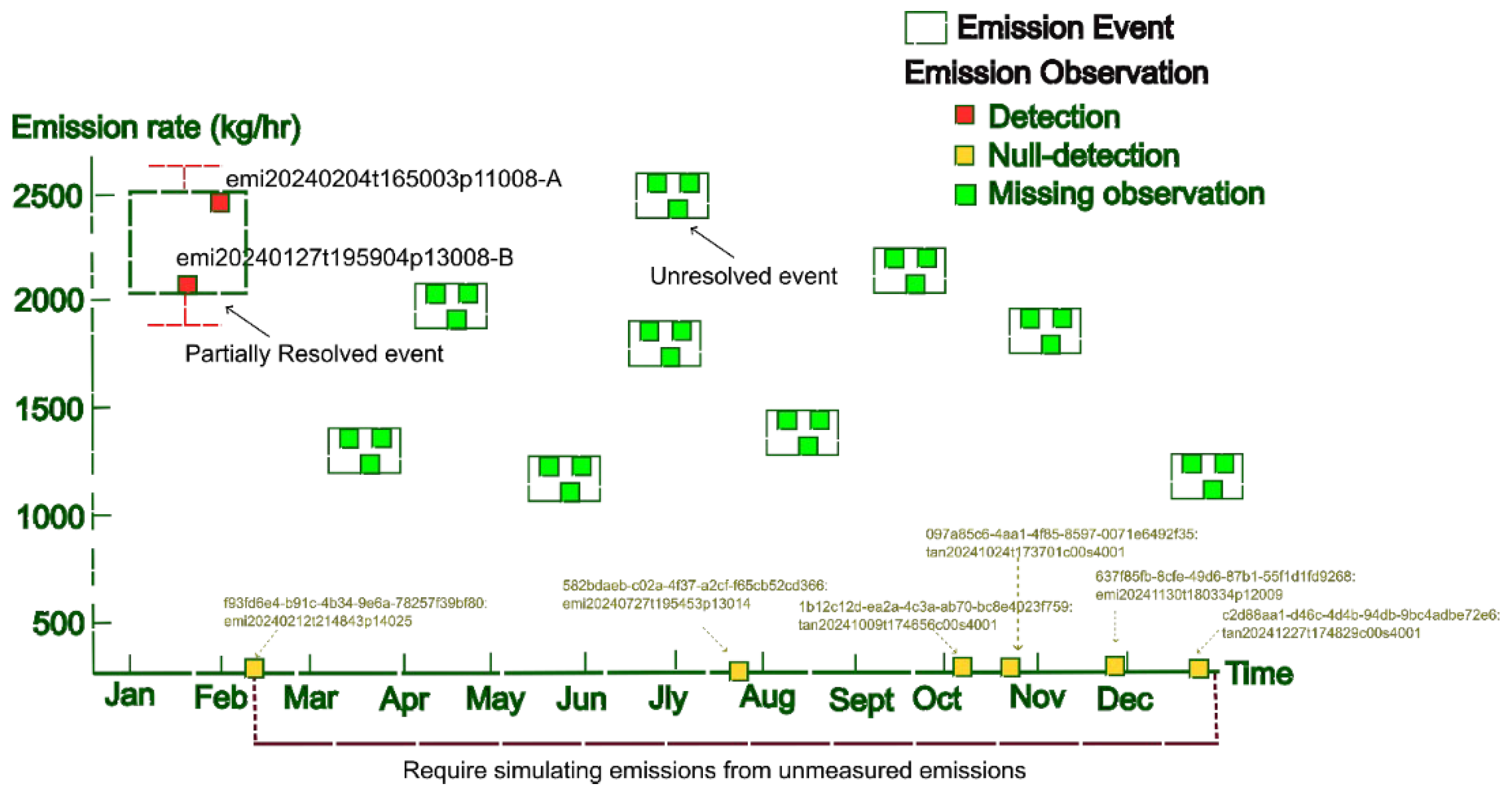
Figure 4.
The (a) TROPOMI observation days, (b) average CH4 methane mixing ratio, (c) average daily divergence of methane emissions before the linear regression, (d) average daily divergence of methane emissions after the linear regression, (e) annual emissions estimate, and (f) uncertainty of estimation of Permian Basin created by following the divergence estimation workflow. The red polygon represents the boundary of the Permian Basin downloaded from the shapefile posted by the Bureau of Economic Geology (2024). The green circle in (b) indicates the two CH4 concentration hotspots inside the Permian Basin, which are the central Midland and Delaware Basins.
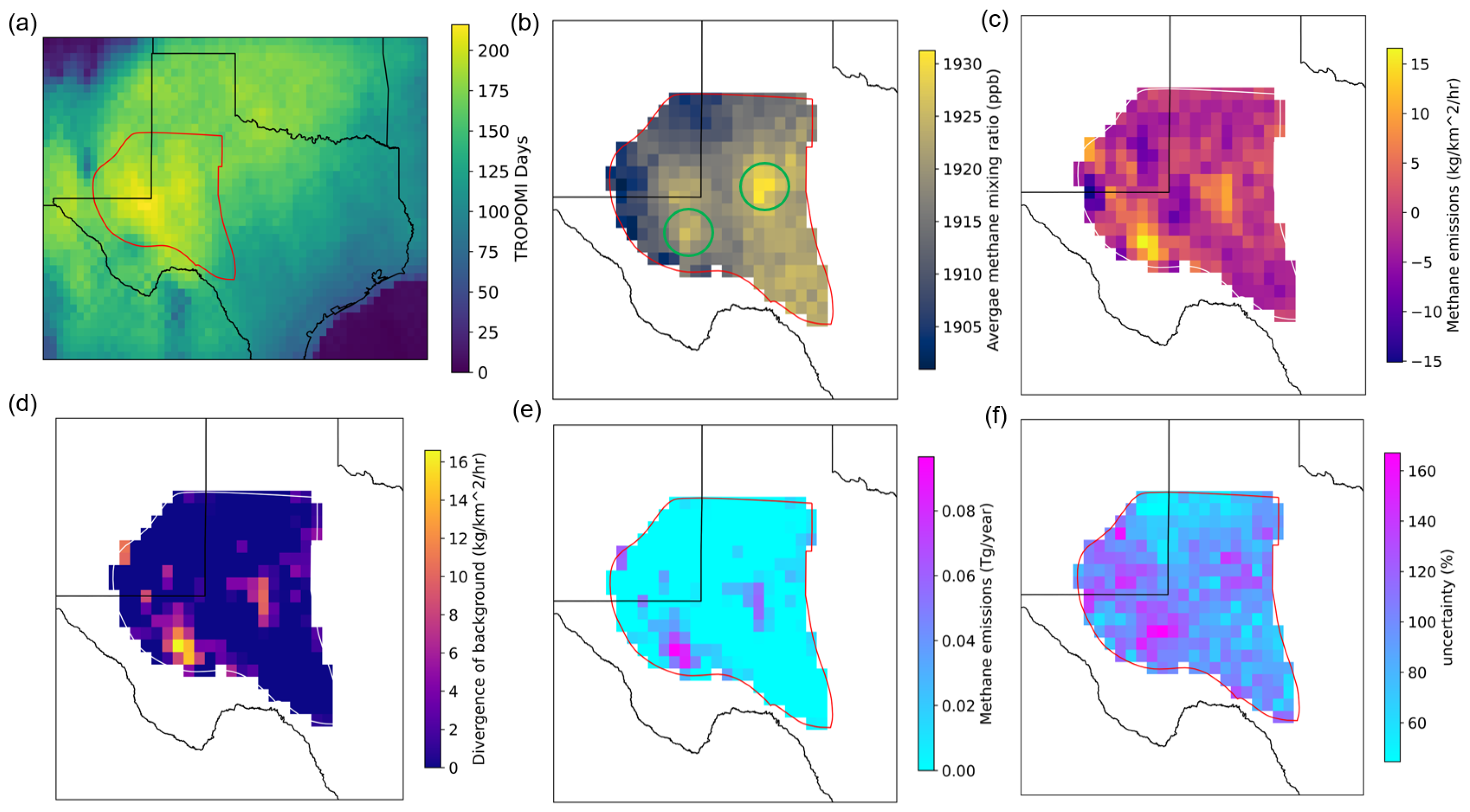
Figure 5.
The intermediate results from event creation. (a) The number of plumes per each 0.25° grid cell published by Carbon Mapper in Permian Basin for 2024; (b) The number of sources per each 0.25° grid cell published by Carbon Mapper in Permian Basin for 2024; (c) The number of events created per each 0.25° grid cell by following the event-based framework; (d) The fitting of event rate distribution; (e) The fitting of event duration distribution; and (f) The fitting of probability of event occurrence distribution.
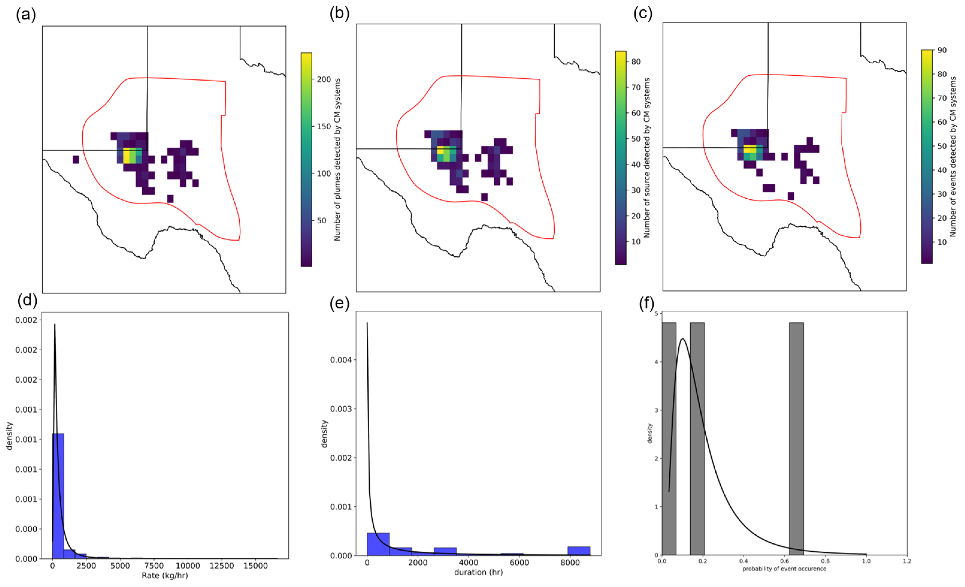
Figure 7.
The comparisons between the event-based and divergence methods. (a) the linear regression analysis between divergence-based emissions estimation and event-based emissions estimation; (b) The regional emissions estimate after combining results from both methods; and (c) The bar chart of total emissions from the Permian Basin among the event-based method, the divergence method, methane emissions from nine previous studies, the bottom-up inventory from GFEI V3 (2020), and emissions estimated using a combination of the event-based and divergence methods. The bars represent either the total emissions estimated for a particular year or the yearly average emissions derived from multi-year analyses. The error bars indicate the.
Disclaimer/Publisher’s Note: The statements, opinions and data contained in all publications are solely those of the individual author(s) and contributor(s) and not of MDPI and/or the editor(s). MDPI and/or the editor(s) disclaim responsibility for any injury to people or property resulting from any ideas, methods, instructions or products referred to in the content. |
© 2025 by the authors. Licensee MDPI, Basel, Switzerland. This article is an open access article distributed under the terms and conditions of the Creative Commons Attribution (CC BY) license (http://creativecommons.org/licenses/by/4.0/).
Copyright: This open access article is published under a Creative Commons CC BY 4.0 license, which permit the free download, distribution, and reuse, provided that the author and preprint are cited in any reuse.


