
Submitted:
10 July 2025
Posted:
11 July 2025
You are already at the latest version
Abstract
Turbidite channels are final conduits for the transfer of terrigenous detritus to the deep-sea depositional systems. Studying their morphology and geometric parameters can provide information on density flow characteristics and sedimentary processes, making it an objective and quantitative way to differentiate deep-sea deposits they feed, of special interest to the oil industry. In this work, the morphology is studied, the main geometric parameters are calculated, and the potential sedimentary fill of a turbiditic channel, the Columbretes Grande channel, located on the Ebro continental margin (NW Mediterra-nean Sea), is visualized in 3D. This complete morphometric analysis, performed by applying a specific methodology, shows a concave and smooth channel indicating a profile in equilibrium with local evidence of erosion. Considering the height of the flanks (< 150 m), the existence of well-developed levees, the high sinuosity of some of its reaches, and the relatively low slopes, the channel can be classified as depositional. The sinuosity index closes to 2 in some courses and the gentle slopes suggest that the fine-grained turbidity currents that episodically circulate in its interior reach the channel’s end.
Keywords:
turbidite channel
; Ebro continental margin
; morphometric analysis
; 3D visualization
; volume calculation
1. Introduction
Submarine canyons and turbidite channels are prevalent on numerous continental margins. The heads and upper reaches of the canyons are typically embedded within the continental shelf and slope. Beyond the base of the slope, turbidite channels extend the canyons into the continental glacis. In such cases, the term “canyon-channel system” (CCS) is commonly used to refer to submarine canyons that are prolonged by turbidite channels [1,2,3]. These systems play a crucial role in the transfer of terrigenous material into deep ocean basins [4,5].
Turbidite channels (TCs) have distinct morphological features. They use to have flanked by two levees, one at each side of the channel axis. The term levee refers to the positive relief features bordering a TC, formed by the spill over and proximal deposition of sediment particles supplied from turbidity currents that circulate around the channel whose thickness exceeds the height of their flanks [6,7,8,9]. The levees are usually asymmetrical, and their rupture can initiate the formation of new channels and the abandonment of the previous channels downstream of the breaking point. The encasing of the new channel leaves the abandoned channel hanging downstream of the breaking point, which will be gradually filled [2]. It is also common for TCs to have a very sinuous trajectory, which translates into the presence of very marked meanders that can sometimes be cut and abandoned.
The TCs vertebrate and feed important sedimentary deposits of the distal continental margin, mainly the large deep-sea fans [10,11]. Sometimes they can also build other sedimentary bodies of more limited development, called channel-levee systems (CLS), formed by the lateral overflow of turbidity currents and both lateral and frontal accumulation of the materials transported by the TCs [12]. A distinctive feature of the CLS is that the channels are in the highest part of the sedimentary body which favours, when an overflow occurs, the redistribution of the sediments towards the areas located at the lowest altitude [13]. The channels of the CLS tend to narrow and be less fitted towards the most distal and deep sections. Most end up disappearing in the frontal area of the sedimentary body itself that they contribute to building.
As the turbidite channels preserved in the geological record have a high economic interest as hydrocarbon reservoirs [14] the study of modern turbidite channels, and the depositional systems associated with them, has aroused the interest of oil companies [7,9,15,16,17,18] for their quality of possible analogues of reservoirs.
The detailed analysis of the morphology and geometric parameters of current turbidite channels provides relevant information about the nature of the sedimentary processes responsible for their formation and evolution. The study of geometric parameters also allows an objective quantitative approximation to characterize and differentiate deep depositional systems [8,19,20,21,22,23,24,25,26]. In many of these analyses, the channels are also seen as potential sediment containers.
The goal of this work is precisely to perform an exhaustive 3D morphometric analyse of the Columbretes Grande channel, a turbidite channel located on the Ebro continental margin (NW Mediterranean Sea), using swath bathymetric data and a 3D approach methodology in order to well know its morphology, geometric parameters and potential sedimentary fill (Figure 1 and Figure 2).
2. Geological Setting of the Ebro Continental Margin
The Ebro continental margin (ECM) is located in the southern part of the Catalan-Balearic basin (Figure 1). This basin displays a clearly asymmetric morphology [27]. The ECM, one of the widest Mediterranean margins, is primarily terrigenous, with the Ebro River contributing about 5-6 million tonnes/year during the Pleistocene [28]. To the east, the Balearic Promontory, characterized by carbonate sedimentation, is relatively narrow [29]. The Valencia Channel, a midocean channel-type submarine valley [30], separates the margins and serves as the main deep collector for sediments transported to the northeast [31]. Magmatic structures, including seamounts and emerged volcanic buildings such the Columbretes Islands, are also present in the area [32].
The ECM continental shelf extends ~70 km and the shelf break is located at an average depth of 150 m [31].The continental slope is very narrow (~10 km) and relatively steep (~4.5° on average). The base of the continental slope depth increases from 1300 m to 1800 m towards the SW. This base and the continental rise are the result of the stacking of CLS and other non-channelled deposits, including submarine landslides [33]. Further details on the margin and development factors are found in [34,35,36,37,38].
Several CCSs are on the Ebro continental margin (Figure 1). The parallel 40° N divides them into two groups. North of the 40° N, the CCSs connect directly to the Valencia Channel and their TCs are longer than 50 km [40]. None of the CCSs located to the south of the 40° N flows into the Valencia Channel and their TCs do not get 50 km in length. In this group is the CCS of Columbretes Grande, whose canyon segment begins on the continental shelf at a depth of about 100 m (Figure 2). The transition from canyon to channel occurs near the base of the continental slope, at about 800 m, and is marked by levees bordering the TCs.
Other general morphological characteristics of many of these TCs of the ECM were initially described by [31]. They are often over 100 m high, have meandering courses, and some reach 1400 m depth, significantly shallower than most current TCs, which typically range from 3000 to 4000 m deep [7]. All of them are related to CLS, but their dimensions and development vary. Since the Ebro River is the largest and primary source of sediment, and circulation affects the deep margin uniformly, morphological differences between TCs result from their sedimentary dynamics and individual evolution [13].
3. Data and Methods
3.1. Data Adquisition and Preparation
Most of the multibeam bathymetry data used for the morphometric analysis of the studied channel were obtained during the BIG '95 mission, aboard the BIO Hespérides (May 1995). To these data were added some additional lines acquired by the French vessel L'Atalante during the CALMAR '97 mission (October 1997), and a complementary coating of the outer continental shelf carried out in the MATER 2 mission, again on board the BIO Hespérides (September 1999). The data were acquired with the Simrad EM-12, EM-1000, and EM-1002 multibeam bathymetry systems.
The raw data were processed using the software swathED. Over a million points were edited to eliminate errors, generating a 2D grid at 50 x 50 m resolution representing the seafloor over 1110 km2. This grid, in UTM projection, zone 31, ellipsoid WGS84, was used as main input for the applied methodology.
3.2. Methodology
3.2.1. Software and Tools for 3D Morphometric Analysis
Modern equipment for acquiring high-resolution bathymetric data and new geophysical techniques for visualizing sedimentary body structures have improved the analysis of turbidite channels, both fossil and modern. Years ago, the analysis was generally based on inadequate data, unable to visualize detailed features or quantify channel volumes [7,19].
These recent advances have been complemented by powerful computer packages for treating, modelling, and better visualizing the acquired geospatial data. In this work, we used earthVision program [41], known for its capabilities to study irregularly shaped objects [42] such a TC, a long, narrow, sinuous, and asymmetrical body. Some of earthVision’s analytical tools were also incorporated into three shell scripts, running under a Linux Red Hat operating system on a Dell Workstation, in order to improve the 3D morphometric analysis of the studied channel.
These scripts, called Levar, Lemor, and Levol, are based on the automatic generation and analysis of multiple interpolated sections distributed along the channel from a previous user-defined control sections over the 2D grid initially created with the multibeam bathymetry data. Once these interpolated sections have been generated, each script performs the necessary operations to obtain the required results, as illustrated schematically in Figure 3. We refer to [43] to better understand the technical aspects of the methodology used.
3.2.2. Borders and Channel Axis
The Levar script traces the boundaries of the channel by identifying in each cross-section the points that correspond to the crests of the levees that border the channel. The boundaries of the channel are represented as a polygon defined by two more or less parallel lines that consider the X-Y coordinates of the points of each crest of the levees (Figure 4). At the beginning and end of the channel, the polygon is closed by two lines that correspond, respectively, to the first and last sections considered. This polygon allows to determine the area occupied by the channel. On the other hand, the line of the channel axis is defined by the X-Y coordinates of the deepest points of each section.
3.2.3. Determination of the Geometric Parameters of the Channel
The Lemor script determines 17 geometric parameters of the channel. It evaluates most parameters used by previous authors in river and submarine channels [1,7,19,44,45,46,47,48,49], and calculates two groups of geometric parameters (Figure 4 and Figure 5): those of the channel planform (1 to 6) and those of the channel cross-sections (7 to 17).
- Planform parameters
The parameters obtained from the plant referring to the whole channel between the first and last control sections are (Figure 4):
- 1.
- Channel area (CA). It is the area of the polygon formed by the borders of the channel, between the first and last sections;
- 2.
- Channel length (CL). It is the length of the channel along its axis;
- 3.
- Valley length (VL). It is the length of a straight line that directly joins the first and last control sections of the channel;
- 4.
- Sinuosity index (SI). It is the ratio between the length of the channel and the length of the valley;
- 5.
- Channel slope (CS). It is the slope of the axis of the channel;
- 6.
- Valley slope (VS). This is the slope of the valley according to VL.
- Cross-sectional parameters.
The following section parameters are calculated in all cross-sections (Figure 5):
- 7.
- Channel length to section (SDC). It is the length of the channel along its axis between the first section and the section considered;
- 8.
- Depth of the channel axis (DCA). It is the depth of the deepest point of the section;
- 9.
- Depth of the crest of the right levee (DRL). It corresponds to the depth of the highest point of the right levee;
- 10.
- Depth of the crest of the left levee (DLL). It corresponds to the depth of the highest point of the left levee;
- 11.
- Right flank height (HRF). It is measured with respect to the depth of the channel axis in the section;
- 12.
- Height of the left flank (HLF). It is measured with respect to the depth of the channel axis in the section;
- 13.
- 14.
- Height difference between flanks (HDF). It is the difference in height between the right and left flanks;
- 15.
- Channel width (CSW). It is the distance horizontally between the lines perpendicular to the crests of the levees;
- 16.
- Channel section area (CSA). Defined by the polygon resulting from the intersection between the line representing the width of the channel and the section of the channel itself;
- 17.
- Width to height ratio of the section (WHR). This parameter represent the ratio between the channel width and the average height of flanks.
3.2.4. 3D Visualization and Channel Volume Calculation
The Levol script generates the surface representing the top of the channel sedimentary fill for 3D visualization and volume determination. To define this top surface, the script first identifies, in each of the sections, the crest of the levee of the lowest height. Then, assigns the depth value of this crest to all the points along the section (Figure 6A) and adds more points using a cubic interpolation function between sections, to control the construction of the channel top [43]. The created top 2D grid adapts to the changes in gradient of the crest lines of the levees and to the variations in height differences between them. The last step carried out by Levol is the visualisation with earthVision (Figure 6B) using the surfaces that define the base and top of a sedimentary body that would represent the minimum potential filling of the channel. The corresponding additional volumetric calculations can be carried out on this 3D model.
4. Results and Discussion
In this section, we will first describe the general morphology of the CCS of Columbretes Grande channel segment using bathymetric maps, shaded relief images, 3D views, and representative topographic profiles obtained from the 2D bathymetric grid. Next, we will apply the methodology and programs mentioned above to quantitatively analyse the channel, and to visualize and calculate its potential sedimentary fill.
4.1. General Channel Morphology
The Columbretes Grande channel (CGC) is easily distinguishable by its high flanks and levees, and sinuous layout, especially in the upper and middle courses (800-1200 m) (Figure 7, Figure 8, Figure 9 and Figure 10), with a general WNW-ESE orientation. These courses contain outstanding morphological elements, such as a pair of pronounced meanders (Figure 8 and Figure 10).
Figure 7.
Detailed bathymetric map of the CGC. The area corresponds to the red box shown in Figure 2. Isobaths are equidistant at 20 m.
Figure 7.
Detailed bathymetric map of the CGC. The area corresponds to the red box shown in Figure 2. Isobaths are equidistant at 20 m.
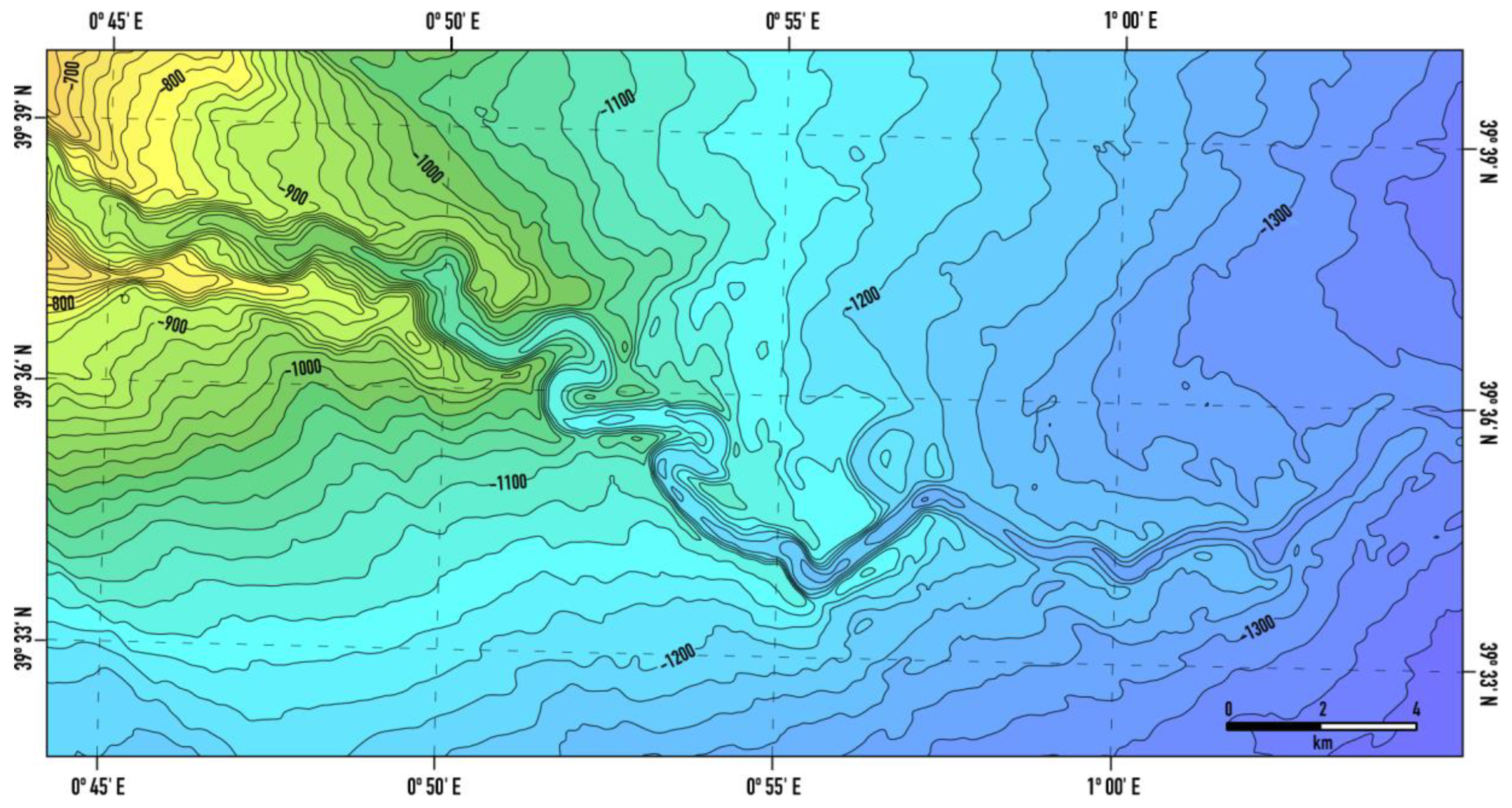
Figure 8.
Shaded relief image of the CGC. The location of some of the morphological elements described in the text is indicated. Two representative topographic profiles mentioned in the text are also shown.
Figure 8.
Shaded relief image of the CGC. The location of some of the morphological elements described in the text is indicated. Two representative topographic profiles mentioned in the text are also shown.
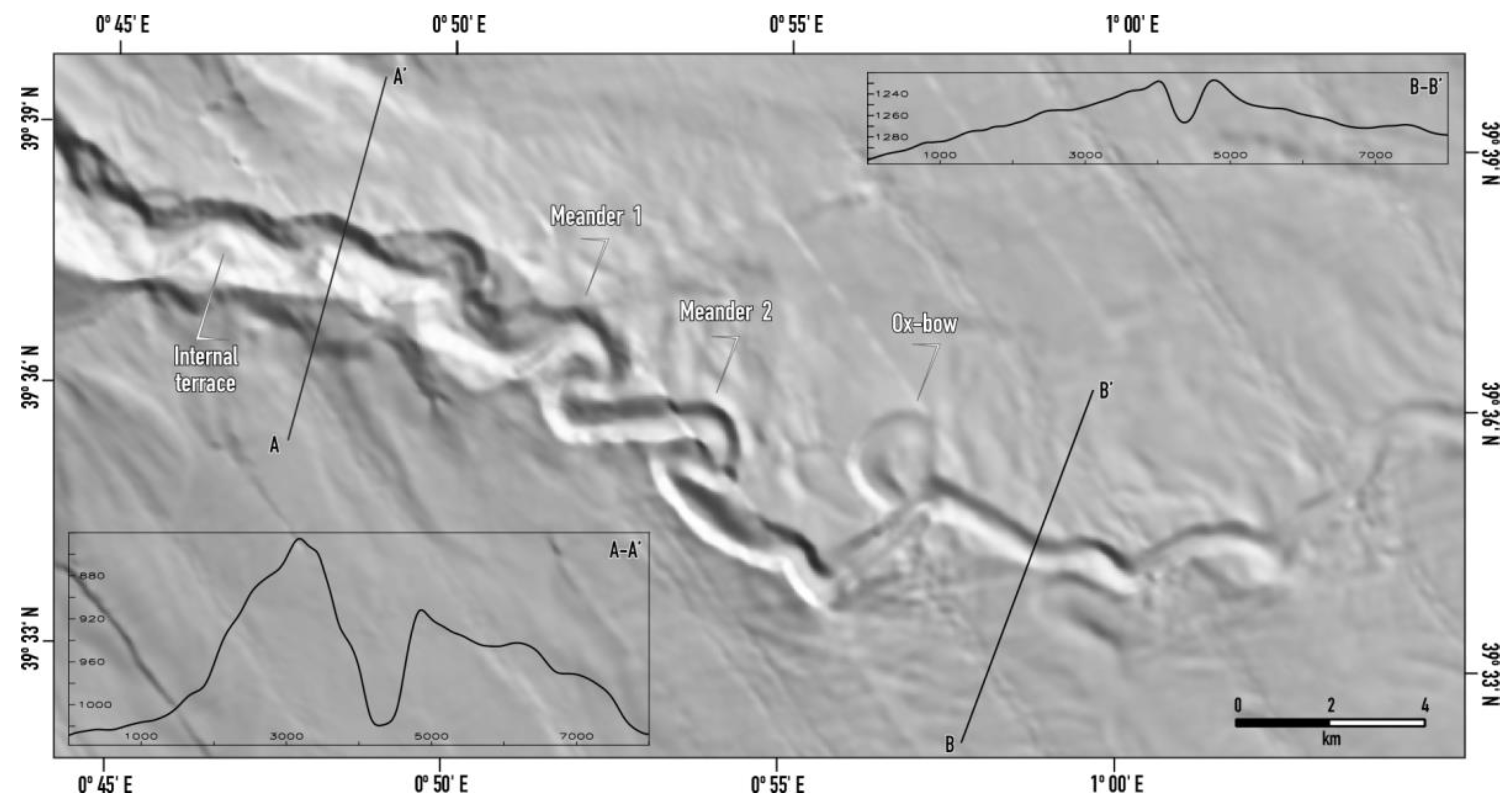
Figure 9.
3D view from the southeast of the CGC. The view is inclined at 28° and vertically exaggerated by x5.
Figure 9.
3D view from the southeast of the CGC. The view is inclined at 28° and vertically exaggerated by x5.
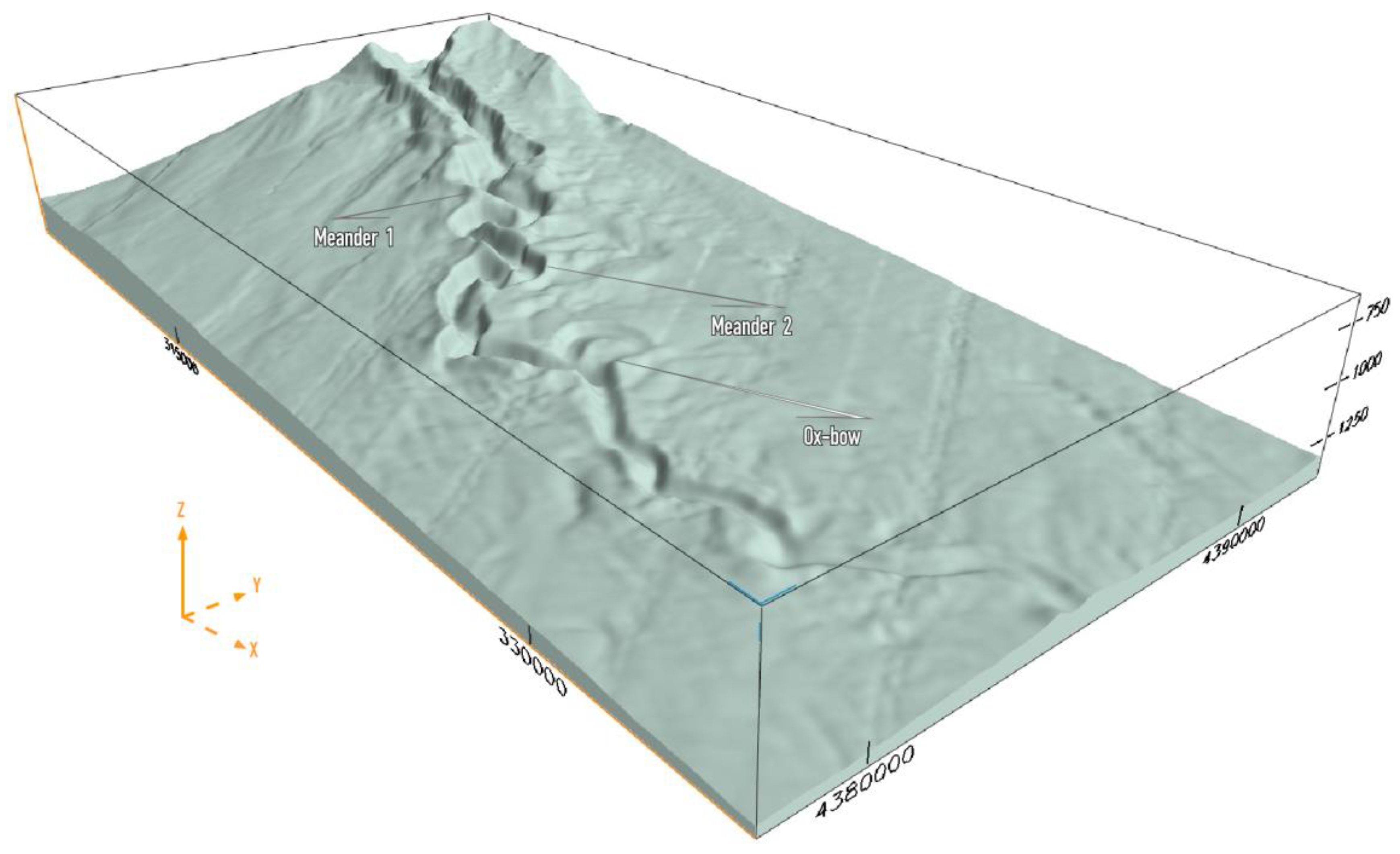
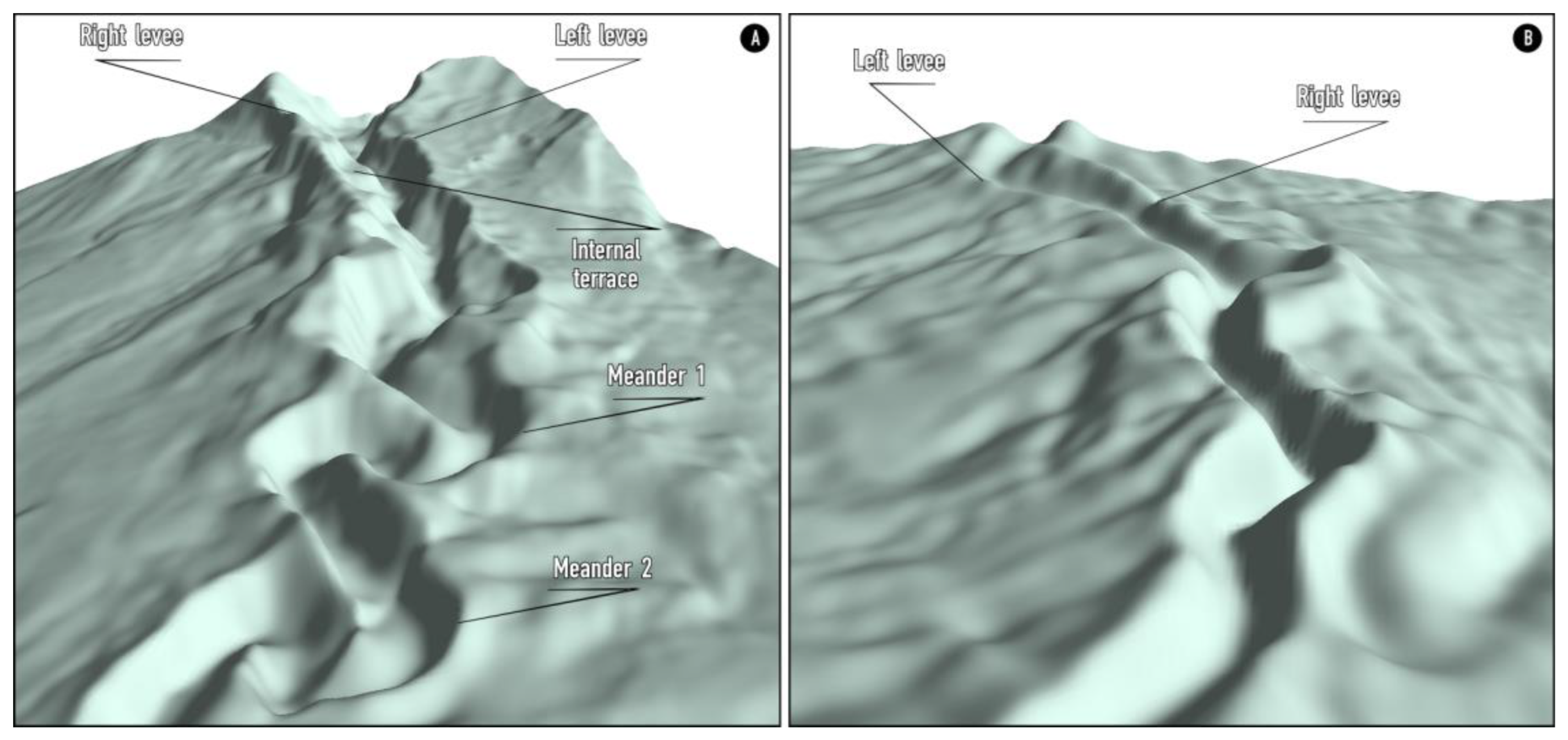
Figure 10.
A: 3D view from the west of the upper CGC course, showing the levees bordering the channel. The view is inclined at 25° and vertically exaggerated by x5. B: 3D view from the east of the lower course of the CGC, showing more symmetrical levees with decreased height. The view is inclined at 40° and vertically exaggerated by x10.
Meander 1 has a radius of 650 m while the radius of meander 2 is 550 m. According to [19], in this type of channel the radius of the meanders tends to decrease with depth. Regardless of the geological context in which it is located, a meander constitutes a form of balance between the slope, the flow, the sedimentary load and the resistance of the channel to erosion. In a TC, turbidity currents circulate episodically, causing erosion. Meanders exaggerate over time, leading to the abandonment of the most accentuated curves. An abandoned meander (ox-bow), like the one downstream show in Figure 8 and Figure 9, has a depth of about 1,200 m, a radius of 600 m, and hangs 45 m above the current channel.
The channel becomes shallower and narrower (Figure 8 and Figure 10B) in the lower course (1200-1300 m), changing to W-E orientation until it disappears into the continental glacis. No distributary channels are observed, or they would be of little relief. The longitudinal morphological variability of the channel is well reflected in the representative topographic profiles of Figure 8. The channel’s relief decreases downward, from a transverse V-profile in the upper sections to a U-profile until termination. These profiles show the elevation (tens of meters) of the levees of the flanks of the channel with respect to the surrounding seabed. The levees can be easily traced and show a marked asymmetry along the channel. The right/southern levee is generally higher than the left/northern levee. This is due to the combined effect of the Coriolis force [51,52], which deflects flows to the right in the northern hemisphere, and the general circulation to the southwest. The existence of such circulation between the Gulf of Lion and the Ibiza Channel has been proven to be at least a thousand meters deep. The intervention of centrifugal force in the meandering sections of the channel is not ruled out either [6,53].
It is thus a channel-levee system whose channel is in a relatively higher position than the seafloor beyond the system, a circumstance that is clearly seen in the maps and 3-D images in Figure 10, Figure 11, Figure 12, Figure 13, Figure 14, Figures 15 and 16. These characteristics would already indicate, according to [7], that the channel would be of depositional type.
The shaded relief image and topograhic profile A-A' in Figure 8 show the marked incision of the channel axis at some point of the CGC. The incision process has led, locally, to the formation of minor courses and hanging internal terraces, a fact that proves the erosive capacity of the turbidity currents that have circulated through the channel. The presence of a course less than 300 m wide embedded in the major course, as well as sand waves and small semicircular scars, especially on the inner left side of the channel, as been indicated by [54] from side-scan sonar images. These scars, cited in other turbidite channels [6,55], would be the result of small landslides in the inner slopes of the channels [56]. The terraces located between the major and minor courses, also identified in other meandering TCs, would be formed in a similar way to fluvial terraces [53]. Gully erosion have also been observed in the internal walls of the main course of the channel. All these morphological evidences confirm the erosive-depositional character of the upper and middle courses of the channel.
4.2. Quantitative Channel Analysis
The quantitative analysis was conducted from 60 control sections distributed across the CGC. These sections were created according to the requirements described in [43]. Additional cross-sections were interpolated between these control sections, approximately 100 m apart, resulting in 423 sections covering all the channel (Figure A1 and Figure A2). The parameters described above have been obtained from each of the interpolated sections.
4.2.1. Planform Geometry
Figure 11 and Table 1 show the plan values for the entire channel. The channel plan parameters were also calculated for intervals or reaches of 50 cross-sections. The number of sections in each reach is arbitrary. While more or fewer sections can affect the results [7], 50 was chosen as the most convenient value, as significant morphological changes occur around multiples of 50 sections.
- Area and length
The total area of the channel is 50 km2 while its axial length is almost 45 km (Table 1 and Figure 11). The length of the valley is slightly over 30 km.
- Slope
The average axial slope is 0.6°, while the average valley slope is 0.87°. By reaches or intervals of 50 sections, it can be observed that the trends of both slopes have an appreciable parallelism except in the final section of the channel where they diverge (Figure 12A). Both slopes decrease, in general terms, with depth, although the axial slope decreases more gently for the same reason. The largest axial gradient is in the first reaches of the channel and gradually decreases, with some local upturn (reach 5). From reach 6 onwards, the axial slope is very low, between 0.28° and 0.36° (4.9 to 6.3 m/km, respectively) (Figure 11 and Figure 12A).
- Sinuosity
The sinuosity index of the channel is 1.46. Following the classification of [57] (low: <1.1; moderate: 1.1-1.5; high: >1.5), the sinuosity is on the border between moderate and high. However, the sinuosity varies along the channel. The subdivision into intervals of 50 sections (Figures 11) shows that the SI increases appreciably from kilometre 11, where the pronounced meanders begin. The fourth and fifth reaches have sinuosity indices close to 2 (Table 1 and Figure 12A). After these reaches, the SI decreases to 1.1 in the lowest course of the channel.
- Slope-sinuosity relationship
The slope and sinuosity parameters are closely linked, and the sinuosity of the TCs is affected by slope variations [7,19]. The adjusted sinuosity/slope index curve of the channel (Figure 12B) resembles those obtained in laboratory tests by [58]. It is also consistent with the curves obtained by [20] for several submarine channels. The shape of the adjusted curve is explained by the fact that as the slope increases, so does the sinuosity of the channel, thus maintaining an optimal slope that favours the accommodation of turbidity currents and the evacuation of the corresponding sedimentary load. This situation is maintained until a threshold slope is reached from which the channel seeks a more direct route downstream, resulting in a decrease in sinuosity.
4.2.2. Cross-Sectional Geometry
Table 2 shows the maximum, minimum, and average values for each cross-sectional parameter considered. Graphics illustrating the relationships between different cross-sectional parameters are shown in Figure 13. In all graphics, the lower axis of abscissas corresponds to the sequential numbering of the sections from the beginning of the channel to its end. The upper axis of abscissas indicates the distance of the sections along the axis of the channel.
- Depth of axis channel and levees
The axial depth of the channel ranges from 865 m to 1325 m (Table 2 and Figure 13A). The resulting profile is slightly concave and quite smooth. The depths of the crests of the levees in the studied channel are between 663 m and 1311 m. The depth profiles of the crests of the levees are similar to the axial profile, although they present more and greater irregularities. Since the height of the flanks of the channel decreases downslope, the profiles of the crest of the levees approach the axial profile in the same direction. The practical superposition of the depth profiles of the crest of the levees along the lower course reveals that it is in this lower part where the levees are more symmetrical.
- Channel height
The average channel flank height is 95 m, with a maximum of 202 m on the left flank and a minimum of 10.4 m on the right flank (Table 2). The average height profile of the channel flanks is divided into three segments (Figure 13B). The segment A, 15 km long, reaches section 150, in the middle of meander 1 (Figure 8 and Figure 9), with a total descent of 150 m (from 200 to 50 m) in the height of the flanks of the channel. This descent is particularly steep in the last 5 km of the segment. With a gradient of loss of flank height of 1 m every 100 m. The segment B, 19 km long, is marked by an initial ascent of flank height, followed by several marked oscillations, and a steep drop shortly before section 300 (Figure 13B). In this second segment, the average height of the flanks of the channel is 75 m. After a short initial ascent, in the third and final segment C, the average height of flanks descends progressively, although not without ups and downs, being clearly below 50 m. The average height of the channel flanks is only 13 m in the lowest course. In this segment, the gradient of height loss is 1 m every 400 m.
- Height difference between flanks
The graphic of this parameter shows that the right flank is higher (positive values in Figure 13C) than the left along almost the entire CGC, especially in the straighter sections. This is due to the Coriolis force [52,59]. Negative values are concentrated in the channel’s meanders and curves, where centrifugal force is predominant.
- Width
Channel widths range from 3370 m to 660 m, with an average width of 1325 m. The greatest widths are in the upper course of the channel. The main variations in width are reflected by prominent ridges in the graphic of Figure 13D. The main decrease in width occurs between sections 100 and 140, coinciding with the beginning of the first marked meander and, practically, with the lower course of segment A (Figure 13B). Downstream, the channel width presents minor oscillations, averaging 1,000 m.
- Section area
The average value of the area of the section is 58500 m2, with a maximum value of 379000 m2 at the beginning of the channel and a minimum of 3455 m2 in one of the cross-sections of the lower course. Figure 13E shows the section area variations, similar to flank height and channel width profiles but smoother. Segments A, B, and C identified in Figure 13B can also be differentiated with a slight lag.
- Width-to-height ratio
The average value of this parameter for the entire channel is 18. It is interesting to note that in the graph in Figure 13F the width-height relationship remains within a narrow range of variation (10-20) for segments A and B, with only two peaks exceeding the value 20, corresponding to the central part of meanders 1 and 2 (Figure 8). In segment C, the ratio increases with ups and downs, reaching over 50 in the most distal sections. The relatively high values obtained are typical of modern turbidite channels [60,61].
4.3. 3D Visualization and Channel Volume
The 3D visualization of the potential sediment fill of the CGC is illustrated in Figure 14. The calculated volume (2.2 km3) of this geobody corresponds to the capacity of the channel in accordance with the considerations set out above. Consequently, neither the nature of the filling material nor its porosity has been taken into account. However, in this type of channel, the infill is usually dominated by fine-grained sizes, with varying proportions of sands [62]. The volume obtained corresponds to the modern geometry of the channel and, therefore, the hypothetical presence of materials that could have begun to fill it has not been considered either.
4.4. Morphosedimentary Interpretation
The studied channel, though small, exhibits morphological features similar to other turbidite channels fed by extensive river basins and dominated by mud inputs [4,63]. The high sinuosity index of some of its reaches and its relatively low slopes would lead to classify it mainly as a depositional type channel [7]. Flank heights, usually less than 150 m, and well-developed levees are also characteristic of depositional channels [20,22].
The analysis of some of the geometric parameters of the CGC allows estimating the characteristics of the density flows responsible for their formation, maintenance, and modification. Sinuosity index close to 2 and gentle slopes such as those observed (Figure 12B) would be typical of systems fed by turbidity currents that mainly transport fine-grained materials that are easy to resuspend [64]. The thickness of the turbidity currents that have circulated through the channel must have been, at least, somewhat greater than the height of its flanks, a circumstance that would have made possible the accumulation by overflow of the sediments that form the levees and wings of the channel-levee system.
The general trend towards a decrease in the height of the channel flanks in a downward direction is in line with the decrease in the size of the channel in the same direction. This decrease would be a consequence of the progressive loss of energy and much of the material transported by the turbidity currents as they advance within the channel. According to [1], as a result of the gradual loss of its finer components, the turbidity currents would become thinner and more concentrated towards the final reaches of the channel, where the slopes are lower. However, the presence of levees, although less developed, in the lower course of our CGC indicates that at least part of the fine-grained sedimentary load reaches the end of it.
On the other hand, the concave and relatively smooth shape of the depth profile of the CGC axis (Figure 13A) suggests that an equilibrium profile has been practically achieved [50]. The generation of meanders has undoubtedly contributed to the development of this equilibrium profile. The existence of such a situation of equilibrium in a longitudinal direction would imply that the profile of the channel would also be in equilibrium [26]. However, the abandoned and hanging ox-bow (Figure 8 and Figure 9) and local evidence of erosion would indicate episodes of rupture of the equilibrium profile in the recent past.
This channel, like the rest of the TCs of the ECM, has a relatively ephemeral life geologically speaking, since the same processes responsible for its formation generate new channels and leave the old ones abandoned as a result of episodes of avulsion and excavation of the thalweg, as evidenced by numerous evidences [31]. The increasing embedding of the active channel tends to leave abandoned sections hanging, as can be seen in the case of the strangled and hanging ox-bow in Figure 8 and Figure 9. The abandoned sections are progressively disfigured by internal and external landslides, filling with the contribution of hemipelagic materials, and phagocytosis by younger channels. The channel would be active episodically and the turbidity currents that circulate inside are responsible for rejuvenating it morphologically and keeping it open as a preferred route for transporting sediments to the deep basin.
5. Conclusions
The results of this work contribute to the quantitative characterization and 3D modelling of turbidite channels. The methodology accurately describes the morphology of the Columbretes Grande channel, located on the Ebro continental margin, and calculates its geometric parameters. Furthermore, the extraction and 3D visualization of the channel geobody is realistic and allows precise volumetric calculations. The morphosedimentary interpretation of the channel, whose concave and smooth profile, high sinuosity of some of its reaches, and relatively low slopes, the presence of levees, and the height of its flanks, allow it to be classified as depositional type.
In addition to the quantitative aspects analysed, the resolution and quality of the 3D visualizations also contribute to improving the interpretation and understanding of the processes that generate and modify this type of channels. All this provides a precise answer to the need expressed by several authors to use the geometric parameters of the channels for a more quantitative and objective classification of the sedimentary systems that these morphologies feed [7,19,20,61].
Precisely, many of these sedimentary deposits are in fact the main hydrocarbon reservoirs in the world. As it will be increasingly necessary to go into deep environments to find new reserves [17,65], 3D morphometric analysis, both of fossil turbidite channels but also of their modern analogues, will be more and more important to develop predictive models that allow planning the exploration and exploitation of those reservoirs [48,62,66].
Funding
This research was funded by the research project “"Estudio oceanográfico multidisciplinar del Mar Catalano-Balear" (reference: AMB94-0706-C02), funded by the Spanish “Comisión Interministerial de Ciencia y Tecnología (CICYT)”, the research project “EUROMARGE-NB” (reference: MAS2-CT93-0053), funded by European Union, and the research project “Mass Transfer and Ecosystems Response” (reference: MAS·-CT96-0051), funded by European Union.
Data Availability Statement
The data of this study are available upon request to the author.
Acknowledgments
The author acknowledges the financial support from the Catalan Government to the “Grup de Recerca Consolidat en Geociències Marines” (grant no. 2021 SGR 01195).
Conflicts of Interest
The author declares no conflicts of interest.
Abbreviations
The following abbreviations, listed in alphabetical order, are used in the main text of the manuscript:
| AHF | Average Height of Flanks |
| CA | Channel Area |
| CCS | Canyon-Channel System |
| CGC | Columbretes Grande Channel |
| CL | Channel Length |
| CLS | Channel-Levee System |
| CS | Channel Slope |
| CSA | Channel Section Area |
| CSW | Channel Section Width |
| DCA | Depth of the Channel Axis |
| DLL | Depth of the crest of the Left Levee |
| DRL | Depth of the crest of the Right Levee |
| ECM | Ebro Continental Margin |
| HDF | Height Difference between Flanks |
| HLF | Height of the Left Flank |
| HRF | Height of the Right Flank |
| ISN | Interpolated Section Number |
| SDC | Section Distance since the beginning of the Channel |
| SI | Sinuosity Index |
| TC | Turbidite Channel |
| VL | Valley Length |
| VS | Valley Slope |
| WHR | Width to Height Ratio of the section |
Appendix A
Figure A1.
Distribution of control sections (in orange) and interpolated sections (in black). The interpolated cross-section number is indicated in intervals of 10 sections.
Figure A1.
Distribution of control sections (in orange) and interpolated sections (in black). The interpolated cross-section number is indicated in intervals of 10 sections.
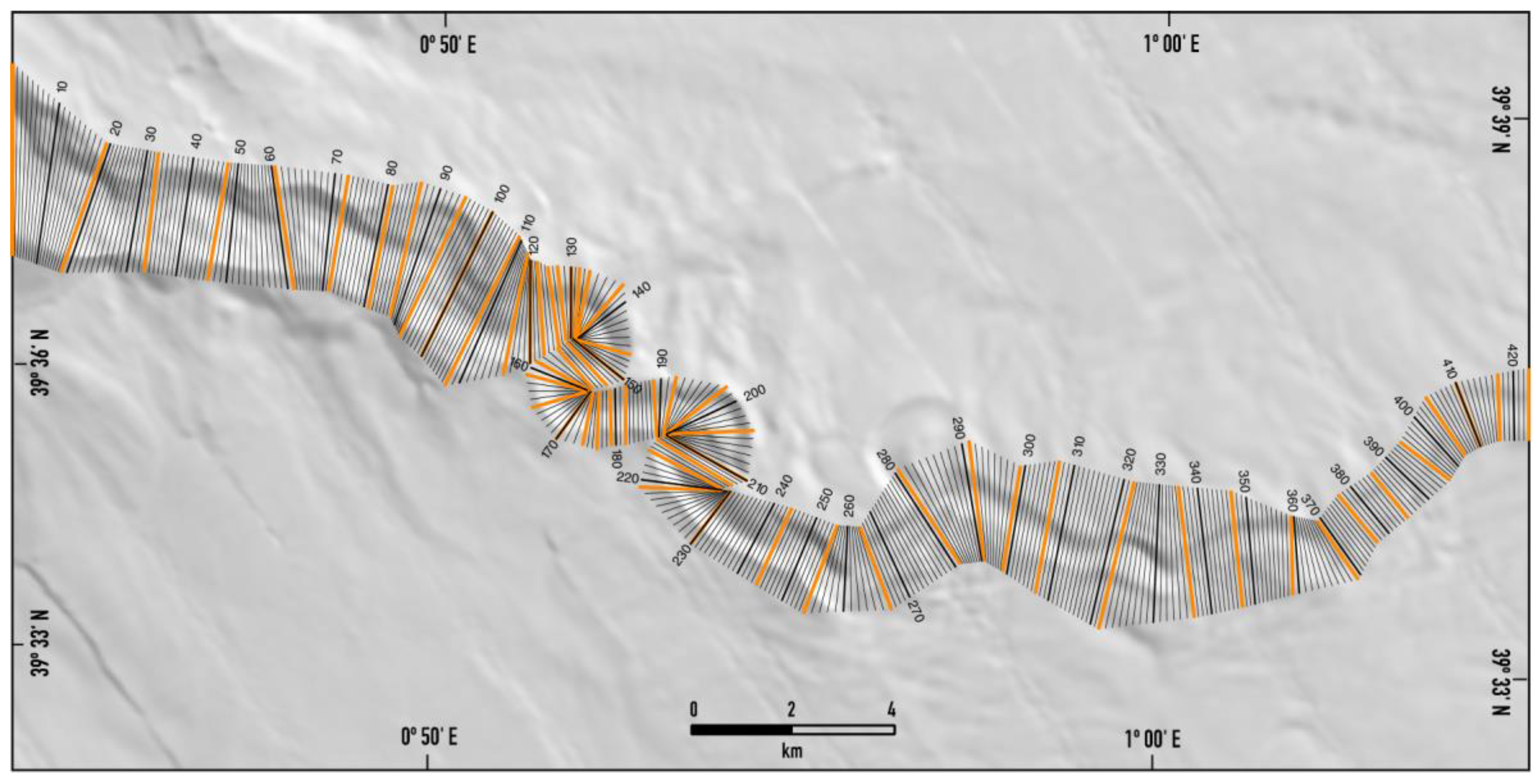
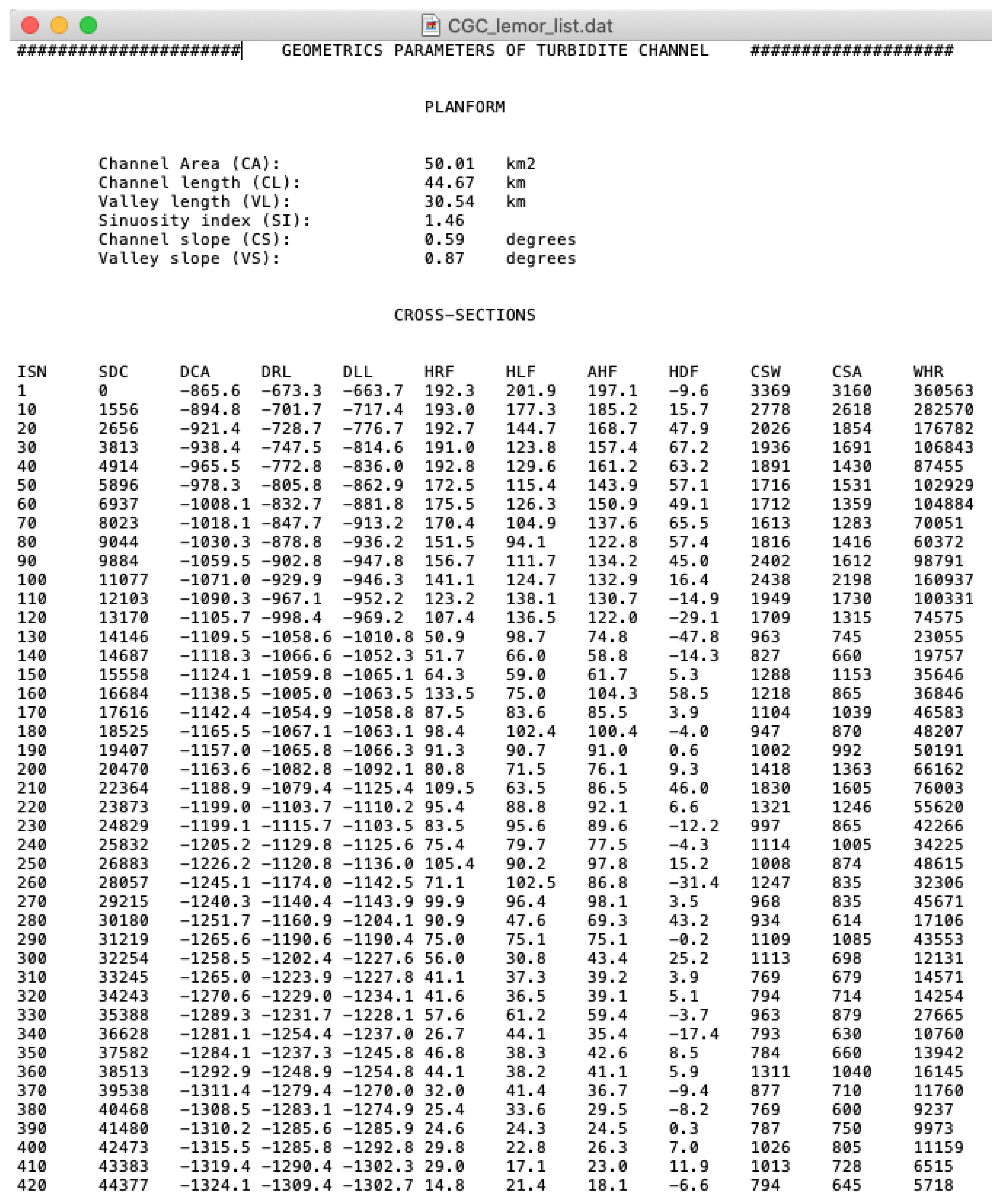
Figure A2.
Output ASCII file with values resulting from Lemor's calculations. The interpolated cross-section number is indicated in intervals of 10 sections. DCA: Depth of the channel axis; DRL: Depth of the crest of the right levee; DLL: Depth of the crest of the left levee; HRF: Height of the right flank; HLF: Height of the left flank; AHF: Average height of flanks; HDF: Height difference between flanks ; CSW: Channel section width; CSA: Channel section area; WHR: Width to height ratio of the section.
References
- Babonneau, N.; Savoye, B.; Cremer, M.; Klein, B. Morphology and Architecture of the Present Canyon and Channel System of the Zaire Deep-Sea Fan. Marine and Petroleum Geology 2002, 19, 445–467. [CrossRef]
- Canals, M.; Casamor, J.L.; Lastras, G.; Monaco, A.; Acosta, J.; Berné, S.; Loubrieu, B.; Weaver, P.P.E.; Grehan, A.; Dennielou, B. The Role of Canyons in Strata Formation. Oceanography 2004, 17. [CrossRef]
- Hasenhündl, M.; Talling, P.J.; Pope, E.L.; Baker, M.L.; Heijnen, M.S.; Ruffell, S.C.; Da Silva Jacinto, R.; Gaillot, A.; Hage, S.; Simmons, S.M.; et al. Morphometric Fingerprints and Downslope Evolution in Bathymetric Surveys: Insights into Morphodynamics of the Congo Canyon-Channel. Front. Earth Sci. 2024, 12. [CrossRef]
- Skene, K.I.; Piper, D.J.W.; Hill, P.S. Quantitative Analysis of Variations in Depositional Sequence Thickness from Submarine Channel Levees. Sedimentology 2002, 49, 1411–1430. [CrossRef]
- Fildani, A. Submarine Canyons: A Brief Review Looking Forward. Geology 2017, 45, 383–384. [CrossRef]
- McHugh, C.M.G.; Ryan, W.B.F. Sedimentary Features Associated with Channel Overbank Flow: Examples from the Monterey Fan. Marine Geology 2000, 163, 199–215.
- Clark, J.D.; Pickering, K.T. Submarine Channels: Processes and Architecture; Vallis Press: London, 1996;
- Wonham, J.P.; Jayr, S.; Mougamba, R.; Chuilon, P. 3D Sedimentary Evolution of a Canyon Fill (Lower Miocene-Age) from the Mandorove Formation, Offshore Gabon. Marine and Petroleum Geology 2000, 17, 175–197.
- Peakall, J.; McCaffrey, B.; Kneller, B. A Process Model for the Evolution, Morphology, and Architecture of Sinuous Submarine Channels. Journal of Sedimentary Research 2000, 70, 434–448.
- Damuth, J.E.; Kowsmann, R.O.; Flood, R.D.; Belderson, R.H.; Gorini, M.A. Age Relationships of Distributary Channels on Amazon Deep-Sea Fan: Implications for Fan Growth Pattern. Geology 1983, 11, 470–473.
- Deptuck, M.E.; Sylvester, Z. Submarine Fans and Their Channels, Levees, and Lobes. In Submarine Geomorphology; Micallef, A., Krastel, S., Savini, A., Eds.; Springer International Publishing: Cham, 2018; pp. 273–299 ISBN 978-3-319-57852-1.
- Flood, R.D.; Manley, P.L.; Kowsmann, R.O.; Appi, C.J.; Pirmez, C. Seismic Facies and Late Quaternary Growth of Amazon Submarine Fan. In Seismic Facies and Sedimentary Processes of Submarine Fans and Turbidite Systems; En, P.W., Link, M.H., Eds.; Springer: New York, 1991; pp. 415–434.
- Canals, M.; Alonso, B.; Ercilla, G.; Farrán, M.; Sorribas, J.; Baraza, J.; Calafat, A.M.; Casamor, J.L.; Estrada, F.; Masson, D.; et al. Dinámica de los canales submarinos del talud y el glacis continentales del Ebro (Mediterráneo-noroccidental) a partir de imágenes acústicas de alta resolución. Geogaceta 1996, 20, 363–367.
- Alonso, B.; Ercilla, G. Introducción: sistemas turbidíticos y canales medio-oceánicos. In Valles Submarinos y Sistemas Turbidíticos Modernos; En, B.A., Ercilla, G., Eds.; CSIC: Barcelona, 2000; pp. 19–66.
- Shanmugam, G.; Moiola, R.J. Submarine Fans: Characteristics, Models, Classification, and Reservoir Potential. Earth-Science Reviews 1988, 24, 383–428.
- Nibbelink, K. Modeling Deepwater Reservoir Analogs through Analysis of Recent Sediments Using Coherence, Seismic Amplitude, and Bathymetry Data, Sigsbee Escarpment, Green Canyon, Gulf of Mexico. The Leading Edge 1999, 18, 550–561.
- Weimer, P.; Slatt, R.M. Turbidite Systems; Part I, Sequence and Seismic Stratigraphy. The Leading Edge 1999, 18, 454–463.
- Fonnesu, F. 3D Seismic Images of a Low-Sinuosity Slope Channel and Related Depositional Lobe (West Africa Deep-Offshore). Marine and Petroleum Geology 2003, 20, 615–629. [CrossRef]
- Flood, R.D.; Damuth, J.E. Quantitative Characteristics of Sinuous Distriburary Channels on the Amazon Deep-Sea Fan. GSA Bulletin 1987, 98, 728–738.
- Clark, J.D.; Kenyon, N.H.; Pickering, K.T. Quantitative Analysis of the Geometry of Submarine Channels: Implications for the Classification of Submarine Fans. Geology 1992, 20, 633–636.
- Klaucke, I.; Hesse, R.; Ryan, W.B.F. Flow Parameters of Turbidity Currents in a Low-Sinuosity Giant Deep-Sea Channel. Sedimentology 1997, 44, 1102–1997.
- Morris, W.R.; Normark, W.R. Sedimentologic and Geometric Criteria for Comparing Modern and Ancient Sandy Turbidite Elements. Deep-Water Reservoirs of the World. In Proceedings of the GCSSEPM Foundation 20th Annual Research Conference; Estados Unidos: Houston, Texas, 2000; Vol. December 3-6, pp. 606–623.
- Stow, D.A.V.; Mayall, M. Deep-Water Sedimentary Systems: New Models for the 21st Century. Marine and Petroleum Geology 2000, 17, 125–135.
- Clark, J.D.; Gardiner, A.R. Outcrop Analogues for Deep-Water Channel and Levee Genetic Units from the Grès d’Annot Turbidite System. Deep-Water Reservoirs of the World. In Proceedings of the GCSSEPM Foundation 20th Annual Research Conference; Estados Unidos: Houston, Texas, 2000; pp. 175–189.
- Wen, R. 3D Modeling of Stratigraphic Heterogeneity in Channelized Reservoirs, Methods and Applications in Seismic Attributes Facies Classification. Canadian Society of Exploration Geophysicists (CSEG) Recorder 2004, 39–45.
- Estrada, F.; Ercilla, G.; Alonso, B. Quantitative Study of a Magdalena Submarine Channel (Caribbean Sea): Implications for Sedimentary Dynamics. Marine and Petroleum Geology 2005, 22, 623–635. [CrossRef]
- Iglesias, O.; Lastras, G.; Canals, M.; Olabarrieta, M.; González, M.; Aniel-Quiroga, Í.; Otero, L.; Durán, R.; Amblas, D.; Casamor, J.L.; et al. The BIG’95 Submarine Landslide-Generated Tsunami: A Numerical Simulation. Journal of Geology 2012, 120. [CrossRef]
- Nelson, C.H. Estimated Post-Messinian Sediment Supply and Sedimentation Rates on the Ebro Continental Margin, Spain. Marine Geology 1990, 95, 395–418.
- Acosta, J.; Canals, M.; López-Martínez, J.; Muñoz, A.; Herranz, P.; Urgeles, R.; Palomo, C.; Casamor, J.L. The Balearic Promontory Geomorphology (Western Mediterranean): Morphostructure and Active Processes. Geomorphology 2003, 49. [CrossRef]
- Alonso, B.; Canals, M.; Palanques, A.; Rehault, J.-P. A Deep-Sea Channel in the Northwestern Mediterranean Sea: Morphology and Seismic Structure of the Valencia Channel and Its Surroundings. Mar Geophys Res 1995, 17, 469–484. [CrossRef]
- Canals, M.; Casamor, J.L.; Urgeles, R.; Lastras, G.; Calafat, A.M.; Batist, M.; Masson, D.; Berné, S.; Alonso, B.; Hughes-Clarke, J.E. The Ebro Continental Margin, Western Mediterranean Sea: Interplay between Canyon-Channel Systems and Mass Wasting Processes. In Proceedings of the Deep-water Reservoirs of the World, GCSSEPM Foundation 20th Annual Research Conference; Estados Unidos: CD edition, Houston, Texas, 2000; pp. 152–174.
- Maillard, A.; Mauffret, A. Structure and Volcanism of the Valencia Trough, North-Western Mediterranean. Bulletin - Societe Geologique de France 1993, 164, 365–383.
- Lastras, G.; Canals, M.; Urgeles, R.; De Batist, M.; Calafat, A.M.; Casamor, J.L. Characterisation of the Recent BIG’95 Debris Flow Deposit on the Ebro Margin, Western Mediterranean Sea, after a Variety of Seismic Reflection Data. Marine Geology 2004, 213. [CrossRef]
- O’Connell, S.; Ryan, W.B.F.; Normark, W.R. Modes of Development of Slope Canyons and Their Relation to Channel and Levee Features on the Ebro Sediment Apron, off-Shore Northeastern Spain. Marine and Petroleum Geology 1987, 4, 308.
- Nelson, C.H.; Maldonado, A. Factors Controlling Depositional Patterns of Ebro Turbidity Systems, Mediterranean Sea. AAPG Bulletin 1988, 72, 698–716.
- Danobeitia, J.J.; Alonso, B.; Maldonado, A. Geological Framework of the Ebro Continental Margin and Surrounding Areas. Marine Geology 1990, 95, 265–287.
- Alonso, B.; Canals, M.; Got, H.; Maldonado, A. Sea Valleys and Related Depositional Systems in the Gulf of Lions and Ebro Continental Margins. AAPG Bulletin 1991, 75, 1195–1213.
- Alonso, B. El sistema turbidítico del Ebro: evolución morfo-sedimentaria durante el Plio-Cuaternario. In Valles Submarinos y Sistemas Turbidíticos Modernos; En, B.A., Ercilla, G., Eds.; CSIC: Barcelona, 2000; pp. 91–112.
- Medialdea, T.; Somoza, L.; Leon, R.; Lobato, A. Mapa Geomorfológico. Mar Balear 2021.
- Amblas, D.; Gerber, T.P.; Canals, M.; Pratson, L.F.; Urgeles, R.; Lastras, G.; Calafat, A.M. Transient Erosion in the Valencia Trough Turbidite Systems, NW Mediterranean Basin. Geomorphology 2011, 130, 173–184. [CrossRef]
- Casamor, J.L. Introducción al 3-D Con El Programa earthVision; Universitat de Barcelona, 2013; p. 14;
- Guglielmo, G.; Jackson, M.; A., P.; Vendeville, B.C. Three-Dimensional Visualization of Salt Walls and Associated Fault Systems. AAPG Bulletin 1997, 81, 46–61.
- Casamor, J.L. Modelización y Visualización 3-D En Geociencias Marinas. PhD Thesis, Universitat de Barcelona, 2006.
- Nordfjord, S.; Goff, J.A.; Austin, J.; A., J.; Sommerfield, C.K. Seismic Geomorphology of Buried Channel Systems on the New Jersey Outer Shelf: Assessing Past Environmental Conditions. Marine Geology 2005, 214, 339–364.
- Gibling, M.R. Width and Thickness of Fluvial Channel Bodies and Valley Fills in the Geological Record: A Literature Compilation and Classification. Journal of Sedimentary Research 2006, 76, 731–770. [CrossRef]
- Straub, K.M.; Mohrig, D. Quantifying the Morphology and Growth of Levees in Aggrading Submarine Channels. J. Geophys. Res. 2008, 113, 2007JF000896. [CrossRef]
- Balic, N.; Koch, B. Canscan - an Algorithm for Automatic Extraction of Canyons. Remote Sensing 2009, 1, 197–209. [CrossRef]
- McHargue, T.; Pyrcz, M.J.; Sullivan, M.D.; Clark, J.D.; Fildani, A.; Romans, B.W.; Covault, J.A.; Levy, M.; Posamentier, H.W.; Drinkwater, N.J. Architecture of Turbidite Channel Systems on the Continental Slope: Patterns and Predictions. Marine and Petroleum Geology 2011, 28, 728–743. [CrossRef]
- Cerrillo-Escoriza, J.; Lobo, F.J.; Puga-Bernabéu; Bárcenas, P.; Mendes, I.; Pérez-Asensio, J.N.; Durán, R.; Andersen, T.J.; Carrión-Torrente; García, M.; et al. Variable Downcanyon Morphology Controlling the Recent Activity of Shelf-Incised Submarine Canyons (Alboran Sea, Western Mediterranean). Geomorphology 2024, 453. [CrossRef]
- Pirmez, C.; Imran, J. Reconstruction of Turbidity Currents in Amazon Channel. Marine and Petroleum Geology 2003, 20, 823–849.
- Cossu, R.; Wells, M.G. The Evolution of Submarine Channels under the Influence of Coriolis Forces: Experimental Observations of Flow Structures. Terra Nova 2013, 25, 65–71. [CrossRef]
- Allen, C.; Peakall, J.; Hodgson, D.M.; Bradbury, W.; Booth, A.D. Latitudinal Changes in Submarine Channel-Levee System Evolution, Architecture and Flow Processes. Front. Earth Sci. 2022, 10, 976852. [CrossRef]
- Nakajima, T.; Satoh, M.; Okamura, Y. Channel-Levee Complexes, Terminal Deep-Sea Fan and Sediment Wave Fields Associated with the Toyama Deep-Sea Channel System in the Japan Sea. Marine Geology 1998, 147, 25–41. [CrossRef]
- Canals, M.; Alonso, B.; Ercilla, G.; Farrán, M.; Sorribas, J.; Baraza, J.; Calafat, A.M.; Casamor, J.L.; Estrada, F.; Masson, D.; et al. Dinámica de los canales submarinos del talud y el glacis continentales del Ebro (Mediterráneo-noroccidental) a partir de imágenes acústicas de alta resolución. Geogaceta 1996, 20, 363–367.
- Lewis, K.B.; Pantin, H.M. Channel-Axis, Overbank and Drift Sediment Waves in the Southern Hikurangi Trough, New Zealand. Marine Geology 2002, 192, 123–151. [CrossRef]
- Posamentier, H.W. Depositional Elements Associated with a Basin Floor Channel-Levee System: Case Study from the Gulf of Mexico. Marine and Petroleum Geology 2003, 20, 677–690. [CrossRef]
- Schumm, S.A. Sinuosity of Alluvial Rivers on the Great Plains. GSA Bulletin 1963, 74, 1089–1099.
- Schumm, S.A.; Khan, H.R. Experimental Study of Channel Patterns. GSA Bulletin 1972, 83, 1755–1770.
- Sylvester, Z.; Pirmez, C. Latitudinal Changes in the Morphology of Submarine Channels: Reevaluating the Evidence for the Influence of the Coriolis Force. In Latitudinal Controls on Stratigraphic Models and Sedimentary Concepts; Fraticelli, C.M., Ed.; SEPM (Society for Sedimentary Geology), 2019; pp. 82–92 ISBN 978-1-56576-346-3.
- Clark, J.D.; Pickering, K.T. Architectural Elements of Submarine Channels, Growth Patterns and Application to Hydrocarbon Exploration. AAPG Bulletin 1996, 80, 194–221.
- Pettinga, L.; Jobe, Z.; Shumaker, L.; Howes, N. Morphometric Scaling Relationships in Submarine Channel–Lobe Systems. Geology 2018, 46, 819–822. [CrossRef]
- Slatt, R.M.; Weimer, P. Turbidite Systems; Part 2, Subseismic-Scale Reservoir Characteristics. The Leading Edge 1999, 18, 562–567.
- Pirmez, C.; Beaubouef, R.T.; Friedmann, S.J.; Mohrig, D.C. Equilibrium Profile and Baselevel in Submarine Channels: Examples from Late Pleistocene Systems and Implications for the Architecture of Deepwater Reservoirs. In Proceedings of the Deep-water Reservoirs of the World, GCSSEPM Foundation 20th Annual Research Conference; Estados Unidos: Houston, Texas, 2000; pp. 782–804.
- Schumm, S.A. Evolution and Response of the Fluvial System: Sedimentologic Implications. Soc. Econ. Paleon. Mineral. Spec. Pub 1981, 31, 19–29.
- Mayall, M.; Jones, E.; Casey, M. Turbidite Channel Reservoirs—Key Elements in Facies Prediction and Effective Development. Marine and Petroleum Geology 2006, 23, 821–841. [CrossRef]
- Bryant, I.; Carr, D.; Cirilli, P.; Drinkwater, N.; McCormick, D.; Tilke, P.; Thurmond, J. Use of 3D Digital Analogues as Templates in Reservoir Modelling. Petroleum Geoscience 2000, 6, 195–201.
Figure 1.
Colour-shaded relief map of the southern Catalan-Balearic basin, showing main structural elements and locations of important CCSs in the ECM. The black box corresponds to Figure 2. To avoid further confusion, because over the years the main CCSs have been assigned different names by various author, here is used the general nomenclature of [39]. CCS-CG: Columbretes Grande CCS; CCS-CC: Columbretes Chico CCS; CCS-HI: Hirta CCS; CCS-TB: Torreblanca CCS; CCS-VI: Vinaroz CCS; CCS-TO: Tortosa CCS; SM-B: Bertán Seamount; SM-C: Cresques Seamount; SM-B: Bertrán Seamount; SM-D: Sa Dragonera Seamount; SM-B: Soller Seamount.
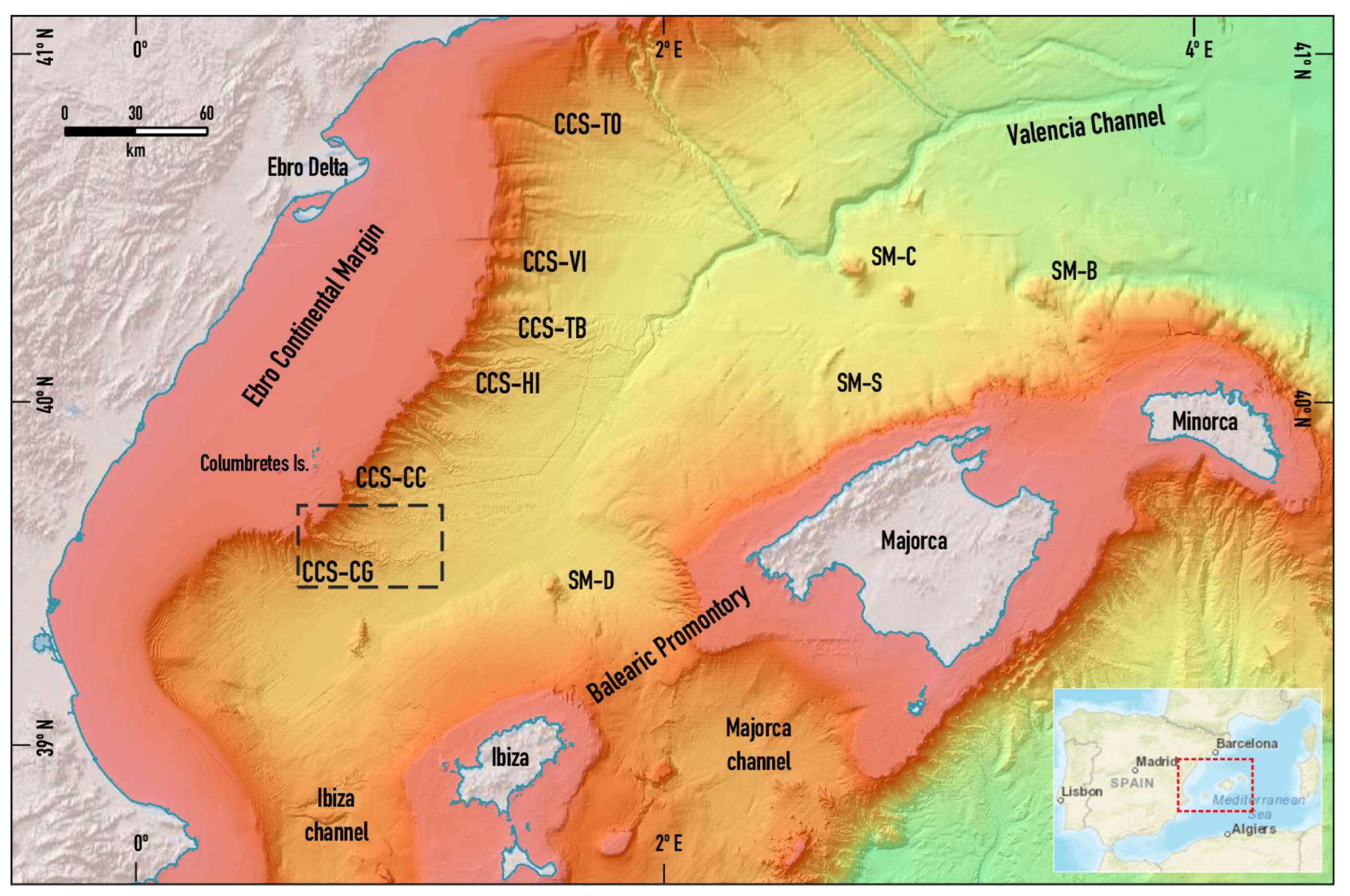
Figure 2.
General bathymetric map of the CCS of Columbretes Grande. See its position within the ECM in Figure 1. The red box corresponds to channel shown in Figure 7. Isobaths are equidistant at 50 m.
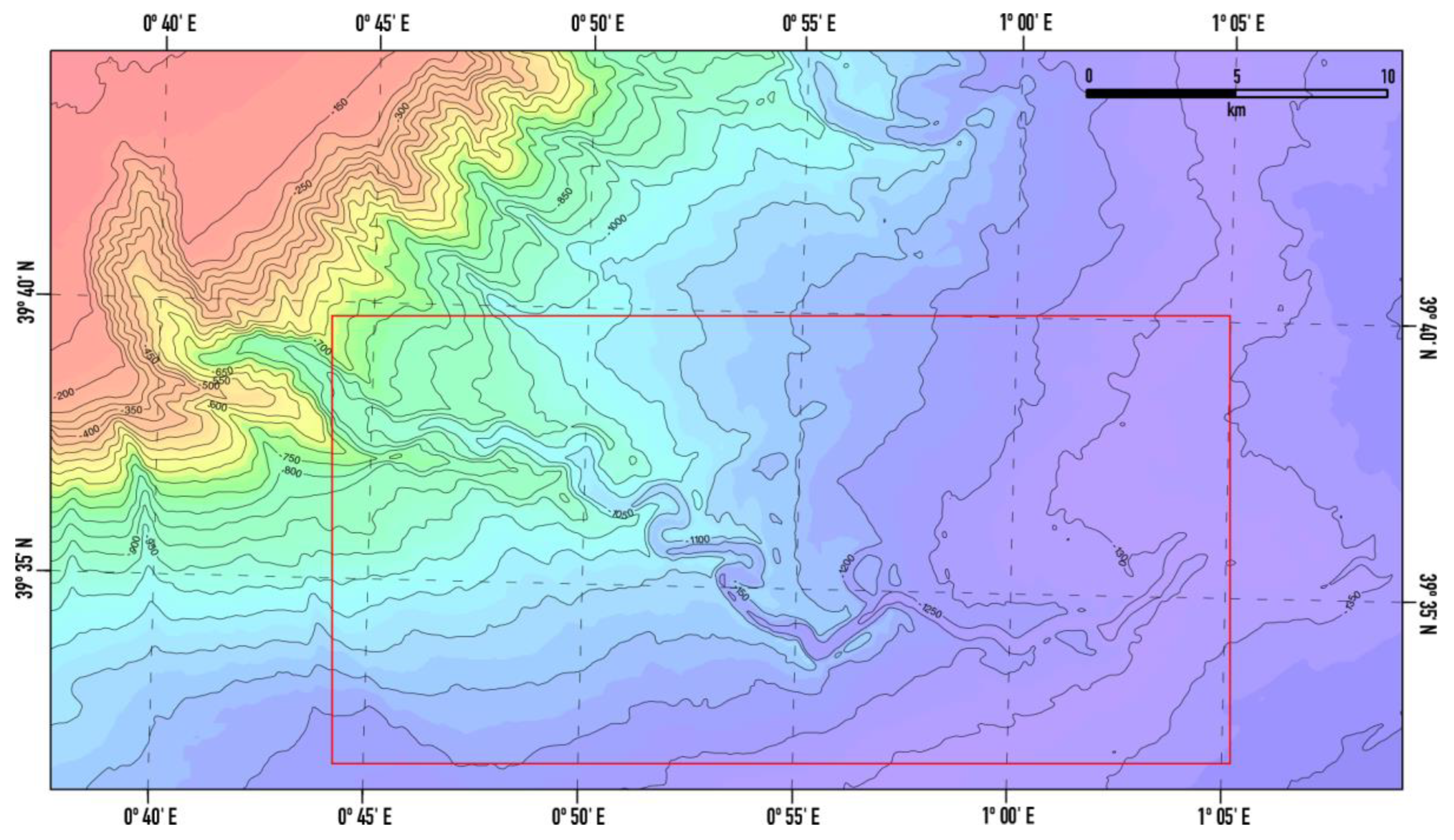
Figure 3.
Flowchart of the methodology used (modified from [43]). All representations, including those of the scripts results, have been created with earthVision using a small sector of the 2D bathymetric grid of the upper course of the CGC.
Figure 3.
Flowchart of the methodology used (modified from [43]). All representations, including those of the scripts results, have been created with earthVision using a small sector of the 2D bathymetric grid of the upper course of the CGC.
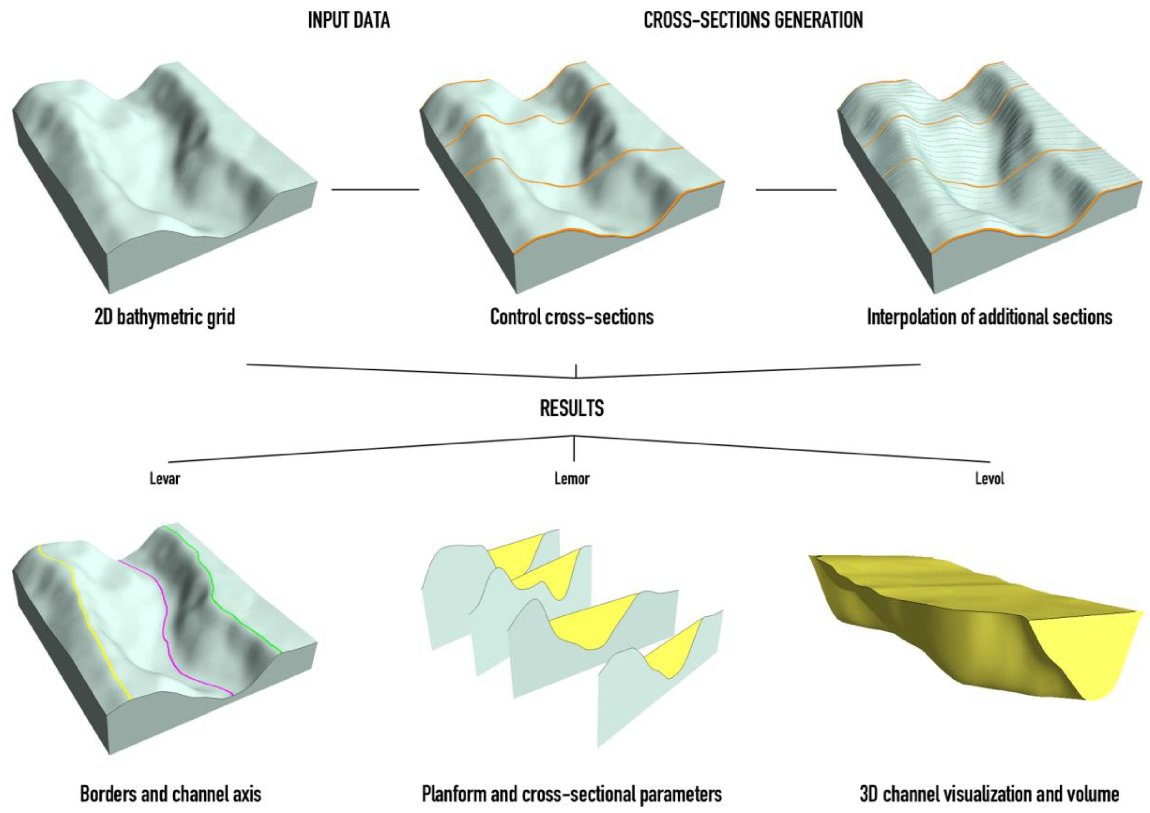
Figure 4.
Geometric parameters of the planform of a turbidite channel obtained by Lemor. CA: Channel area; CL: Channel length; VL: Valley length ; SI: Sinuosity index; CS: Channel slope axis; VS: Valley slope.
Figure 4.
Geometric parameters of the planform of a turbidite channel obtained by Lemor. CA: Channel area; CL: Channel length; VL: Valley length ; SI: Sinuosity index; CS: Channel slope axis; VS: Valley slope.
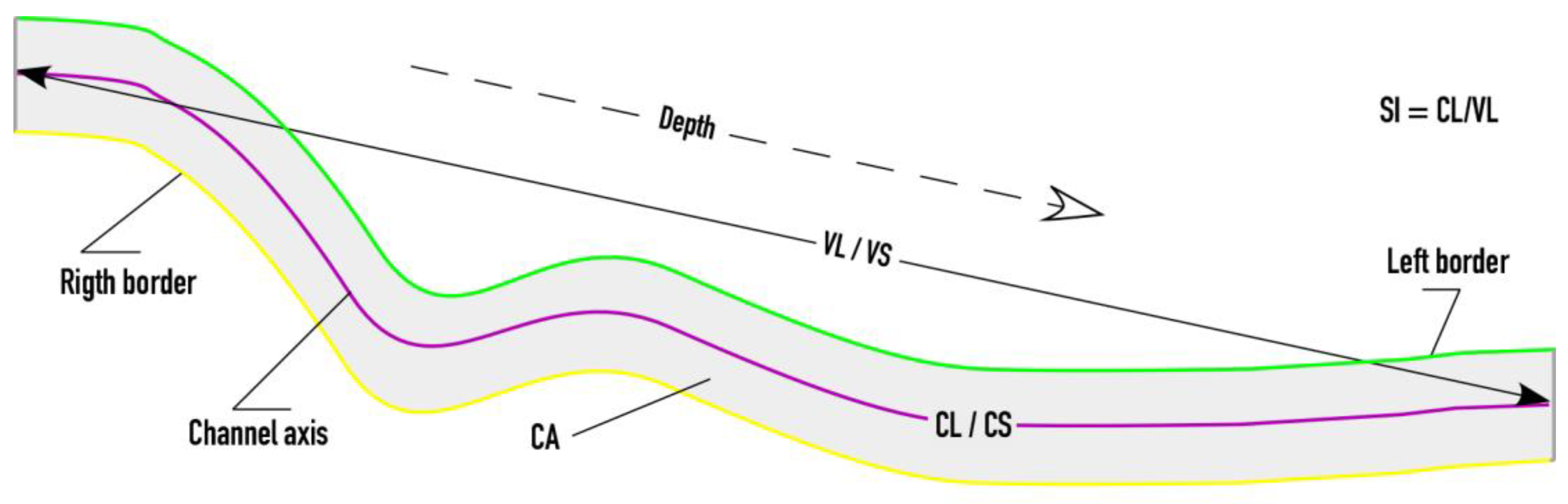
Figure 5.
Geometric parameters of the cross-section of a turbidite channel obtained by Lemor. DCA: Depth of the channel axis; DRL: Depth of the crest of the right levee; DLL: Depth of the crest of the left levee; HRF: Height of the right flank; HLF: Height of the left flank; AHF: Average height of flanks; HDF: Height difference between flanks ; CSW: Channel section width; CSA: Channel section area; WHR: Width to height ratio in the section.
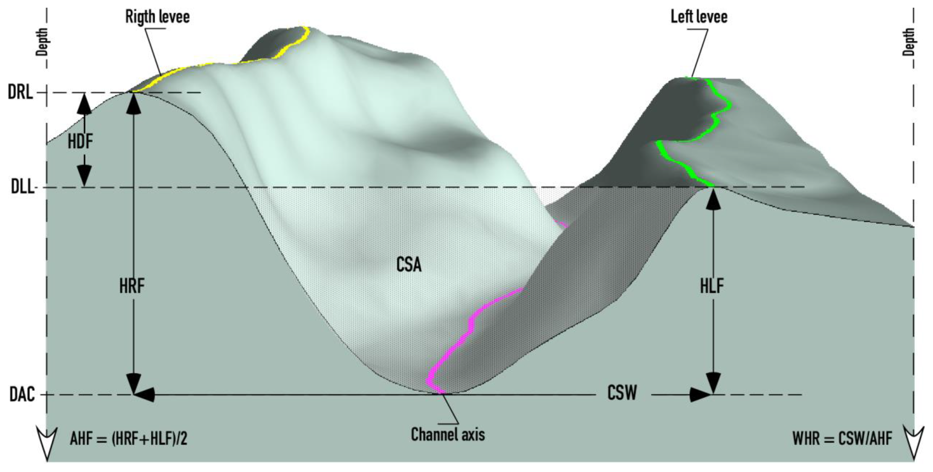
Figure 6.
A: Determination of the lines and dots (in blue) from which the surface representing the top of the channel is calculated. B: Example of the 3D visualization of the potential sedimentary fill of the channel.
Figure 6.
A: Determination of the lines and dots (in blue) from which the surface representing the top of the channel is calculated. B: Example of the 3D visualization of the potential sedimentary fill of the channel.
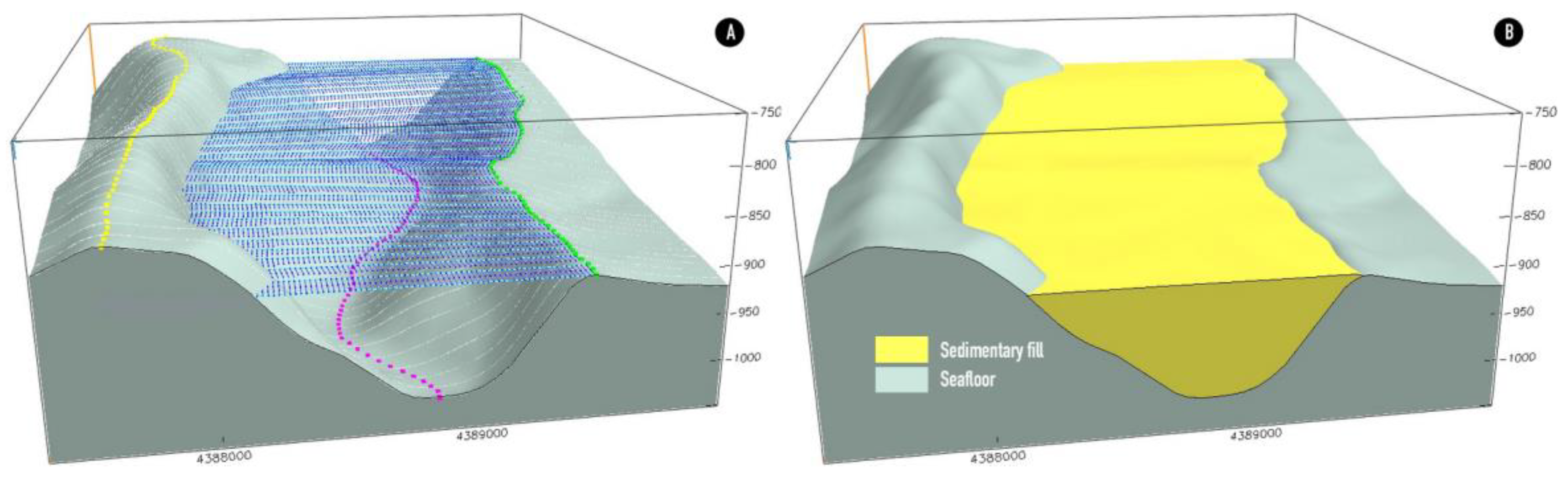
Figure 11.
Planform geometry of the CGC. The channel area and axis layout were created with Levar. CA: Channel area; CL: Channel length; VL: Length of the valley; SI: Sinuosity index; CS: Channel slope; VS: Valley slope.
Figure 11.
Planform geometry of the CGC. The channel area and axis layout were created with Levar. CA: Channel area; CL: Channel length; VL: Length of the valley; SI: Sinuosity index; CS: Channel slope; VS: Valley slope.
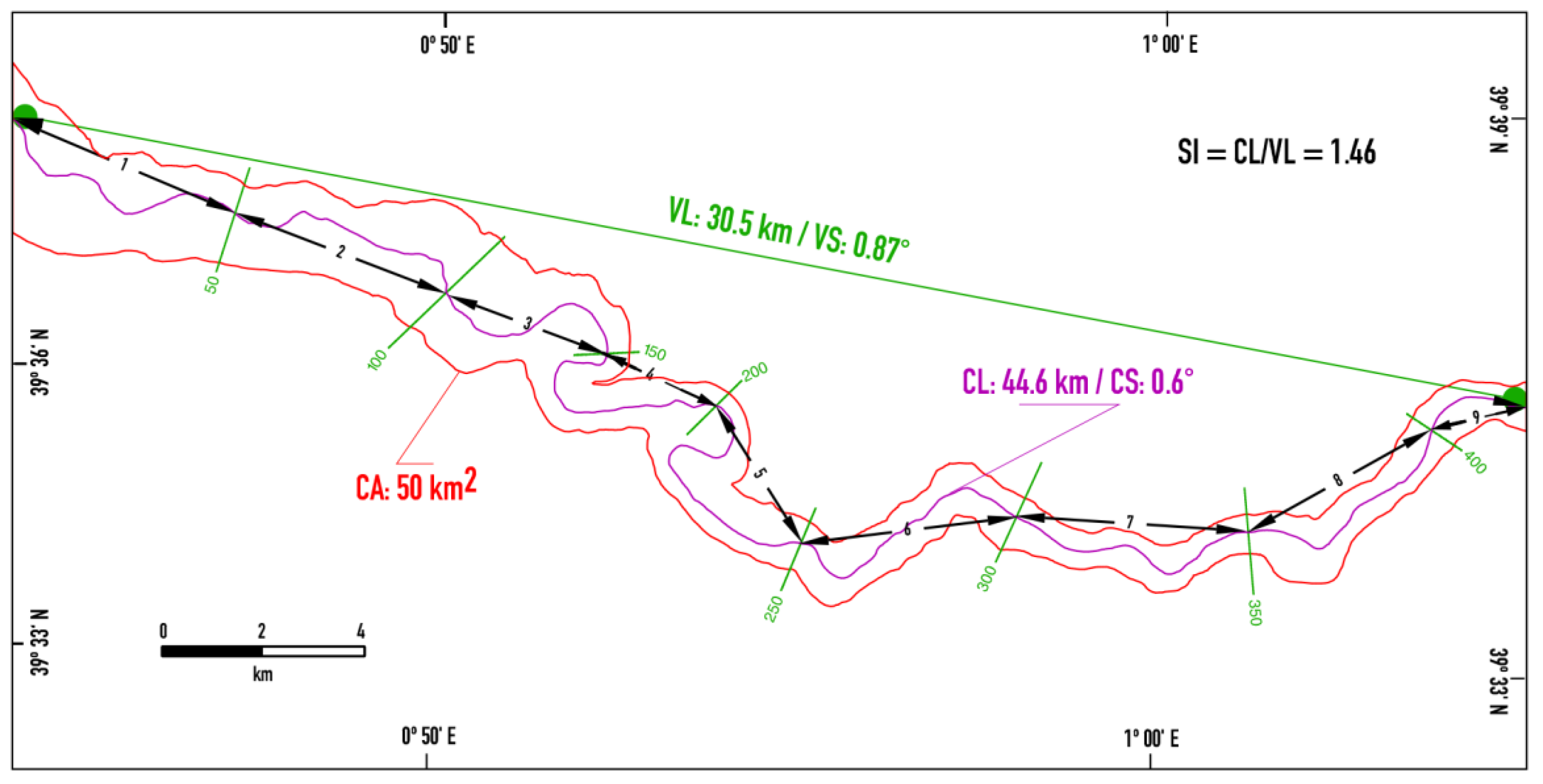
Figure 12.
A: Comparative graph of sinuosity and slope profiles along the CGC. The abscissa axis represents, at the bottom, the interpolated section number (ISN). The distance of the section from the beginning of the channel (SDC) is indicated at the top. On the axis of ordinates, the value in degrees of the slope of the channel (CS) and that of the valley (VS) is represented, and on the right, the sinuosity index (SI). B: Relationship between the CS, in degrees (upper abscissa) and in m/km (lower abscissa), and the SI. The line represents the best fit of the points.
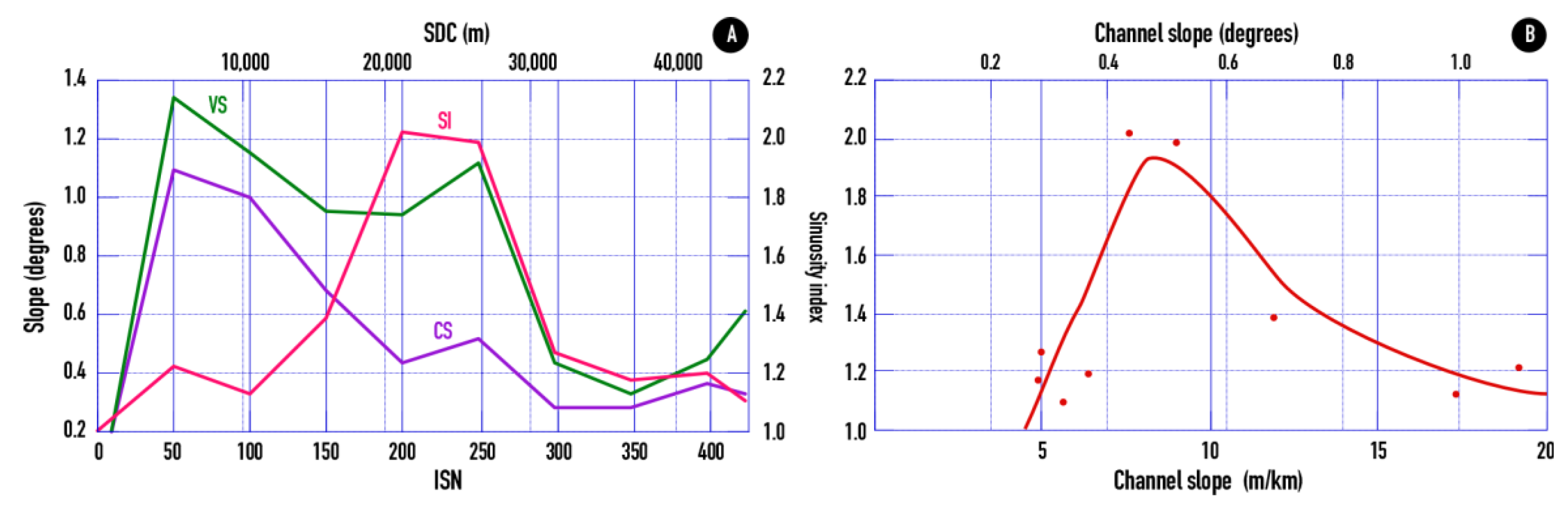
Figure 13.
Illustrative graphics, generated from cross-sectional data, of the geometry of the CGC. A: Depths of the axis channel and crests of the levees. B: Height of the flanks of the channel. C: Difference in height between the flanks of the channel. D: Width along the channel. E: Areas of the sections along the channel. F: Width-to-height ratio along the channel. The lower axis of abscissas is represented in all graphs by the interpolated section number (ISN). The upper axis of abscissas indicates the distances from the beginning of the channel (SDC). DCA: Depth of the channel axis; DRL: Depth of the crest of the right levee; DLL: Depth of the crest of the left levee; HRF: Height of the right flank; HLF: Height of the left flank; AHF: Average height of flanks; HDF: Height difference between flanks; CSW: Channel section width; CSA: Channel section area; WHR: Width to height ratio of the section.
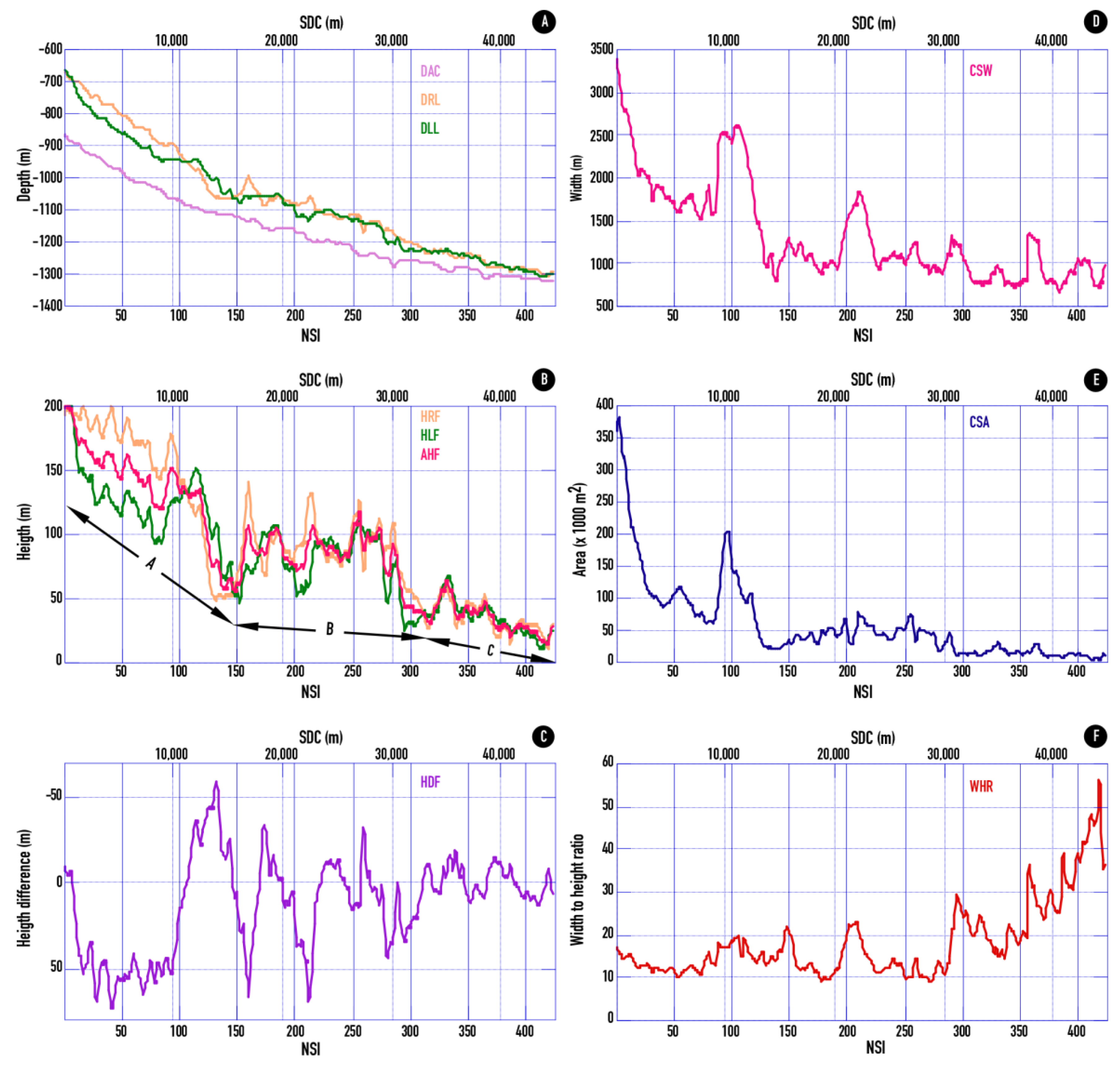
Figure 14.
3D view from the southwest of the potential sedimentary fill of the CGC. The calculated fill volume is indicated. Note the progressive decrease in channel size with depth. View inclination: 25°, vertical exaggeration: x5.
Figure 14.
3D view from the southwest of the potential sedimentary fill of the CGC. The calculated fill volume is indicated. Note the progressive decrease in channel size with depth. View inclination: 25°, vertical exaggeration: x5.
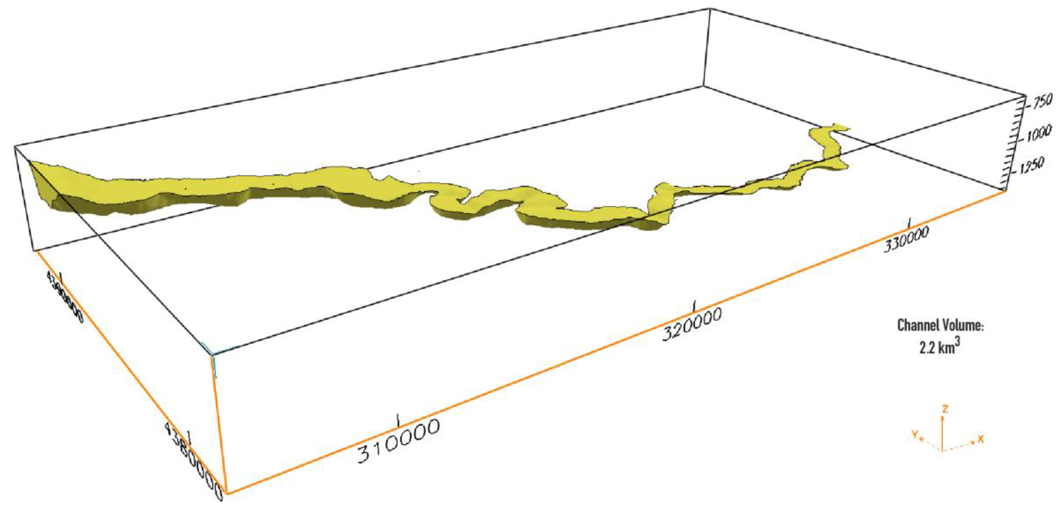

Table 1.
Planform parameters values for the entire channel and the reaches indicated in Figure 11. CL: Channel length; VL: Length of the valley; SI: Sinuosity index; CS: Channel slope; VS: Valley slope.
Table 1.
Planform parameters values for the entire channel and the reaches indicated in Figure 11. CL: Channel length; VL: Length of the valley; SI: Sinuosity index; CS: Channel slope; VS: Valley slope.
| Reach | CL (m) | VL (m) | SI | CS (°) | VS (°) |
|---|---|---|---|---|---|
| 1 | 5,896 | 4,840 | 1.22 | 1.10 | 1.33 |
| 2 | 5,181 | 4,607 | 1.12 | 0.99 | 1.15 |
| 3 | 4,481 | 3,228 | 1.39 | 0.68 | 0.94 |
| 4 | 4,912 | 2,431 | 2.02 | 0.43 | 0.93 |
| 5 | 6,413 | 3,229 | 1.99 | 0.51 | 1.11 |
| 6 | 5,371 | 4,247 | 1.26 | 0.28 | 0.44 |
| 7 | 5,328 | 4,559 | 1.17 | 0.28 | 0.32 |
| 8 | 4,891 | 4,098 | 1.19 | 0.36 | 0.44 |
| 9 | 2,198 | 2,001 | 1.10 | 0.32 | 0.61 |
| All channel | 44,671 | 30,540 | 1.46 | 0.59 | 0.87 |
Table 2.
Maximum, minimum, and average values for each cross-sectional parameter. DCA: Depth of the channel axis; DRL: Depth of the crest of the right levee; DLL: Depth of the crest of the left levee; HRF: Height of the right flank; HLF: Height of the left flank; AHF: Average height of flanks; HDF: Height difference between flanks ; CSW: Channel section width; CSA: Channel section area; WHR: Width to height ratio of the section.
| Cross-sections | DCA (m) |
DRL (m) |
DLL (m) |
HRF (m) |
HLF (m) |
AHF (m) |
HDF (m) |
CSW (m) |
CSA (m2) |
WHR |
|---|---|---|---|---|---|---|---|---|---|---|
| Maxim value | -865.6 | -673.3 | -663.7 | 198.9 | 202.0 | 200.1 | 73.9 | 3369 | 379058 | 55.91 |
| Mean value | -1165.0 | -1069.9 | -1082.8 | 95.1 | 82.2 | 88.7 | 12.9 | 1326 | 58547 | 17.97 |
| Minim value | -1327.8 | -1311.8 | -1309.7 | 10.4 | 11.5 | 13.2 | -58.1 | 659 | 3455 | 8.67 |
Disclaimer/Publisher’s Note: The statements, opinions and data contained in all publications are solely those of the individual author(s) and contributor(s) and not of MDPI and/or the editor(s). MDPI and/or the editor(s) disclaim responsibility for any injury to people or property resulting from any ideas, methods, instructions or products referred to in the content. |
© 2025 by the author. Licensee MDPI, Basel, Switzerland. This article is an open access article distributed under the terms and conditions of the Creative Commons Attribution (CC BY) license (https://creativecommons.org/licenses/by/4.0/).
Copyright: This open access article is published under a Creative Commons CC BY 4.0 license, which permit the free download, distribution, and reuse, provided that the author and preprint are cited in any reuse.


