
Submitted:
09 July 2025
Posted:
11 July 2025
You are already at the latest version
Abstract
The present work discusses the birth of the Universe via quantum tunneling through a potential barrier, based on quantum cosmology, taking into account a running cosmological constant. We consider the Friedmann-Lemaître-Robertson-Walker (FLRW) metric with positively curved spatial sections ($k = 1$) and the matter content is a dust perfect fluid. The model was quantized by the Dirac formalism, leading to a Wheeler-DeWitt equation. We solve that equation both numerically and using a WKB approximation. We studied the behavior of tunneling probabilities $TP_{WKB}$ and $TP_{int}$ by varying the energy $E$ of the dust perfect fluid, the phenomenological parameter $\nu$, the present value of the Hubble function $H_0$ and the constant energy density $\rho^0_\Lambda$, all the last three parameters associated with the time-varying cosmological constant.
Keywords:
quantum cosmology
; quantum tunneling process
; running cosmological constant
1. Introduction
One of the main problems faced by the Standard Model of Cosmology is the origin of spacetime through a big bang singularity. The existence of this singularity in the solutions to Einstein’s equations, when applied to cosmological models, highlights the importance of seeking a quantum gravity theory to eliminate it. Since the early Universe had dimensions much smaller than atomic nuclei, it is valid to suggest that it was governed by the laws of quantum mechanics. The first attempt to find a quantum gravity theory was the quantization of General Relativity, which gave rise to the Wheeler-DeWitt equation [1,2]. The application of this quantum theory to cosmology produced Quantum Cosmology (QC) [3]. Although it is widely accepted that QC is not the fundamental theory for describing the very early universe, many important results have already been obtained from the study of QC models. One of such results is the birth of the universe through a quantum tunneling process. Due to that process, it is possible to show that the universe may originate without the big bang singularity [4,5,6,7,8,9,10,11].
In the literature, there are many works using the quantum tunneling process in different quantum cosmology models [12,13,14,15,16,17,18,19,20,21]. In addition to the investigation of the quantum tunneling process, we may find several other recent works on different aspects of QC. In [22], the authors discuss the time in QC. It is shown that the reparametrization invariance is not guaranteed after one quantizes the model. Reference [23] shows a different quantization process, where the authors use what they call a "super field" consisting of the union of the spacetime wavefunction and the matter fields. The authors of [24] study how a form of dark energy called "phantom energy" affects the wavefunction of the universe which is a solution to the appropriate Wheeler-DeWitt equation. One of the most important results is that the higher the energy content in the model, the greater the probability that the universe will be born with a determined size, avoiding the initial singularity in . References [25,26,27] bring a novel approach in which the authors try to use fractional calculus in QC. In [28] the author reviews the DeBroglie-Bohm quantum theory. This is a theory that dispenses with the collapse of the wavefunction and, therefore, is quite appropriate to be applied to QC. In [29] the authors also address the issue of time not being an exactly defined notion in QC and present two solutions with applications focused on QC. In reference [30] the authors employ the fractional Riesz derivative in the Wheeler-DeWitt equation for a closed de Sitter geometry. The authors of [31] study a quantum cosmology model using electromagnetic radiation as a matter content. Reference [32] presents the first study of QC using quantum computers. There, the authors solve a Wheeler-DeWitt equation and show that the use of quantum computers allows one to reach solutions with a high degree of precision. In reference [33] the authors explore a two-dimensional cosmological model of quantum gravity. They do it, initially, by writing the classical sector with the aid of the ADM formalism, and then they solve the Wheeler-Dewitt equation in order to describe the quantum sector. In [34] the authors study approximate solutions to the Wheeler-DeWitt equation and compare the results with cosmological perturbative theories. In the work [35], the author works on the quantization of quantum cosmology models, introducing the concepts of mini-superspace, perfect fluids, and scalar fields, bringing up conceptual problems such as the evolution of time and unitarity, as well as physical interpretations. These are some examples showing that Quantum Cosmology is an active field and grows over time.
Since the seminal work by P. A. M. Dirac in 1937 [36] arguing about the possibility that some of the fundamental constants of nature may vary with the age of the Universe, many works have been done exploring that possibility. Although not mentioned in Dirac’s work, the cosmological constant (CC) is today a very important constant of nature because it is a possible candidate to explain the present accelerated expansion of our Universe [37,38]. Some recent observational evidence shows that the expansion of the universe accelerated faster in the past than it is doing now[39]. This opens up the possibility, among others, for a running CC. In fact, even before this recent observational evidence, several researchers have already considered the possibility of a running CC [40,41,42,43,44,45,46,47]. A promising line of investigation of a running CC is based on the study, using quantum field theory in curved spacetime, of the renormalization group (RG) [45,48,49,50,51,52]. In the RG method, the equation of state for the cosmological constant is exactly given by and the CC becomes time dependent. Also, using the RG method it is possible, with the aid of some cosmological observations, to impose phenomenological limits on a certain parameter of the method [51,53]. It certainly improves the predictions of this method.
In this work, we want to study the Universe in its early stages through quantum cosmology. For this purpose, the tunneling probabilities for the emergence of the Universe through a potential barrier are calculated. We do that with the help of the solutions to the Wheeler-DeWitt equation obtained in two different ways: the numerical solution and the WKB approximation. The Universe is described by a Friedmann-Lemaître-Robertson-Walker (FLRW) model with positive curvature of the spatial sections, coupled to a dust perfect fluid and a running cosmological constant, described by the RG method. The latter is introduced to describe the dark energy present in the Universe.
In Section 2, we derive the total Hamiltonian, draw a phase portrait, and solve the Hamilton equations for a FLRW cosmological model, with constant positive spatial sections and coupled to a dust perfect fluid and a running cosmological constant. In Section 3, we quantize the model and solve the resulting Wheeler-DeWitt equation, using a numerical method and the WKB approximation. In Section 4, we compute the WKB () and the integrated () tunneling probabilities for the universe to tunnel through the potential barrier. We investigate how and depend on several parameters of the model. Finally, in Section 5, we summarize the main points and results of the paper. In Appendix A, we compute in detail, with the aid of the Schutz variational formalism, the total Hamiltonian for the dust fluid.
2. The Classical Model
The classical cosmology, based on the FLRW model, has its foundations in Einstein’s General Theory of Relativity (GR) [54], accurately elucidating large-scale phenomena such as black holes, gravitational waves, light deflection, and the precession of Mercury’s orbit. Objectively, in this section, the ADM formalism [55,56] was used to derive the Hamiltonian density of GR, thus making possible to quantize it.
The action integral, written in terms of the matter Lagrangian density () and the Ricci scalar (R), is given by,
Where g is the determinant of the metric, is defined as the sum of the contributions from the time-varying CC, (where is the pressure associated to the time-varying CC), and the perfect fluid (where is the pressure associated to the fluid). In this work, the following system of units is used: .
If we introduce the values of R and , computed for the FLRW metric with positively curved spatial sections, in Equation (1) we obtain,
where is the scale factor, is the lapse function, is the time-varying CC energy density (we used that ), is the fluid energy density, is a constant associated with the fluid Equation (A5), the dot means derivative with respect to time and is defined as,
The running cosmological constant energy density, has the following expression [45,48,49,50,51,52],
where represents the vacuum energy density at present time, H is the Hubble function defined as , is a constant that gives the Hubble function at the present time, and the parameter is a dimensionless constant that emerges from the renormalization process and characterizes the magnitude of quantum effects on the vacuum energy density. It is defined as,
where represents the predominance of bosons () or fermions () at high energies, M is a weighted sum of the effective masses of massive virtual particles and is the Planck mass (). Since , the parameter is typically very small, of the order of [51,53]. This value reflects the low quantum contribution relative to the total gravitational energy. However, studies suggest that in the early Universe, during a highly anisotropic and dynamic phase, the usual limitations on the sign and magnitude of may not apply. In such conditions, could assume much larger values (both positive and negative). This occurs because spacetime conditions are dominated by intense quantum effects and high-energy interactions that influence vacuum dynamics [52]. This behavior enables exploration of cases where the values of directly impact the isotropization process and the evolution of the metric [52]. The parameter also regulates the temporal variation of the vacuum energy density.
Introducing the value of Equation (4) in the action Equation (2), we find,
From action (6) one extracts the following Lagrangian density,
for simplicity, we will consider .
Now we can compute the canonical momentum,
Introducing Equation (8) into the Hamiltonian density definition, and using the Schutz formalism [57], in order to determine the Hamiltonian of the matter sector (see Appendix A for more details), one obtains,
where . To avoid factor ordering ambiguities, one must use the following change of variables [58],
Choosing the gauge , the Hamiltonian density becomes,
Using the constraint equation one identifies the potential ,
which has the shape of a barrier. In Figure 1, we show an example of Equation (12), for , and . In this example, the maximum value of () is 14.1421.
The classical dynamics is governed by the Hamilton equations,
So, now one may impose the constraint equation leading to an equation for the momentum given by,
We begin studying the dynamics produced by Hamilton equations by constructing the phase portrait of the current model, which is shown in Figure 2. The curves are labeled according to the parameter , which takes the values , 1, 2, 5, 10, 14, , 15, 20, 25, …, 200, 250, 300. The phase portrait gives a general idea of all different types of dynamical solutions of the model. As we shall see next, all different types of dynamical solutions can be associated with the four regions identified in the phase portrait Figure 2.
After combining some of the Hamilton equations from Equation (13), one can obtain a second-order differential equation for the classical evolution of the scale factor,
When solving Equation (15), with the appropriate initial conditions, four different types of classical solutions are found pictured in Figure 3a,d. These solutions are: (i) A contraction solution which has x starting at a high value and decreasing until it reaches , which produces a big crunch singularity. This solution can be seen in Figure 3a. For this particular example, the initial conditions were and . These types of solutions are located in Region II of Figure 2; (ii) An expansion solution where x begins at small values and starts an expansion at an accelerated rate to infinity. This solution can be seen in Figure 3b. For this particular example, the initial conditions were and . These types of solution are located in Region I of Figure 2; (iii) An expansion followed by a contraction solution in which x begins at small values and grows until it reaches a maximum value. Then it begins to shrink until it reaches , which produces a big crunch singularity. This solution is shown in Figure 3c. For this particular example, the initial conditions were and . These types of solution are located in Region IV of Figure 2; (iv) A bouncing solution, where x starts at a high value, shrinks until it reaches a minimum value and then grows towards infinity. This solution is portrayed in Figure 3d. For this particular example, the initial conditions were and . These types of solution are located in Region III of Figure 2.
3. Canonical Quantization
The next step is the quantization of the present model. We shall do that following Dirac’s formalism [59,60], which consists of replacing the canonical variables x and T and their canonically conjugated momenta with its respective operators. After that, one must introduce the wavefunction of the Universe, which is a function of the operators associated with the canonical variables, written as . The quantum effects are prevailing in the early Universe and the wavefunction of the Universe, is responsible to describe those quantum effects. One initiates the quantization process by replacing the canonical momenta and with their respective operators:
Next, we must impose the constraint equation , where is the Hamiltonian operator. This equation gives rise to the Wheeler-DeWitt equation [1,2]. Using the Hamiltonian from Equation (9) with gauge choice and doing , one obtains the Wheeler-DeWitt equation for this model:
3.1. WKB Tunneling Probability
Assuming that one may write the solution to equation (17) in the form and using it in Equation (17), one finds,
with being given by Equation (12). Now, suppose that the WKB approximation is valid for the present model. Once obtained, the WKB solution will be used to calculate the tunneling probabilities through the potential barrier . Following the steps to obtain the WKB solution, one begins writing the solution as . Using this ansatz in equation (18) and assuming that is negligible compared to the other terms, the solution may be written as [61],
where and G are constants, is the value of x which the energy E intercepts the potential from the left side, and is the value of x where the energy E intercepts the potential from the right side. Also, the and terms are,
Using matrix notation, one can set forth the connection between coefficients and G [61],
The parameter gives the barrier height and length. It is given by,
Having the WKB solution, one is now able to compute the transmission coefficient, i.e., the tunneling probability. If one considers that there is no wave coming from the right (), the tunneling probability, being denoted by , will be [61],
For the present model, will be,
3.2. Integrated Tunneling Probability
The operator Equation (17) is self-adjoint [62] with respect to the internal product,
if the wavefunctions satisfy one of the next boundary conditions, or , where the prime ′ means the partial derivative with respect to x. In the present paper, we shall restrict our attention to wave functions satisfying . We also demand that when . Along with the WKB solution, we also solve the Wheeler-DeWitt equation (17) numerically. In order to do that, we employ a finite difference procedure based on the Crank-Nicolson method [63]. We tested the validity of our numerical solutions by computing the norm of the wavefunction for different times, and as a result, we found that it was always preserved. That test is commonly performed in order to evaluate the validity of numerical solutions to quantum mechanical systems [13,14,15,17]. The next step in order to solve the Wheeler-DeWitt equation Equation (17), is furnishing an initial wavefunction. That initial wavefunction fixes an energy for the dust. One may understand the relationship between the initial wavefunction energy and the dust energy because the time variable is related to the degree of freedom of the dust. Hence, the energies of the stationary states are associated with the energies of the dust fluid.
Among the several possibilities, as a matter of simplicity, we have chosen the following initial wavefunction,
where E represents the mean kinetic energy associated to the dust energy and is very concentrated in a region close to . The initial wavefunction Equation (26) must satisfy the following condition, in order to be normalized, . Since we want to calculate the tunneling probability, we must compute the outgoing wavefunction. In other words, we must compute the part of the wavefunction which tunnels the potential barrier. The outgoing wavefunction, propagates to infinity in the positive x direction, as time goes to infinity. Once we are performing a numerical calculation, we must specify a maximum value, in the x direction. Let us call that number . The behavior of all wavefunctions, we computed, and their time evolution show that they are well defined in the whole space.
Figure 4 gives an example of the probability density as a function of the scale factor x at the moment , when reaches the numerical infinity, at . In this example, we draw the potential written in Eq.(12), which is a barrier, with values , and . In this example, the maximum potential value is located at . The fluid energy is , which is smaller than . Then, for this example, the tunneling process will occur. For that fluid energy E, the wavefunction will reach the potential barrier at and, after tunneling, it will leave the potential barrier at .
In order to obtain the integrated tunneling probability, denoted by , we use the following definition [13,14],
Here, is the wavefunction of the universe calculated at the time , which is the moment reaches the numerical infinity . can be understood as the odds for the Universe to be found at the right side of the potential barrier.
4. Results
In this section we will compute the tunneling probabilities and for the potential given in Equation (12) and how they change due to variations of energy E and the parameters , and . Aiming to investigate the behavior of probabilities in the face of changes in parameters and energy, we fix them as well as the energy, except for the quantity under study. This strategy is applied to each one of the parameters and energy. The x values where the energy E intercepts the potential, and , are also relevant. They must be determined to calculate the probabilities.
4.1. The Phenomenological Parameter
To study how the tunneling probabilities and are affected by changes in the parameter, we fixed the values of parameters and and the energy E. We chose , and (this value is smaller than ). The range of values used to examine the behavior of and begin at and go all the way up to in steps of . Since the Universe under study is very primitive, may have negative or positive values. One can see the results of the calculations in Table 1 and Figure 5, which shows a comparison between and . As one can see, the change in is much more subtle than the change in . We have further analyzed each of the tunneling probabilities individually. It is possible to see in Figure 6 that both decrease when the parameter grows. Table 1 shows the parameter values, the tunneling probabilities and the x values where the energy intercepts the potential () from the left side () and from the right side ().
4.2. The Cosmological Constant Energy Density
To examine how the tunneling probabilities and are affected by changes in the parameter, we fixed values for parameters and and the energy E. Here, we chose , and (this value is smaller than ). The range of values used to examine the behavior of and begin at and go all the way up to in steps of . One can see the results of the calculations in Table 2 and Figure 7, which shows a comparison between and . Table 2 shows the parameter values, the tunneling probabilities and the x values where the energy intercepts the potential () from the left side () and from the right side (). Figure 7 shows that and increase as one increases the parameter .
4.3. Energy E
To study how the tunneling probabilities and are affected by changes in the fluid energy E, we fixed values for the potential barrier parameters. Here, we chose , and . The maximum value of this potential is . The energy values used to examine the behavior of and begin at and go all the way up to in steps of . We also include the values and . One can see the results of the calculations in Table 3 and Figure 8, which shows a comparison between and . Table 3 shows the energy values, the tunneling probabilities and the x values where the energy intercepts the potential () from the left side () and from the right side (). Figure 8 shows that and grow as one increases the energy.
4.4.
To examine how the tunneling probabilities and are affected by changes in the parameter, we fixed values for parameters and and determined a fixed energy value. Here, we chose , and (this value is smaller than ). The range of values used to examine the behavior of and begin at and go all the way up to in steps of . One can see the results of the calculations in Table 4 and Figure 9, which shows a comparison between and . Table 4 shows the parameter values, the tunneling probabilities and the x values where the energy intercepts the potential () from the left side () and from the right side (). Figure 9 shows that and decrease as one increases the parameter .
5. Conclusions
In the present work, the probability for the birth of a homogeneous and isotropic FLRW Universe with positively curved spatial sections () was studied. The matter content of the model is composed of a dust perfect fluid. The potential barrier of the model originates from the geometry of space-time, the fluid energy density and the presence of running cosmological constant, which can be interpreted as the zero-point energy of the quantum vacuum in Quantum Field Theory (QFT) [64]. The Hamiltonian was found using the ADM formalism and the model was quantized using the Dirac formalism.
We explicitly calculated the tunneling probabilities and for the birth of the Universe as a function of the phenomenological parameter (), the dust energy E, the cosmological constant energy density () and the Hubble parameter ().
It was observed that both tunneling probabilities, and , decrease as one increases . It was also noted that and grow as E increases, indicating that the Universe is more likely to be born with higher values of the dust energy E. The same is observed for the parameter, that is, and are bigger for higher values of . Finally, the tunneling probabilities decrease as one increases the value of .
So, the best conditions for the Universe to be born, in the present model, would be having the higher possible values for E and and the lowest possible values for and .
Author Contributions
All authors contributed to every stage of the paper, including the writing.
Funding
Not applicable in our research shown here
Institutional Review Board Statement
Not applicable in our research shown here.
Data Availability Statement
Not applicable in our research shown here
Acknowledgments
A. Corrêa Diniz thanks Coordenação de Aperfeiçoamento de Pessoal de Nível Superior (CAPES) for his scholarship. A. O. Castro Junior thanks UERJ and CAPES (Finance Code 001) for financial support. G. Oliveira-Neto thanks FAPEMIG (APQ-06640-24) for partial financial support. G. A. Monerat thanks FAPERJ for partial financial support and Universidade do Estado do Rio de Janeiro, UERJ, for the Prociência grant.
Conflicts of Interest
Not applicable in our research shown here
Appendix A. Schutz Formalism
According to Schutz variational formalism for FLRW cosmological models [57], the fluid’s 4-velocity is written in terms of the thermodynamical potentials and S:
where is the specific enthalpy, S is the specific entropy and the potentials and have no clear physical meaning. Also, the normalization condition for this 4-velocity is
Using Equation (A2) and a coordinate system comoving with the fluid, we may write Equation (A1) in the following way,
The action for the fluid is [57],
where p is the fluid pressure. In the case of a perfect fluid that satisfies an equation of state,
where is a constant and is the fluid energy density. It is possible to show, with the aid of some thermodynamic equations, that p may be written in the following form,
The value of the quantity , for the FLRW metric is given by: . Now, introducing that value along with the values of p Equation (A6) and Equation (A3) in (A4), one obtains the following value for the Lagrangian density of the fluid (),
From the above Lagrangian density Equation (A7), we may compute the conjugated momenta and ,
The Hamiltonian density of the matter () is obtained with the aid of the Equation (A7), the momenta and . It has the expression,
In order to simplify Equation (A9), we introduce the canonical transformations [10],
With these transformations, Equation (A9) takes the form,
Finally, in the specific case of dust we have and such that the fluid’s Hamiltonian density is reduced to
References
- B. S. DeWitt, Quantum Theory of Gravity. I. The Canonical Theory. Physical Review 1967, 160, 1113–1148. [CrossRef]
- J. A. Wheeler, SUPERSPACE AND THE NATURE OF QUANTUM GEOMETRODYNAMICS, Battelle Rencontres, pp. 242–307, 1968. https://www.osti.gov/biblio/4124259.
- P. V. Moniz, Quantum Cosmology - The Supersymmetric Perspective - vol. 1: Fundamentals, Lecture Notes in Physics, vol. 803, Springer, Berlin Heidelberg, 2010.
- L. P. Grishchuk and Ya. B. Zeldovich, Quantum Structure of Space and Time, eds. M. Duff and C. Isham, Cambridge University Press, Cambridge, 1982.
- A. Vilenkin, Creation of Universes from Nothing, Physics Letters B, vol. 117, p. 25, 1982.
- A. Vilenkin, Quantum Creation of Universes, Physical Review D, vol. 30, p. 509, 1984.
- A. Vilenkin, Boundary Conditions in Quantum Cosmology, Physical Review D, vol. 33, p. 3560, 1986.
- J. B. Hartle and S. W. Hawking, Wave Function of the Universe, Physical Review D, vol. 28, p. 2960, 1983.
- A. D. Linde, Quantum Creation of the Inflationary Universe, Lettere al Nuovo Cimento, vol. 39, p. 401, 1984.
- V. A. Rubakov, Quantum Mechanics in the Tunneling Universe, Physics Letters B, vol. 148, p. 280, 1984.
- A. Vilenkin, Quantum cosmology and eternal inflation, in The future of theoretical physics and cosmology, eds. G. W. Gibbons, E. P. S. Shellard, and S. J. Rankin, pp. 649–666, Cambridge University Press, Cambridge, 2003.
- M. Bouhmadi-Lopez and P. V. Moniz, FRW quantum cosmology with a generalized Chaplygin gas, Physical Review D, vol. 71, p. 063521, 2005.
- J. Acacio de Barros, E. V. Corrêa Silva, G. A. Monerat, G. Oliveira-Neto, L. G. Ferreira Filho, and P. Romildo Jr., Tunneling probability for the birth of an asymptotically DeSitter universe, Physical Review D, vol. 75, p. 104004, 2007.
- G. A. Monerat, G. Oliveira-Neto, E. V. Corrêa Silva, L. G. Ferreira Filho, P. Romildo Jr., J. C. Fabris, R. Fracalossi, S. V. B. Gonçalves, and F. G. Alvarenga, The dynamics of the early universe and the initial conditions for inflation in a model with radiation and a Chaplygin gas, Physical Review D, vol. 76, p. 024017, 2007.
- G. A. Monerat, C. G. M. Santos, G. Oliveira-Neto, E. V. Corrêa Silva, and L. G. Ferreira Filho, The dynamics of the early universe in a model with radiation and a generalized Chaplygin gas, European Physical Journal Plus, vol. 136, p. 34, 2021.
- G. A. Monerat, F. G. Alvarenga, S. V. B. Gonçalves, G. Oliveira-Neto, C. G. M. Santos, and E. V. Corrêa Silva, The effects of dark energy on the early Universe with radiation and an ad hoc potential, European Physical Journal Plus, vol. 137, p. 117, 2022.
- N. M. N da Rocha, G. A. Monerat, F. G. Alvarenga, S. V. B. Gonçalves, G. Oliveira-Neto, E. V. Corrêa Silva, and C. G. M. Santos, Early universe with dust and Chaplygin gas, European Physical Journal Plus, vol. 137, p. 1103, 2022.
- G. Oliveira-Neto, D. L. Canedo, and G. A. Monerat, Tunneling probabilities for the birth of universes with radiation, cosmological constant and an ad hoc potential, European Physical Journal Plus, vol. 138, p. 400, 2023.
- A. Oliveira Castro Junior, G. Oliveira-Neto, and G. A. Monerat, Primordial dust universe in the Horava-Lifshitz theory, Modern Physics Letters A, vol. 39, nos. 23 and 24, p. 2450112, 2024.
- A. Oliveira Castro Junior, G. Oliveira-Neto, and G. A. Monerat, The initial moments of a Ho?ava-Lifshitz cosmological model, General Relativity and Gravitation, vol. 56, p. 125, 2024.
- G. A. Monerat, H. J. Brumatto, G. Oliveira-Neto, F. G. Alvarenga, E. V. Corrêa Silva, and A. L. B. Ribeiro, Non-singular birth of the universe: High-performance numerical solutions of the Wheeler-DeWitt equation, Physics Letters B, vol. 868, p. 139623, 2025.
- M. Bojowald and T. Halnon, Time in quantum cosmology, Physical Review D, vol. 98, no. 6, p. 066001, 2018.
- S. J. Robles-Pérez, Quantum cosmology in the light of quantum mechanics, Galaxies, vol. 7, no. 2, p. 50, 2019.
- C. R. Muniz, M. S. Cunha, V. B. Bezerra, and H. S. Vieira, A cosmologia quântica de wheeler-dewitt e o universo despedaçado, Conexões-Ciência e Tecnologia, vol. 13, no. 2, pp. 70–76, 2019.
- P. V. Moniz and S. Jalalzadeh, From fractional quantum mechanics to quantum cosmology: an overture, Mathematics, vol. 8, no. 3, p. 313, 2020.
- S. M. M. Rasouli, S. Jalalzadeh, and P. V. Moniz, Broadening quantum cosmology with a fractional whirl, Modern Physics Letters A, vol. 36, no. 14, p. 2140005, 2021.
- D. L. Canedo, P. Moniz, and G. Oliveira-Neto, Quantum Creation of a Friedmann-Robertson-Walker Universe: Riesz Fractional Derivative Applied, Fractal and Fractional, vol. 9, p. 349, 2025.
- N. Pinto-Neto, The de Broglie-Bohm quantum theory and its application to quantum cosmology, Universe, vol. 7, no. 5, p. 134, 2021.
- C. Kiefer and P. Peter, Time in quantum cosmology, Universe, vol. 8, no. 1, p. 36, 2022.
- S. Jalalzadeh, E. W. Oliveira Costa, and P. V. Moniz, de Sitter fractional quantum cosmology, Physical Review D, vol. 105, no. 12, p. L121901, 2022.
- S. Jalalzadeh, A. Mohammadi, and D. Demir, A quantum cosmology approach to cosmic coincidence and inflation, Physics of the Dark Universe, vol. 40, p. 101227, 2023.
- C. C. E. Wang and J. H. P. Wu, Quantum Cosmology on Quantum Computer, arXiv preprint gr-qc:2410.22485, 2024. https://arxiv.org/abs/2410. 2248.
- D. Anninos, C. Baracco, and B. Mühlmann, Remarks on 2D quantum cosmology, Journal of Cosmology and Astroparticle Physics, vol. 2024, no. 10, p. 031, 2024.
- F. Piazza and S. Vareilles, Cosmological perturbations meet Wheeler DeWitt, arXiv preprint gr-qc:2412.19782, 2024.
- S. Gielen, Quantum Cosmology, in Encyclopedia of Mathematical Physics, Elsevier, pp. 520–530, 2025. [CrossRef]
- P. A. M. Dirac, The Cosmological Constants, Nature, vol. 139, p. 323, 1937.
- A. G. Riess et al., Observational Evidence from Supernovae for an Accelerating Universe and a Cosmological Constant, Astronomical Journal, vol. 116, p. 1009, 1998.
- S. Perlmutter et al., Measurements of ω and λ from 42 High-Redshift Supernovae, Astrophysical Journal, vol. 517, p. 565, 1999.
- M. Cortes and A. R. Liddle, Interpreting DESI’s evidence for evolving dark energy, Journal of Cosmology and Astroparticle Physics, vol. 12, p. 007, 2024.
- P. J. E. Peebles and Bharat Ratra, COSMOLOGY WITH A TIME-VARIABLE COSMOLOGICAL "CONSTANT", Astrophysical Journal, vol. 325, pp. L17–L20, 1988.
- W. Chen and Y. S. Wu, Implications of a cosmological constant varying as R-2, Physical Review D, vol. 41, p. 695, 1990.
- J. C. Carvalho, J. A. S. Lima, and I. Waga, Cosmological consequences of a time-dependent λ term, Physical Review D, vol. 46, p. 2404, 1992.
- B. Ratra and A. Quillen, Gravitational lensing effects in a time-variable cosmological "constant" cosmology, Monthly Notices of the Royal Astronomical Society, vol. 259, pp. 738–742, 1992.
- A. A. Starobinsky, How to determine an effective potential for a variable cosmological term, JETP Letters, vol. 68, p. 757, 1998.
- I. L. Shapiro and J. Sola, On the scaling behavior of the cosmological constant and the possible existence of new forces and new light degrees of freedom, Physics Letters B, vol. 475, p. 236, 2000.
- T. Padmanabhan, Cosmological constant and the weight of the vacuum, Physics Reports, vol. 380, pp. 235–320, 2003.
- C. P. Singh and Suresh Kumar, Bianchi Type-1 Space-Time with Variable Cosmological Constant, International Journal of Theoretical Physics, vol. 47, pp. 3171–3179, 2008.
- I. L. Shapiro and J. Sola, The scaling evolution of the cosmological constant, Journal of High Energy Physics, 2002.
- I. L. Shapiro, J. Sola, C. España-Bonet, and P. Ruiz-Lapuente, Variable cosmological constant as a Planck scale effect, Physics Letters B, vol. 574, 2003. [CrossRef]
- C. España-Bonet, P. Ruiz-Lapuente, I. L. Shapiro, and J. Sola, Testing the running of the cosmological constant with type Ia supernovae at high z, Journal of Cosmology and Astroparticle Physics, vol. JCAP02, p. 006, 2004. [CrossRef]
- J. C. Fabris, I. L. Shapiro, and J. Sola, On the cosmological constant and the Einstein field equations, JCAP, vol. 02, p. 016, 2007. [CrossRef]
- V. G. Oliveira, G. Oliveira-Neto, and I. L. Shapiro, Kantowski-Sachs Model with a Running Cosmological Constant and Radiation, Universe, vol. 10, p. 83, 2024.
- J. A. Agudelo Ruiz, T. de Paula Netto, J. C. Fabris, and I. L. Shapiro, Primordial universe with the running cosmological constant, European Physical Journal C, vol. 80, p. 851, 2020.
- Ray D’Inverno. Introducing Einstein’s Relativity, 2020.
- Arnowitt, R. , Deser, S., Misner, C. W., The Dynamics of General Relativity in Gravitation: an introduction to current research, arXiv:gr-qc/0405109, Wiley, New York, 1962.
- C. W. Misner ; K. S. Thorne and J. A. Wheeler, Gravitation, 1973.
- B. F. Schutz, Perfect Fluids in General Relativity: Velocity Potentials and a Variational Principle, Physical Review, 1970.
- M. J. Gotay and J. Demaret, Quantum cosmological singularities, Physical Review D, vol. 28, p. 2402, 1983.
- P. A. M. Dirac, Generalized Hamiltonian Dynamics, Canadian Journal of Mathematics, Cambridge University Press, 1950.
- P. A. M. Dirac, Lectures on Quantum Mechanics, Belfer Graduate School of Science Monographs Series, Dover, 1964.
- E. Merzbacher, Quantum Mechanics, Wiley, 1970.
- N. A. Lemos, Radiation?dominated quantum Friedmann models, J. Math. Phys., 1996.
- J. Crank and P. Nicolson, A practical method for numerical evaluation of solutions of partial differential equations of the heat-conduction type, Proc. Cambridge Philos. Soc., 1947.
- S. M. Carroll, The Cosmological Constant, Living Reviews in Relativity, vol. 4, p. 1, 2001. [CrossRef]
Figure 1.
Potential with , and .
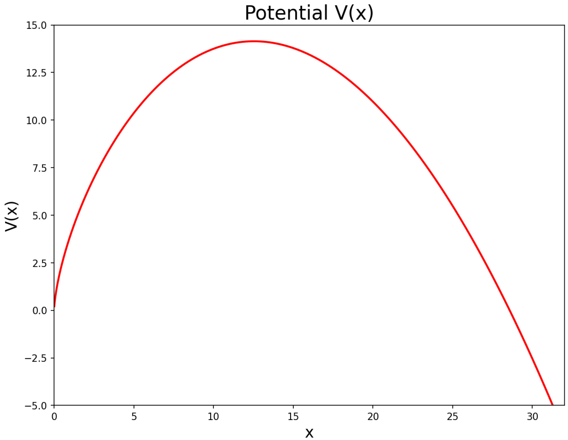
Figure 2.
Phase portrait of the model made with the potential values , and , while the parameter takes different values. The dashed line occurs when and is called the separatrix.
Figure 2.
Phase portrait of the model made with the potential values , and , while the parameter takes different values. The dashed line occurs when and is called the separatrix.
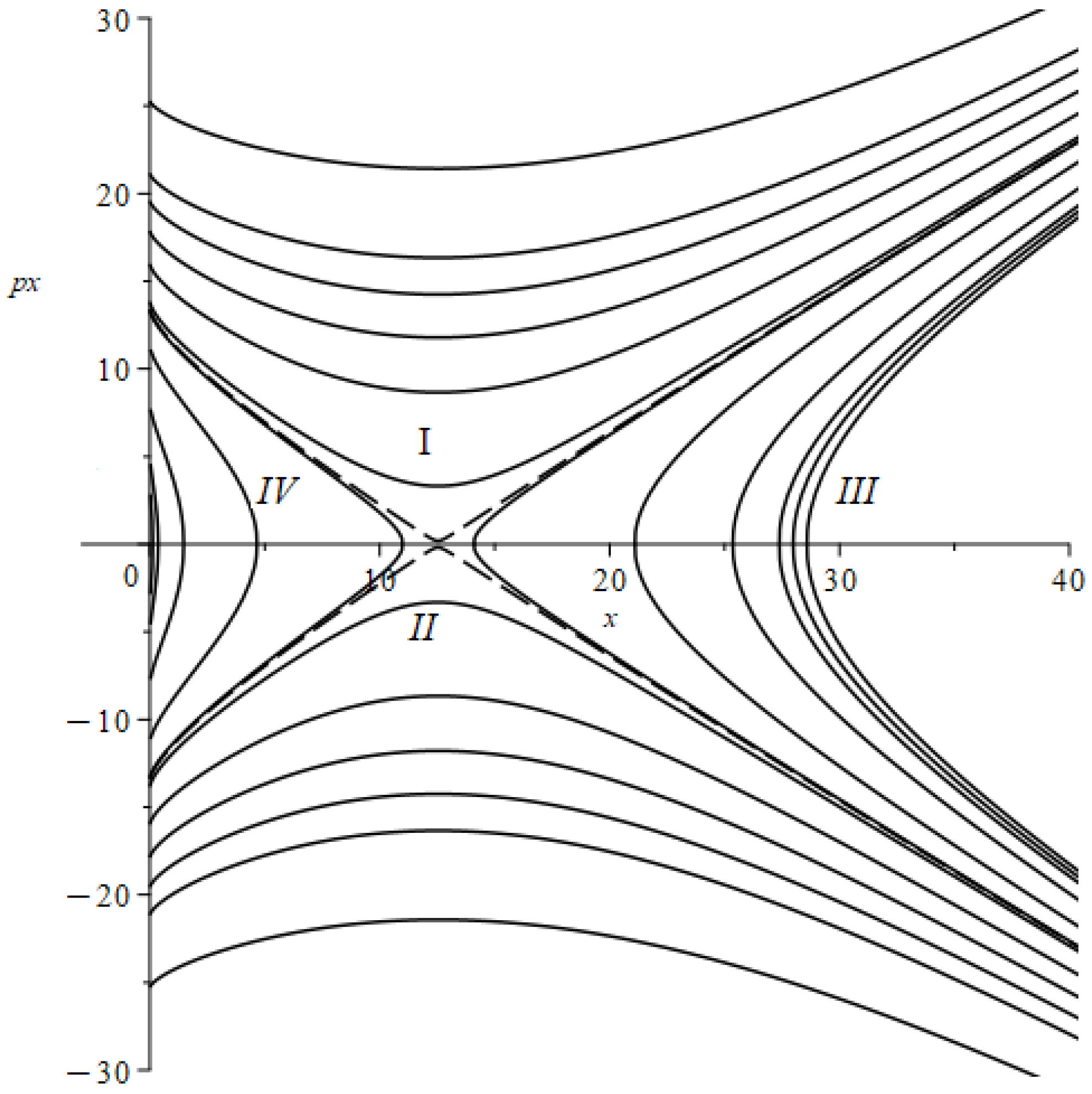
Figure 3.
Figure 3a shows a contraction solution, where x begins at a higher value and decreases to . Figure 3b depicts an expanding solution, where x begins at lower value and expands towards infinity. Figure 3c shows an expansion followed by a contraction. Figure 3d shows a bouncing solution, where x starts at a high value, shrinks to a minimum and begins an expansion immediately to infinity.
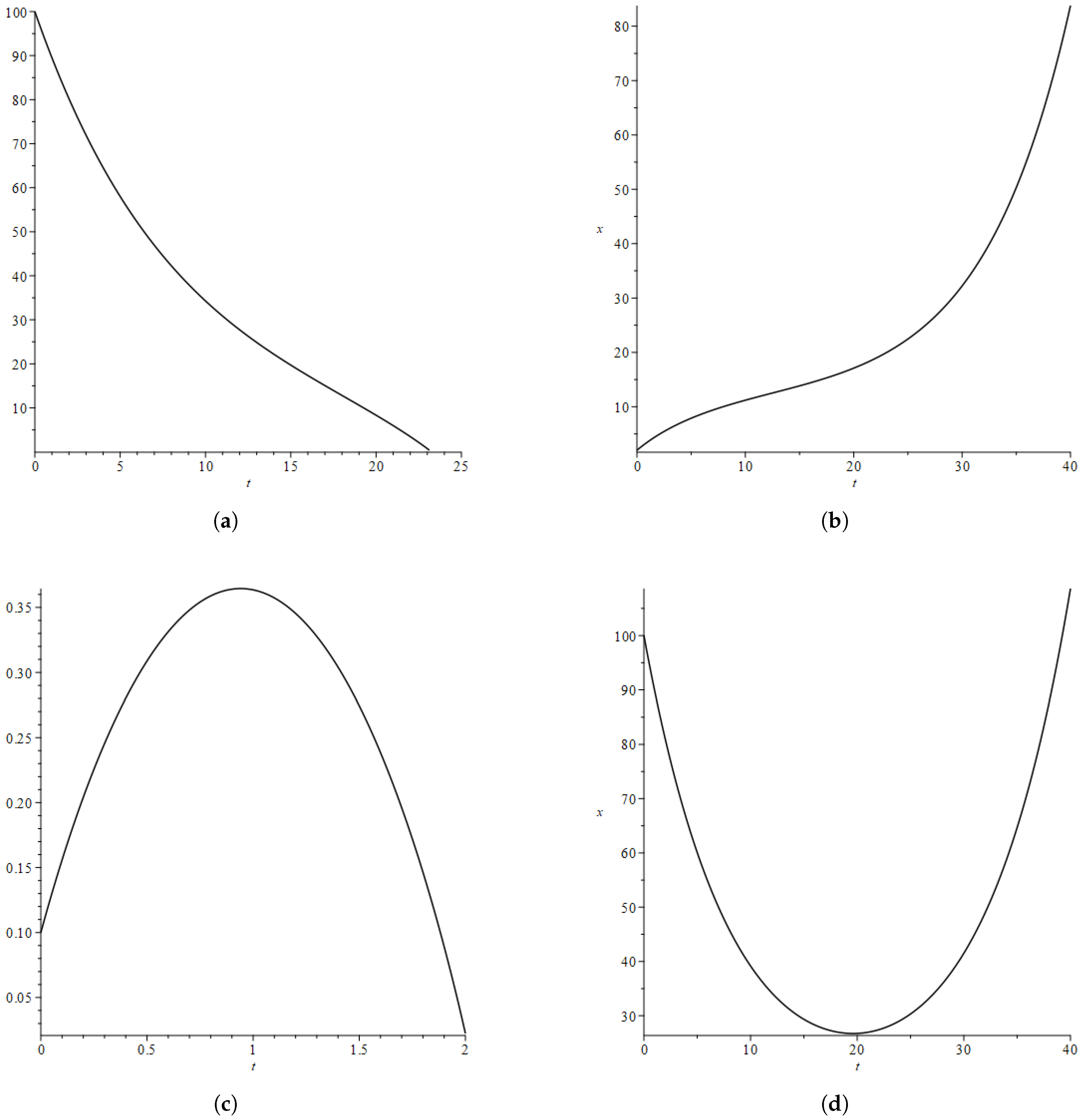
Figure 4.
for , , , at the moment , when reaches the numerical infinity, defined as .
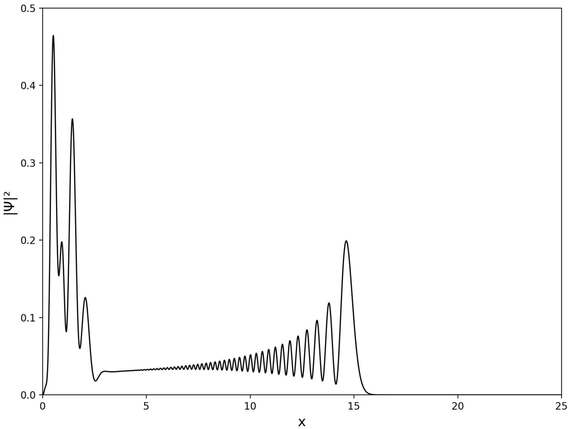
Figure 5.
Comparison between (solid line) and (dots) as changes for a simulation time and fixed energy . changes more slowly compared to and this gives the impression of being almost a constant line.
Figure 5.
Comparison between (solid line) and (dots) as changes for a simulation time and fixed energy . changes more slowly compared to and this gives the impression of being almost a constant line.
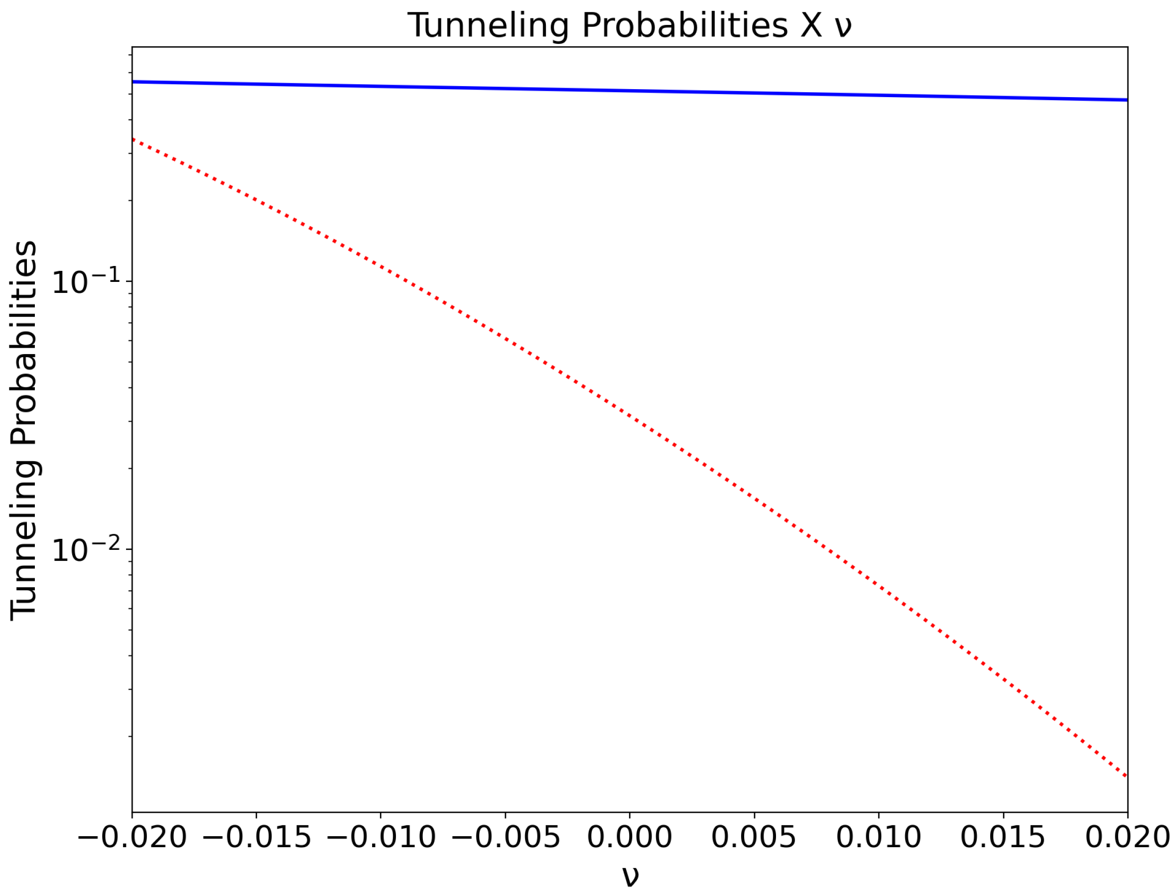
Figure 6.
Individual comparison of (a) and (b) as changes for a simulation time and fixed energy . Here one can see that both decrease as increases.
Figure 6.
Individual comparison of (a) and (b) as changes for a simulation time and fixed energy . Here one can see that both decrease as increases.
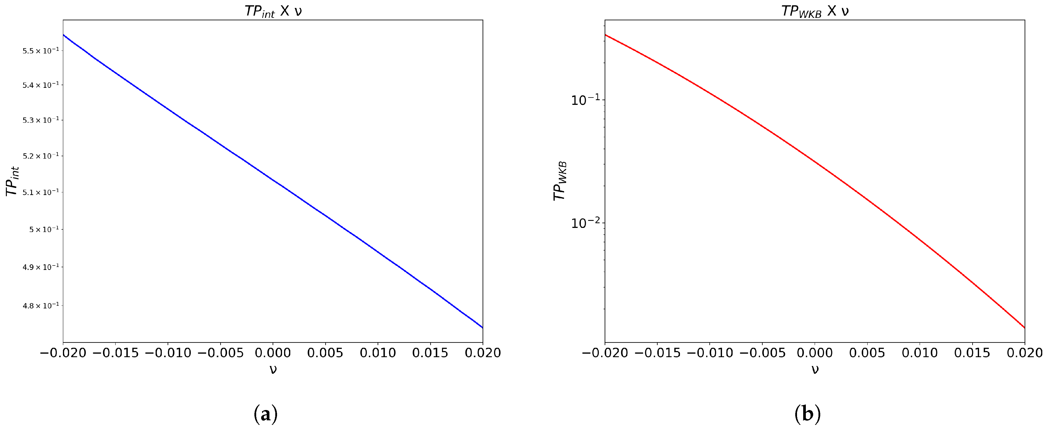
Figure 7.
Comparison of (solid line) and (dots) as changes for a simulation time and fixed energy .
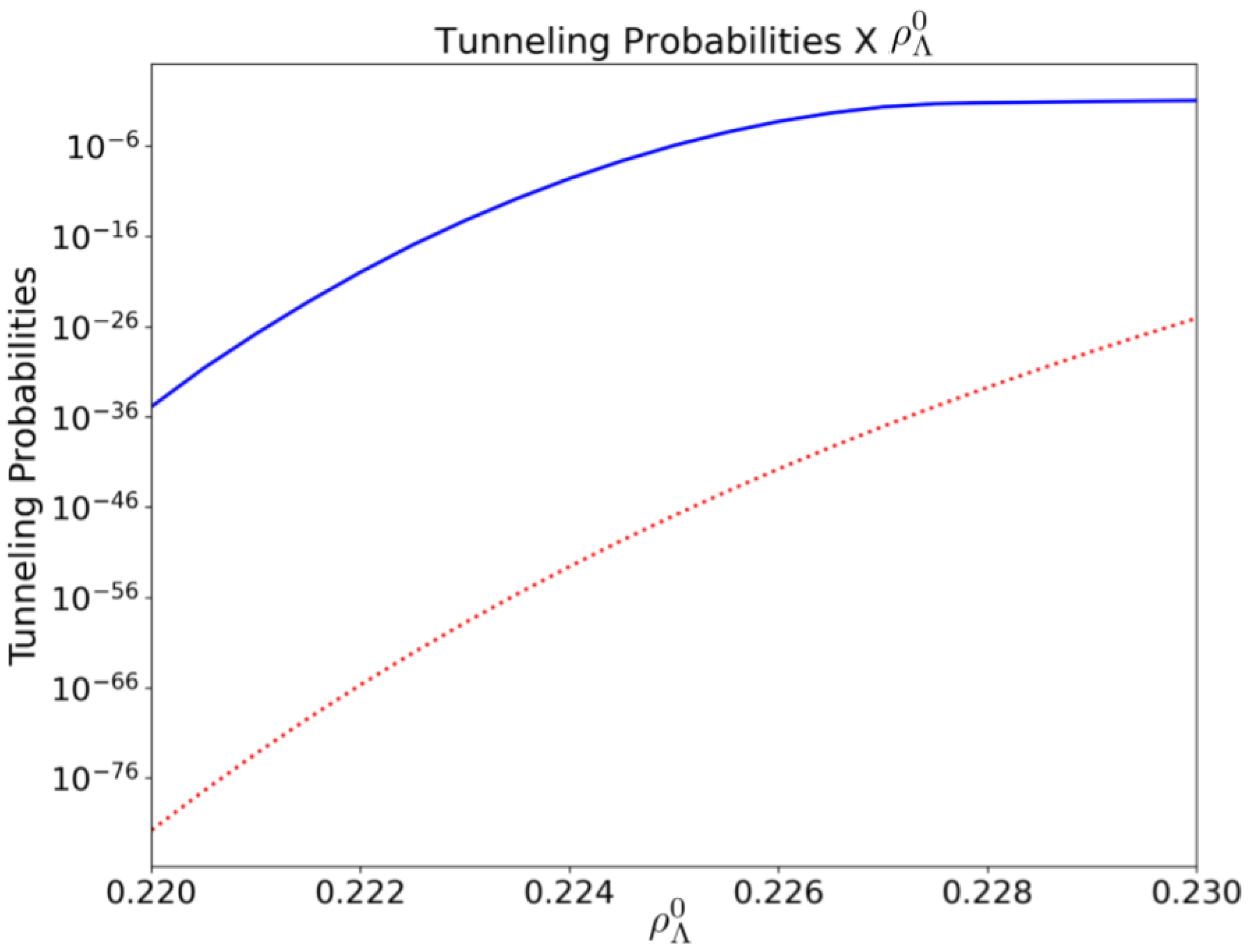
Figure 8.
Comparison of (solid line) and (dots) as energy E changes for a simulation time .
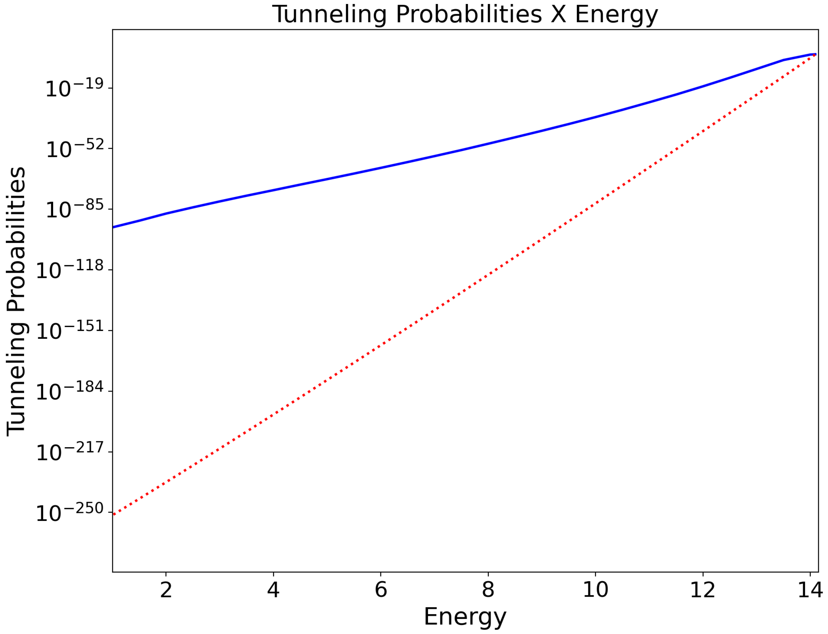
Figure 9.
Comparison of (solid curve) and (dots) as changes for a simulation time and fixed energy .
Figure 9.
Comparison of (solid curve) and (dots) as changes for a simulation time and fixed energy .
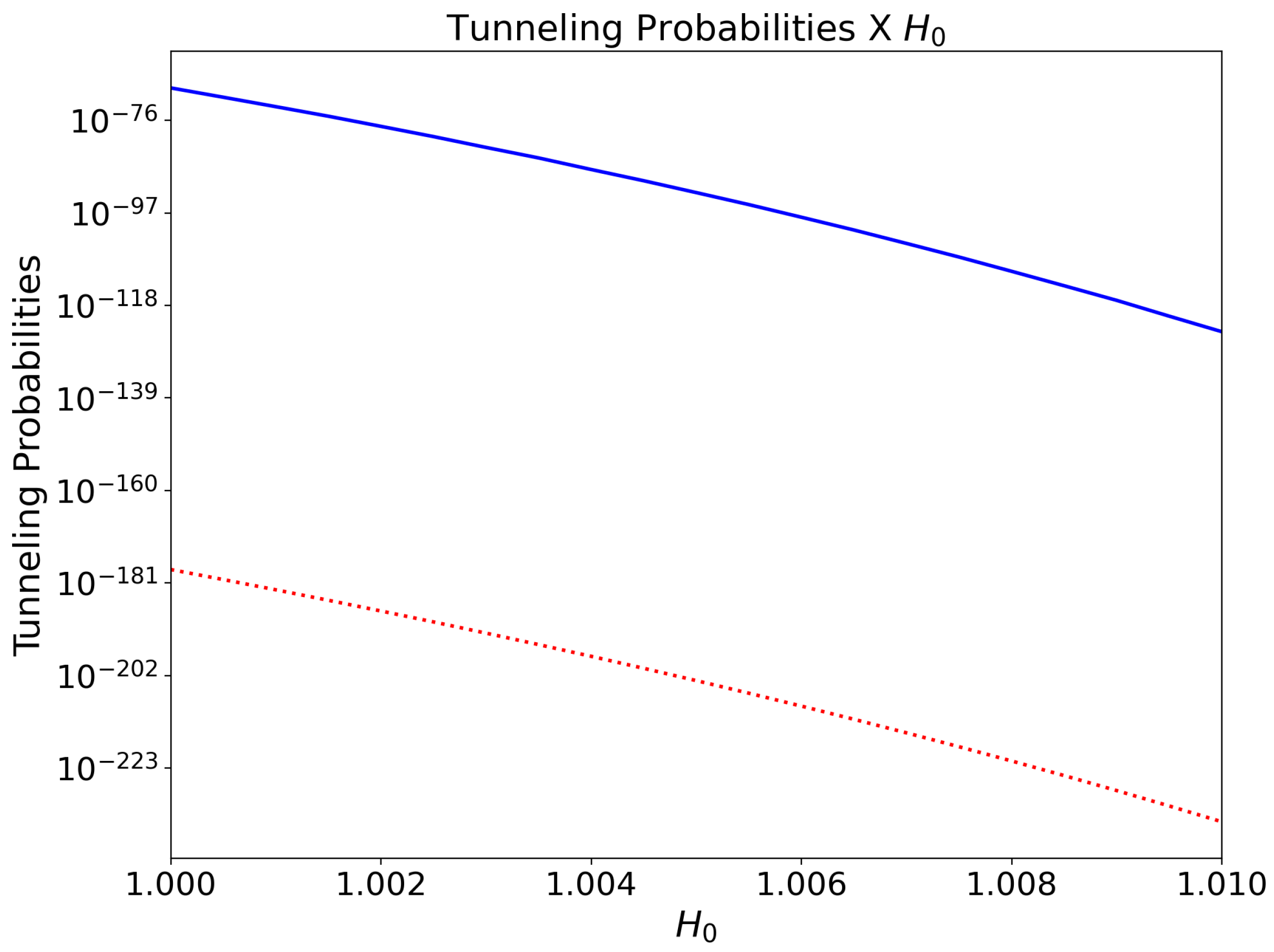

Table 1.
Variation of and as grows with a simulation time and a fixed energy .
Table 2.
Variation of and as grows with a simulation time and a fixed energy .
Table 3.
The variation of and as E changes for a simulation time .
| Energy | ||||
|---|---|---|---|---|
Table 4.
Variation and as grows with a simulation time and a fixed energy .
Disclaimer/Publisher’s Note: The statements, opinions and data contained in all publications are solely those of the individual author(s) and contributor(s) and not of MDPI and/or the editor(s). MDPI and/or the editor(s) disclaim responsibility for any injury to people or property resulting from any ideas, methods, instructions or products referred to in the content. |
© 2025 by the authors. Licensee MDPI, Basel, Switzerland. This article is an open access article distributed under the terms and conditions of the Creative Commons Attribution (CC BY) license (http://creativecommons.org/licenses/by/4.0/).
Copyright: This open access article is published under a Creative Commons CC BY 4.0 license, which permit the free download, distribution, and reuse, provided that the author and preprint are cited in any reuse.


