
Submitted:
24 June 2025
Posted:
10 July 2025
You are already at the latest version
Abstract
This review investigates the application of unsupervised machine learning algorithms to astronomical data. Unsupervised machine learning enables the researchers to analyze large, high-dimensional, and unlabeled data sets and is sometimes considered more helpful for exploratory analysis because it is not limited by present knowledge and can therefore be used to extract new knowledge. Unsupervised machine learning algorithms that have been repeatedly applied to analyze astronomical data are classified according to their usage, including clustering, dimension reduction, and neural network models. This review also discusses anomaly detection and symbolic regression. For each algorithm, this review discusses the algorithm's functioning in mathematical and statistical terms, the algorithm's characteristics (e.g., advantages and shortcomings, possible types of inputs), and the different types of astronomical data analyzed with the algorithm. Example figures are generated. This review aims to provide an up-to-date overview of both the high-level concepts and detailed applications of various unsupervised learning methods in astronomy, highlighting their advantages and disadvantages to help researchers new to unsupervised learning.
Keywords:
unsupervised machine learning
; data analysis
; astronomy
; artificial intelligence
1. Introduction
Machine learning (ML) has been applied to various analyses of astronomical data, such as analyzing spectral data e.g., [1,2,3], catalogs e.g., [4,5,6], light curves e.g., [7,8,9], and images e.g., [10,11,12]. ML, a subfield of artificial intelligence, aims to mimic the human brain using computers. Rather than manually coding every step, researchers use existing ML models to analyze data. In simple terms, ML performs tasks with general guidance rather than detailed instructions [13]. Unlike traditional programming, ML algorithms often involve iterative steps that are not easily described by equations.
The growing significance of ML arises from the rapidly increasing volume and the complexity of astronomical data collected using progressively advanced instruments [14]. With the advanced instruments, innumerable high-resolution, high-dimensional data sets are collected. ML offers efficient and objective solutions for analyzing such large datasets. Therefore, ML has become increasingly popular among astronomers.
There are two types of ML techniques: unsupervised and supervised. Unsupervised ML conducts exploratory data analysis, discovering unknown data features [15], without any prior information on classification. In comparison, supervised ML requires a labeled dataset (i.e., a training set), where the features are known [14]. Supervised ML learns from this human-labeled dataset and predictions on new data within the same properties [14,16]. The project focuses on unsupervised ML algorithms, which are sometimes considered more helpful for scientific research as they are not limited by present knowledge and can be used to extract new knowledge [14].
In the review, we classify the unsupervised ML algorithms into three categories: clustering, dimensionality reduction, and neural network. Clustering and dimensionality reduction are often considered objectives, whereas neural network is considered a model that extracts information from the data, and the information can be used to perform tasks such as clustering and dimensionality reduction.
Clustering refers to finding the concentration of multivariable data points [15]. In simpler words, clustering groups objects so that those in the same group are more similar to each other than to those in different groups.
Dimensionality reduction selects or constructs a subset of features that best describe the data, reducing the number of features [14]. It retains essential information while discarding trivial information [15]. An important branch of dimensionality reduction - manifold learning - performs non-linear reduction to unfold the surface of data and reveal its underlying structure [15].
A neural network model is designed to mimic the structure and function of the human brain [15]. A neural network consists of multiple interconnected neurons or layers of neurons, where each neuron receives inputs and transmits outputs. A shallow neural network has one or two hidden layers, while deep learning models have three or more. While deep learning can be used for supervised ML, this review focuses on unsupervised neural networks.
This review aims to provide an overview of unsupervised ML algorithms used in astronomical research to analyze data, classified by the type of tasks. The review may serve as an up-to-date, comprehensive manual on the topic, tailored for astronomy researchers new to ML.
2. Dimensionality Reduction
This section introduces various dimensionality reduction algorithms, including principal component analysis, multi-dimensional scaling and isometric feature mapping, locally linear embedding, and t-distributed stochastic neighbor embedding. These algorithms project high-dimensional data into lower dimensions by identifying linear or nonlinear structures that preserve essential information and, in some cases, by studying the underlying manifold of the data.
2.1. Principal Component Analysis (PCA) and Kernal PCA
Principal component analysis (PCA), as suggested by its name, is a dimensionality reduction method that focuses on the principal components of the multivariate data set. PCA was invented by Pearson [17] and developed by Hotelling [18,19]. PCA performs singular value decomposition (SVD) and can be seen as a rotation and projection of the data set that maximizes the variance, making the data features more significant [15]. PCA constructs a covariance matrix of the data set, and the orthonormal eigenvectors are the principal components (i.e., the axes) [14]. The principal components are identified sequentially: the first maximizes the variance, the second is orthogonal to the first while maximizing the residual variance, and the subsequent components are orthogonal to all prior components [15]. The principal components are linearly uncorrelated, so applying PCA removes the correlation between multiple dimensions, simplifying the data. The first few components convey most of the information [16]. Therefore, when all principal components are used, the full information of the data set is preserved; when k principal components are used, the data are reduced to k-dimension. Figure 1 is a demonstration of dimensionality reduction with PCA, showing how the two principal components are selected given the data set. Figure 2 illustrates an example of PCA applied to images, showing how the reconstructed images retain the main features of the original data. The number n on the left indicates the number of principal components used for the reconstruction. A smaller number of components corresponds to greater compression in feature space, which results in a blurrier reconstructed image.
There are some shortcomings in PCA. Firstly, pre-processing, i.e., treatment of the data set before applying the algorithm, is required to produce more informative results [15]. PCA is sensitive to outliers, so outliers need to be removed. Then, due to the property of PCA, the data needs to be normalized beforehand, similar to K-means (see §3.2) and some other algorithms. For instance, z-score normalization, sometimes referred to as feature scaling, can be applied. The equation is , where z is the z-score, x is the value being evaluated, and and are respectively the mean and standard deviation of the data. Secondly, PCA is a linear decomposition of data, thus not applicable in some cases (e.g., when effects are multiplicative) [14]. When applied to analyze a nonlinear data set, PCA may fail. Thirdly, exact PCA only supports batch processing, requiring all data to fit in the main memory. Therefore, incremental PCA is developed to support minibatch processing but is relatively less accurate.
As mentioned, PCA is a linear method. Therefore, to analyze data sets that are not linearly separable, kernel PCA [22] is introduced. Compared to PCA, kernel PCA is able to make a non-linear projection of the data points, thus providing a clearer presentation of information by unfolding the dataset. When mapping the kernelized PCA back to the original feature space, there will be some small differences even if the number of components defined is the same as the number of original features. The difference can be reduced by imposing a different built-in function or revising the code, as suggested by Pedregosa et al. [23].
2.2. Multi-dimensional Scaling and Isometric Feature Mapping
Multi-dimensional scaling (MDS) [31] is a dimensionality reduction algorithm frequently compared to PCA. James O. Ramsay [32] gives the core theory behind MDS. MDS aims to preserve the disparities, which are the pairwise distances computed between data points. When given a dataset, MDS first finds the pairwise distances between all pairs of two points, then reconstructs a low-dimensional dataset that minimizes stress (a.k.a. the error). The stress is the summation of the differences between the original distance and the distances in the lower-dimensional space. There are various ways to define the disparities. For example, the MDS metric, a.k.a. the absolute MDS, defines disparity as a factor of the absolute distance between two points. In contrast, the non-metric MDS [33,34] forces the rank order of the distances between pairs to be the same. That is, if one pair of points is farther apart compared to another pair of points, the same relationship remains in the embedding space.
Isometric feature mapping (Isomap) [35], an extension of MDS, is also used for nonlinear dimensionality reduction. Instead of using Euclidean distance as in PCA and MDS, Isomap uses geodesic distance. Based on the Euclidean distance, Isomap connects each point to its nearest neighbors, constructing a neighborhood graph. The geodesic distance is then approximated as the shortest path between two points along this graph. In other words, Isomap approximates the geodesic curves lying within the manifold and computes the distance along the geodesic curves [15]. While MDS considers the distances between all pairs of points to define the shape, Isomap only uses the distances between neighboring points and sets the distances between any other two points to be 0, thus unfolding the manifold [15]. Then, Isomap applies MDS to this new shape. Figure 3 (a) shows an example of how a three-dimensional ‘Swiss roll’ manifold is flattened to two dimensions by Isomap.
Bu et al. [36] points out that Isomap is more efficient than PCA in feature extraction for spectral classification. However, Ivezić et al. [15] states that Isomap is more computationally expensive compared to locally linear embedding (see §2.3). The book also lists various algorithms that can reduce the amount of computation, such as the Floyd–Warshall algorithm [37] and the Dijkstra algorithm [38].
2.3. Locally Linear Embedding
Locally linear embedding LLE [42] is an algorithm for dimensionality reduction that preserves the data’s local geometry [15]. For each data point, LLE identifies its k nearest neighbors and produces a set of weights that can be applied to the neighbors to best reconstruct the data point. The weight indicates the geometry defined by the data point and its nearest neighbors. The weight matrix W is find by minimizing the error , where X denotes the original data set [15]. From the weight matrix, LLE finds the low-dimensional embedding Y by minimizing the error [15]. The solution to the two equations can be find by imposing efficient linear algebra techniques: some computations are made to find another matrix , and eigenvalue decomposition is performed on , producing the low-dimensional embedding. Figure 3 (b) shows an example of how a three-dimensional ‘Swiss roll’ manifold is flattened to two dimensions by LLE.
A shortcoming of LLE is that the direct eigenvalue decomposition becomes expensive for large data [15]. According to Ivezić et al. [15], this problem can be circumvented by using iterative methods, such as Arnoldi decomposition, which is available in the Fortran package ARPACK [43]. LLE is sometimes compared with PCA. On the one hand, LLE does not allow the projection of new data, which would impact the weight matrix and subsequent computations. This means that when LLE is applied to reduce new data of the same type, the training process needs to be repeated, unlike some other methods that allow directly applying a trained template to new data. On the other hand, Vanderplas and Connolly [44] shows that LLE leads to improved classification, although Bu et al. [45] points out that the usage of LLE is more specific than PCA, thus more limited.
2.4. t-distributed Stochastic Neighbor Embedding
t-distributed Stochastic Neighbor Embedding (t-SNE) is another widely used algorithm for dimensionality reduction. Stochastic Neighbor Embedding is the basis of t-SNE, developed by Hinton and Roweis [50]. The t-distribution variant is added by van der Maaten and Hinton [51]. t-SNE converts the affinities - similarities between two points, usually measured by the pairwise distances in a scattered space - of the data points into Gaussian joint probabilities [23]. Figure 4 illustrates how t-SNE calculates affinity, using a three-dimensional data set shown in (a). For instance, the distance from any dot to the darkest black dot is computed, and the t-SNE finds the conditional Gaussian probabilities, as shown in (b). Perplexity, a hyperparameter that reflects the effective number of nearest neighbors considered when computing conditional probabilities, determines the width of the Gaussian distribution around each point. Because of the normalization of the Gaussian distribution, the probabilities between any points a and b can differ depending on whether the perspective is from a to b or from b to a. The joint probability is typically defined as the average of these two probabilities. The probabilities are further represented by Student’s t-distributions [23]. When high-dimensional data is projected into a low-dimensional space, the probability distribution is maximally preserved [14]. That is, t-SNE uses joint Gaussian distribution to model the likelihood of data in the high-dimensional space, and the Gaussian distribution is mapped to a Student’s t-distribution in the low-dimensional space [16]. Figure 5 illustrates an example of t-SNE applied to spectral data. Each spectrum can be represented as a vector whose dimensionality equals the total number of wavelength bins. The color of each dot indicates the cluster it belongs to, as determined by a given clustering algorithm, while the pink dots represent intermediate data points. The t-SNE projection reveals that the circled groups of pink data points lie near the boundary between the two main clusters, suggesting the presence of possible intermediate-type subgroups.
As discussed, Isomap and LLE can learn a single continuous manifold. However, in many cases, there is more than one manifold. Due to its design, t-SNE can learn different manifolds in the dataset. t-SNE also addresses the issue of overcrowding at the center - a common problem in many dimensionality reduction algorithms, where points become densely packed in the center - by using a t-distribution, which has heavier tails than a Gaussian distribution [16]. This allows distant points to be spread out more effectively in the lower-dimensional space. Nonetheless, t-SNE has some disadvantages. Similar to LLE, t-SNE does not allow the projection of new data points once the manifold has been learned. t-SNE is non-deterministic, which means it generates different results each time it runs. t-SNE is also very computationally expensive. To accelerate computation, the Barnes-Hut approximation [53] may be adopted, but the embedding manifolds applicable are limited to two or three dimensions. t-SNE may not preserve the global structure of the data set. To solve this problem, one may select initial points by PCA.
2.5. Examples of Applications of Different Dimensionality Reduction Algorithms
In this section, we present examples of applying different dimensionality reduction algorithms to real observational datasets in astronomy. The data set consists of five-dimensional astrometry data for 1,254 stars, including right ascension, declination, distance, proper motion in right ascension, and proper motion in declination. The data is provided by SIMBAD [60]. We used Strasbourg Astronomical Data Center CDS, [61] for the criteria query of data. The criteria we used was , , , and Spectral types being dimmer or equal to ‘O’. The data is pre-processed by normalizing, removing outliers, and then re-normalizing to adjust the scale based solely on the inlier data, retaining 1,113 data points.
3. Clustering
Given a data set, we may be interested in classifying it into groups so that each group contains similar data. Unsupervised clustering algorithms are designed to accomplish this task without the need for human-provided labels. This section introduces various clustering algorithms, including the Gaussian mixture model, the K-means algorithm, hierarchical clustering, density-based spatial clustering of applications with noise and its hierarchical variant, and fuzzy C-means clustering. These algorithms group data sets into clusters by either iteratively estimating functions that represent the clusters, expanding clusters outward from core data points, or progressively merging or splitting clusters.
3.1. Gaussian Mixture Model
The Gaussian mixture model (GMM) is widely applied to group objects or data into clusters. GMM is a probability model that assumes the data distribution follows the weighted summation of multiple Gaussian functions, where each function has a weight, and the sum of the weights is 1. Each Gaussian function can be seen as a component. Therefore, it is possible to cluster the objects based on which weighted Gaussian function has the highest contribution at that point. The expectation-maximization (EM) algorithm is the iterative process of fitting Gaussian functions to the data. The EM algorithm first computes the probability of generating each data point using Gaussian functions with random parameters. Then, the EM algorithm changes the parameters to maximize the probability. GMM assumes the clusters to be convex-shaped, i.e., each cluster has a single center and follows a relatively ellipsoidal distribution around it. Figure 7 shows an example in which two components are considered for clustering. The lines can be seen as the contour line of the sum of the two Gaussian functions.
GMM assumes that the number of components is known. However, in most applications, the number of components is unknown. As a result, the users may either apply the Bayesian information criterion BIC, [62] to determine the number of components or use the variational Bayesian Gaussian mixture model (VBGMM), which does not fix the number of components. The BIC is a score computed from a grid search over different numbers of components and the shapes of their distributions (i.e., the types of covariance). The combination with the lowest BIC score indicates the best fit to the data distribution and is used for GMM. The VBGMM requires more hyperparameters than EM. There are different types of weight concentration prior, which is an important parameter for VBGMM. The VBGMM using a Dirichlet distribution prior fixes the maximum number of components and uses a concentration parameter that controls the weighting of the components: the lower the concentration parameter, the more weight is placed on fewer components [23]. On the other hand, the VBGMM using a Dirichlet process prior (i.e., DPGMM) may have infinite components, and the concentration parameter is used to restrain the number of components likewise [23].
3.2. K-means
The K-means algorithm was invented by MacQueen [69] to partition N-dimensional objects into k clusters. The mechanism of the K-means algorithm is explained as follows. Firstly, centroid initialization is applied. From the data, k initial centroids are picked, and each elements are assigned to be in the same cluster as the closest centroid. Then, a new centroid for each cluster is computed. Given the position of the new centroids, repeat the assignment and recompute the new centroids. K-means will eventually converge, leaving centroids that produce minimal in-cluster sum-of-squares (i.e., the sum of the squared distances between the centroid and elements in that cluster).
The K-means algorithm has some disadvantages. Similar to the Gaussian mixture model (§3.1), K-means assumes prior knowledge of the number of clusters. There are ways to avoid the problem, such as trying different numbers of clusters and selecting the one where the distortion curve begins to level off, indicating diminishing gain from adding more clusters [6], or using a large number of clusters and discarding the small clusters if the data permits [1]. Another disadvantage of the K-means algorithm is its high dependence on the centroid initialization. One approach to solve this problem is to repeat the computation for different initializations and use the case that produces the smallest in-cluster sum-of-squares, as demonstrated in [3]. Another approach is to use a variant of the K-means algorithm, called the K-means++ algorithm [70], which forces the initial guess of the centroids to be distant from each other to improve the clustering. K-means also assumes the clusters to be convex-shaped.
3.3. Hierarchical Clustering (HC)
Hierarchical clustering (HC) is a clustering algorithm that identifies clusters across all scales without requiring a specified number of clusters [15]. HC can be performed in a top-down (a.k.a. divisive) or bottom-up a.k.a. agglomerative; [72] approach. A diagram demonstrating the bottom-up clustering dendrogram is Figure 8. In the bottom-up approach, the N elements start as N independent clusters, each containing a single element. The two nearest clusters are then merged, reducing the number of clusters from N to . The distance between clusters is calculated in various ways, generating significantly different results. One example is to sum the distances between all possible pairs of points, with one point from each cluster, and divide by the product of the two numbers of elements from the two clusters [15]. The merging procedure is repeated until there is only one cluster, containing all N elements. The top-down approach is the reverse of the bottom-up approach. Instead of merging clusters, this method divides a single cluster into two at each step. By imposing HC, all possible clustering with all possible numbers of clusters are generated, and the user can choose the level (i.e., the number of clusters) for investigation.
An advantage of HC is that the computation does not need to be repeated if different numbers of clusters are considered. Another advantage is that HC does not assume the shape of clusters to be convex, unlike GMM and K-means algorithms.
3.4. Density-Based Spatial Clustering of Applications with Noise
Density-based spatial clustering of applications with noise DBSCAN, [77] is another clustering algorithm that discovers clusters of all shapes and does not require a specified number of clusters. DBSCAN divides the areas into high-density areas and low-density areas. High-density areas are where the cluster lies. Core samples are picked from high-density areas. We define the core sample as a sample that has a minimum of k samples at most distance s from itself. Samples within a distance s from a core sample are considered neighbors of the sample. Then, the same requirement is applied to find the core samples among the neighbors. The samples are considered to be in the same cluster as their neighboring core sample. Then, for each additional core sample, we find its neighboring core samples. The steps are performed recursively to cluster the samples.
DBSCAN has some advantages and disadvantages. As discussed above, an advantage of DBSCAN is that it does not assume the clusters to have convex shapes, thus discovering clusters with arbitrary shapes. Another advantage is that DBSCAN can filter out the outliers, which are non-core samples that do not neighbor any core sample. On the other hand, one crucial disadvantage of DBSCAN is that the results are greatly impacted by the parameters k and s, especially s. For high-density data, DBSCAN may require a higher k for better clustering. s is highly dependent on the data: setting s too small would lead to the fringes of clusters being recognized as outliers, while setting s too large could merge clusters. However, there are various ways to determine k and s, e.g., [78,79,80,81]. Another disadvantage of DBSCAN is the single density threshold conveyed by the fixed k and s, which means DBSCAN may not be useful when the clusters have different densities. The disadvantage could be avoided using hierarchical DBSCAN, which is introduced in §3.5.
3.5. Hierarchical Density-Based Spatial Clustering of Applications with Noise
Hierarchical density-based spatial clustering of applications with noise HDBSCAN, [84] is the hierarchical extension of DBSCAN, as indicated by the name. HDBSCAN is also used for clustering, especially for globally inhomogeneous data, whereas DBSCAN assumes the data to be homogeneous. As discussed above, DBSCAN imposes a single density threshold to define clusters. As a result, DBSCAN may not be applicable when the clusters have different densities. HDBSCAN solves this problem by fixing the minimum number of samples k and considering all possible distance s (for more information on k and s, refer to §3.4). First, HDBSCAN defines the core distance of a point as the distance to its nearest k-th point. For all pairs of points p and q, HDBSCAN defines the mutual reachability distance as the maximum of the core distances of the two points and the distance between them and thus transforms the graph so that each pair of data points is separated by their mutual reachability distance. Then, HDBSCAN finds the minimum spanning tree in the new graph. From the minimum spanning tree, HDBSCAN uses HC to find all possible clusterings.
HDBSCAN has all the advantages of DBSCAN, but it also has two additional advantages: HDBSCAN does not apply the same density threshold to all clusters, and the computation does not need to be repeated to consider different numbers of clusters. HDBSCAN eliminates the use of s and instead has a new parameter - the minimum size of a cluster. In some cases, this parameter may be easier to set than s, since it is basically asking what size of a group of data you would consider a cluster [85].
3.6. Fuzzy C-means Clustering
Fuzzy C-means clustering (FCC, a.k.a. C-means clustering), being the most widely applied fuzzy clustering (a.k.a. soft clustering) algorithm, was invented by Dunn [93] and further developed by Bezdek [94]. Soft clustering means that the algorithms may not assign a data point to a single cluster. Instead, the point may be assigned to multiple clusters with corresponding membership grades between 0 and 1. That is, a point at the edge of a cluster may have a smaller membership grade for that cluster (e.g., 0.1) compared to a point at the center of the cluster (e.g., 0.95). Turning to FCC, it is very similar to the K-means algorithm mentioned in §3.2. The only difference is that K-means clustering imposes hard clustering, while C-means clustering imposes soft clustering. In fact, K-means clustering is sometimes referred to as hard C-means clustering [95]. Figure 9 shows an application of FCC to two-dimensional scattered data from the Sloan Moving Object Catalog.
The advantages and disadvantages are very similar to those of K-means clustering. One shared disadvantage is the need for prior knowledge about the number of clusters. To avoid this problem, FCC can be imposed using different numbers of clusters, then one can compute the fuzzy partition coefficient for each resulting clustering, which measures how well the clustering describes the data, and select the number of clusters that generates the smallest coefficient. Compared to K-means, an advantage of FCC is that it may be more flexible because it allows assigning multiple clusters to a point, thus generating more reliable results. However, FCC is more expensive in computation due to the same characteristic. There are some algorithms built on FCC, aiming at reducing the computational cost e.g., [97,98].
3.7. Examples of Applications of Different Clustering Algorithms
In this section, we present examples of applying different clustering algorithms to the same real observational datasets in astronomy as those introduced in §2.5. Figure 10 shows the results of the clustering algorithms, including GMM, K-means, HC, DBSCAN, FCC, and self-organizing map (SOM, see §4.1). PCA is applied for visualization after the data set is clustered. The clustering algorithms are applied to generate four clusters, as suggested by the BIC calculation discussed in §3.1.
Among the six algorithms, GMM and DBSCAN yield similar results by recognizing outliers, while K-means and HC produce similar clustering. GMM, K-means, and HC identify three relatively dense, convex-shaped clusters and one scattered cluster that likely represents outliers. In contrast, DBSCAN excludes the outlier cluster from its core clusters, instead labeling the scattered points as noise, resulting in a total of five distinct clusters. Comparing GMM and DBSCAN, the overlap between corresponding clusters shows high consistency, where 83.3% of the data points are similarly clustered: the upper clusters overlap by 19.9% of the GMM upper cluster and 100.0% of the DBSCAN upper cluster; the lower right clusters by 99.3% and 96.8%, respectively; the lower left clusters by 74.4% and 99.3%, respectively (where the green and orange clusters are combined for easier comparison); the broader (i.e., outlier) clusters by 94.9% and 63.8%, respectively. Comparing K-means and HC, the overlap between corresponding clusters also shows high consistency, where 94.16% of the data points are similarly clustered: the upper clusters (pink) overlap by 91.7% of the K-means upper cluster and 85.8% of the HC upper cluster; the lower right clusters (blue) by 95.1% and 99.2%, respectively; the lower left clusters (green) by 94.6% and 93.9%, respectively; the scattered clusters on the right by 93.1% and 87.1%, respectively. The statistics may change slightly if the program is re-run, as most algorithms are not deterministic.
4. Neural Network
This section introduces two neural network algorithms: the self-organizing map and the auto-encoder. Both techniques transmit outputs between interconnected neurons that mimic the human brain, performing tasks such as clustering, dimensionality reduction, and outlier detection, or producing information that can be used as input for other algorithms.
4.1. Self-Organizing Map
Self-organizing map SOM, [106] is a neural network technique typically used for visualization by dimensionality reduction, but SOM can also be applied in clustering and outlier detection. SOM uses competitive learning, which is a form of unsupervised learning. When used for dimensionality reduction, the output is almost always two-dimensional. The number of output nodes is first defined manually, usually . Having more data points indicates that more output nodes, and thus a higher k, are needed. Each node is assigned a weight vector, which can be viewed as a coordinate in the input space that the node is responsible for. Therefore, the weight has the same dimensionality as the input space. Then, for each data point, SOM updates the weights of the closer nodes so the nodes become even closer to the data point. That is, the closest nodes are dragged the most, while the furthest nodes are not dragged much. The process of updating each node is iterated for the weight vectors to converge. Figure 11 shows a visualization the final result. In the end, each data point can be assigned to a winning neuron, which is the node whose weight vector is closest to the data point in the input space. Therefore, each data point can be represented by the x and y coordinates of the corresponding winning neuron. When used in clustering, the number of nodes is set to be the known number of clusters, and the data points with the same winning node belong to the same cluster. SOM performs clustering by partitioning the space, producing notably different results compared to the other clustering algorithms discussed previously, as shown in Figure 10.
Notably, SOM performs a simplification of data, not only reducing the dimensionality but also changing continuous data into discrete data. In other words, similar data points, corresponding to the same node, are presented by the same box in the map. Consequently, SOM presents the distribution of data in the 2D space clearly, but the resulting output may not be used for further data mining because most of the information is lost. Another disadvantage is that, like other neural networks, SOM is also computationally expensive.
4.2. Auto-Encoder and Variational Auto-Encoder
Auto-encoder AE, [114,115] is a neural network technique that aims to reduce a high-dimensional data set to a low-dimensional representation (a.k.a., latent space) so that the data set reconstructed from the representation is highly similar to the original data set. Therefore, AE can be used in dimensionality reduction. As shown in Figure 12, an AE network can be divided into three components: encoder, bottleneck, and decoder. The encoder consists of multiple layers, with a decreasing number of neurons in each layer, until the information reaches the bottleneck - the most compressed representation of data, with the lowest dimensionality in AE, only preserving the significant features. The bottleneck is thus the output of the encoder. If the number of neurons of the bottleneck is less than the dimensionality of the data, then the AE compresses the data [15]. The decoder works to reconstruct the data from the bottleneck. Once the encoder and decoder are trained, new data can be entered without retraining.
Similar to SOM, AE can also be used for denoising, other than dimensionality reduction. However, AE is extremely computationally expensive and may require a GPU to run. Another disadvantage of AE is that AE does not guarantee a continuous interpolation of new data because of the compactness of the latent space [15]. Therefore, variational auto-encoder VAE, [116] is introduced to solve the interpolation issue. VAE imposes a Gaussian prior, mapping each data point to a probability distribution in latent space rather than a single point. Data for reconstruction is then sampled from this distribution, mitigating issues related to interpolation and overfitting.
5. Other Applications of Unsupervised Machine Learning
This section introduces two additional applications of unsupervised machine learning: anomaly detection and symbolic regression. Anomaly detection refers to identifying outliers in a data set using various algorithmic approaches. Symbolic regression is a task where algorithms, typically genetic programming, search for one or more analytical expressions that model the data, with or without prior physical knowledge.
5.1. Anomaly Detection
Some dimensionality reduction algorithms, such as LLE and t-SNE, are good visualization tools to identify the outliers [16]. The projection often maps outliers far from the clusters, so clustering algorithms can then be applied to effectively identify the outliers e.g., [48]. In addition, some clustering algorithms can also identify the outliers. The clustering algorithm, GMM, can group the outliers into one or multiple clusters but may not classify them as outliers, as shown in Fig. Figure 10. An extension of GMM computes the log-likelihood of each sample, where a smaller score indicates a higher chance of being an outlier. The threshold for outlier detection may be set manually to achieve better results, especially when the probabilistic distribution of the data points is not Gaussian. Other clustering algorithms, such as DBSCAN and its variant HDBSCAN, can also identify the outliers, though both require certain parameters to be set manually. SOM denoising also performs outlier detection but requires a manually defined probabilistic threshold, similar to GMM.
In addition to the algorithms discussed above, Isolation Forest iForest, [123] is a dedicated anomaly detection algorithm. iForest uses random tree to randomly partition the data set. It randomly selects a feature (i.e., a dimension), chooses a random splitting threshold on that feature, and recursively partitions the data until each point is isolated in its own partition. The outliers are partitioned first because they are more isolated (i.e., sparse and located at the edges of the data), resulting in a smaller isolation path length, which is the number of partitions required to isolate a point. This suggests that, given the path length, a shorter path length suggests a higher likelihood of the point being an outlier. The path length greatly relies on the initial random partitions, so multiple trees are considered. Anomaly score is computed from the lengths obtained from multiple trees, with outliers having higher anomaly scores. The number of trees and the threshold for determining outliers are user-defined, where the threshold is often indicated by the contamination rate hyperparameter, which can significantly impact the results. Due to its structure, iForest is fast and efficient. However, iForest may not perform well when there exists interdependence between features [124]. iForest has been applied to detect the outliers in time series e.g., [124], catalogs e.g., [125], light curves e.g., [89], and latent space of neural network e.g., [126,127,128].
5.2. Symbolic Regression
Symbolic regression (SR) is an algorithm that computes analytical equations solely from the data, by finding the equations and their parameters simultaneously [129]. SR is based on the concept of genetic programming, which is a subfield of evolutionary computing. SR randomly initializes the first population, generating multiple configurations (i.e., equations). The symbolic expression of the equation can be visualized using tree structures with nodes and branches, each node being a symbol (e.g., ÷, log, 4.2, X, Y). SR examines the configurations and removes the less effective ones. Then, SR randomly selects and exchanges sub-configurations from two or more configurations. The evolutionary procedure iterates until SR produces a robust equation.
SR is frequently used as a supervised algorithm, where a label y is given for every data point , and SR finds the relation . It can also be applied in an unsupervised setting, where the goal is to find a relation that describes the data set [130]. There are ample applications of SR in astronomy e.g., [131,132,133,134,135], while unsupervised SR appears to be relatively unexplored.
6. Conclusion
This review discusses unsupervised machine learning algorithms used in astronomy, classifying the algorithms into three categories: dimensionality reduction, clustering, and neural networks. Anomaly detection and symbolic regression are also briefly discussed. For each algorithm, the mechanism, characteristics (e.g., advantages and disadvantages), and past applications are reviewed. Most algorithms are frequently used in astronomy, such as DBSCAN and variational auto-encoder, while some others are underutilized, such as unsupervised symbolic regression. Table 1 and Table 2 present the results of a focused search, showing the number of refereed astronomy papers in the SAO/NASA Astrophysics Data System (ADS) that applied each algorithm to different types of data from 2015 to 2025. These results offer insight into which algorithms are most widely used for specific types of analyses, reflecting current trends and preferences in the field. The rows are ordered by the sum of all algorithm applications, with higher totals ranked first.
This review also includes examples that demonstrate the results of applying these algorithms to a five-dimensional astrometry data set. Overall, unsupervised machine learning has wide application in astronomy, allowing us to analyze a large quantity of high-dimensional, unlabeled data, meeting the needs arising from technological development regarding observation.
Author Contributions
Conceptualization, C.-T.K., D.X., and R.F.; methodology, C.-T.K. and D.X.; software, C.-T.K. and D.X.; validation, C.-T.K. and D.X.; formal analysis, C.-T.K.; investigation, C.-T.K. and D.X.; resources, C.-T.K.; data curation, C.-T.K.; writing—original draft preparation, C.-T.K.; writing—review and editing, C.-T.K. and D.X.; visualization, C.-T.K. and D.X.; supervision, D.X. and R.F.; project administration, C.-T.K., D.X., and R.F.; funding acquisition, None. All authors have read and agreed to the published version of the manuscript.
Funding
This research received no external funding.
Conflicts of Interest
The authors declare no conflicts of interest.
Abbreviations
The following abbreviations are used in this manuscript:
| ML | Machine learning |
| PCA | Principal component analysis |
| SVD | Singular value decomposition |
| MDS | Multi-dimensional scaling |
| Isomap | Isometric feature mapping |
| LLE | Locally linear embedding |
| t-SNE | t-distributed stochastic neighbor embedding |
| GMM | Gaussian mixture mode |
| EM | Expectation-maximization |
| BIC | Bayesian information criterion |
| VBGMM | Variational Bayesian Gaussian mixture model |
| DPGMM | Dirichlet process Gaussian mixture model |
| HC | Hierarchical clustering |
| DBSCAN | Density-based spatial clustering of applications with noise |
| HDBSCAN | Hierarchical density-based spatial clustering of applications with noise |
| FCC | Fuzzy C-means clustering |
| SOM | Self-organizing map |
| AE | Auto-encoder |
| GPU | Graphics processing unit |
| VAE | Variational auto-encoder |
| iForest | Isolation Forest |
| SR | Symbolic regression |
References
- Almeida, J.S.; Aguerri, J.A.L.; Muñoz-Tuñón, C.; de Vicente, A. AUTOMATIC UNSUPERVISED CLASSIFICATION OF ALL SLOAN DIGITAL SKY SURVEY DATA RELEASE 7 GALAXY SPECTRA. The Astrophysical Journal 2010, 714, 487–504. [Google Scholar] [CrossRef]
- Boersma, C.; Bregman, J.; Allamandola, L.J. PROPERTIES OF POLYCYCLIC AROMATIC HYDROCARBONS IN THE NORTHWEST PHOTON DOMINATED REGION OF NGC 7023. II. TRADITIONAL PAH ANALYSIS USING k-MEANS AS A VISUALIZATION TOOL. The Astrophysical Journal 2014, 795, 110. [Google Scholar] [CrossRef]
- Panos, B.; Kleint, L.; Huwyler, C.; Krucker, S.; Melchior, M.; Ullmann, D.; Voloshynovskiy, S. Identifying Typical Mg ii Flare Spectra Using Machine Learning. The Astrophysical Journal 2018, 861, 62. [Google Scholar] [CrossRef]
- Rodrigo, C.; Cruz, P.; Aguilar, J.F.; Aller, A.; Solano, E.; Gálvez-Ortiz, M.C.; Jiménez-Esteban, F.; Mas-Buitrago, P.; Bayo, A.; Cortés-Contreras, M.; et al. Photometric segregation of dwarf and giant FGK stars using the SVO Filter Profile Service and photometric tools. Astronomy & Astrophysics 2024, 689, A93. [Google Scholar] [CrossRef]
- Zhang, H.; Ardern-Arentsen, A.; Belokurov, V. On the existence of a very metal-poor disc in the Milky Way, 2024, [arXiv:astro-ph.GA/2311.09294].
- Chattopadhyay, T.; Misra, R.; Chattopadhyay, A.K.; Naskar, M. Statistical Evidence for Three Classes of Gamma-Ray Bursts. The Astrophysical Journal 2007, 667, 1017–1023. [Google Scholar] [CrossRef]
- Matijevič, G.; Prša, A.; Orosz, J.A.; Welsh, W.F.; Bloemen, S.; Barclay, T. Kepler Eclipsing Binary Stars. III. Classification of Kepler Eclipsing Binary Light Curves with Locally Linear Embedding. The Astronomical Journal 2012, 143, 123, [arXiv:astro-ph.SR/1204.2113]. [Google Scholar] [CrossRef]
- Steinhardt, C.L.; Mann, W.J.; Rusakov, V.; Jespersen, C.K. Classification of BATSE, Swift, and Fermi Gamma-Ray Bursts from Prompt Emission Alone. The Astrophysical Journal 2023, 945, 67, [arXiv:astro-ph.HE/2301.00820]. [Google Scholar] [CrossRef]
- Froebrich, D.; Campbell-White, J.; Scholz, A.; Eislöffel, J.; Zegmott, T.; Billington, S.J.; Donohoe, J.; Makin, S.V.; Hibbert, R.; Newport, R.J.; et al. A survey for variable young stars with small telescopes: First results from HOYS-CAPS. Monthly Notices of the Royal Astronomical Society 2018, 478, 5091–5103, [arXiv:astro-ph.GA/1804.09128]. [Google Scholar] [CrossRef]
- Paraficz, D.; Courbin, F.; Tramacere, A.; Joseph, R.; Metcalf, R.B.; Kneib, J.P.; Dubath, P.; Droz, D.; Filleul, F.; Ringeisen, D.; et al. The PCA Lens-Finder: application to CFHTLS. Astronomy & Astrophysics 2016, 592, A75. [Google Scholar] [CrossRef]
- Mesa, D.; Gratton, R.; Zurlo, A.; Vigan, A.; Claudi, R.U.; Alberi, M.; Antichi, J.; Baruffolo, A.; Beuzit, J.L.; Boccaletti, A.; et al. Performance of the VLT Planet Finder SPHERE. II. Data analysis and results for IFS in laboratory. Astronomy & Astrophysics 2015, 576, A121, [arXiv:astro-ph.IM/1503.02486]. [Google Scholar] [CrossRef]
- Banda, J.M.; Angryk, R.A.; Martens, P.C.H. Steps Toward a Large-Scale Solar Image Data Analysis to Differentiate Solar Phenomena. Solar Physics 2013, 288, 435–462. [Google Scholar] [CrossRef]
- Koza, J.R.; Bennett, F.H.; Andre, D.; Keane, M.A. Automated Design of Both the Topology and Sizing of Analog Electrical Circuits Using Genetic Programming. In Artificial Intelligence in Design ’96; Kluwer Academic Publishers: Dordrecht, Netherlands, 1996; pp. 151–170. [Google Scholar] [CrossRef]
- Baron, D. Machine Learning in Astronomy: a practical overview. arXiv e-prints 2019, p. arXiv:1904.07248, [arXiv:astro-ph.IM/1904.07248]. [CrossRef]
- Ivezić, Z.; Connolly, A.; Vanderplas, J.T.; Gray, A. Statistics, Data Mining, and Machine Learning in Astronomy: A Practical Python Guide for the Analysis of Survey Data; Princeton University Press, 2020.
- Fotopoulou, S. A review of unsupervised learning in astronomy. Astronomy and Computing 2024, 48, 100851. [Google Scholar] [CrossRef]
- Pearson, K. LIII. On lines and planes of closest fit to systems of points in space. The London, Edinburgh, and Dublin philosophical magazine and journal of science 1901, 2, 559–572. [Google Scholar] [CrossRef]
- Hotelling, H. Analysis of a complex of statistical variables into principal components. Journal of Educational Psychology 1933, 24, 417–441, 498–520. [Google Scholar] [CrossRef]
- Hotelling, H. RELATIONS BETWEEN TWO SETS OF VARIATES*. Biometrika 1936, 28, 321–377, [https://academic.oup.com/biomet/article-pdf/28/3-4/321/586830/28-3-4-321.pdf]. [Google Scholar] [CrossRef]
- Follette, K.B. An Introduction to High Contrast Differential Imaging of Exoplanets and Disks, 2023. [arXiv:astro-ph.IM/2308.01354].
- Çakir, U..; Buck, T.. MEGS: Morphological Evaluation of Galactic Structure - Principal component analysis as a galaxy morphology model. Astronomy & Astrophysics 2024, 691, A320. [CrossRef]
- Scholkopf, B.; Smola, A.; Müller, K.R. Nonlinear Component Analysis as a Kernel Eigenvalue Problem. Neural Computation 1998, 10, 1299–1319. [Google Scholar] [CrossRef]
- Pedregosa, F.; Varoquaux, G.; Gramfort, A.; Michel, V.; Thirion, B.; Grisel, O.; Blondel, M.; Prettenhofer, P.; Weiss, R.; Dubourg, V.; et al. Scikit-learn: Machine Learning in Python. Journal of Machine Learning Research 2011, 12, 2825–2830. [Google Scholar]
- Dale, D.A.; de Paz, A.G.; Gordon, K.D.; Hanson, H.M.; Armus, L.; Bendo, G.J.; Bianchi, L.; Block, M.; Boissier, S.; Boselli, A.; et al. An Ultraviolet-to-Radio Broadband Spectral Atlas of Nearby Galaxies. The Astrophysical Journal 2007, 655, 863–884. [Google Scholar] [CrossRef]
- Ellingson, E.; Lin, H.; Yee, H.K.C.; Carlberg, R.G. The Evolution of Population Gradients in Galaxy Clusters: The Butcher-Oemler Effect and Cluster Infall. The Astrophysical Journal 2001, 547, 609–622, [arXiv:astroph/astro-ph/0010141]. [Google Scholar] [CrossRef]
- Francis, P.J.; Hewett, P.C.; Foltz, C.B.; Chaffee, F.H. An Objective Classification Scheme for QSO Spectra. The Astrophysical Journal 1992, 398, 476. [Google Scholar] [CrossRef]
- Osmer, P.S.; Porter, A.C.; Green, R.F. Luminosity Effects and the Emission-Line Properties of Quasars with 0 < Z < 3.8. The Astrophysical Journal 1994, 436, 678. [Google Scholar] [CrossRef]
- Brotherton, M.S.; Wills, B.J.; Francis, P.J.; Steidel, C.C. The Intermediate Line Region of QSOs. The Astrophysical Journal 1994, 430, 495. [Google Scholar] [CrossRef]
- Cowan, N.B.; Agol, E.; Meadows, V.S.; Robinson, T.; Livengood, T.A.; Deming, D.; Lisse, C.M.; A’Hearn, M.F.; Wellnitz, D.D.; Seager, S.; et al. Alien Maps of an Ocean-bearing World. The Astrophysical Journal 2009, 700, 915–923, [arXiv:astro-ph.EP/0905.3742]. [Google Scholar] [CrossRef]
- Whitmore, B.C. An objective classification system for spiral galaxies. I. The two dominant dimensions. The Astrophysical Journal 1984, 278, 61–80. [Google Scholar] [CrossRef]
- Borg, I.; Groenen, P.J.F. Modern Multidimensional Scaling - Theory and Applications; Springer, 2005. [CrossRef]
- Genest, C.; Nešlehová, J.G.; Ramsay, J.O. A Conversation with James O. Ramsay. International Statistical Review / Revue Internationale de Statistique 2014, 82, 161–183. [Google Scholar] [CrossRef]
- Kruskal, J.B. Multidimensional scaling by optimizing goodness of fit to a nonmetric hypothesis. Psychometrika 1964, 29, 1–27. [Google Scholar] [CrossRef]
- Kruskal, J.B. Nonmetric multidimensional scaling: A numerical method. Psychometrika 1964, 29, 115–129. [Google Scholar] [CrossRef]
- Tenenbaum, J.B.; de Silva, V.; Langford, J.C. A Global Geometric Framework for Nonlinear Dimensionality Reduction. Science 2000, 290, 2319–2323, [https://www.science.org/doi/pdf/10.1126/science.290.5500.2319]. [Google Scholar] [CrossRef] [PubMed]
- Bu, Y.; Chen, F.; Pan, J. Stellar spectral subclasses classification based on Isomap and SVM. New Astronomy 2014, 28, 35–43. [Google Scholar] [CrossRef]
- Floyd, R.W. Algorithm 97: Shortest path. Commun. ACM 1962, 5, 345. [Google Scholar] [CrossRef]
- Fredman, M.L.; Tarjan, R.E. Fibonacci heaps and their uses in improved network optimization algorithms. J. ACM 1987, 34, 596–615. [Google Scholar] [CrossRef]
- Ward, J.L.; Lumsden, S.L. Locally linear embedding: dimension reduction of massive protostellar spectra. Monthly Notices of the Royal Astronomical Society 2016, 461, 2250–2256, [arXiv:astro-ph.IM/1606.06915]. [Google Scholar] [CrossRef]
- Thorsen, T.; Zhou, J.; Wu, Y. Comparison of Stellar Classification Accuracies Using Automated Algorithms. In Proceedings of the American Astronomical Society Meeting Abstracts #227, January 2016, Vol. 227, American Astronomical Society Meeting Abstracts, p. 348.18.
- Pearson, W.J.; Rodriguez-Gomez, V.; Kruk, S.; Margalef-Bentabol, B. Determining the time before or after a galaxy merger event. Astronomy & Astrophysics 2024, 687, A45, [arXiv:astro-ph.GA/2404.11166]. [Google Scholar] [CrossRef]
- Roweis, S.T.; Saul, L.K. Nonlinear Dimensionality Reduction by Locally Linear Embedding. Science 2000, 290, 2323–2326, [https://www.science.org/doi/pdf/10.1126/science.290.5500.2323]. [Google Scholar] [CrossRef] [PubMed]
- Lehoucq, R.B.; Sorensen, D.C.; Yang, C. ARPACK Users’ Guide; Society for Industrial and Applied Mathematics, 1998; [https://epubs.siam.org/doi/pdf/10.1137/1.9780898719628]. [CrossRef]
- Vanderplas, J.; Connolly, A. Reducing the Dimensionality of Data: Locally Linear Embedding of Sloan Galaxy Spectra. The Astronomical Journal 2009, 138, 1365–1379, [arXiv:astro-ph.IM/0907.2238]. [Google Scholar] [CrossRef]
- Bu, Y.; Zhao, G.; Luo, A.l.; Pan, J.; Chen, Y. Restricted Boltzmann machine: a non-linear substitute for PCA in spectral processing. Astronomy & Astrophysics 2015, 576, A96. [Google Scholar] [CrossRef]
- Kao, W.B.; Zhang, Y.; Wu, X.B. Efficient identification of broad absorption line quasars using dimensionality reduction and machine learning. Publications of the Astronomical Society of Japan 2024, 76, 653–665, [arXiv:astro-ph.GA/2404.12270]. [Google Scholar] [CrossRef]
- Matijevič, G.; Zwitter, T.; Bienaymé, O.; Bland-Hawthorn, J.; Boeche, C.; Freeman, K.C.; Gibson, B.K.; Gilmore, G.; Grebel, E.K.; Helmi, A.; et al. Exploring the Morphology of RAVE Stellar Spectra. The Astrophysical Journal Supplement Series 2012, 200, 14, [arXiv:astro-ph.SR/1204.6502]. [Google Scholar] [CrossRef]
- Daniel, S.F.; Connolly, A.; Schneider, J.; Vanderplas, J.; Xiong, L. Classification of Stellar Spectra with Local Linear Embedding. The Astronomical Journal 2011, 142, 203. [Google Scholar] [CrossRef]
- Yang, M.; Zhang, H.; Wang, S.; Zhou, J.L.; Zhou, X.; Wang, L.; Wang, L.; Wittenmyer, R.A.; Liu, H.G.; Meng, Z.; et al. Eclipsing Binaries From the CSTAR Project at Dome A, Antarctica. The Astrophysical Journal Supplement Series 2015, 217, 28, [arXiv:astro-ph.SR/1504.05281]. [Google Scholar] [CrossRef]
- Hinton, G.E.; Roweis, S. Stochastic Neighbor Embedding. In Proceedings of the Advances in Neural Information Processing Systems; Becker, S.; Thrun, S.; Obermayer, K., Eds. MIT Press, 2002, Vol. 15.
- van der Maaten, L.; Hinton, G. Visualizing Data using t-SNE. Journal of Machine Learning Research 2008, 9, 2579–2605. [Google Scholar]
- Peruzzi, T. .; Pasquato, M..; Ciroi, S..; Berton, M..; Marziani, P..; Nardini, E.. Interpreting automatic AGN classifiers with saliency maps. Astronomy & Astrophysics 2021, 652, A19. [Google Scholar] [CrossRef]
- van der Maaten, L. Barnes-Hut-SNE, 2013. [arXiv:cs.LG/1301.3342].
- Nakoneczny, S.; Bilicki, M.; Solarz, A.; Pollo, A.; Maddox, N.; Spiniello, C.; Brescia, M.; Napolitano, N.R. Catalog of quasars from the Kilo-Degree Survey Data Release 3. Astronomy & Astrophysics 2019, 624, A13, [arXiv:astro-ph.IM/1812.03084]. [Google Scholar] [CrossRef]
- Zhang, X.; Feng, Y.; Chen, H.; Yuan, Q. Powerful t-SNE Technique Leading to Clear Separation of Type-2 AGN and H II Galaxies in BPT Diagrams. The Astrophysical Journal 2020, 905, 97, [arXiv:astro-ph.GA/2010.13037]. [Google Scholar] [CrossRef]
- Queiroz, A.B.A.; Anders, F.; Chiappini, C.; Khalatyan, A.; Santiago, B.X.; Nepal, S.; Steinmetz, M.; Gallart, C.; Valentini, M.; Dal Ponte, M.; et al. StarHorse results for spectroscopic surveys and Gaia DR3: Chrono-chemical populations in the solar vicinity, the genuine thick disk, and young alpha-rich stars. Astronomy & Astrophysics 2023, 673, A155, [arXiv:astro-ph.GA/2303.09926]. [Google Scholar] [CrossRef]
- Traven, G.; Feltzing, S.; Merle, T.; Van der Swaelmen, M.; Čotar, K.; Church, R.; Zwitter, T.; Ting, Y.S.; Sahlholdt, C.; Asplund, M.; et al. The GALAH survey: multiple stars and our Galaxy. I. A comprehensive method for deriving properties of FGK binary stars. Astronomy & Astrophysics 2020, 638, A145, [arXiv:astro-ph.SR/2005.00014]. [Google Scholar] [CrossRef]
- Steinhardt, C.L.; Weaver, J.R.; Maxfield, J.; Davidzon, I.; Faisst, A.L.; Masters, D.; Schemel, M.; Toft, S. A Method to Distinguish Quiescent and Dusty Star-forming Galaxies with Machine Learning. The Astrophysical Journal 2020, 891, 136, [arXiv:astro-ph.GA/2002.05729]. [Google Scholar] [CrossRef]
- Garcia-Cifuentes, K.; Becerra, R.L.; De Colle, F.; Cabrera, J.I.; Del Burgo, C. Identification of Extended Emission Gamma-Ray Burst Candidates Using Machine Learning. The Astrophysical Journal 2023, 951, 4, [arXiv:astro-ph.HE/2304.08666]. [Google Scholar] [CrossRef]
- Wenger, M.; Ochsenbein, F.; Egret, D.; Dubois, P.; Bonnarel, F.; Borde, S.; Genova, F.; Jasniewicz, G.; Laloë, S.; Lesteven, S.; et al. The SIMBAD astronomical database. The CDS reference database for astronomical objects. Astronomy and Astrophysics Supplement Series 2000, 143, 9–22, [arXiv:astro-ph/astro-ph/0002110]. [Google Scholar] [CrossRef]
- Allen, M.G. CDS - Strasbourg Astronomical Data Centre. In Proceedings of the Astronomical Data Analysis Software and Systems XXIX; Pizzo, R.; Deul, E.R.; Mol, J.D.; de Plaa, J.; Verkouter, H., Eds., January 2020, Vol. 527, Astronomical Society of the Pacific Conference Series, p. 751.
- Schwarz, G. Estimating the Dimension of a Model. Annals of Statistics 1978, 6, 461–464. [Google Scholar] [CrossRef]
- Hao, J.; McKay, T.A.; Koester, B.P.; Rykoff, E.S.; Rozo, E.; Annis, J.; Wechsler, R.H.; Evrard, A.; Siegel, S.R.; Becker, M.; et al. A GMBCG Galaxy Cluster Catalog of 55,424 Rich Clusters from SDSS DR7. The Astrophysical Journal Supplement Series 2010, 191, 254–274, [arXiv:astro-ph.CO/1010.5503]. [Google Scholar] [CrossRef]
- Duncan, K.J. All-purpose, all-sky photometric redshifts for the Legacy Imaging Surveys Data Release 8. Monthly Notices of the Royal Astronomical Society 2022, 512, 3662–3683, [arXiv:astro-ph.GA/2203.01949]. [Google Scholar] [CrossRef]
- Das, P.; Hawkins, K.; Jofré, P. Ages and kinematics of chemically selected, accreted Milky Way halo stars. Monthly Notices of the Royal Astronomical Society 2020, 493, 5195–5207, [arXiv:astro-ph.GA/1903.09320]. [Google Scholar] [CrossRef]
- D’Isanto, A.; Polsterer, K.L. Photometric redshift estimation via deep learning. Generalized and pre-classification-less, image based, fully probabilistic redshifts. Astronomy & Astrophysics 2018, 609, A111, [arXiv:astro-ph.IM/1706.02467]. [Google Scholar] [CrossRef]
- Lee, K.J.; Guillemot, L.; Yue, Y.L.; Kramer, M.; Champion, D.J. Application of the Gaussian mixture model in pulsar astronomy - pulsar classification and candidates ranking for the Fermi 2FGL catalogue. Monthly Notices of the Royal Astronomical Society 2012, 424, 2832–2840, [arXiv:astro-ph.IM/1205.6221]. [Google Scholar] [CrossRef]
- Cheng, T.Y.; Li, N.; Conselice, C.J.; Aragón-Salamanca, A.; Dye, S.; Metcalf, R.B. Identifying strong lenses with unsupervised machine learning using convolutional autoencoder. Monthly Notices of the Royal Astronomical Society 2020, 494, 3750–3765, [arXiv:astro-ph.IM/1911.04320]. [Google Scholar] [CrossRef]
- MacQueen, J. Some methods for classification and analysis of multivariate observations. In Proceedings of the Proceedings of the Fifth Berkeley Symposium on Mathematical Statistics and Probability. University of California Press, 1967, Vol. 1, pp. 281–297.
- Arthur, D.; Vassilvitskii, S. K-Means++: The Advantages of Careful Seeding. In Proceedings of the Proceedings of the Eighteenth Annual ACM-SIAM Symposium on Discrete Algorithms, 01 2007, Vol. 8, pp. 1027–1035.
- Viticchié, B.; Sánchez Almeida, J. Asymmetries of the StokesVprofiles observed by HINODE SOT/SP in the quiet Sun. Astronomy & Astrophysics 2011, 530, A14. [Google Scholar] [CrossRef]
- Johnson, S.C. Hierarchical clustering schemes. Psychometrika 1967, 32, 241–254. [Google Scholar] [CrossRef] [PubMed]
- Dantas, M.L.L.; Smiljanic, R.; Boesso, R.; Rocha-Pinto, H.J.; Magrini, L.; Guiglion, G.; Tautvaišienė, G.; Gilmore, G.; Randich, S.; Bensby, T.; et al. The Gaia-ESO Survey: Old super-metal-rich visitors from the inner Galaxy. Astronomy & Astrophysics 2023, 669, A96, [arXiv:astro-ph.GA/2210.08510]. [Google Scholar] [CrossRef]
- Galli, P.A.B.; Loinard, L.; Bouy, H.; Sarro, L.M.; Ortiz-León, G.N.; Dzib, S.A.; Olivares, J.; Heyer, M.; Hernandez, J.; Román-Zúñiga, C.; et al. Structure and kinematics of the Taurus star-forming region from Gaia-DR2 and VLBI astrometry. Astronomy & Astrophysics 2019, 630, A137, [arXiv:astro-ph.SR/1909.01118]. [Google Scholar] [CrossRef]
- Kounkel, M.; Covey, K.; Suárez, G.; Román-Zúñiga, C.; Hernandez, J.; Stassun, K.; Jaehnig, K.O.; Feigelson, E.D.; Peña Ramírez, K.; Roman-Lopes, A.; et al. The APOGEE-2 Survey of the Orion Star-forming Complex. II. Six-dimensional Structure. The Astronomical Journal 2018, 156, 84, [arXiv:astro-ph.SR/1805.04649]. [Google Scholar] [CrossRef]
- Hojnacki, S.M.; Kastner, J.H.; Micela, G.; Feigelson, E.D.; LaLonde, S.M. An X-Ray Spectral Classification Algorithm with Application to Young Stellar Clusters. The Astrophysical Journal 2007, 659, 585–598. [Google Scholar] [CrossRef]
- Ester, M.; Kriegel, H.P.; Sander, J.; Xu, X.; et al. A density-based algorithm for discovering clusters in large spatial databases with noise. In Proceedings of the kdd, 1996, pp. 226–231.
- Castro-Ginard, A.; Jordi, C.; Luri, X.; Julbe, F.; Morvan, M.; Balaguer-Núñez, L.; Cantat-Gaudin, T. A new method for unveiling open clusters in Gaia. New nearby open clusters confirmed by DR2. Astronomy & Astrophysics 2018, 618, A59, [arXiv:astro-ph.GA/1805.03045]. [Google Scholar] [CrossRef]
- Zari, E.; Brown, A.G.A.; de Zeeuw, P.T. Structure, kinematics, and ages of the young stellar populations in the Orion region. Astronomy & Astrophysics 2019, 628, A123, [arXiv:astro-ph.SR/1906.07002]. [Google Scholar] [CrossRef]
- Yan, Q.Z.; Yang, J.; Su, Y.; Sun, Y.; Wang, C. Distances and Statistics of Local Molecular Clouds in the First Galactic Quadrant. The Astrophysical Journal 2020, 898, 80, [arXiv:astro-ph.GA/2006.13654]. [Google Scholar] [CrossRef]
- Price-Jones, N.; Bovy, J. Blind chemical tagging with DBSCAN: prospects for spectroscopic surveys. Monthly Notices of the Royal Astronomical Society 2019, 487, 871–886, [arXiv:astro-ph.GA/1902.08201]. [Google Scholar] [CrossRef]
- Castro-Ginard, A.; Jordi, C.; Luri, X.; Cantat-Gaudin, T.; Carrasco, J.M.; Casamiquela, L.; Anders, F.; Balaguer-Núñez, L.; Badia, R.M. Hunting for open clusters in Gaia EDR3: 628 new open clusters found with OCfinder. Astronomy & Astrophysics 2022, 661, A118, [arXiv:astro-ph.GA/2111.01819]. [Google Scholar] [CrossRef]
- Hunt, E.L.; Reffert, S. Improving the open cluster census. I. Comparison of clustering algorithms applied to Gaia DR2 data. Astronomy & Astrophysics 2021, 646, A104, [arXiv:astro-ph.GA/2012.04267]. [Google Scholar] [CrossRef]
- Campello, R.J.G.B.; Moulavi, D.; Sander, J. Density-Based Clustering Based on Hierarchical Density Estimates. In Proceedings of the Advances in Knowledge Discovery and Data Mining; Pei, J.; Tseng, V.S.; Cao, L.; Motoda, H.; Xu, G., Eds., Berlin, Heidelberg, 2013; pp. 160–172.
- McInnes, L.; Healy, J.; Astels, S. The hdbscan Clustering Library, 2016.
- Koppelman, H.H.; Helmi, A.; Massari, D.; Price-Whelan, A.M.; Starkenburg, T.K. Multiple retrograde substructures in the Galactic halo: A shattered view of Galactic history. Astronomy & Astrophysics 2019, 631, L9, [arXiv:astro-ph.GA/1909.08924]. [Google Scholar] [CrossRef]
- Hunt, E.L.; Reffert, S. Improving the open cluster census. II. An all-sky cluster catalogue with Gaia DR3. Astronomy & Astrophysics 2023, 673, A114, [arXiv:astro-ph.GA/2303.13424]. [Google Scholar] [CrossRef]
- Kerr, R.M.P.; Rizzuto, A.C.; Kraus, A.L.; Offner, S.S.R. Stars with Photometrically Young Gaia Luminosities Around the Solar System (SPYGLASS). I. Mapping Young Stellar Structures and Their Star Formation Histories. The Astrophysical Journal 2021, 917, 23, [arXiv:astro-ph.GA/2105.09338]. [Google Scholar] [CrossRef]
- Webb, S.; Lochner, M.; Muthukrishna, D.; Cooke, J.; Flynn, C.; Mahabal, A.; Goode, S.; Andreoni, I.; Pritchard, T.; Abbott, T.M.C. Unsupervised machine learning for transient discovery in deeper, wider, faster light curves. Monthly Notices of the Royal Astronomical Society 2020, 498, 3077–3094, [arXiv:astro-ph.IM/2008.04666]. [Google Scholar] [CrossRef]
- Moranta, L.; Gagné, J.; Couture, D.; Faherty, J.K. New Coronae and Stellar Associations Revealed by a Clustering Analysis of the Solar Neighborhood. The Astrophysical Journal 2022, 939, 94, [arXiv:astro-ph.SR/2206.04567]. [Google Scholar] [CrossRef]
- Shank, D.; Komater, D.; Beers, T.C.; Placco, V.M.; Huang, Y. Dynamically Tagged Groups of Metal-poor Stars. II. The Radial Velocity Experiment Data Release 6. The Astrophysical Journal Supplement Series 2022, 261, 19, [arXiv:astro-ph.GA/2201.08337]. [Google Scholar] [CrossRef]
- Cabrera Garcia, J.; Beers, T.C.; Huang, Y.; Li, X.Y.; Liu, G.; Zhang, H.; Hong, J.; Lee, Y.S.; Shank, D.; Gudin, D.; Probing the Galactic halo with RR Lyrae stars -, V.; et al. Chemistry, kinematics, and dynamically tagged groups. Monthly Notices of the Royal Astronomical Society 2024, 527, 8973–8990, [arXiv:astro-ph.GA/2307.09572]. [Google Scholar] [CrossRef]
- Dunn, J.C. A Fuzzy Relative of the ISODATA Process and Its Use in Detecting Compact Well-Separated Clusters. Journal of Cybernetics 1973, 3, 32–57. [Google Scholar] [CrossRef]
- Bezdek, J. Pattern Recognition With Fuzzy Objective Function Algorithms; Springer New York, NY, 1981. [CrossRef]
- Kruse, R.; Döring, C.; Lesot, M.J. Fundamentals of Fuzzy Clustering. In Advances in Fuzzy Clustering and its Applications; John Wiley & Sons, Ltd, 2007; chapter 1, pp. 1–30, [https://onlinelibrary.wiley.com/doi/pdf/10.1002/9780470061190.ch1]. [CrossRef]
- Colazo, M.; Alvarez-Candal, A.; Duffard, R. Zero-phase angle asteroid taxonomy classification using unsupervised machine learning algorithms. Astronomy & Astrophysics 2022, 666, A77, [arXiv:astro-ph.EP/2204.05075]. [Google Scholar] [CrossRef]
- Shi, L.; He, P. A Fast Fuzzy Clustering Algorithm for Large-Scale Datasets. In Proceedings of the Advanced Data Mining and Applications; Li, X.; Wang, S.; Dong, Z.Y., Eds., Berlin, Heidelberg, 2005; pp. 203–208.
- Cheng, T.W.; Goldgof, D.B.; Hall, L.O. Fast fuzzy clustering. Fuzzy Sets and Systems 1998, 93, 49–56. [Google Scholar] [CrossRef]
- Szabó, G.M.; Kálmán, S.; Borsato, L.; Hegedus, V.; Mészáros, S.; Szabó, R. Sub-Jovian desert of exoplanets at its boundaries. Parameter dependence along the main sequence. Astronomy & Astrophysics 2023, 671, A132, [arXiv:astro-ph.EP/2301.01065]. [Google Scholar] [CrossRef]
- Modak, S. Distinction of groups of gamma-ray bursts in the BATSE catalog through fuzzy clustering. Astronomy and Computing 2021, 34, 100441, [arXiv:stat.AP/2101.03536]. [Google Scholar] [CrossRef]
- Li, H. Fuzzy Cluster Analysis: Application to Determining Metallicities for Very Metal-poor Stars. The Astrophysical Journal 2021, 923, 183, [arXiv:astro-ph.SR/2202.09973]. [Google Scholar] [CrossRef]
- Barra, V.; Delouille, V.; Hochedez, J.F. Segmentation of extreme ultraviolet solar images via multichannel fuzzy clustering. Advances in Space Research 2008, 42, 917–925. [Google Scholar] [CrossRef]
- Anilkumar, B.T.; Sabarinath, A. Grouping and long term prediction of sunspot cycle characteristics-A fuzzy clustering approach. Astronomy and Computing 2024, 48, 100836. [Google Scholar] [CrossRef]
- Offner, S.S.R.; Taylor, J.; Markey, C.; Chen, H.H.H.; Pineda, J.E.; Goodman, A.A.; Burkert, A.; Ginsburg, A.; Choudhury, S. Turbulence, coherence, and collapse: Three phases for core evolution. Monthly Notices of the Royal Astronomical Society 2022, 517, 885–909, [arXiv:astro-ph.GA/2006.07325]. [Google Scholar] [CrossRef]
- Bandyopadhyay, S.; Das, S.; Datta, A. Comparative Study and Development of Two Contour-Based Image Segmentation Techniques for Coronal Hole Detection in Solar Images. Solar Physics 2020, 295, 110. [Google Scholar] [CrossRef]
- Kohonen, T. Self-organized formation of topologically correct feature maps. Biological Cybernetics 1982, 43, 59–69. [Google Scholar] [CrossRef]
- Masters, D.; Capak, P.; Stern, D.; Ilbert, O.; Salvato, M.; Schmidt, S.; Longo, G.; Rhodes, J.; Paltani, S.; Mobasher, B.; et al. Mapping the Galaxy Color-Redshift Relation: Optimal Photometric Redshift Calibration Strategies for Cosmology Surveys. The Astrophysical Journal 2015, 813, 53, [arXiv:astro-ph.CO/1509.03318]. [Google Scholar] [CrossRef]
- Hildebrandt, H.; van den Busch, J.L.; Wright, A.H.; Blake, C.; Joachimi, B.; Kuijken, K.; Tröster, T.; Asgari, M.; Bilicki, M.; de Jong, J.T.A.; et al. KiDS-1000 catalogue: Redshift distributions and their calibration. Astronomy & Astrophysics 2021, 647, A124, [arXiv:astro-ph.CO/2007.15635]. [Google Scholar] [CrossRef]
- Wright, A.H.; Hildebrandt, H.; van den Busch, J.L.; Heymans, C. Photometric redshift calibration with self-organising maps. Astronomy & Astrophysics 2020, 637, A100. [Google Scholar] [CrossRef]
- Carrasco Kind, M.; Brunner, R.J. SOMz: photometric redshift PDFs with self-organizing maps and random atlas. Monthly Notices of the Royal Astronomical Society 2014, 438, 3409–3421, [arXiv:astro-ph.IM/1312.5753]. [Google Scholar] [CrossRef]
- Yuan, Z.; Myeong, G.C.; Beers, T.C.; Evans, N.W.; Lee, Y.S.; Banerjee, P.; Gudin, D.; Hattori, K.; Li, H.; Matsuno, T.; et al. Dynamical Relics of the Ancient Galactic Halo. The Astrophysical Journal 2020, 891, 39, [arXiv:astro-ph.GA/1910.07538]. [Google Scholar] [CrossRef]
- Armstrong, D.J.; Kirk, J.; Lam, K.W.F.; McCormac, J.; Osborn, H.P.; Spake, J.; Walker, S.; Brown, D.J.A.; Kristiansen, M.H.; Pollacco, D.; et al. K2 variable catalogue - II. Machine learning classification of variable stars and eclipsing binaries in K2 fields 0-4. Monthly Notices of the Royal Astronomical Society 2016, 456, 2260–2272, [arXiv:astro-ph.SR/1512.01246]. [Google Scholar] [CrossRef]
- Brett, D.R.; West, R.G.; Wheatley, P.J. The automated classification of astronomical light curves using Kohonen self-organizing maps. Monthly Notices of the Royal Astronomical Society 2004, 353, 369–376, [arXiv:astroph/astro-ph/0408118]. [Google Scholar] [CrossRef]
- Kramer, M.A. Nonlinear principal component analysis using autoassociative neural networks. AIChE Journal 1991, 37, 233–243. [Google Scholar] [CrossRef]
- Kramer, M. Autoassociative neural networks. Computers & Chemical Engineering 1992, 16, 313–328, Neutral network applications in chemical engineering. [Google Scholar] [CrossRef]
- Kingma, D.P.; Welling, M. Auto-Encoding Variational Bayes, 2022. [arXiv:stat.ML/1312.6114].
- Ralph, N.O.; Norris, R.P.; Fang, G.; Park, L.A.F.; Galvin, T.J.; Alger, M.J.; Andernach, H.; Lintott, C.; Rudnick, L.; Shabala, S.; et al. Radio Galaxy Zoo: Unsupervised Clustering of Convolutionally Auto-encoded Radio-astronomical Images. Publications of the Astronomical Society of the Pacific 2019, 131, 108011, [arXiv:astro-ph.IM/1906.02864]. [Google Scholar] [CrossRef]
- Savary, E.; Rojas, K.; Maus, M.; Clément, B.; Courbin, F.; Gavazzi, R.; Chan, J.H.H.; Lemon, C.; Vernardos, G.; Cañameras, R.; et al. Strong lensing in UNIONS: Toward a pipeline from discovery to modeling. Astronomy & Astrophysics 2022, 666, A1, [arXiv:astro-ph.CO/2110.11972]. [Google Scholar] [CrossRef]
- Ganeshaiah Veena, P.; Lilow, R.; Nusser, A. Large-scale density and velocity field reconstructions with neural networks. Monthly Notices of the Royal Astronomical Society 2023, 522, 5291–5307, [arXiv:astro-ph.CO/2212.06439]. [Google Scholar] [CrossRef]
- Shen, H.; George, D.; Huerta, E.A.; Zhao, Z. Denoising Gravitational Waves with Enhanced Deep Recurrent Denoising Auto-Encoders. arXiv e-prints 2019, p. arXiv:1903.03105. [arXiv:astro-ph.CO/1903.03105]. [CrossRef]
- Ichinohe, Y.; Yamada, S. Neural network-based anomaly detection for high-resolution X-ray spectroscopy. Monthly Notices of the Royal Astronomical Society 2019, 487, 2874–2880, [arXiv:astro-ph.IM/1905.13434]. [Google Scholar] [CrossRef]
- Bayley, J.; Messenger, C.; Woan, G. Rapid parameter estimation for an all-sky continuous gravitational wave search using conditional varitational auto-encoders. Physical Review D 2022, 106, 083022, [arXiv:astro-ph.IM/2209.02031]. [Google Scholar] [CrossRef]
- Liu, F.T.; Ting, K.M.; Zhou, Z.H. Isolation Forest. In Proceedings of the 2008 Eighth IEEE International Conference on Data Mining, 2008, pp. 413–422. [CrossRef]
- Wen, J.; Ahmadzadeh, A.; Georgoulis, M.K.; Sadykov, V.M.; Angryk, R.A. Outlier Detection and Removal in Multivariate Time Series for a More Robust Machine Learning–based Solar Flare Prediction. The Astrophysical Journal Supplement Series 2025, 277, 60. [Google Scholar] [CrossRef]
- Pruzhinskaya, M.V.; Malanchev, K.L.; Kornilov, M.V.; Ishida, E.E.O.; Mondon, F.; Volnova, A.A.; Korolev, V.S. Anomaly detection in the Open Supernova Catalog. Monthly Notices of the Royal Astronomical Society 2019, 489, 3591–3608, [arXiv:astro-ph.HE/1905.11516]. [Google Scholar] [CrossRef]
- Villar, V.A.; Cranmer, M.; Berger, E.; Contardo, G.; Ho, S.; Hosseinzadeh, G.; Lin, J.Y.Y. A Deep-learning Approach for Live Anomaly Detection of Extragalactic Transients. The Astrophysical Journal Supplement Series 2021, 255, 24, [arXiv:astro-ph.HE/2103.12102]. [Google Scholar] [CrossRef]
- Sánchez-Sáez, P.; Lira, H.; Martí, L.; Sánchez-Pi, N.; Arredondo, J.; Bauer, F.E.; Bayo, A.; Cabrera-Vives, G.; Donoso-Oliva, C.; Estévez, P.A.; et al. Searching for Changing-state AGNs in Massive Data Sets. I. Applying Deep Learning and Anomaly-detection Techniques to Find AGNs with Anomalous Variability Behaviors. The Astronomical Journal 2021, 162, 206, [arXiv:astro-ph.IM/2106.07660]. [Google Scholar] [CrossRef]
- Chan, H.S.; Villar, V.A.; Cheung, S.H.; Ho, S.; O’Grady, A.J.G.; Drout, M.R.; Renzo, M. Searching for Anomalies in the ZTF Catalog of Periodic Variable Stars. The Astrophysical Journal 2022, 932, 118, [arXiv:astro-ph.SR/2112.03306]. [Google Scholar] [CrossRef]
- Angelis, D.; Sofos, F.; Karakasidis, T.E. Artificial Intelligence in Physical Sciences: Symbolic Regression Trends and Perspectives. Archives of Computational Methods in Engineering 2023, 30, 3845–3865. [Google Scholar] [CrossRef] [PubMed]
- Schmidt, M.; Lipson, H. Symbolic Regression of Implicit Equations. In Genetic Programming Theory and Practice VII; Riolo, R., O’Reilly, U.M., McConaghy, T., Eds.; Springer US: Boston, MA, 2010; pp. 73–85. [Google Scholar] [CrossRef]
- Llorella, F.R.; Cebrian, J.A. Exploring Symbolic Regression and Genetic Algorithms for Astronomical Object Classification. The Open Journal of Astrophysics 2025, 8, 27, [arXiv:astro-ph.GA/2503.09220]. [Google Scholar] [CrossRef]
- Tan, B. Neural infalling cloud equations (NICE): increasing the efficacy of subgrid models and scientific equation discovery using neural ODEs and symbolic regression. Monthly Notices of the Royal Astronomical Society 2025, 537, 3383–3395, [arXiv:astro-ph.GA/2408.10387]. [Google Scholar] [CrossRef]
- Lemos, P.; Jeffrey, N.; Cranmer, M.; Ho, S.; Battaglia, P. Rediscovering orbital mechanics with machine learning. Machine Learning: Science and Technology 2023, 4, 045002, [arXiv:astro-ph.EP/2202.02306]. [Google Scholar] [CrossRef]
- Delgado, A.M.; Wadekar, D.; Hadzhiyska, B.; Bose, S.; Hernquist, L.; Ho, S. Modelling the galaxy-halo connection with machine learning. Monthly Notices of the Royal Astronomical Society 2022, 515, 2733–2746, [arXiv:astro-ph.CO/2111.02422]. [Google Scholar] [CrossRef]
- Gebhardt, M.; Anglés-Alcázar, D.; Borrow, J.; Genel, S.; Villaescusa-Navarro, F.; Ni, Y.; Lovell, C.C.; Nagai, D.; Davé, R.; Marinacci, F.; et al. Cosmological baryon spread and impact on matter clustering in CAMELS. Monthly Notices of the Royal Astronomical Society 2024, 529, 4896–4913, [arXiv:astro-ph.GA/2307.11832]. [Google Scholar] [CrossRef]
Figure 1.
Demonstration of dimensionality reduction with PCA, showing how the two principal components are selected given the data set. Figure taken from Follette [20]. Licensed under CC BY-NC-SA 4.0.
Figure 1.
Demonstration of dimensionality reduction with PCA, showing how the two principal components are selected given the data set. Figure taken from Follette [20]. Licensed under CC BY-NC-SA 4.0.
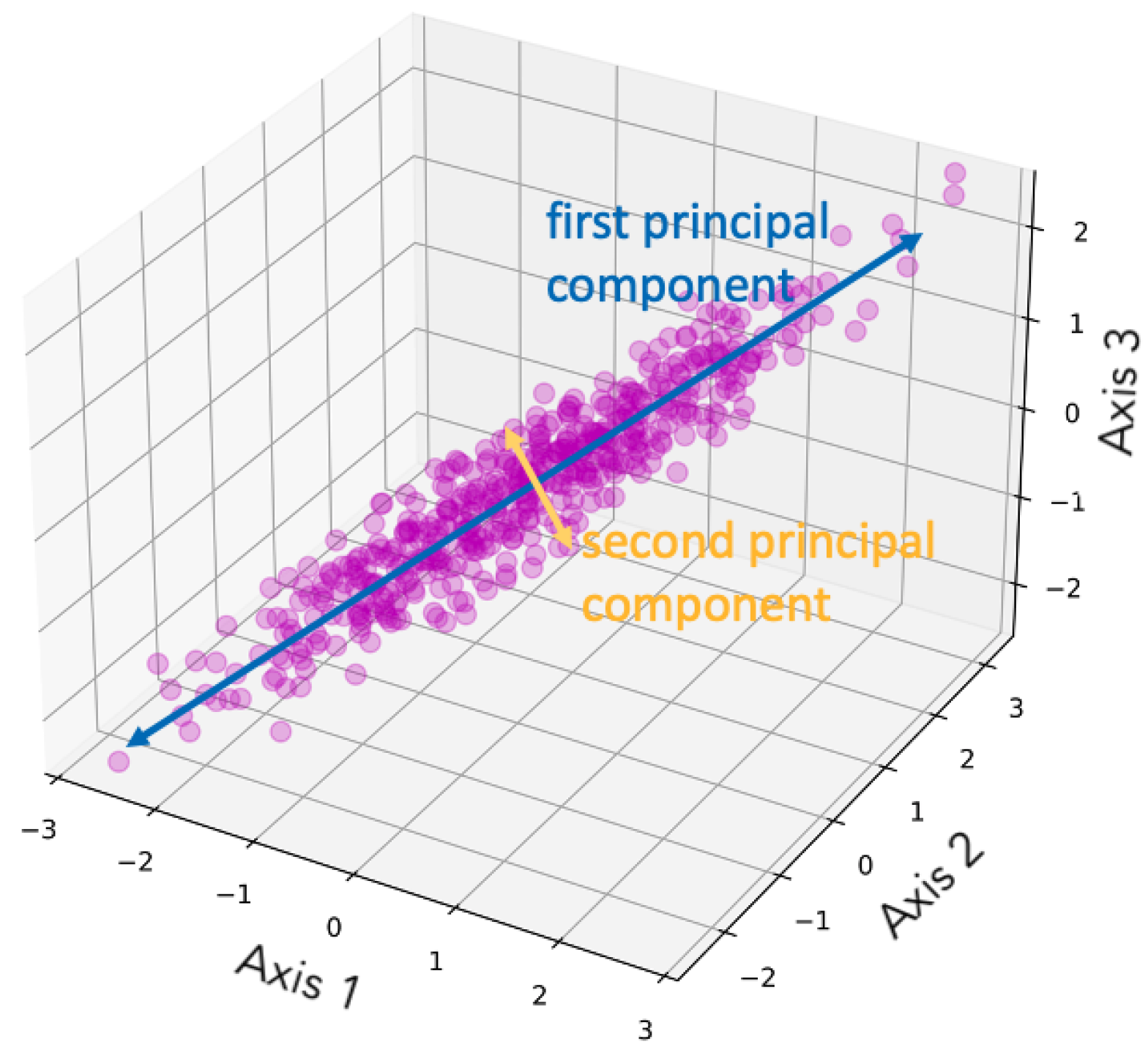
Figure 2.
Example of dimensionality reduction with PCA applied to images. Figure is taken from Çakir, U. and Buck, T. [21]. Licensed under CC BY 4.0.
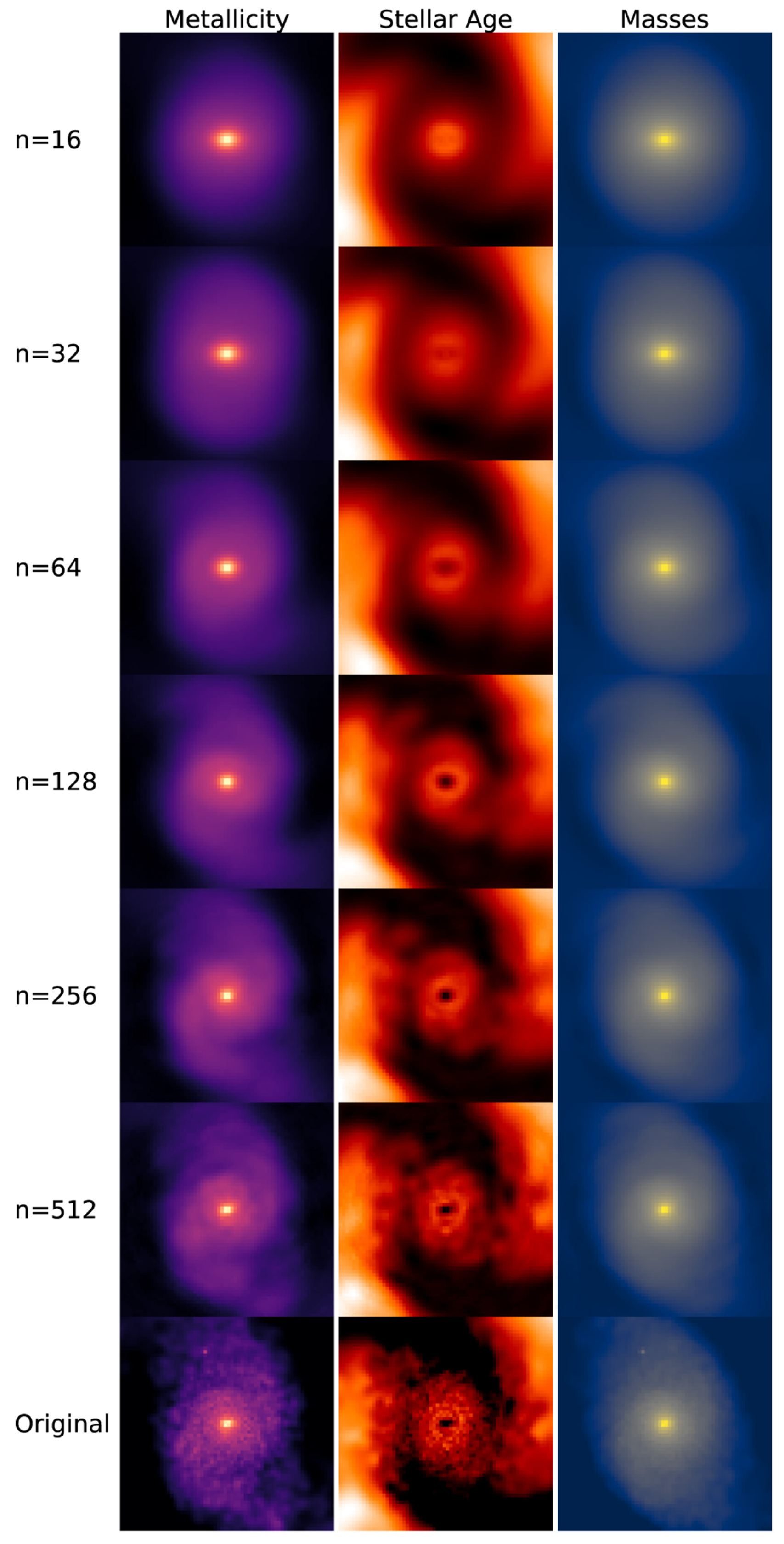
Figure 3.
Example of dimensionality reduction with (a) Isomap and (b) LLE (§2.3), showing how the two algorithms unroll a ‘Swiss roll’ manifold. Figure is taken from Fotopoulou [16]. Licensed under CC BY 4.0.
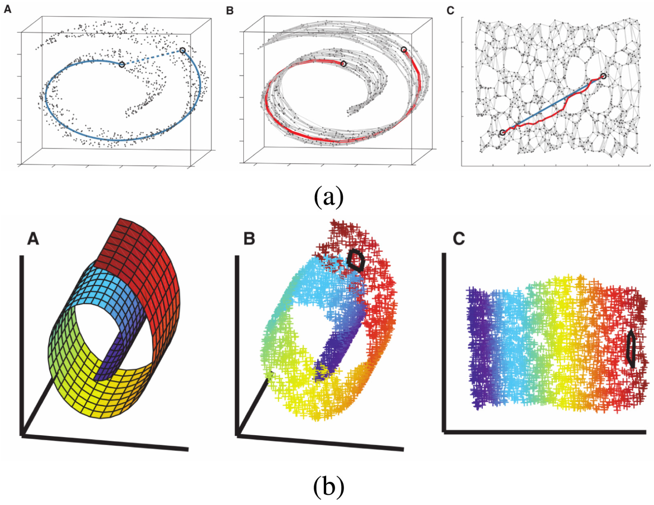
Figure 4.
Example of how t-SNE measures the affinity between two points, demonstrated using a three-dimensional data set, shown in (a). For example, the distance from any dot to the darkest black dot is computed, and the corresponding probability is determined using a Gaussian kernel, as shown in (b).
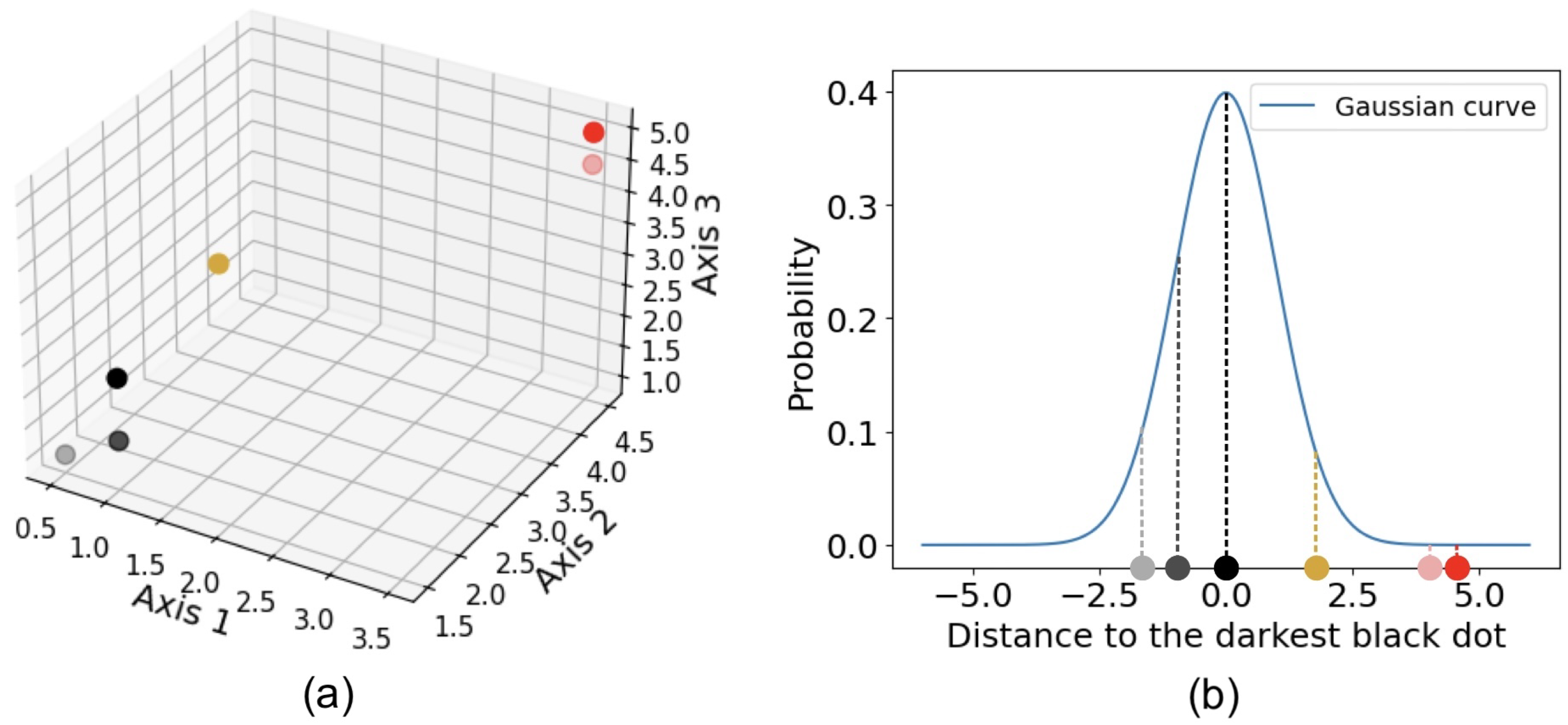
Figure 5.
Example of dimensionality reduction with t-SNE applied to spectral data. Figure is taken from Peruzzi, T. et al. [52]. Licensed under CC BY 4.0.
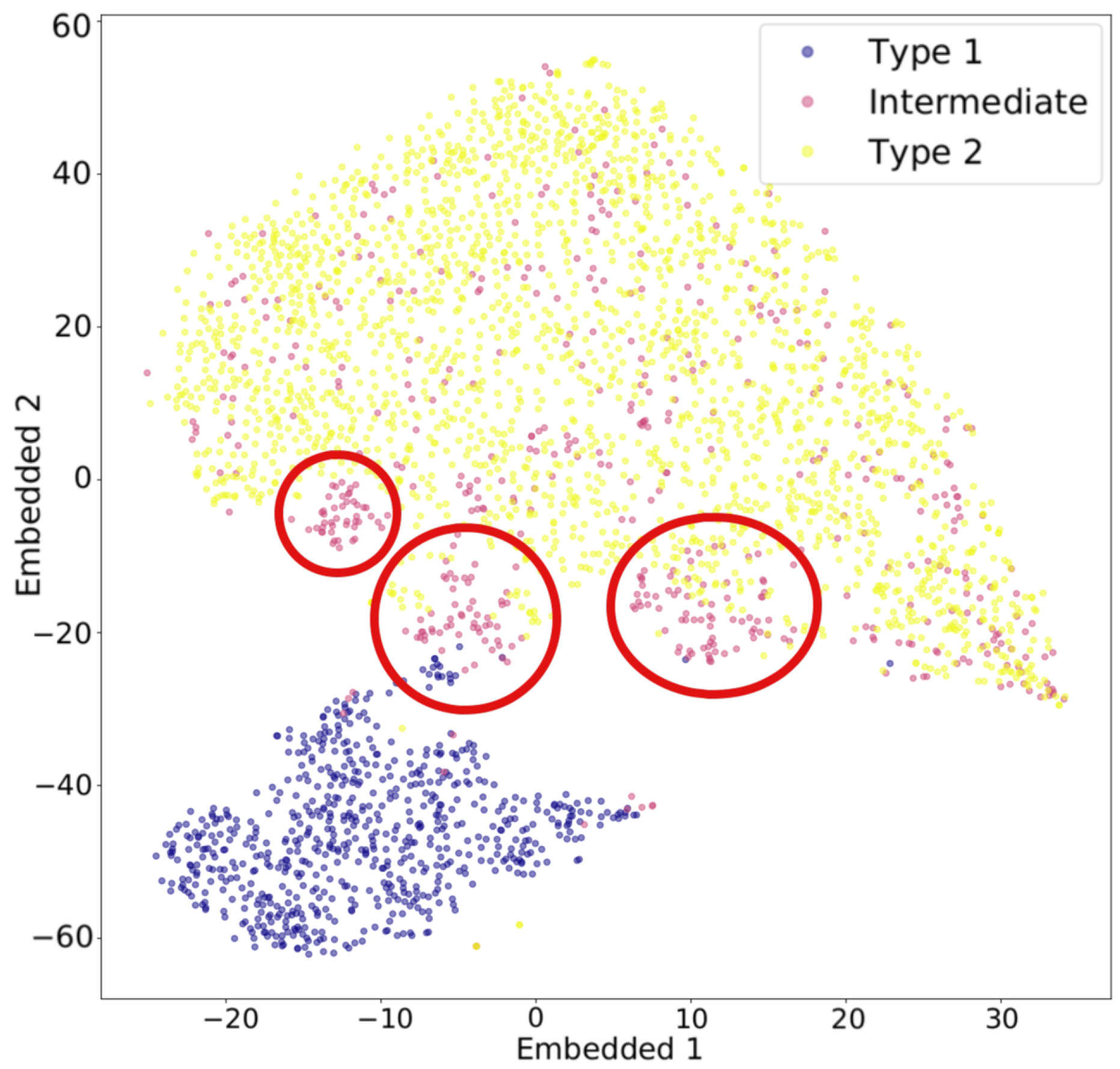
Figure 6.
Results of the dimensionality reduction algorithms, applied to the same five-dimensional data set. The algorithms include PCA, LLE, non-metric MDS, and t-SNE. The five-dimensional data set is clustered with DBSCAN before being reduced to two dimensions, where different colors represent different clusters, and the black dots represent the outliers. This figure illustrates how the clusters are distributed under different dimensionality reduction algorithms.
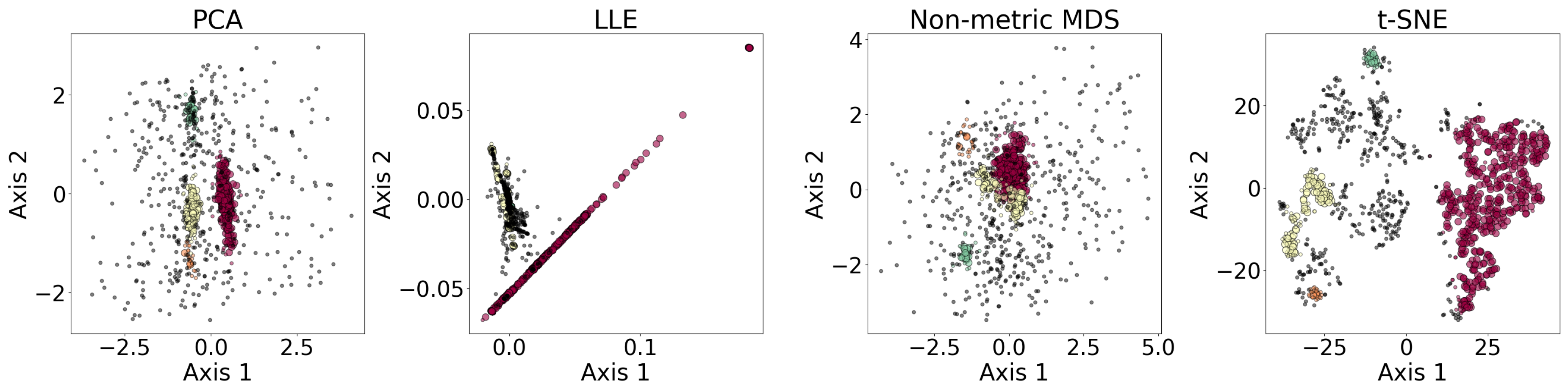
Figure 7.
Example of clustering with GMM, where two components are considered for clustering. The lines show the equi-probability contours of the model, making a contour plot of the sum of the two Gaussian functions. Figure generated using code adapted from the scikit-learn documentation: scikit-learn.org.
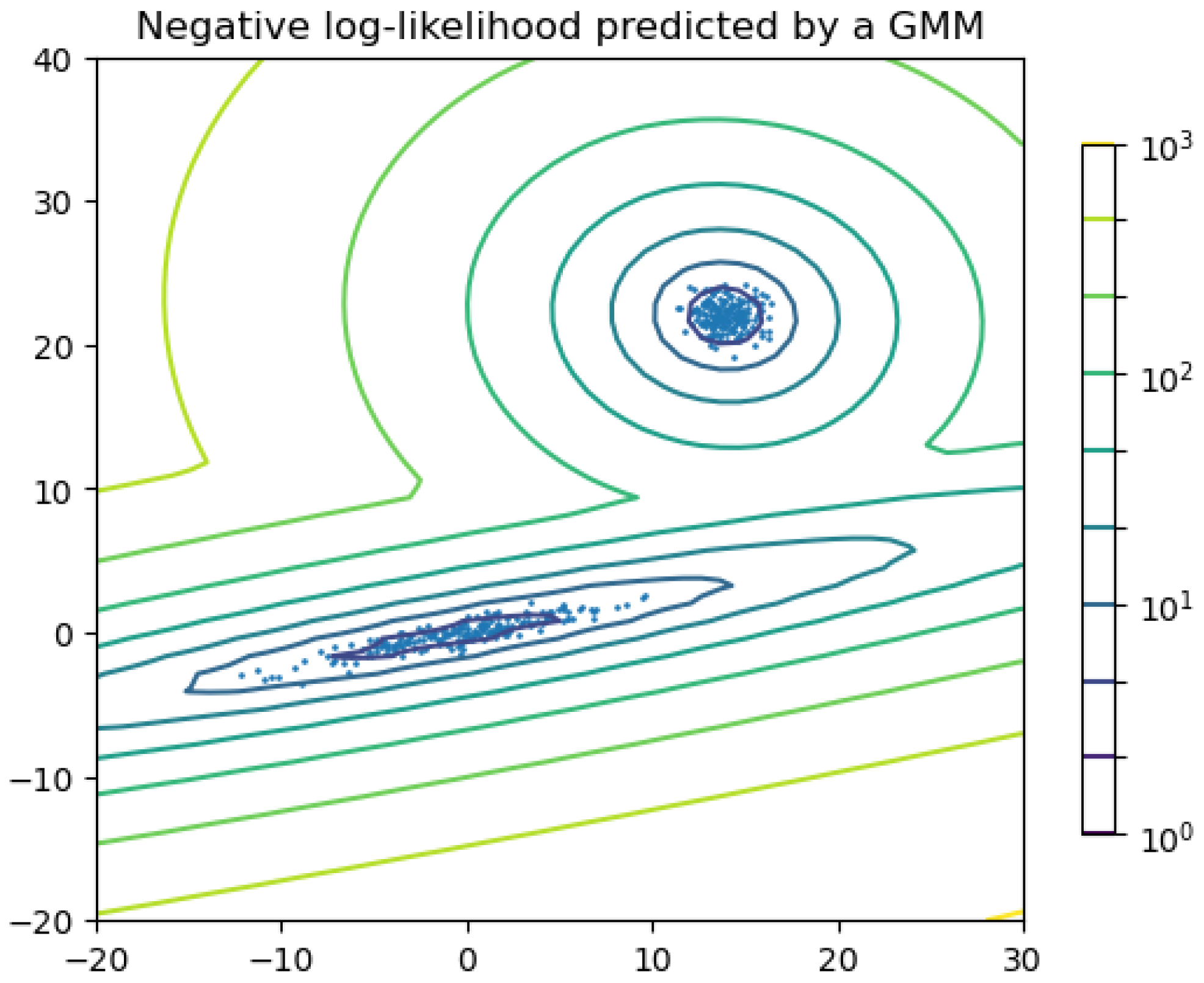
Figure 8.
Hierarchical clustering dendrogram for the bottom-up approach. The dashed line shows the level selected for clustering when 4 clusters are required, and the dotted line shows the level selected when 6 clusters are required.
Figure 8.
Hierarchical clustering dendrogram for the bottom-up approach. The dashed line shows the level selected for clustering when 4 clusters are required, and the dotted line shows the level selected when 6 clusters are required.
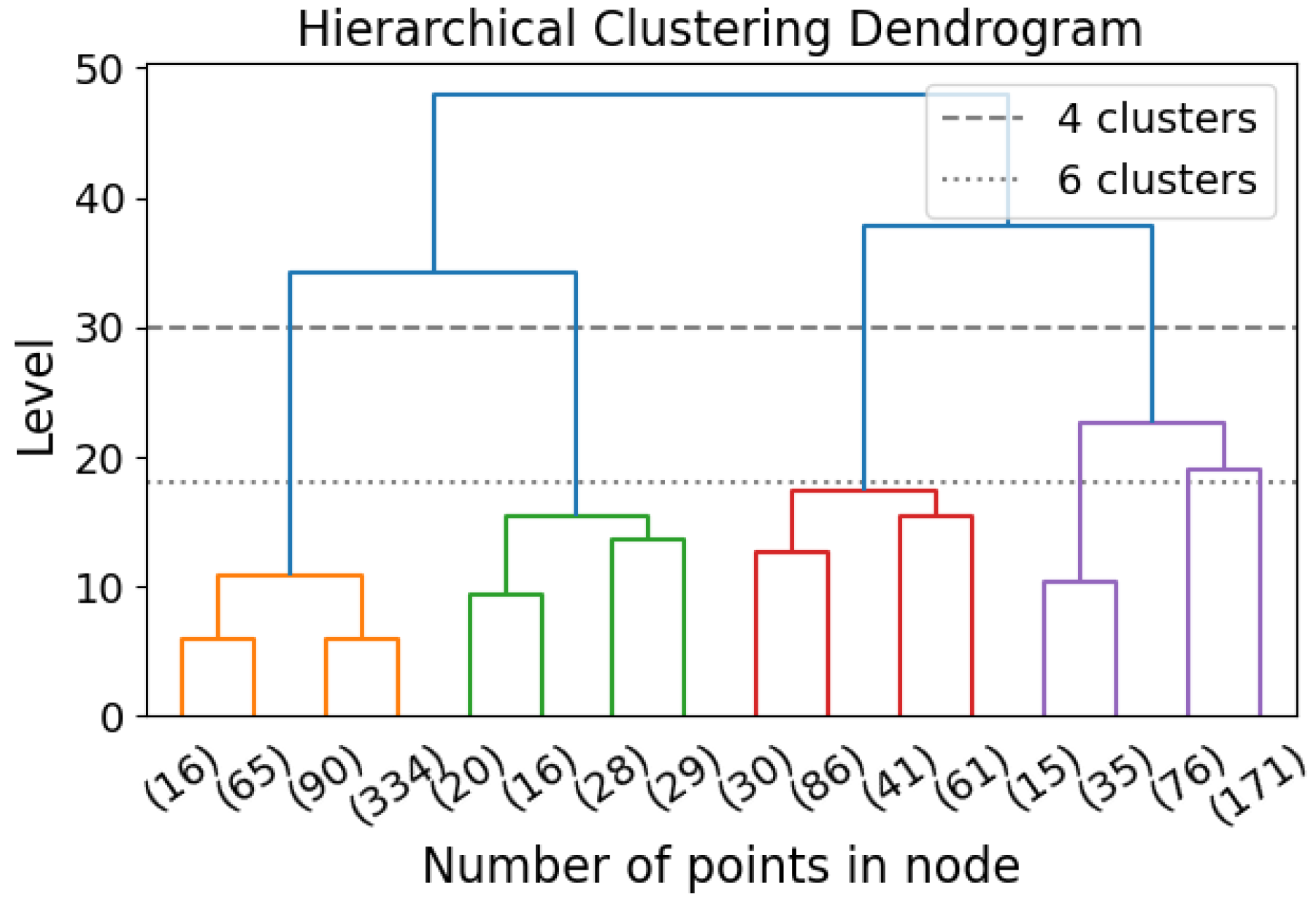
Figure 9.
Example of clustering with FCC applied to scattered data. The intensity of each data point reflects the probability of its membership in the cluster. Figure is taken from Colazo et al. [96]. Licensed under CC BY 4.0.
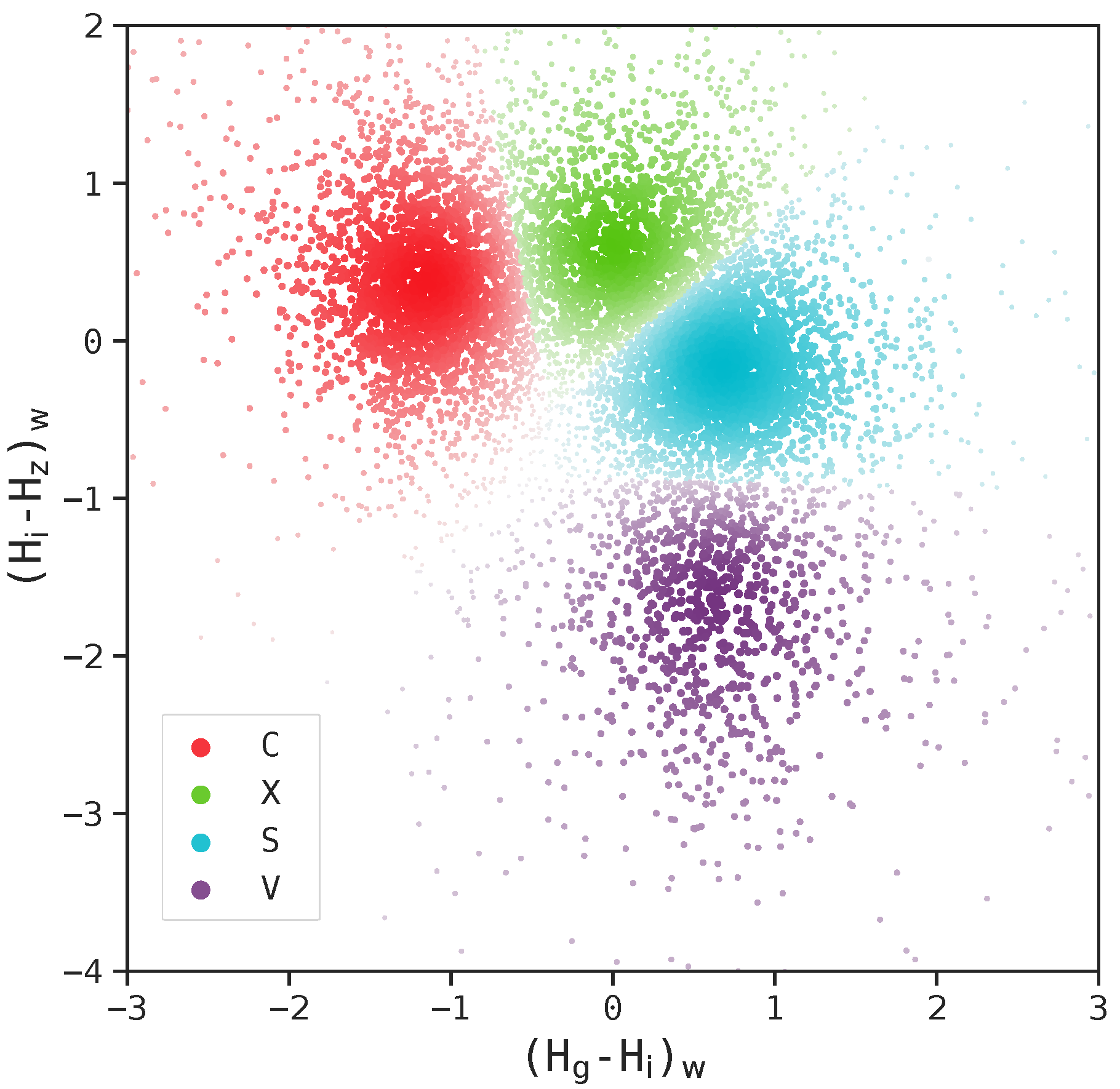
Figure 10.
The clustering algorithms are applied to the same five-dimensional data set, with the number of clusters set to four based on the BIC calculation. For algorithms that do not take the number of clusters as a hyperparameter, their hyperparameters were selected to yield four clusters. The algorithms include GMM, K-means, HC, DBSCAN, FCC, and SOM. The dataset is dimensionally reduced with PCA to a two-dimensional projection after the data set is clustered. The colors of the clusters are selected manually. When interpreting the results, note that PCA may not provide the best representation of the clusters; therefore, overlapping clusters or other irregularities do not necessarily indicate a failure of the algorithm. Among the six algorithms, GMM and DBSCAN yield similar results by recognizing outliers, while K-means and HC produce similar clusterings.
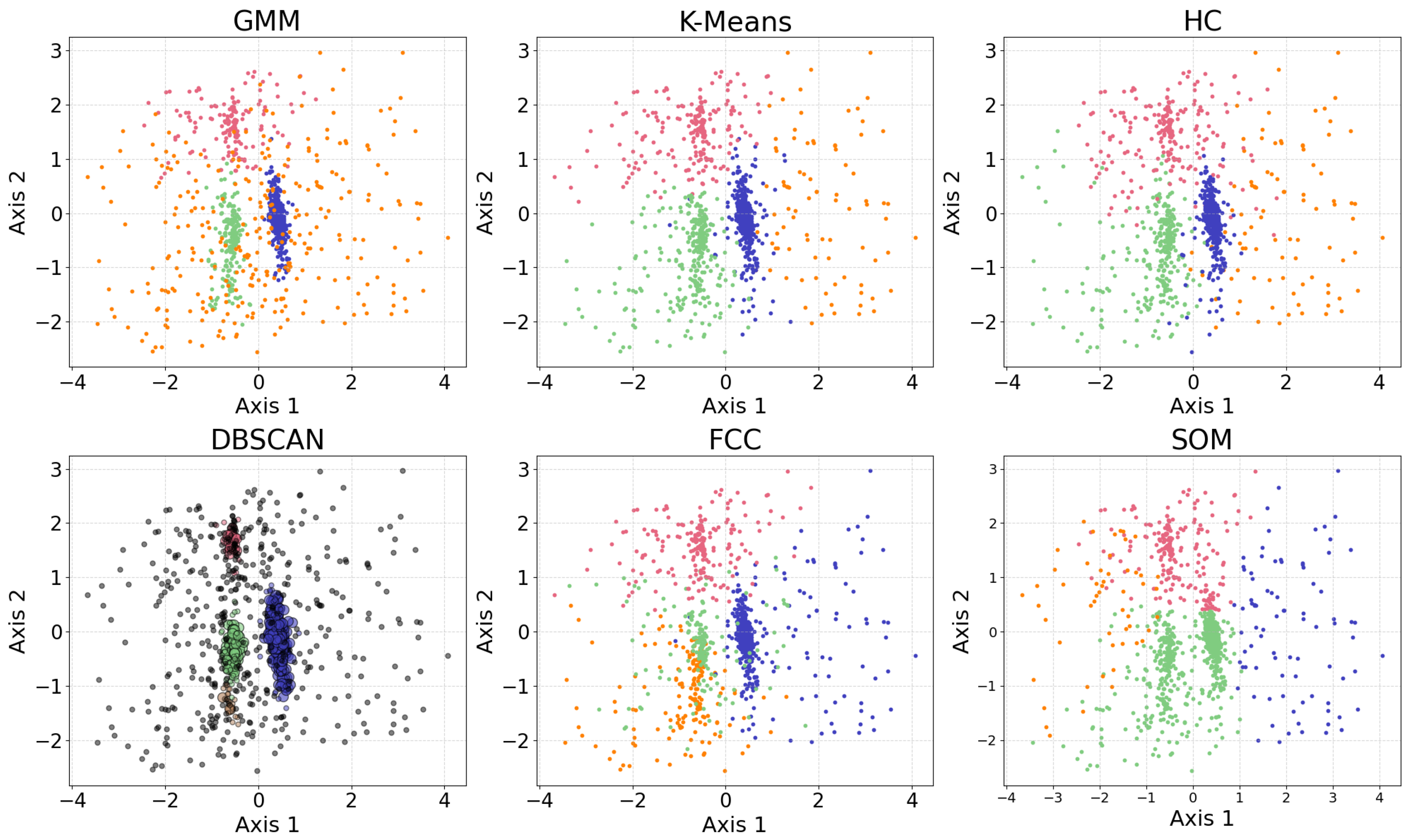
Figure 11.
Visualization of the SOM grid overlaid on the two-dimensional input data. The purple dots represent neuron weights, and the black lines connect neighboring neurons, illustrating how the SOM captures the underlying data topology.
Figure 11.
Visualization of the SOM grid overlaid on the two-dimensional input data. The purple dots represent neuron weights, and the black lines connect neighboring neurons, illustrating how the SOM captures the underlying data topology.
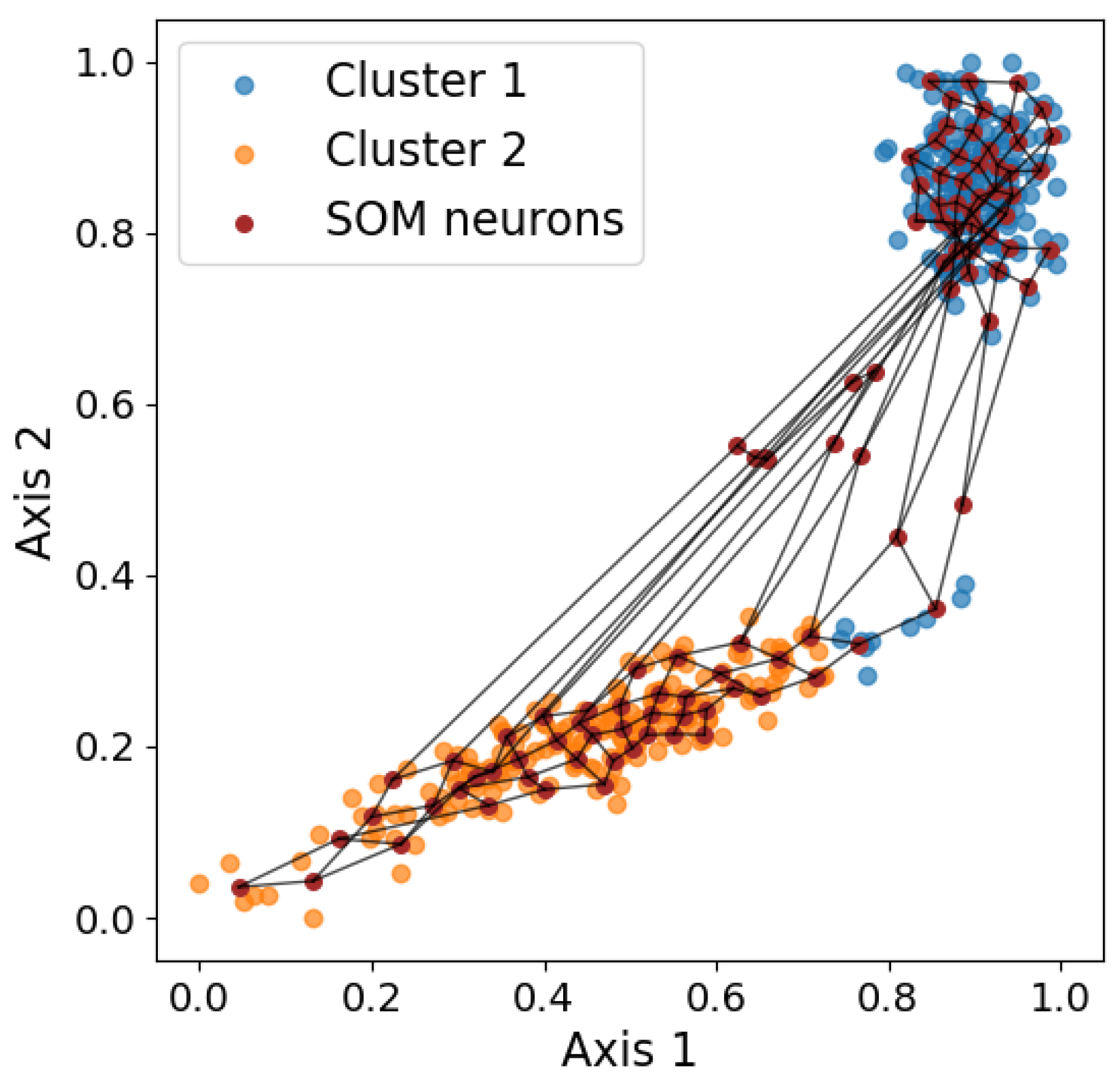
Figure 12.
Structure of AE, showing the input and output layers, encoder and decoder, and bottleneck. A shallow neural network has one or two hidden layers, while deep learning models have three or more. The figure is adapted from Fotopoulou [16], which was adapted from Kramer [114]. Licensed under CC BY 4.0.
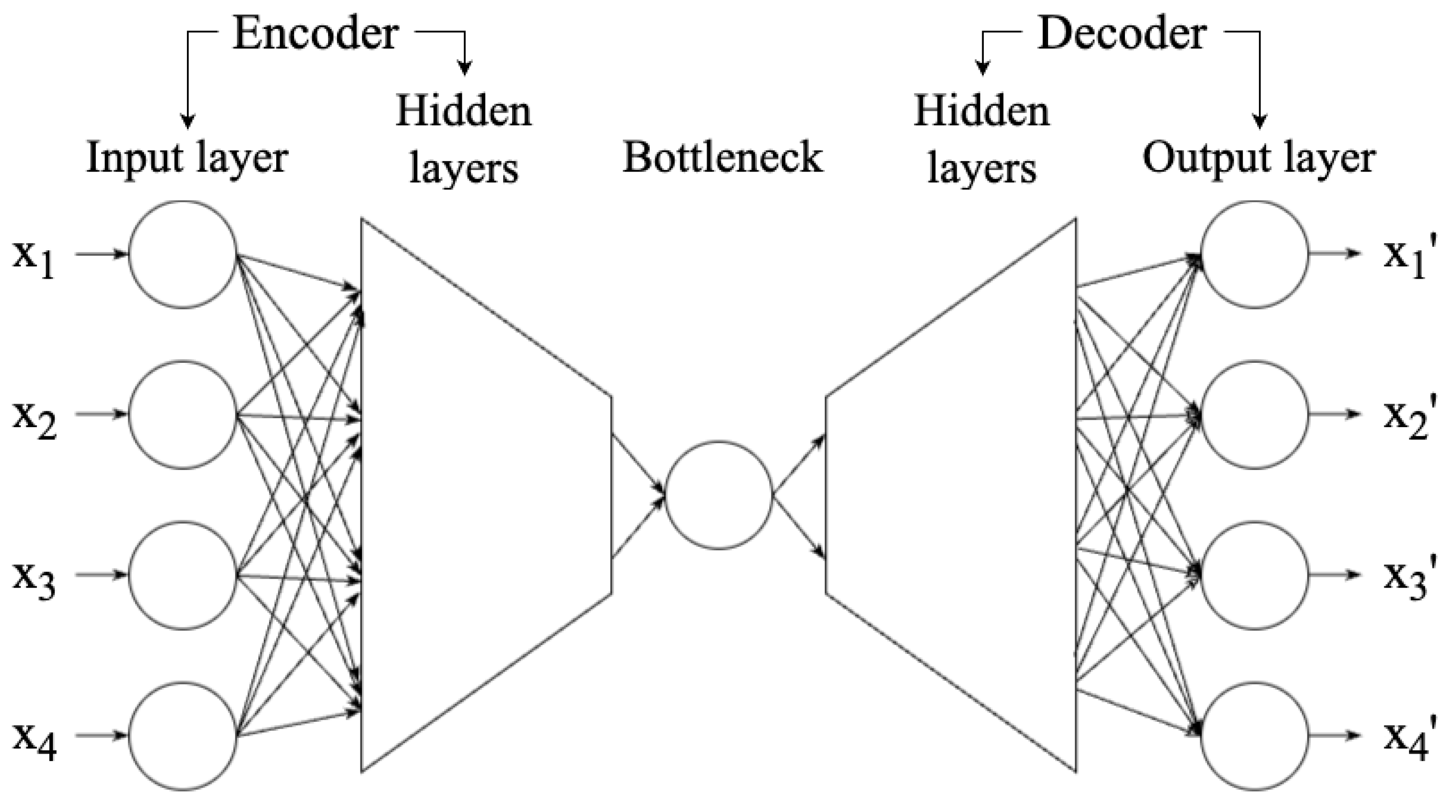
Figure 13.
Results of outlier detection using GMM, DBSCAN, SOM, and iForest, on the five-dimensional data set, then presented using PCA. The labeled inliers are the blue dots, and the labeled outliers are the black dots. The four anomaly detection algorithms are able to identify the three major clusters to some extent. Under PCA visualization, both GMM and SOM label a few points along the edge of the cluster as outliers, while DBSCAN and iForest consider half of the upper cluster as outliers. Again, PCA may not provide the best representation of the clusters, so irregularities do not necessarily indicate a failure of the algorithm.
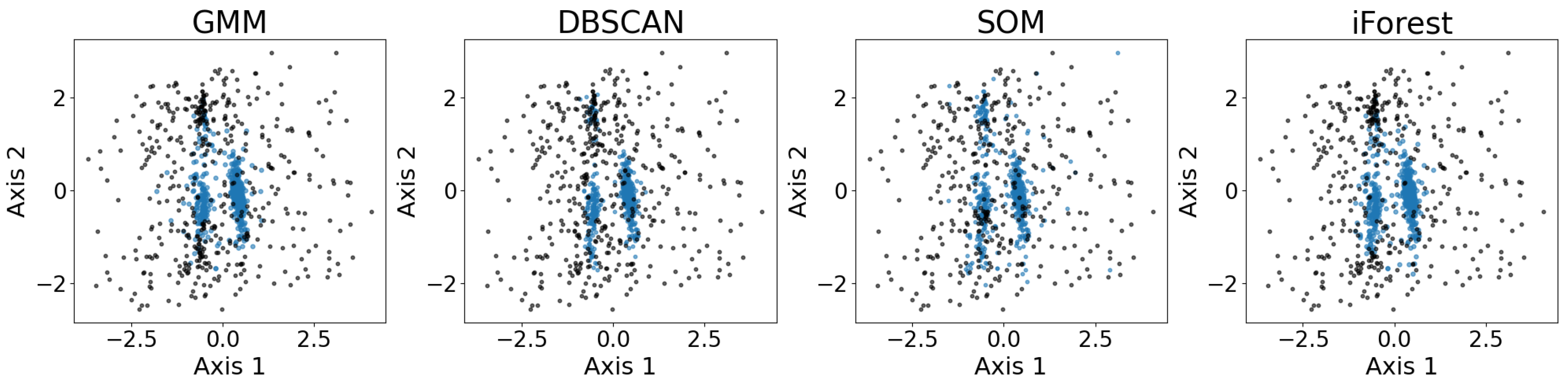

Table 1.
Result of a focused search, showing the number of refereed astronomy papers in ADS that applied each dimensionality reduction algorithms to different types of data from 2015 to 2025.
Table 1.
Result of a focused search, showing the number of refereed astronomy papers in ADS that applied each dimensionality reduction algorithms to different types of data from 2015 to 2025.
| PCA | MDS | Isomap | LLE | t-SNE | |
|---|---|---|---|---|---|
| Spectral data | 251 | 1 | 2 | 5 | 18 |
| Image | 106 | 0 | 1 | 0 | 7 |
| Catalogs | 35 | 0 | 1 | 5 | 14 |
| Photometry data | 46 | 0 | 0 | 2 | 7 |
| Light curves | 31 | 0 | 0 | 3 | 4 |
| Polarimetric data | 9 | 0 | 0 | 0 | 0 |
| Latent space | 3 | 0 | 1 | 0 | 0 |
Table 2.
Result of a focused search, showing the number of refereed astronomy papers in ADS that applied each clustering algorithms to different types of data from 2015 to 2025. The box corresponding to the most popular application of each algorithm is highlighted.
Table 2.
Result of a focused search, showing the number of refereed astronomy papers in ADS that applied each clustering algorithms to different types of data from 2015 to 2025. The box corresponding to the most popular application of each algorithm is highlighted.
| GMM | K-means | HC | DBSCAN | HDBSCAN | FCC | |
|---|---|---|---|---|---|---|
| Spectral data | 43 | 76 | 19 | 18 | 11 | 1 |
| Catalogs | 48 | 27 | 22 | 31 | 22 | 1 |
| Image | 36 | 70 | 13 | 13 | 2 | 3 |
| Photometry data | 51 | 14 | 8 | 14 | 26 | 1 |
| Bivariate data | 11 | 11 | 12 | 1 | 1 | 0 |
| Light curves | 10 | 9 | 3 | 3 | 3 | 0 |
| Polarimetric data | 2 | 7 | 0 | 0 | 0 | 0 |
| Latent space | 3 | 0 | 0 | 0 | 0 | 0 |
Disclaimer/Publisher’s Note: The statements, opinions and data contained in all publications are solely those of the individual author(s) and contributor(s) and not of MDPI and/or the editor(s). MDPI and/or the editor(s) disclaim responsibility for any injury to people or property resulting from any ideas, methods, instructions or products referred to in the content. |
© 2025 by the authors. Licensee MDPI, Basel, Switzerland. This article is an open access article distributed under the terms and conditions of the Creative Commons Attribution (CC BY) license (http://creativecommons.org/licenses/by/4.0/).
Copyright: This open access article is published under a Creative Commons CC BY 4.0 license, which permit the free download, distribution, and reuse, provided that the author and preprint are cited in any reuse.


