
Submitted:
09 July 2025
Posted:
10 July 2025
You are already at the latest version
Abstract
Investors study forecasting models for future stock values to make assertive decisions, as each trend movement offers different investment opportunities. The forecasting models described in this research are well suited to provide a realistic view of the future behaviour of stock prices. The autoregressive integrated moving average (ARIMA) model is one of the most relevant linear models for time series forecasting. Recurrent neural networks (RNN) are a class of neural networks that allow using previous outputs as inputs, while having hidden states and capturing the robust and non-linear relationships of the sequence. This paper proposes a hybrid methodology that takes advantage of the strengths of RNNs, linear and ARIMA models in value forecasting problems. Real datasets of Nvidia Corporation (NVDA) stock price on NASDAQ were used to analyse the forecasting accuracy of the proposed model. The main objective is to compare the performance of the combined model compared to each of them separately when it comes to stock price forecasting. By hybridising these models, the methodology is able to correctly predict the NVDA share price. The root mean square error (RMSE), mean absolute percentage error (MAPE) and mean absolute error (MAE) metrics were used to assess accuracy while coefficient of determination (R²) was used to measure goodness of fit.
Keywords:
ARIMA
; hybrid model
; LSTM
; NASDAQ stock market
; nvidia
; recurrent neural networks
; time series forecasting
1. Introduction
Stock price forecasting is an essential task in financial economics, enabling investors, financial analysts, and policymakers to make informed decisions. However, predicting stock prices remains a complex endeavor due to the inherent nonlinearity, volatility, and noise present in financial markets. Nvidia Corporation (NVDA), a leader in GPU and AI hardware technologies and one of the largest corporations by market capitalization [1], has shown significant growth and volatility, making it an ideal candidate for testing advanced forecasting techniques.
On the other hand, the last 50 years have seen significant advances in modelling and forecasting financial data, and the autoregressive integrated moving average (ARIMA) is one of the most widely used. One fundamental assumption for ARIMA models is that the future value and the historical values of the time series must satisfy a linear relationship. However, the main financial time series data contain a non-linear relationship due to their unstable structure and high volatility, which limits the scope of the application of the ARIMA model. [2]
Recently, several deep learning methods, especially artificial neural networks (ANNs), have obtained promising results in financial forecasting. A study by Li and Ma (2010) [3] found more than 40 researches on neural networks applied to economics and summarised that neural networks could discover non-linear relationships in input data, which made them compatible for modelling non-linear dynamic systems. Among all neural network models, the recurrent neural network (RNN) introduces the concept of time series in its design of architecture, which makes it more adaptable in the analysis of time series data.
In addition, the RNN network can detect the non-linear patterns in the sequence, and the ARIMA model can adjust the linear relationship in the series properly. By using a hybrid methodology, both linear and non-linear domains can be exploited and thus effectively predict the complex time series.
In summary, the proposed system consists of two basic methods that act synergistically. First, the RNN and ARIMA models are trained to predict the non-linear and linear parts of the data, respectively. Finally, the two predicted results are integrated to obtain the final predictions.
Following the same logic of variable weight analysis, a neural network (NN) system with twelve economic variables was used to analyse the significance of these variables in peso–dollar forecasting [4]. In the last decades, RNNs of the LSTM type have been widely used for forecasting sequential data [5,6,7,8]. The mechanism by which such networks store long- and short-term information makes them powerful when performing historical data forecasting. This type of RNN has been used for currency-pair forecasting, action trading on the New York Stock Exchange, recognition, environmental predictions, by comparing this method with other types of NNs and classical prediction methods [9,10,11,12]. Many of these comparisons and applications were used to formulate new hybrid models to improve the results of the predictions [13,14,15].
In this context, the results of a combination of classical forecasting methods [13], neural networks, and recurrent neural networks [16] have helped to clear the way for creating new approaches based on standard methods applied to foreign exchange rate and stock market forecasting [17]. Most of these approaches were proposed to find the model that can provide the best short-term prediction, which is the most challenging goal due to the inherently noisy and non-stationary behaviour of the data.
The aim of this paper is to provide valuable tools not only to demonstrate the accuracy of these models and use them for financial purposes, but also to show how these methods can be used to create hybrid models that may enhance time series forecasting. We begin this study by providing an overview of the two methods (ARIMA and RNN) to clarify how the algorithms work and how to optimise these models. Next, we define datasets used for training and validation, followed by exploratory analysis and pre-processing of the data. After that, we apply the LSTM (Long Short-Term Memory) which is a type of RNN. Then, we apply the ARIMA model to the residuals of the LSTM and optimal parameters were adjusted. For comparison, we hybridize an LSTM with a linear model as well. Training and validation of these methods are performed. Finally, we choose that method which provides the best short-term forecast, and the most accurate of these forecasting models is proposed.
2. Autoregressive Integrated Moving Average (ARIMA)
The ARIMA pioneered by Box and Jenkins is a flexible and powerful statistical method for time series forecasting [18]. The ARIMA model considers a time series as a random sequence and approximates the future values as a linear function of the past observations and white noise terms. Basically, the ARIMA consists of three components: 1. Non-seasonal differences for stationarity (I), 2. Auto-regressive model (AR), 3. Moving average model (MA) [19].
To understand the stationary difference order (I), the backward shift operator “B” is introduced, which causes the observation that it multiplies to be shifted backwards in time by 1 period. That is, for any time series R and any period t:
For any integer n, multiplying by B-to-the-nth-power has the effect of shifting an observation backwards by n periods.
Suppose denotes for the difference lag at time t which has a simple representation in terms of B. Let’s start the first-difference operation:
The above equation indicates that the differenced series r is obtained from the original series R by multiplying by a factor of . Therefore, in general the difference is given as:
The linear combination of AR process of order p (AR(P)) and MA model of order q (MA(q)) can be expressed as follows.
Where the constant are model orders, are model parameters, c is a constant, is the mean of the series, and is the random noise. Considering both and properties, can be written as:
Combining the above equation with Equation (5), the general form of the ARIMA model can be rewritten as:
Where represents the AR component, represents the MA component, d is the number of difference order and B is the backward shift operator such that if R is a time series.
3. Attention-Based Recurrent Neural Networks
Attention-based encoder-decoder networks were initially brought out in the field of computer vision and became prevalent in Natural Language Processing (NLP). In this document, the proposed ARNN follows the structure of a typical encoder-decoder network but with some modifications to perform time series prediction. [19]
Suppose T is the length of window size, for any time t, the n technical indicator series i.e. are the inputs for encoder, and m close price series i.e. are the exogenous inputs for decoder. Typically, given the future values of the target series (next hour’s close price) i.e. the ARNN model aims to learn a non-linear mapping between inputs (X and Z) and target series Y:
Where f is a non-linear mapping function that is a long-short term memory (LSTM). Each LSTM unit has a memory cell with the state at time t, which will be controlled by three sigmoid gates: forget gate , input gate and output gate . The LSTM unit is updated as follows:
Where is a concatenation of the previous hidden state and the current input . , and are parameters to learn. and ∘ are a logistic sigmoid function and an elementwise multiplication, respectively.
Encoder is essentially an LSTM that encodes the input sequences (technical indicators) into a feature representation. For time series prediction, given the input sequence with , the encoder can be applied to learn a mapping from to at time step t with
Where is the hidden state of the encoder, is the size of the hidden state and is a non-linear activation function in a recurrent unit. In this paper, we use stacked two-layer simple RNN as to capture the associations of technical indicators. The mathematical notation for the hidden state update can be formulated as:
Where is the weight matrix based on the previous hidden state and is the weight matrix based on the current input.
Decoder use another two-layer LSTM is used to decode the information from close price series i.e. with as:
Where is the hidden state of the decoder, is the size of the hidden state and is a non-linear activation function with the same structure as the in the encoder.
Attention mechanism express the input of the encoder by a context vector as the weighted sum of hidden states that corresponds to the output of the decoder where is the hidden state in the encoder, and is the attention coefficient of sequence obtained from the softmax function:
Where is called the alignment model, which evaluates the similarity between the input of encoder and the output of decoder. The dot product is used for the similarity function g in this paper. Given the weighted sum context vector , the output series of decoder can be computed as:
Where is the hidden state of the decoder, is the output of the decoder and function is chosen as elementwise multiplication in this paper. To predict target , we use a third LSTM-based RNN on the decoder’s output (s):
Where is one RNN unit, and b are parameters of dense layers that map the RNN neurons to the size of the target output.
4. Hybrid Approach
It has been argued that the hybridization of linear and nonlinear models performs better than individuals for time series forecasting [2]. Various types of combining methodologies have been proposed in the literature. Zhang [20] introduced an ARIMA-ANN model for time series forecasting and explained the advantage of combination via linear and non-linear domains. They claimed that the ARIMA model fitting contains only the linear component and the residuals contain only the nonlinear behavioral patterns that can be predicted accurately by the ANN model. Rout [21] implemented adaptive ARIMA models to predict the currency exchange rate finding that the combined models achieved better results. More recently, RNNs which can capture the sequence information were preferred than the simple neural networks to be used in the hybrid models for price predictions [22]. It was also emphasized [23] that the sequential order of combining RNN and ARIMA models impacted on the final predictions and running RNN before ARIMA model provided better accuracy. The same run-time sequence was adopted in this research.
5. RNN-ARIMA Model
In terms of modelling sequence, there are two possible ways to combine the RNN and ARIMA models. The first method is to use an ARIMA model to forecast the stock price and an RNN to predict the residual. The other method is to use RNN to predict the stock price and an ARIMA model to forecast the residual. This research adopted the second method as it has been proven suitable for financial data [21]. Figure 1 shows the high-level flowchart of the hybrid approach.
Figure 1.
High level block diagram of the proposed model.
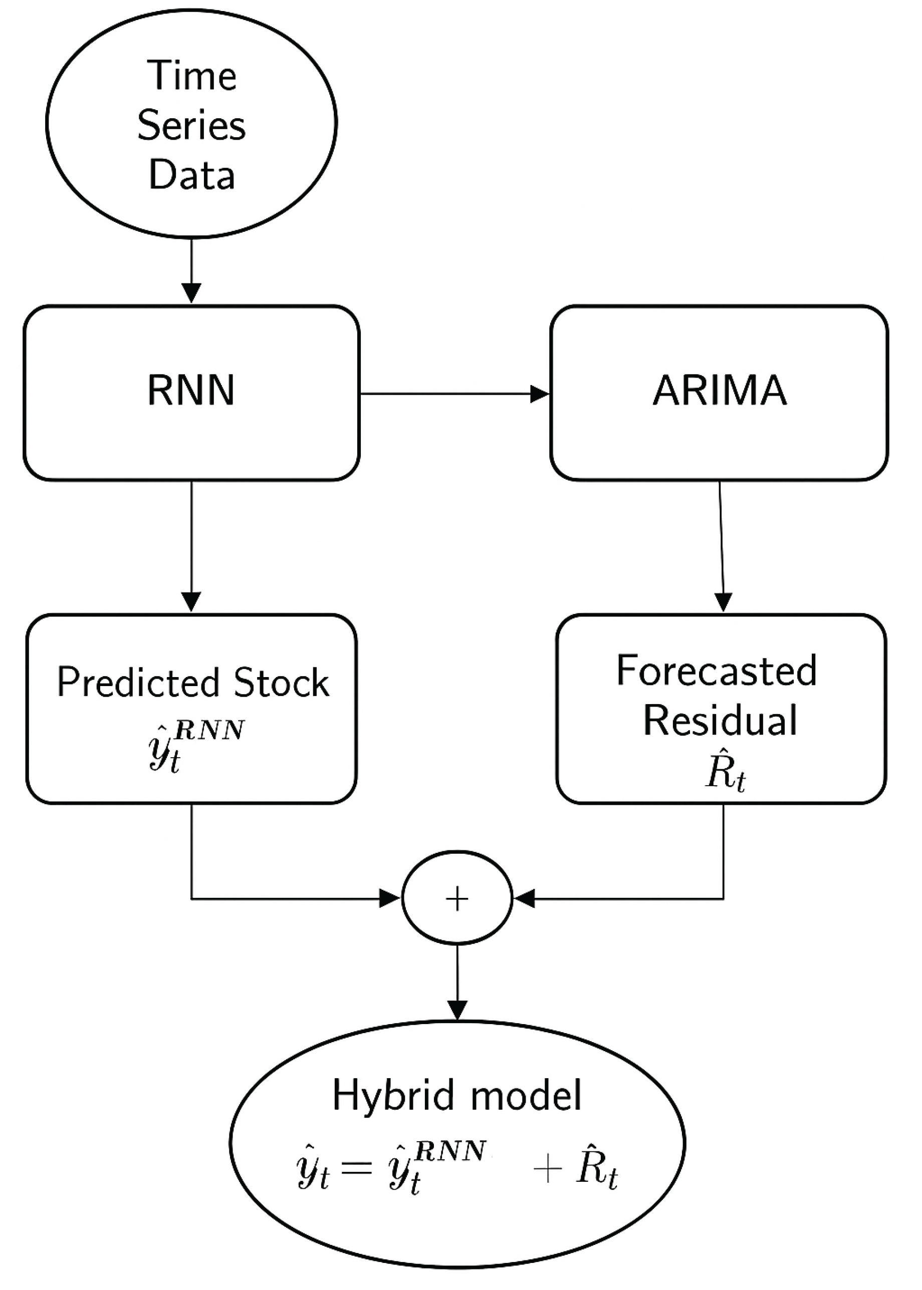
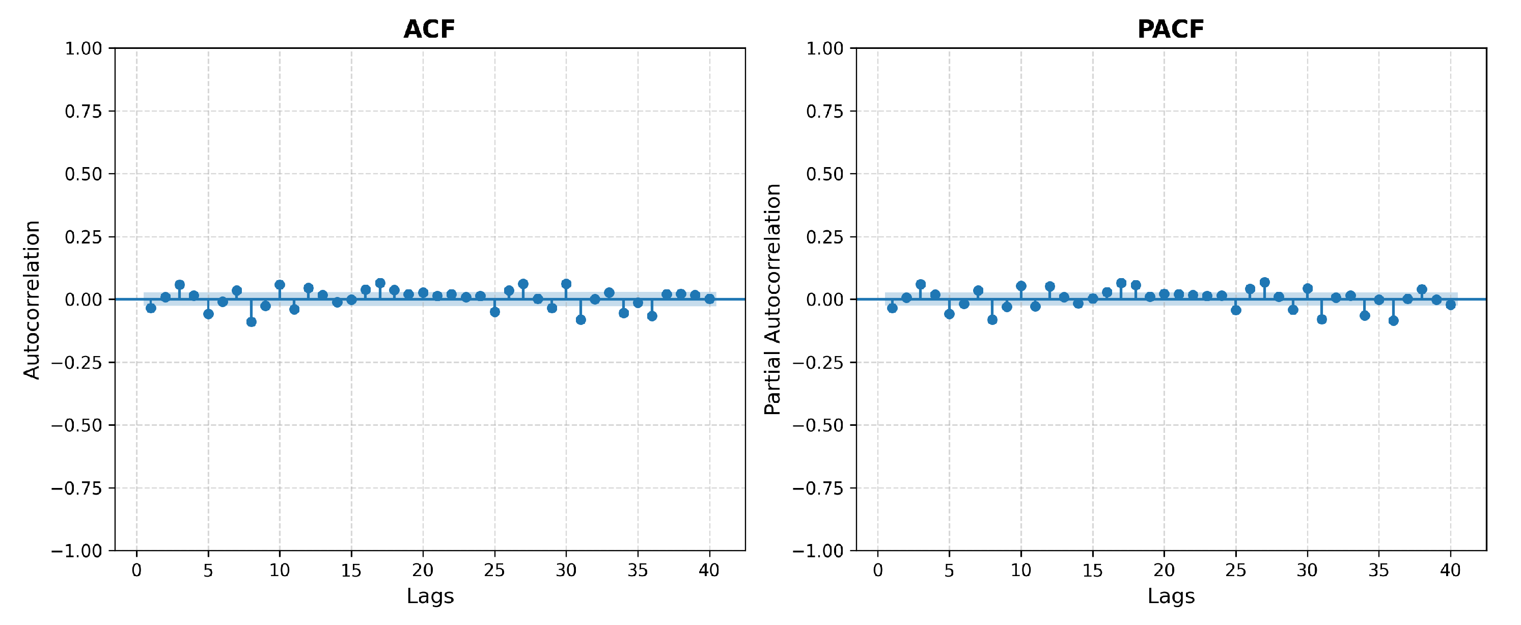
Figure 2.
Autocorrelation and Partial Autocorrelation Functions plots for NVDA Close price.
The RNN is firstly used to predict the stock price , then the residual can be calculated as the difference of prediction () and ground truth .
This residual series is modelled using an ARIMA model, and the final forecast () is computed by combining the prediction from RNN () and residual from ARIMA ().
6. Data Collection and Pre-Processing
The data in the experiment covers 6650 daily records of the adjusted stock close price from 1999-01-22 to 2025-06-30 collected from the Yahoo Finance API. Descriptive Statistics of NVIDIA stock closing price are shown in Table 1. Figure 3 shows the daily trend of the stock price of the obtained data since 2020. High volatility can be seen and an upright trend. To evaluate the performance meanwhile avoid overfitting the last 20% of samples are used for testing and the first 80% are the training set as shown in Table 2. At first, LSTM model was run. And after that, the hybrid models were applied: LSTM + ARIMA and LSTM + Linear regression. The residuals from the predictions obtained by the RNN model were used as input in the ARIMA and linear models. And finally, the three models were compared.
When using the machine learning methods, the original data are usually normalized before modelling to remove the scale effect. In this experiment, Min-Max-scale is conducted on the input data for the RNN model.
Where is the data after normalization, and , are the minimum and maximum data of the input (X). After modelling, the target output are anti-normalized.
Where is the predictive value after anti-normalization, is the predictions vector directly derived from the proposed model, and , are the minimum and maximum values of the target data (Y).
7. Performance Evaluation Criteria
Three evaluation metrics are used to assess the predictive accuracy: (1) the root-mean-squared-error (RMSE), (2) the mean-absolute-percentage-error (MAPE) and (3) the mean absolute error (MAE). The RMSE is defined as:
Where and are the prediction and ground truth at time t, and N is the number of test samples.
Compared to the RMSE, the MAPE eliminates the influence of the magnitude by using the percentage error, which can be calculated as:
On the other hand, the MAE is defined as follows:
The RMSE, MAPE and MAE are positive numbers, and the smaller (or closer to 0) the values, the higher the accuracy of the model.
8. Parameter Settings
For the RNN model, a grid search was conducted finding the following parameters to achieve the best accuracy on the validation set: number of units (50), dropout rate (0.1), batch size (16) and number of epochs (30).
The residual series obtained as the difference of the RNN predicted values and actual values, which is expected to account for only the linear and stationary part of the data. The best model was found using the function auto_ with the following parameters (p=5,d=0,q=2).
The model was structured and trained through the Google’s Colaboratory platform with GPU support in the Python3 programming language. The GPU model provided here is the Tesla K80 with pre-installed commonly used frameworks such as TensorFlow. And the hardware space is 2vCPU @ 2.2GHz, 13GB RAM, 33GB Free Space, GPU instance 350 GB.
9. Results and Discussion
Figure 2 shows the Autocorrelation Function (ACF) and Partial Autocorrelation Function (PACF) plots of the original NVDA stock closing price time series. Both plots exhibit significant autocorrelation at multiple lags, especially in the ACF, which displays a slow decay. This behavior confirms the presence of non-stationarity in the raw time series, typically associated with strong trend components and long-range dependencies. Recognizing this, a Long Short-Term Memory (LSTM) neural network was first applied to model the nonlinear temporal patterns. The remaining residuals, representing the components not captured by the LSTM, were then further refined using an model to improve forecasting performance. This two-step hybrid strategy leverages the strength of LSTM in capturing complex patterns and ’s effectiveness in modeling linear dependencies in the residual structure.
Table 3 demonstrates the accuracy metrics of the proposed model (RNN+) in comparison to the RNN and RNN-linear models.
From Table 3, clearly the RNN alone has lower MAE and MAPE values compared to RNN- and RNN-linear, which confirms the goodness of applying Neural Networks models in financial time series prediction. Nevertheless, the hybrid approach combining RNN and linear regression has outperformed the RNN with a better goodness of fit (R²=0.9957) and the least RMSE (2.74). Fig. 4 shows the predictions of the three models to the test set. Linear regression helps reduce the gap between the predictions from RNN and the actual values when they are mixed, hence improving the model performance.
10. Conclusions
This research proposes a hybrid approach consisting of RNN and ARIMA/linear model for predicting the stock close price of NVIDIA corporation in the NASDAQ stock exchange. The experimental results in Table 3 confirms that the integrated system linear-RNN (R²=99.58% and RMSE=2.74) performs slightly better than single Recurrent Neural Networks (R²=99.49% and RMSE=2.99) or RNN-ARIMA (R²=99.47% and RMSE=3.05) when applying to the test data from 2020 to mid-2025 while the RNN alone has a better MAE (1.61) and MAPE (3.36%). Although the proposed system achieved good accuracy, there are some limitations of the model. At first, the model did not consider all the variables involved in the process such as the market’s emotions and other relevant economic variables. This approach should be taken into account in future researches. Furthermore, this kind of models does not have a satisfactory performance when dealing with limited amount of data.
References
- CompaniesMarketCap. Largest Companies by Market Cap. https://companiesmarketcap.com/, n.d. Accessed: 2025-05-16.
- Zeng, Z.; Khushi, M. Wavelet Denoising and Attention-based RNN-ARIMA Model to Predict Forex Price. Review of Scientific Instruments 2020, abs/2008.06841, 1236–1239.
- Li, Y.; Ma, W. Applications of artificial neural networks in financial economics: a survey. International symposium on computational intelligence and design 2010, 1, 211–214.
- Zapata Garrido, L.A.; Díaz Mojica, H.F. Predicción del tipo de cambio peso-dólar utilizando Redes Neuronales Artificiales (rna). Pensamiento & Gestión 2008, 1, 29–42.
- Van Houdt, G.; Mosquera, C.; Nápoles, G. A review on the long short-term memory model. Artif. Intell. Rev. 2020, 53, 5929–5955. [CrossRef]
- Yıldırım, D.C.; Toroslu, I.H.; Fiore, U. Forecasting directional movement of Forex data using LSTM with technical and macroeconomic indicators. Financial Innovation 2021, 7, 1–36.
- Zhang, C.; Fang, J. Application research of several LSTM variants in power quality time series data prediction. In Proceedings of the Proceedings of the 2nd International Conference on Artificial Intelligence and Pattern Recognition, 2019, pp. 171–175.
- Choi, J.Y.; Lee, B. Combining LSTM network ensemble via adaptive weighting for improved time series forecasting. Mathematical problems in engineering 2018, 2018. [CrossRef]
- Babu, A.; Reddy, S. Exchange rate forecasting using ARIMA. Neural Network and Fuzzy Neuron, Journal of Stock & Forex Trading 2015, 4, 01–05.
- Adebiyi, A.A.; Adewumi, A.O.; Ayo, C.K. Comparison of ARIMA and artificial neural networks models for stock price prediction. Journal of Applied Mathematics 2014, 2014.
- Li, M.; Ji, S.; Liu, G. Forecasting of Chinese E-commerce sales: an empirical comparison of ARIMA, nonlinear autoregressive neural network, and a combined ARIMA-NARNN model. Mathematical Problems in Engineering 2018, 2018.
- Son, H.; Kim, C. A deep learning approach to forecasting monthly demand for residential–sector electricity. Sustainability 2020, 12, 3103.
- Wang, J.J.; Wang, J.Z.; Zhang, Z.G.; Guo, S.P. Stock index forecasting based on a hybrid model. Omega 2012, 40, 758–766. [CrossRef]
- Islam, M.S.; Hossain, E. Foreign exchange currency rate prediction using a GRU-LSTM Hybrid Network. Soft Computing Letters 2020, p. 100009.
- Musa, Y.; Joshua, S. Analysis of ARIMA-artificial neural network hybrid model in forecasting of stock market returns. Asian Journal of Probability and Statistics 2020, pp. 42–53.
- Qiu, Y.; Yang, H.Y.; Lu, S.; Chen, W. A novel hybrid model based on recurrent neural networks for stock market timing. Soft Computing 2020, pp. 1–18.
- Hu, Z.; Zhao, Y.; Khushi, M. A survey of forex and stock price prediction using deep learning. Applied System Innovation 2021, 4, 9.
- Asteriou, D.; Hall, S., ARIMA Models and the Box-Jenkins Methodology. In Applied Econometrics; Bloomsbury Publishing, 2016; pp. 275–296. [CrossRef]
- Zeng, Z.; Khushi, M. Wavelet Denoising and Attention-based RNN-ARIMA Model to Predict Forex Price. In Proceedings of the 2020 International Joint Conference on Neural Networks (IJCNN). IEEE, 2020, pp. 1–7.
- Zhang, G.P. Time series forecasting using a hybrid ARIMA and neural network model. Neurocomputing 2003, 50, 159–175.
- Rout, M.; Majhi, B.; Majhi, R.; Panda, G. Forecasting of currency exchange rates using an adaptive ARMA model with differential evolution based training. Journal of King Saud University-Computer and Information Sciences 2014, 26, 7–18.
- Rather, A.M.; Agarwal, A.; Sastry, V. Recurrent neural network and a hybrid model for prediction of stock returns. Expert Systems with Applications 2015, 42, 3234–3241.
- Weerathunga, H.; Silva, A. DRNN-ARIMA Approach to Short-term Trend Forecasting in Forex Market. In Proceedings of the 2018 18th International Conference on Advances in ICT for Emerging Regions (ICTer). IEEE, 2018, pp. 287–293. [CrossRef]
Figure 3.
Daily closing price series (NVDA) from 2020 to mid-2025.
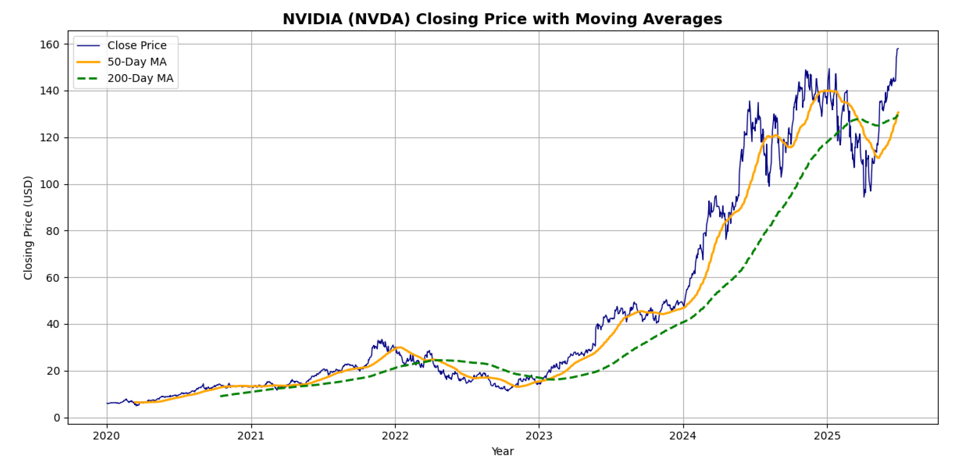
Figure 4.
The effect of the LSTM + /Linear model.
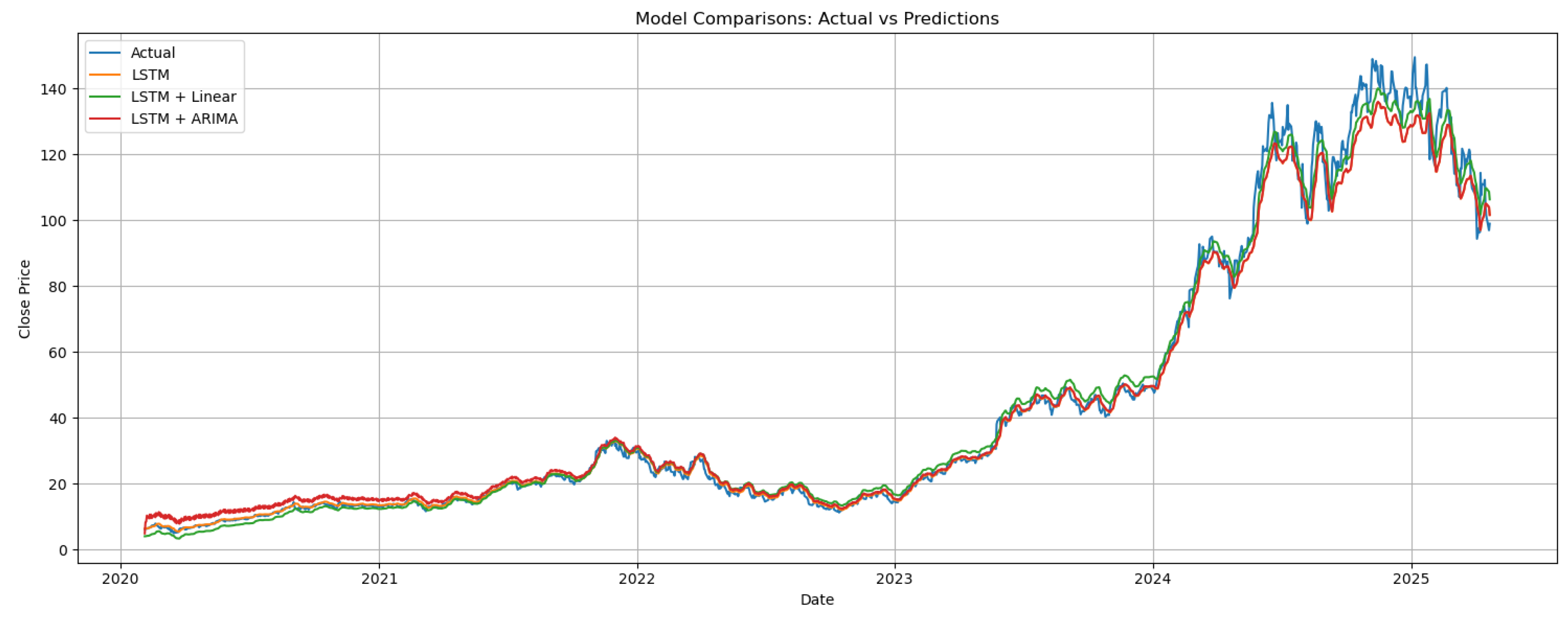

Table 1.
Descriptive statistics of NVIDIA stock closing price.
| Statistic | Value |
|---|---|
| Mean | 9.52 |
| Standard Deviation | 25.39 |
| Minimum | 0.03 |
| 25th Percentile (Q1) | 0.28 |
| Median (Q2) | 0.47 |
| 75th Percentile (Q3) | 4.82 |
| Maximum | 149.43 |
| Sample size | 6650 |
Table 2.
Sample composition in the dataset.
| Train | Test |
|---|---|
| 1999-01-22 to 2020-03-13 | 2020-03-16 to 2025-06-30 |
Table 3.
Experimental Results for closing Stock Price estimation.
| MODELS | MAE | RMSE | MAPE(%) | R² |
|---|---|---|---|---|
| RNN | 1.61 | 2.99 | 3.36 | 0.9949 |
| RNN + Linear | 1.65 | 2.73 | 4.69 | 0.9958 |
| RNN + | 1.88 | 3.06 | 6.12 | 0.9947 |
Disclaimer/Publisher’s Note: The statements, opinions and data contained in all publications are solely those of the individual author(s) and contributor(s) and not of MDPI and/or the editor(s). MDPI and/or the editor(s) disclaim responsibility for any injury to people or property resulting from any ideas, methods, instructions or products referred to in the content. |
© 2025 by the authors. Licensee MDPI, Basel, Switzerland. This article is an open access article distributed under the terms and conditions of the Creative Commons Attribution (CC BY) license (http://creativecommons.org/licenses/by/4.0/).
Copyright: This open access article is published under a Creative Commons CC BY 4.0 license, which permit the free download, distribution, and reuse, provided that the author and preprint are cited in any reuse.


