
Submitted:
05 July 2025
Posted:
07 July 2025
Read the latest preprint version here
Abstract
Utilizing several methods, this note shows that, in any collaboration network analysis, paper exclusion not only creates a loss of information, but can lead to incorrect interpretation of network structure because interpretation of vertex degree in the authors only graph is not well defined. Because the bipartite authors with papers graph is the actual social network, metric dimension is used to show that the relative distance structure of the bipartite graph is often defined by the structure of the papers, not that of the authors. Due to the NP-hard nature of metric dimension, methods that increase computational efficiency for the bipartite authors and papers graph are explored. With a departmental collaboration focus, public data for 245 professors from mathematics, physics and biology departments of three U.S. public universities is analyzed with network structure compared using metric dimension. By discipline, an average graph is defined with average graphs constructed from the collected data for the authors only structure, for the bipartite authors with papers structure and for papers only. Social analysis of the collected data shows that a 27\% change in the total number of hubs, along with identifying different professors as hubs, when the authors only graphs are compared to bipartite graphs reiterating the need for paper inclusion in any collaboration study.
Keywords:
collaboration network
; network evolution
; metric dimension
; Durfee square
; Durfee rank
; average graph
MSC: Primary 05C82; Secondary 05C12
1. Introduction
Most collaboration network studies examine the authors only structure although it is recognized that some information is lost when papers are excluded. This study shows that excluding papers can lead to misinterpretation of various aspects of the collaboration network structure, possibly making accurate modeling of the network evolution impossible.
Utilizing graphs as sociograms, with a focus on the departmental collaboration of 245 professors, data was collected for three STEM departments in three U.S. public universities where the average department size is similar to Zachary’s karate club mentioned in several social network papers [25]. To provide anonymity concerning the selected universities, the concept of an average graph is introduced with data analysis given for both graphs based on the collected data and the constructed average graphs. Used to compare the change in relative distance structure when papers are added to the authors only structure, metric dimension analysis reflects that the authors only structure does not necessarily preserve the relative distance structure of the actual collaboration network. For any bipartite graph G and utilizing G’s distance matrix (DM), DM block resolving provides an accurate but more efficient method for finding the metric dimension of G, . Denote the bipartite authors and papers graph with , the authors only graph by and the papers only graph as . Let be the DM block with both rows and columns indexed by author vertices and be the square block indexed by paper vertices . Proposition 9.1 shows that DM block resolving can be utilized to find and . Theorem 9.7 states that given only three DM blocks need to be resolved in order to find . Propositions 9.8 and 9.9 provide more efficient methods for determining given certain conditions such as Durfee rank of a graph comparison. This note appears to be the only social network analysis utilizing metric dimension to compare related social network structures, and the only one utilizing degree diagrams and the related Durfee rank of a graph.
In this study’s nine departments, an average of 50% of the faculty performed departmental collaboration between 2019 and 2023. Six of the nine department chairs did departmental collaboration with three of the six acting as collaboration hubs. In comparing the to the bipartite , the represents the actual social network, not the . Although there is an interpretation difference in large vertex degree in a compared to that of a , based on collaboration hubs, a comparison of the to the results in a 27% increase in the number of hubs, plus different authors are identified as the hubs. The large degree interpretation of the is also not well defined. This emphasizes the importance of paper inclusion and gives foundation for Conjecture 6.1 stating that accurately determining social network evolution models requires paper inclusion.
Although the use of graphs in studying networks preceded their paper, Harary and Norman’s 1953 article that connected graph theory to social network analysis [13] got serious attention. Price’s 1965 article [29] discusses the network structure of scientific papers based on the papers’ references. Another important social network study was conducted by Milgram in 1967 [23] where randomly selected individuals were asked to forward a letter to a stock broker in Boston. In 2001 Newman [24] utilized large scientific paper databases to study the collaboration structure of scientific research. Often used to compare networks, metric dimension was published independently by Slater in 1975 [32] and by Harary and Melter in 1976 [14]. Metric dimension was originally shown to be NP-complete in [6] but has been more recently shown to be NP-hard [15]. The metric dimension of complete bipartite graphs is given in [8] while [4] discusses for regular bipartite graphs. No exact method has been found for finding the metric dimension covering all bipartite graphs.
Because this note is written for a variety of possible readers, explanations are kept as simple as possible although basic graph theory knowledge is assumed. Section 2 provides graph theory notation and other possibly unfamiliar concepts important to this note. That section concludes with social network concepts and some results of other social network studies. Section 3 gives the data collection methods for this study. Vertex projection graphs based on the bipartite authors with papers graph are discussed in Section 4, while Section 5 discusses the structural specifics of the bipartite authors and papers graph. The social analysis in Section 6 interprets the data collected on departmental collaboration with respect to department chairs who act as hubs.
Since this study takes a close view of mathematics, physics and biology departments, the data analysis presentation focuses on concealment of which universities were used via average graph construction. The nine average graphs given in Section 7 are accompanied by brief discussions. The use of the degree diagram and the Durfee square with its rank as an analysis tool for bipartite graphs is discussed in Section 8. Section 9 covers the metric dimension analysis of the average graphs and methods for determining the metric dimension for the authors and papers bipartite graph. A focus on future work concludes this paper in Section 10 where the challenges presented by paper inclusion in collaboration studies utilizing large databases is briefly discussed.
2. Background Information
Whether this note’s readers are sociologists, statistical physicists or mathematicians, this note assumes basic graph theory familiarity as found in [9]. Utilized in many social analysis studies, a sociogram is a graph where vertices reflect people and/or social groups with edges representing vertex relationships. Graphs constructed from the collected data are referred to here as data derived graphs.
The Pigeonhole Principle states that given more pigeons than pigeonholes for the pigeons, and assuming that all of the pigeons find a pigeonhole, then at least one pigeonhole contains more than one pigeon.
2.1. Graph Theory Notation
A proper subset A of set X is denoted by with set cardinality given by and element x inclusion in X by . Graph G has vertex set with cardinality , or simply n, called G’s order. Edge set has cardinality , or m, and is G’s size. A vertex v in a specific graph G is . All G in this note are simple so multiple edges and loops are excluded. Graph G isomorphic to graph H is denoted with . The diameter of a connected G, , is the longest distance found over all of G’s vertex pairs. Distance variety is the set of possible distances as determined by connected G’s diameter. For instance, suppose G’s diameter is 4. If all distances between specific and all other are determined, this set of distances can only include 0 (from v to itself), 1, 2, 3 and 4 since the diameter is the longest path in G. All of these distances do not necessarily exist for all ; instead, these distances are the only possible distances for G. For vertices and , let denote the distance between and .
Complete graphs are given by where n is the graph order. A path graph is and a cycle graph is . Distinctly label the two vertex sets of bipartite G so that each set is clearly distinguished from the other, and call this labeling a distinguishing labeling. The goal of this labeling is to generate block matrices for the bipartite graph where possible. As an example, during this study, the exact number of authors who did departmental collaboration and the exact number of representative papers was initially unknown. However, for each department, it was a given that the number of authors was . Thus, when department graphs were constructed, the distinguishing labeling gave authors a label and papers .
The open neighborhood of vertex v is while the closed neighborhood is . For , adjacent to is . Given and and the edge between them, if vertex w is added between and creating edges and , then edge is subdivided by w. In comparing graphs and , if is with every edge subdivided, then is said to be a subdivided .
Vertex v with degree of 1, , is called a pendant vertex. Define pendant chain in a bipartite graph as a path subgraph of three or more vertices in G that begins with a pendant vertex and concludes with a vertex incident to at least 3 edges in G with only degree 2 vertices between the pendant vertex and the concluding vertex. The length of the pendant chain is the number of edges between the pendant vertex and the vertex with degree greater than 2. A is considered to have no pendant chains. The maximum degree of a vertex in is denoted by and the maximum degree of set X is . The minimum degree in G is .
2.2. Distance Matrix and Common Neighbor Matrix
For any G with order n where , the distance matrix DM is the symmetric matrix indexed by . Element of DM contains the distance between and in G. A DM is only defined for connected graphs or for each connected component of a graph. Each is zero reflecting the distance of each vertex to itself. In bipartite graphs, distances between elements of the same partite vertex set are all even while distances between elements of the two distinct partite sets are all odd. Given a distinguishing labeling on bipartite with partite sets A and P, G’s DM has blocks and where and . Blocks and contain even distances while the distances in the and blocks are odd.
Given G, define the common neighbor matrix CNM as a symmetric matrix with indices defined on where element CNM at the intersection of is the number of common neighbors that shares with . A CNM can be defined to include the common neighbors of vertices that are adjacent and/or those that are not adjacent. In this note, it is assumed that any CNM here is defined between nonadjacent vertices. Thus, for nonadjacent , . The CNM based on nonadjacent vertices for any is an all zero matrix. For nonadjacent vertices, if G is bipartite and is non-zero, then and are in the same partite set. Note that any row (or column) sum can include duplicate vertices since a vertex can be shared between vertices and and also shared between and vertex .
In Section 4, the CNM of the bipartite authors with papers graph is used to construct projection graphs. Based on common neighbors of nonadjacent vertices, a similar matrix is the κ-th order vertex-adjacency as given in [17] for . This matrix is a binary matrix with a 1 when and have distance 2 and a zero otherwise. However, the CNM provides the number of common neighbors for nonadjacent vertices, not just that common neighbors exist. Although not within the scope of this note, for two graphs with the same order , consider what a CNM based on nonadjacent vertices of all 1 and zero elements states about compared to a CNM for with only 0, 3, 4 and 5 as elements.
2.3. Average Graphs
The motivation for developing an average graph derives from the desire for both anonymity in this study yet using graph/network structure images. An average graph is a graph defined on the statistical averages of a parameter set for a collection of graphs. This concept has meaning when the graphs in the collection of graphs are specifically related. Although the departments within each university in this study are related to each other by institution, the average graphs in Section 7 represent the averages of the data derived graphs for each discipline as this aligns with this study’s objective.
The three data derived physics graphs (authors only, authors with papers and papers only graphs) differ significantly from those for mathematics and biology; but the three data derived physics graphs have similar structure to each other. The same can be said for the three data derived mathematics graphs and the three biology graphs.
In constructing this study’s average graphs, average graph order and size are used, along with average diameter, average degree and, as discussed later in this note, average metric dimension. Because many averages generate decimal values, truncation value to rounded value ranges are used as targets in average graph construction. If an integer value results, then that value is used. Average degree is determined as the sum of the three graphs’ degree sequences divided by the sum of the graph orders ± one standard deviation () with the target range based on the truncation value to the rounded value range as with the other averages. For bipartite authors with papers graphs, the average number of papers and the average number of authors is calculated. The average number of components is determined along with the average number for each component type such as the average number of components, etc. Regarding the larger components that are distinct, an average large component(s) is found that is average with respect to order, size, degree, diameter and metric dimension.
2.4. Durfee Square
The concept of Young diagrams, and their included Durfee squares, are used in [20] and [21] with respect to the degree sequence of a graph. In [21] and [31], these two concepts are utilized in connection to threshold graphs. The Durfee square in [1] is used for h-index enhancement, while in [30], the Durfee square is utilized in measurement of scholarly impact.
A Young diagram (also called Young tableau and related to Ferrer’s diagram) gives a visual image of a non-negative non-increasing integer partition. Imagine the number 4 as four horizontal squares reflecting 4+0. Then 3+1 can be visualized as [scale=.35](0,0)–(.5,0)–(.5,.5)–(1.5,.5)–(1.5,1)–(0,1)–(0,0);(0,.5)– with a maximal partition integer as the top row and each subsequent row below the top row representing a partition integer less than or equal to its predecessor row partition integer.
with a maximal partition integer as the top row and each subsequent row below the top row representing a partition integer less than or equal to its predecessor row partition integer.The Durfee square of a Young diagram is the largest square of squares anchored by the upper left square of the diagram. The Durfee rank, , is the number of squares along one edge of the Durfee square, which is also the number of squares along the Durfee square diagonal ( is also called the Frobenius rank [10] or partition trace [20]). In [2], a Young diagram corner  is referred to as an inner corner of the Young diagram while a
  corner is called an outer corner. Figure 1 displays five types of corners associated with , each of which relays different information regarding the large degree structure of a graph. Let indicate the lowest (from the top) degree diagram row that includes , and let denote the length of this row. The row above is row and the row below is row . The table at the bottom of Figure 1 reflects the relationship of each corner type with respect to the degree diagram rows , and .
is referred to as an inner corner of the Young diagram while a corner is called an outer corner. Figure 1 displays five types of corners associated with , each of which relays different information regarding the large degree structure of a graph. Let indicate the lowest (from the top) degree diagram row that includes , and let denote the length of this row. The row above is row and the row below is row . The table at the bottom of Figure 1 reflects the relationship of each corner type with respect to the degree diagram rows , and .Any graph with at least one edge, has a degree sequence that is integral. An integer sequence from which a graph can be constructed is called graphic. In the same manner that 4 can be partitioned as either 2+2 or 3+1, a degree sequence can be viewed as a partition of twice a graph’s size or . A degree diagram is a Young diagram of a graph’s’ degree sequence, or a degree sequence of a vertex subset that might not be graphic. Certain requirements exist for an integer sequence to be graphic (see [9,21] for general information). There exist two easy indicators that a degree sequence is graphic. First, the number of odd degree vertices must be even. Also, for a degree sequence X, is required.
As explained in the next subsection, the larger degrees in G impact G’s metric dimension. For G, reflects that there exist at least number of vertices that have degree at least ; thus giving a minimum value for the large degree structure in G. The identification of the corner conveys additional large degree information as shown by the table in Figure 1.
Isolated vertices are excluded from this note; and they are excluded from the degree diagram concept. Given a vertex subset X of a connected G, is the Durfee rank of X’s degree sequence. Although the degree diagram of a vertex subset X can have a single row, any degree diagram of G must have at least two rows.
Consider a bipartite with partite sets X and Y. The degree sum of either vertex set is ; thus, the degree sequences of X and Y are each partitions of m. The degree sequence of either set is most likely not graphic, but placing each sequence in a degree diagram provides significant information regarding G. If the partite degree sequences are placed in degree diagrams, then the visual partition image of one diagram is simply a rearrangement of the squares in the other partition image. Discussed later in this note, Figure 10 and Figure 11 each display a bipartite with the degree diagrams for the two vertex sets A and P.
Assume a connected G. If then the second row of the given degree diagram must contain a single square; and the first row must contain one or more squares. If the first row contains a single square, then G must be bipartite which is a star graph, , with . If the first row contains more than one square, then G is again a star graph. Thus, if and only if , then . This proves Proposition 2.1.
Proposition 2.1.
A connected G has if and only if G is a star graph, , with . □
Although complete characterization of simple G based on is beyond the scope of this note, if , then for two or more vertices. Graphs with include and, for , . There is more to explore in the Durfee square and Durefee rank concepts than what is contained in this note.
2.5. Metric Dimension
Introduced independently by Slater in [32] (1975) and Harary and Melter in [14] (1976), the metric dimension of a graph has found numerous uses related to the comparison of network structures. If two graphs have the same metric dimension then, based on relative distance, the two graphs have a similar structure.
Suppose G is a simple graph with , and let indicate the distance between vertices and . Imagine ordered subset W of vertices in G such that every vertex in G has a unique combination of distances to the members of W. Then W is called a resolving set of G. The fact that the elements in W are considered to be ordered is critical. The cardinality of a minimum resolving set is the metric dimension of G, . Set W is the metric generator of G, and the elements of a minimum cardinality W is a metric basis of G [8]. There can be more than one resolving set W with minimum cardinality.
As an example, consider the graph given in Figure 2 along with two W sets, and . Each vertex v has a unique distance vector, (also known as the metric representation of v or metric code of v), that contains the distances from v to each of the members in that particular W. W is a resolving set if and only if all distance vectors for all v in G are unique. Any vertex v in W has a unique as a zero is in v’s distance vector at v’s position in W; so both and in the figure are resolving sets of G. If vertex 2 is added to each W, W is still a resolving set but it is not minimal. However, if any vertex is removed from either or then the distance vectors for the vertices not in the altered W are no longer unique, indicating that both and are minimal resolving sets for G; and G has where . Additional information on the metric dimension of a graph can be found in [8].
2.5.1. Known Metric Dimensions
The metric dimension of some graph families has been determined. All have metric dimension of 1, for all and . Bipartite star graphs have . There exist additional graph families with known not mentioned here, and finding the metric dimension remains an active area of research. From Proposition 2.1, if , then and .
2.5.2. Distance Matrix and Metric Dimension
All G have . From a technical linear algebra standpoint, matrix columns represent vector space bases while rows map to the field. With respect to any DM, because a DM is symmetric, the metric dimension of G can be found utilizing either the columns or the rows of G’s DM [3]. Rows are utilized in this note because this seems more natural than using columns. The manner in which the DM is used to find the metric dimension of a graph is best explained with an example. Figure 2 contains the distance matrix DM for the displayed G. The goal is to find a minimum number of rows that provide a set of unique ordered combinations of distances in the selected rows’ column combinations. Any specific indexing a DM row is assumed to be in a W set and the ordered column combinations of a collection of are the distance vectors for the to . Alternatively, if columns are used, the vertices indexing the columns are in W and the ordered row combinations are the distance vectors for the to . Note that any column combination in row that contains a zero is unique as this combination indicates that .
In Figure 2, first notice that the DM row for pendant vertex 1 has a unique number of 1s and 2s compared to the other rows. A unique set of distances is often true for pendant vertices. Second, notice that the row for vertex 2 contains all 1s except for the single zero; so getting unique column combinations with vertex 2’s row is difficult. Let and consider the DM rows for vertices 1 and 2. For this W, the column combinations for vertices 3, 4 and 5 are so W is not a resolving set. Now select the DM rows of 1 and 3 placing 1 and 3 in W. Compared to rows 1 and 2, rows 1 and 3 have one less repeated column combination. However, still . So let either vertex 4 or 5 be in W making . Rows 1, 3 and 5 provide the set of unique column combinations that are the unique distance vectors , so is a resolving set. Comparing all combinations of rows, all minimal resolving sets contain three elements so . Note that the closed neighborhoods of vertices 3, 4 and 5 in Figure 2 are the same.
2.5.3. Diameter and Metric Dimension
Since the diameter is the longest possible distance between any two vertices in G, the diameter reflects the maximum distance variety over the vertices of G. Consider G with diameter of 2 so . Then, excluding the zero in each DM row and utilizing , the only possible distances contained in G’s DM are 1 and 2. As the order of G increases, so does the length of the rows in DM. Excluding zero, let n be the number of distances in G’s distance variety and let r be the number of DM rows; so r is also the number of zeros in the r rows. There exist a maximum of possible unique ordered combinations. In the example with , for distances 1 and 2 and for 2 rows, there exist 6 maximum unique column combinations. Thus, two rows cannot give unique column combinations required by if the rows are longer than 6.
Given a fixed graph order, as diameter decreases, the metric dimension tends to increase. For simple connected G, if G’s diameter is then G is and . If G’s diameter is 1, then .
2.5.4. Degree and Metric Dimension
Vertex degree in G also plays a significant role in because as general degree increases for a fixed order G, diameter tends to decrease due to more vertices becoming adjacent to each other. As diameter decreases, the variety of distances in G’s DM tends to decrease since the number of 1s increases in some rows. As the distance variety decreases, then the number of DM rows required for unique column combinations tends to increase. In other words, for a fixed graph order, a general increase in vertex degree also tends to increase metric dimension.
2.5.5. Twin Vertices and Metric Dimension
Given distinct vertices and in G, if either or , then and are twin vertices ([19] [37]); and distances from and to the other vertices in G are the same. Therefore, either or must be in a minimal W. A set of twin pairs can have more than two vertices, all of which have the same set of distances. As noted above, in Figure 2, indicating that this vertex set is a set of three twin pairs. This forces two of the three twins to be in a minimum W. In other words, given x number of twin vertices in the same twin set, then of the vertices must be in a minimal W for G. Any has a twin set of cardinality n making as is known.
2.6. Social Network Background
Considered to be social networks, collaboration networks have been one of the most active areas of research for the past couple of decades. In this note, the graphs formed by authors without papers, by authors with papers and by papers without authors are discussed since the papers, and their connected research activities, are the social groups. For this study, the assumption is made that departments have a physical existence where professors see each other on a regular basis, giving them the opportunity to discuss their research.
A research group is a collection of collaborating authors within the same organization while a research network includes collaborators from more than one organization [18]. Given these definitions, this note is focused on the departmental research groups that may exist in a research network. Collaboration can lead to a larger number of publications, career advancement and increased access to funds [35].
Milgram’s impactful 1960s study [23] involved 160 random individuals in Nebraska who were requested to forward a letter to one of Milgram’s Boston friends. A requirement to the forwarding was that the letter be sent only to people who the sender knew on a first-name basis. Even though Milgram’s study was on a small scale, Milgram’s requirement of first-name basis has been used to justify using collaboration networks as representative social networks as opposed to film actors in films [24] because it is assumed that coauthors tend to know each other on a first-name basis. As mentioned in [24], some papers have a very large laboratories as authors, so a first-name basis seems unlikely in those cases. The social network in any department is undoubtedly one where first names are known among its faculty.
Consider the different environments found in the three disciplines covered by this study. Both physics and biology can have complex physical laboratories while the mathematician’s laboratory is typically paper and pen, or marker and board, or one or more computers. This difference results in a larger total number of collaborators for biology and physics compared to mathematics papers as discussed in [24]. Although a paper may have many authors, the only authors considered in this study are those from the same university department. Any given author team may produce a number of papers; but in this note, only a single paper that represents a distinct author collaboration structure is considered.
3. Data Collection Methods and Approach
This section discusses the data collection methods used in this study with a focus on the use of representative papers. The collected data’s purpose is to generate collaboration network graphs on which metric dimension is used to compare the structures.
3.1. Data Collection Methods
Five years of public information (2019 to 2023) as found on Google Scholar, ResearchGate and Web of Science is used for the professors in the mathematics, biology and physics departments of three U.S. public universities. Duplicate papers are excluded. Utilizing the same logic as given in [24], preprints are included in this study when they do not duplicate published papers.
Selection of the three United States public universities is based on the following common characteristics as determined directly from each university’s web site.
- Total student enrollment is between 25,000 and 30,000 with a primary campus that includes a medical school and hospital. Primary campus is defined as containing at least 70% of the student population.
- The basic structure of all three discipline departments is fundamentally the same; so each department has an applied faculty who work on medically related mathematics along with general research areas for that discipline.
Collaboration focuses exclusively on tenure track faculty in the same department. Professors who perform only research (have no teaching responsibilities) are eliminated because not all of the departments have these positions. Any professor officially listed on the web as being in more than one department is removed. In all nine of the departments, some faculty collaborate with both medical school personnel as well as members of their departments. In this case, the focus is exclusively on the collaborating authors within the studied department. Department inclusion of faculty during the study’s five year period is determined from various public sources including institutional reference on published papers.
It is assumed that the web sites are accurate and current. This assumption is applied to both the university web sites as well as those for the nine departments. The assumption is made that professors are accurately listed in the various research areas.
3.2. Data Approach-Representative Papers
As our objective is to analyze the collaboration structure and not the total amount of collaboration activity, only representative papers are utilized. In other words, if two department authors collaborate on 20 papers within the five year period, only one representative paper is recorded for the collaboration. However, if a third author in the department is periodically added to the collaborating team, then a second representative paper is documented. Thus each representative paper has a unique department collaboration authorship.
3.3. Collaboration Group Size
The collaboration group in this note is the number of professors in the same department who are authors on a representative paper, not the total number of authors on an actual paper. In almost all instances, the actual number of authors is greater than the number who are from the same department. Exceptions to the last statement are typically found in the three math departments where the mathematicians from the same department are the only authors on the published paper.
4. People, Papers and Graphs
Let be a graph that contains only authors where edges connect the authors collaborating together on research papers. Denote a graph based only on representative papers as where an edge between two papers reflects that the papers have at least one author in common. In collaboration network studies, because the social groups are the papers, the actual social situation is the bipartite graph, , constructed with author set A and related paper set P.
4.1. Projection Graphs
Graph is the graph discussed in most collaboration network analysis studies. This graph is a projection graph derived by projecting the author vertices onto the papers in the bipartite [28]. Graph is the projection graph of the set of p onto the set of a in ; so depicts the structure of the research groups identified by the representative papers in this note. Thus is and is . Figure 3 depicts , and of a few large components based on this study’s collected data. Note, in some of the depicted graphs, but not all, is generated by subdividing every edge of . Also note that for two of the graph trios, the are isomorphic while their related are quite different, as are the two .
4.2. Construction of Projection Graphs from CNM
Let a and p be vertices in , and . The open neighborhood of (or ) is the set union of a’s neighbors’ neighborhoods less a in (and the same for p) so duplicate vertices are eliminated. For a, let where is a set of less a (for p, let and is the set of less p.) Thus, where and similarly for . Hence, is based on , the degree of each less the number of neighbors shared among the set of .
Given any , its CNM based on vertex nonadjacency can be utilized to construct and as follows. For bipartite with partite vertex sets A and P, define a graph on vertex set A where vertices and in if there is a non-zero value in ’s CNM at CNM. A similar graph can be defined for vertices in . The count of the non-zero entries in any row of ’s CNM then gives the degree of vertex indexing the CNM row and similarly for any . The order of is and . and are the two projection graphs of derived from ’s CNM.
Thus, due to the bipartite nature of , if a distinguishing labeling is given to that clearly separates set from the members of the set (such as papers labeled and authors ), and the indices of CNM are in numeric order, then the CNM is a block matrix with , , and blocks. Based on nonadjacent vertices, the and blocks in the CNM for bipartite are all zero blocks. Note, the DM of a can also be used where the (and ) is constructed based on vertex pairs in the (also ) block with distance 2.
5. Structural Specifics of the Authors with Papers Graph
The use of representative papers makes the structure of the very specific. However, consider any social group network such as actors and films, or women and their participation in Southern US social groups [5], or the collaboration structure found in current large research paper databases [24] with the concept of representative groups. Thus, the defined structure of the in this note applies to many similar social situations. Note, only even with and odd with are .
Projection graphs and can be either bipartite or non-bipartite. In the 18 data derived projection graphs, 22% of the largest components and 44% of the largest components are bipartite.
5.1. Pendants, Degrees and Neighborhoods
The papers in this study require at least two faculty members for them to be considered in a . This requirement and the use of representative papers restricts the possibilities for the structure of these graphs. Below is a list of the specific structural aspects of a large component and its related and . Proofs of the following statements are left to the reader.
-
Pendant vertices and pendant chains:
- (a)
- In any , only authors can be a pendant vertex.
- (b)
- Any pendant author in a is also pendant in its .
- (c)
- Any pendant chain in a includes at least one author and one paper.
- (d)
- Any pendant paper in a is not pendant in the related .
- (e)
- Any pendant vertex in a must be in a pendant chain with minimum length of 3 in the related .
-
Degree and Durfee rank: Since only authors can be pendant vertices in a , the minimum possible degree for authors is 1 while that of papers is 2.
- (a)
- For the set of paper vertices in a , .
- (b)
- For author vertices in a , .
- (c)
- can be greater than either or .
- (d)
- In a , vertex always projects to a that has at least one neighbor in the .
- (e)
- Vertex p can project to an a vertex that has no other neighbor (i.e. a is pendant).
-
Neighborhoods: Each paper is a representative paper resulting in unique neighborhoods for all papers in any .
- (a)
- No paper vertex can be a twin of another paper vertex in a .
- (b)
- Author vertices can be in more than one twin pair.
- (c)
- All bipartite are planar due to the distinct neighborhoods of all p vertices.
5.2. Degree Projection
Consider the situation depicted in Figure 4 where author a has collaborated with other authors on six representative papers shown as gray vertices. Then each paper has vertex a as a common neighbor with the other five papers; so the p vertices are nonadjacent common neighbors of each other. This gives each of the papers in the related at least a degree of 5, and places the six paper vertices in a subgraph in . In other words, a high degree in one of the vertex sets of is projected onto the vertices of the other set in the latter set’s projection graph. The degrees for papers and increase past 5 depending on the degree of the other author vertices to which each paper is adjacent in .
Proposition 5.1.
Assume connected has partite sets A of authors and set P of representative papers so . In the projection of P vertices to the vertices in A, generates a subgraph in ; and by projection of A onto P, generates a subgraph in .
Proof.
Given a as described, if , there exists vertex that is adjacent to x number of . Call the set of x number of p vertices . Since the members of share a as a neighbor, they have each other as common neighbors of a. So each pair of vertices in has a nonzero value at their intersection element in ’s CNM. Hence, there is a subgraph in the . The same reasoning applies to producing a subgraph in . □
If ’s size m is even, the degree sequence of either A or P (most often P) can be a collection of all 2s. When this occurs, projection results in a degree sequence that is isomorphic to that of the vertex set in . This is due to degree projection creating a set of in the projection graph. As an example, consider with three and three . The degree sequence for A is isomorphic to that of P and both sequences are so . These sequences generate and isomorphic to . This is not a conflict to maximum degree generating a complete subgraph based on the maximum degree because three subgraphs are generated in both and ; and is also . In fact, if is an even with (required for distinct ), then and are isomorphic cycle graphs each with order due to the all 2s degree sequences of both partite sets. If is an odd with then , and and are both path graphs due to .
There is a compounding effect that can occur in the projection graphs. Figure 5 displays two with gray and white , where each is a with two chords. In both cases for that specific , the A and P degree sequences are identical and the projection graphs are isomorphic. For both , yet on the left has a (and isomorphic ) that is while on the right has a (and also ) that is with a chord. Although metric dimension, , is discussed later in greater detail, while . Although this may seem like a contradiction to Proposition 5.1, it is not. In both instances, the projection of the maximum degree 3 vertex produces subgraphs in the projection graph. The difference is due to the disparity in the structure of the neighborhoods due to the different locations of the degree 3 vertices. In , author vertex b with degree 2 is adjacent to two degree 3 papers so b is adjacent to a, c and d in . On the other hand, contains no degree 2 vertex adjacent to two degree 3 vertices. Thus, the four degree 2 vertices have only two neighbors in their respective projection graphs. Due to the importance of Proposition 5.1, next is a large component example derived from the collected data.
For partite sets and , it is a fact that where m is the size of the related . As with in Figure 5, the data derived large component of a in Figure 6 appears to contradict Proposition 5.1. However, due to the degree sum of A equaling the degree sum of P, the in is still much smaller than the found in due to but . This particular contains two vertices with degree 8 and two vertices with degree 7 as shown later in Figure 11.
Remark 5.2.
Define as in [12] and let be the minimum degree of G. Excluding isolated vertices, Proposition 1.2.2 in [12] shows that large degree vertices are not scattered in vertices with smaller degrees. In other words, in any graph there exists a subgraph H, where may be true, such that . The proof of the proposition in [12] contains the following process. For G with at least one edge, construct an induced subgraph sequence such that any where is deleted and . The process stops when there are no more that can be deleted. This results in for all i, and an induced subgraph that contains the vertices with the larger degrees in G.
Because invariant reflects the proportion of graph size to graph order, indicates a tree or forest. If , then graph size equals graph order, one example of which is . For , ; so for , and for , .
The situation that produces the closest complete subgraphs in the projection graphs is when at least one of the partite sets of has a degree sequence that consists of all 2s. Because vertex can have degree 1 and the minimum degree of is 2, if the degree sequence of A is all 2s then the degree sequence of P is also all 2s reflecting that is an even cycle graph with . In this case, the only complete projection graph is when is and both projection graphs are . For even with , the projection graphs are isomorphic cycles composed of subgraphs. If is a subdivided , then the degree sequence of P in is all 2s and . For this situation, the degree sequence of is isomorphic to the degree sequence of A in due to the all-2s P degree sequence.
Based on Proposition 5.1, if and where , can the maximal induced complete subgraph in have greater order than the maximal induced complete subgraph in ? The answer is “yes" for a specific case that follows where but the maximal complete subgraph in exceeds the order of the complete subgraph in .
Suppose is a subdivided where . Because it poses a “small graph" exception concerning the number of subgraphs in , first let so . Then is the subdivided and , so contains four subgraphs. has , each has regular degree 4 and by Proposition 5.1, there exist eight subgraphs but these subgraphs do not form a or . Instead there exist three sets of twin pairs in . In this case, and . Now more generally, let . Then in , , all have degree x and each pair in set A shares a single paper. Thus, and has for all p and has number of edges. There exist number of subgraphs in . Based on Proposition 5.1, the y number of are in subgraphs but each p has degree that is greater than degree . To compare these particular and , consider given in Remark 5.2. For the , while ; and for all . This shows that proportionally, there are more vertices with larger degrees in than in . However, the placement of the edges in only allows a p pair to have at most common neighbors. Thus, the largest complete subgraph in is which is smaller than .
Also note that for the two regular degrees, so . A graph’s degree structure affects its metric dimension; so compared to ’s DM, either equal or more rows in ’s DM are required to produce unique column combinations. Hence, .
Corollary 5.3.
Suppose connected has partite sets A of authors and set P of representative papers and is not a subdivided . If then a maximal complete subgraph in has smaller order than a maximal complete subgraph in . If then a maximal complete subgraph in has smaller order than a maximal complete subgraph in .
Proof.
Suppose where and . Assume that the vertex elimination process described in Remark 5.2 has been done on connected generating a graph containing only the larger degree vertices in . Let have degree x and have degree y. To create a maximal situation, let in and . Denote the set of neighbors of as where , and neighbors of as with . To get maximum degrees of and in their respective projection graphs, if it were possible that the neighbors of and shared no neighbors, then maximum and similarly for making maximum . Since , for all and all . Similar logic shows .
Still assuming that all are adjacent to all in (and ) where , now let the neighbors of and share neighbors, let be a set of where is a set of so . Thus the probability of shared neighbors for the smaller distinct neighborhoods of is greater than the probability of shared neighbors in the larger possibly non-distinct neighborhoods resulting in in being less than that is already less than for the . Thus for , is less than . Because all are neighbors of , they form a subgraph in , and the same for the in . Hence, the maximal complete subgraph in is then smaller than the maximal complete sungraph in .
When , the larger neighborhoods are distinct. Thus, there exists a greater probability of shared neighbors in the smaller because the vertices can have non-distinct neighborhoods (twins are permitted) and have more in this case. This gives the in a degree smaller than that is smaller than in this case.
First assume in that is not a subdivided . For the sake of contradiction let the in the associated be in a larger maximal subgraph than the in the maximal of the related . This implies that each has more unique (non-shared) common neighbors compared to the in ’s CNM. However, the probability of the last statement referring to ’s CNM is zero due to the having a greater chance of shared neighbors in . Now assume that in and that the in the associated are in a smaller maximal subgraph than the in the maximal of the related . Using similar logic as when again reveals a zero probability of this situation. □
6. Social Aspects of the Data Collected
In this section, the data collected from the three university web sites is examined first, followed by discussing each of the three disciplines regarding the department chairs as research focal points.
Assortative mixing occurs when members of social groups associate with each other based on specific characteristics. In this study, all professors have specific areas of focus within their general research area as given on the department web site. As expected, with the exception of two papers, professors collaborate with other professors in the department who share their specific research area. The two exceptions are education papers where department professors who do not have education as their research area, coauthor with the education researcher in their department. Although not given in this note, dendrograms based on distances successfully identified clear communities in the and centered on research areas.
6.1. Analysis of University Data
Various characteristics of the three universities are collected from the institutions’ web sites with averages (means) and standard deviations () presented here. Focus is exclusively on each university’s primary campus. The average student to teacher ratio is 15:1 with . The average total student population is 27,136 (). Of the total student population, there is an average of 20,340 undergraduates () representing 75% of the student body, and 6,795 graduate students () for 25%. There is an average of 22,857 full-time students () or 84%. The average in-state student population is 19,818 students () or 73%.
By discipline, Table 1 displays the mean department size and the mean number and percent of faculty performing departmental collaboration. Overall, six of the nine department chairs (67%) collaborate within their department.
6pt
6.2. Analysis of Discipline Data: Hubs Analysis
Define a hub as any author vertex whose degree is greater than the average department degree plus one standard deviation. An analysis of hubs is done for both the nine and the nine (with paper degrees excluded) with a focus on department chairs. Professors in a hub position may exert greater influence as far as research in a department is concerned [36].
in any , author vertices with larger degree indicate professors involved with a greater number of representative papers that reflect distinct research groups in the department. In any , the interpretation of vertices with the greater degree is not well defined as there exist two possible meanings. In a , a high degree a can reflect professors associated with either representative papers that have a larger number of departmental faculty authors or a large number of representative papers that may have a few authors.
The data in Table 2 gives the hubs analysis for the nine data derived and the nine data derived . Overall, 33% of the department chairs are hubs in their departments. Any depicts the actual social network, not its projection graph. In this analysis, the value defining the hubs is calculated separately for the nine and the nine . The value is based on the author degree only (paper degree is excluded). Due to degree projection, in this analysis, 33% of the 18 graphs examined display a different set of hubs between the and the related .
Utilizing the to assess the number of hubs produced an increase in total number of hubs from 22 (see Table 2) to 28 (27% increase). Although the total number of chairs acting as hubs remained the same, the number shifted from 1 to zero for physics and from 1 to 2 for mathematics. In comparing the two table sections, notice that there is no difference for the Biology row. An examination of the three data derived biology to their related reveals that each is a subdivided version of the in all three cases.
Focusing exclusively on the structure of can give misleading interpretations as shown by the different hub analysis results between the and the related and the fact that the interpretation of the large degree structure in a is not well defined. These differences can impact an analysis of a network’s evolution over time.
Conjecture 6.1.
Given an author and paper collaboration network structure, analysis of projection graphs and , plus bipartite , is required in the prediction of future network links or edges and general network evolution.
7. The Nine Average Graphs
Derived from the 27 data derived graphs, the average graphs are covered in this section. For each discipline, the average , average and average are given, and are only briefly discussed. Focus in the discussion is on the large component, , of each average graph. Only the metric dimension for the large component of each average graph is displayed.
An important requirement in the transition between the average and the average , and between the average and the average , is that projecting the a in the average onto the p in the average must produce the average determined from calculating the average parameters; and similarly projecting the onto the must generate the calculated average .
7.1. Authors Only Average Graphs and Analysis
As expected, in Figure 7, the number of components in all of the average graphs is similar since overall, 50% of the professors do departmental collaboration with little difference between average discipline department size as displayed in Table 1. Compared to the results in [24], the percent of vertices in the large components here is much less.
In comparing the large components of the three average in Figure 7, notice that this component is much smaller for mathematics. The greater connectivity of the physics is explained by the fact that the physics ’s large component in Figure 8 has 5 subgraphs while the other two contain a single . Although is close for the three disciplines’ large components, the physics has while math and biology have . As shown in the figure, for the , for all three disciplines.
7.2. Authors with Papers Average Graphs and Analysis
Figure 8 displays the three average for this study. Consider the for the average physics . Notice that one author in the physics has degree 5 while two other authors have degree 4. The relatively high degrees for the physics author vertices indicate that these professors have significant variety in their research group construction since representative papers are utilized. As depicted and previously mentioned, the average physics structure in Figure 8 reflects the three data derived . In other words, all of the physics departments in this study display a high amount of variety in their departmental collaboration research groups. The three have distinct for their .
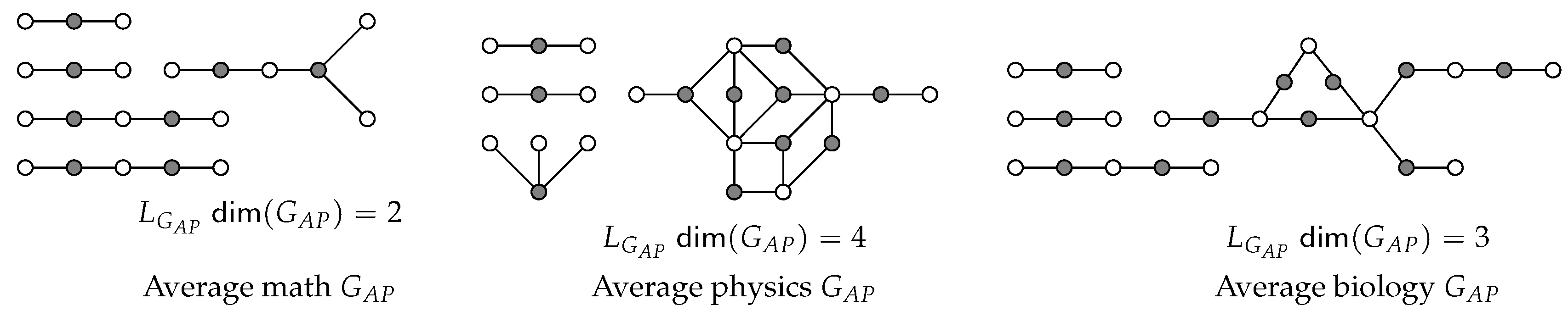
Figure 8.
The average graphs for the three disciplines.
The total number of papers produced during the study’s time frame by all considered professors was determined. On average, the physics professors produced 3.5 times as many papers as the other two research areas. In two of the physics departments, the number of representative papers outnumbered the authors by 150% due to the variety in the research group construction. Could the high level of productivity be due to the departmental collaboration style of the physics professors? Greater variety in research group construction allows for a broader range of skills and knowledge in collaborative research.
7.3. Papers Only Average Graphs and Analysis
Figure 9 clearly reflects the departmental collaboration style difference between physics and the other two research areas. Notice that the has for math, for physics and for biology.
8. The Degree Diagram and the Durfee Rank
Figure 10 displays a connected along with the degree diagrams for ’s vertex sets A and P. Although , set A has more vertices with degree 3 than P; so and . One impact of the difference in the two is that and . Can more accurately reflect the actual collaboration in a department instead of the related ? Notice that in this case.
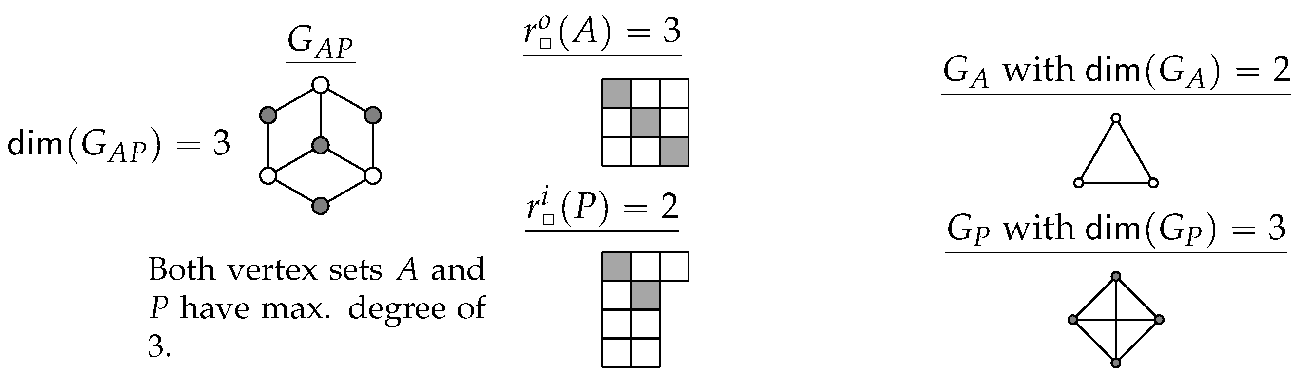
Figure 10.
with maximum degree 3 in both A and P vertex sets.
Consider the large component from a data derived depicted in Figure 11 (also displayed in Figure 6). On the top far left is the degree diagram of the degree sequence. Set has and . On the right side of are the degree diagrams for sets A and P in . Although the degree sequence for A is not graphic, each degree diagram clearly displays the degree relationships within each of the vertex sets compared to the other set. In comparing the two degree diagrams, and while and . Note that the degree diagram of is merely the union of the degree diagrams for sets A and P with and in this case.
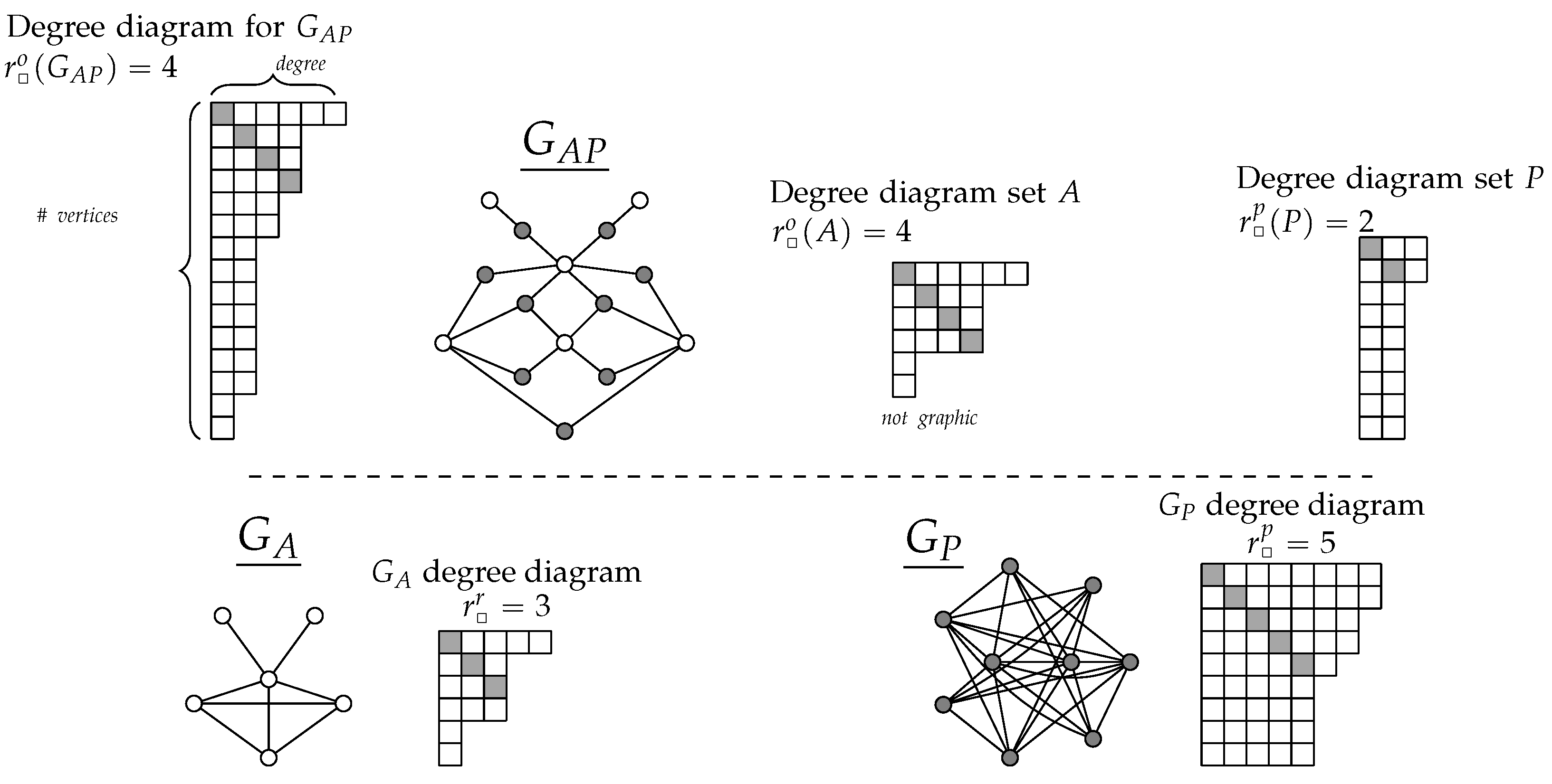
Figure 11.
Top: Data derived and the degree diagrams for , vertex set A and set P. Bottom: The related and with degree diagrams.
Figure 11.
Top: Data derived and the degree diagrams for , vertex set A and set P. Bottom: The related and with degree diagrams.
Now examine and in the lower portion of Figure 11. Here and reflecting a decrease in these figures compared to those for set A in . For , compared to and versus . This significant change is due to degree projection in where generates a subgraph in . Due to in and the Pigeonhole Principle, all of the high degree vertices are authors as shown by and . This results in all of the papers that are coauthored by the high degree authors gaining a combination of the high degrees in .
Because metric dimension is used to compare networks, and based on the change in the hubs analysis between some and their related , the next section examines the change in metric dimension given a and its related and .
9. The Metric Dimension of the Authors with Papers Graph
This section examines changes in the relative distance structure of , and , provides methods for finding . The metric dimension of G with multiple components is the sum of the metric dimension of each component in G. Although the average graphs all have multiple components, this section is focused exclusively on the changes in any single large component treated here as a connected graph. First the change between to and to for the average graphs is examined.
9.1. Changes Between the Three Data Derived Average Graphs
For each discipline, the metric dimension of that discipline’s three average graphs’ are compared. Unless otherwise stated, reference to is referring to the large component of ; and the same is true for and . The comparison begins with the mathematics discipline followed by physics and concludes with biology.
9.1.1. Metric Dimension in Average Mathematics Graphs:
With respect to the three average mathematics graphs, , and . In this case, generating a in . Thus the relative distance structures of and are similar, and the projection generating is not structure preserving with respect to the relative distance structure of even though where .
9.1.2. Metric Dimension in Average Physics Graphs:
In examining the three average physics graphs, , and with producing a subgraph in where . In this case the distance structures of and are different while the distance structures of and are similar. Here the projection generating does not preserve the relative distance structure of . This again reflects the importance of paper inclusion.
9.1.3. Metric Dimension in Average Biology Graphs:
The metric dimensions of the three average biology graphs are , and . For biology, generating a in with . Similar to physics, the relative distance structure of is that of , not .
9.2. Double Distance and Diameter
As mentioned, , is double ; and similarly for and . The double distance fact does not apply to the diameter of , and . In all cases, and due to the double distance relationship. In some cases, but not all, when the diameter in is an author to author path, then . In all cases, and since no paper can be a pendant vertex in . Recall that, by affecting the possible distance variety in a graph’s DM, diameter impacts metric dimension of a graph. When the diameter is a to a, or p to p, it is even; and when the diameter is a to p, it is odd.
9.3. Using the DM for Any Graph’S Metric Dimension
For any G with a labeling that generates distinct DM blocks, the blocks can be utilized to determine resulting in a significant increase in computational efficiency. Finding a resolving set is relatively simple. However finding a minimal resolving set is NP-hard [15] as all possibilities must be explored. Regarding a graph’s DM, all rows must be compared to all other rows in order to find a minimal number of rows that resolve G with unique column combinations. Thus, being able to find using matrix blocks gives significant computational efficiency. Theorem 9.7 states that given only three of the four DM blocks need to be resolved in order to find . Focus in this note is now on methods for finding .
9.4. DM Block Resolving
Throughout the rest of this note, it is assumed that any has a distinguishing labeling that generates blocks in its DM. As reflected in the DM blocks for any , because is bipartite, distances between elements in the same vertex set are all even, while those between the two partite sets are odd.
Definition 1.
DM block resolving is the process of using the portions of DM rows (or columns) contained in the blocks to find the minimum number of rows in each DM block that give unique column (or row) combinations.
The phrase “block resolving" is used when it is clear that the blocks are those in a DM. When using block resolving either rows, or columns, can be utilized but it is critical to use the same method for all blocks that are resolved. In this note, rows are used for block resolving and it is assumed that the reader understands that the choice of columns also exists.
All column combinations that contain a zero are unique with the zero implying that the row index vertex is in a W set for the block. The minimum number of rows that gives unique column combinations for that block is denoted by , , and .
An even block is a block that contains only even entries; so the and blocks are even. Analogously, the and blocks are odd blocks. General terms referring to the minimum number of rows that resolve a block are and . The term refers to minimally block resolving of a general block, either even or odd.
When using DM block resolving to find , the focus is on the even blocks as these blocks have row and column indices from a particular partite set, and as shown later, these block are also related to the projection graphs. The odd blocks are sometimes referred to as a block extension because literally, these blocks extend the rows of the even blocks by giving the relative distance relationships to the vertices in the other partite set.
Prior to giving four example selected for the variety of their block resolving results, the characteristics of the even and odd blocks are discussed.
9.5. DM Block Characteristics
Reference to a block row refers only to the portion of the DM row contained in the specific block being discussed.
9.5.1. Even Blocks:
Even blocks are always square and symmetric across their diagonal. The dimension of an even block is the partite set cardinality whose vertices index the block. The entries are all even with a single zero in each row, but the entries in the block compared to the block are not necessarily identical sets of even numbers.
Even blocks contain only even diameters. Because any graph has only one diameter measure, an even diameter plus the zeros, provide an even block with greater resolving efficiency by providing greater distance variety compared to its extension block. An even diameter can be in either the block only, in the block only or in both even blocks.
Recall that when row resolving, the zero indicates that that row’s index vertex is in an ordered W set, so any column combination with a zero is automatically unique. Thus the existence of the single zero automatically reduces the number of column combinations that need to be checked for uniqueness.
9.5.2. Odd Blocks
Odd blocks are only square when . The entries in the odd blocks are all odd with 1s indicating the degree of the vertex that is the row’s index. Thus, and impact the distance variety in the odd blocks while and , including their type, indicate the number of rows that might have a larger number of 1s. The odd blocks’ symmetry is to each other, across the diagonal of the DM, resulting in the two odd blocks having the same sets of odd integers. In other words, the rows of the block are the columns of the block and vice versa.
An odd diameter is in both odd blocks and increases distance variety. As extensions of the even blocks, the odd blocks can restrict the use of the related even block vertices in a minimal W set for the .
9.6. DM Block Resolving Examples
When block resolving, and always need to be determined. Based on the results of these two metric dimensions, when resolving only one more block is required. Following are four simple example with brief explanations of their block resolving.
The adjacency matrix for a , has a distinct recognizable structure of all 1s except for the all zero diagonal. The matrix resulting from is with the 1s replaced by 2s. When the structure is found as a subblock in a DM even block, it is called a double subblock. The importance of these subblocks relates back to Proposition 5.1, and the double distance relationship between and its projection graphs.
9.6.1. Example 1:
Figure 12 displays a with its DM and box that displays the metric dimension of each block.
In examining the DM in Figure 12, the entire rows for a and b have unique column combinations for all vertices in the graph as reflected by . There is a double subblock in making . The row length in is 5 but resolving two odd digits in two rows gives only unique column combinations; so the row length of 5 requires 3 rows for .
9.6.2. Example 2:
Figure 13 displays another . Both even blocks contain a double subblock and does not agree with for which the odd block is an extension.
In this case, utilizing is not possible for a minimal W in because the number of 1s in the extension block generates . Thus, a minimal W is either all three a; or three p, the choice of which depends on the rows that resolve . Note that because once these values are known, checking whether the smaller provides can be done by resolving only the extension block for the block with the smallest .
9.6.3. Example 3:
Example 3 shown in Figure 14 displays a where but is greater than .
In this case, a minimal W must be constructed with both a and p vertices; so for this example, where both DM rows contain . Utilizing three a or three p as dictated by resolves but not minimally. Thus, when all four blocks should be resolved.
9.6.4. Example 4:
As shown in Figure 15, the in Example 4 generates and .
This example provides an additional situation where and resolving the extension block for the block with the smaller provides by restricting . In other words, two a vertices do not resolve but three a give . Note that in this case and that , but . As mentioned, there is more to explore in the concept than what given in this note.
9.7. Relation of the DM Blocks to the Projection Graphs
The following proposition relates the DM blocks to the two projection graphs.
Proposition 9.1.
For the distance matrix (DM) of with authors set A and representative papers set P where has a distinguishing labeling, and .
Proof.
Because is constructed by projecting the vertices in A onto the vertices of P in the related , for each , is the number of 2s in row of the block of ’s DM. In other words, if there exists a 2 in the block at the intersection of row and column , then in because indicating that shares a neighbor p with in . Thus, if all entries in the block are multiplied by the resultant block is isomorphic to ’s DM. It follows then that a combination of rows that minimally resolve also minimally resolve . Hence, . Given , the same reasoning applies resulting in . □
Suppose that for a and its related and , and where x and y may, or may not, be equal. Due to the double distance relationship between and its projection graphs, then x number of a minimally resolve all ; but x number of a do not necessarily minimally resolve the vertices in A to those in P becuase the double distance relationship does not apply. Thus, x number of vertices do not necessarily minimally resolve . Given that , then y number of p vertices minimally resolve the vertices in P, but not necessarily minimally resolve set A nor minimally resolve .
Proposition 9.2.
Any minimal resolving set of minimally resolves the vertices but not necessarily the vertices in ; so not necessarily . Likewise any minimal resolving set of minimally resolves vertices but not necessarily the vertices in ; so not necessarily . □
9.8. Complete Graph Double Subblocks
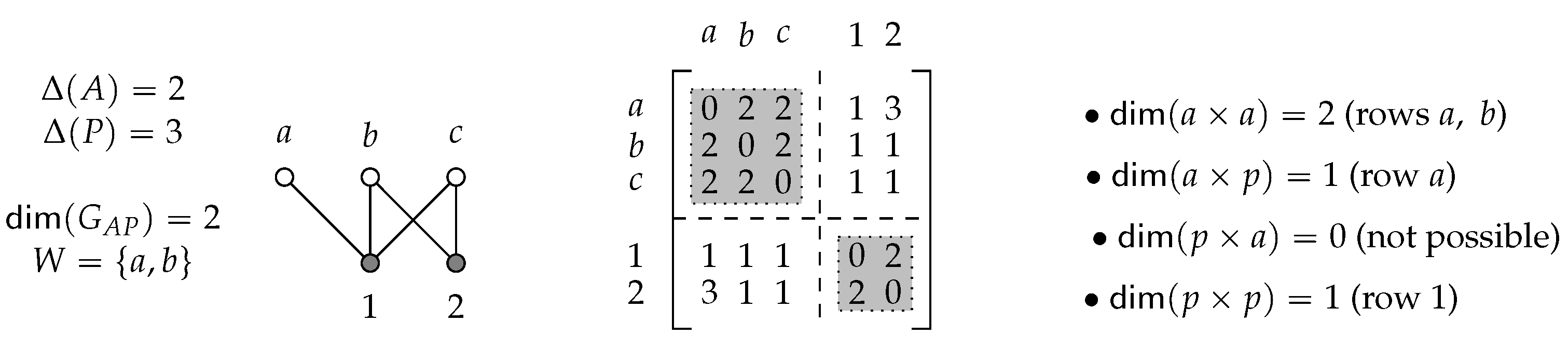
As stated previously, if a 2 is at the DM intersection of and then these vertices are adjacent in the related projection graph. If the same and are found in a double subgraph of an even DM block, then and are found in a subgraph in the related projection graph, thus impacting the metric dimension of the projection graph. Proof of the following proposition is given by the gray boxes of the DM in Figure 16.
Proposition 9.3.
Given the distance matrix (DM) for a with authors set A where and representative papers set P with , if is given a distinguishing labeling that is consecutive around its even cycle subgraphs, then a double subblock is possible in the block and a double subblock is possible in the block. □
9.9. Existence of Twin Pairs
The existence of twin pairs can affect the possible results for the DM blocks. Figure 16 shows that it is possible to have reflecting the impact of twins on block resolving.
Proposition 9.4.
Proof.
If has at least one twin a pair, by the definition of a twin pair, the rows in indexed by the twin pair have duplicate entries; and there exist duplicate columns in the block so .
When , there must exist duplicate columns in this block. Only the vertices in A can be twins; and any twin pair has identical rows in the block; so twin vertices have identical columns in the block and . If there are no twin vertices, then there are no identical columns in the block so it is resolvable and . □
Twin a vertices also generate duplicate column combinations in the block because, except for the single zero, their rows have duplicate entries and the block is symmetric along its diagonal. With their need for unique neighborhoods, no two papers can be twins. It follows then that for a , the block is always resolvable when using row block resolving. When , no W for the can contain onlyp vertices. However, p vertices can be included with a vertices in a minimal W where is determined by and
Proposition 9.5.
Suppose that a has authors set A and representative papers set P where and is not a subdivided . If then ; and if then .
Proof.
Let and . From Proposition 5.1, when , generates at least a subgraph in and generates at least a subgraph in . Corollary 5.3 states that the subgraph generated by the smaller maximum partite set degree cannot exceed the subgraph generated by the other maximum partite set degree when is not a subdivided .
When contains twins, other than the single zero in each block row, the rows of twin a vertices contain identical distances that create blocks of identical column combinations where the other a vertices have columns indexed by the twins. Thus, when , in this case can exceed the metric dimension of the double subblock and reach equality with resulting in . When , because, p vertices cannot be twins, equality does not occur. The block has at least a double subblock while the block has at least a double subblock; so . □
Because metric dimension is defined across all of G’s vertices, there exists no “efficiency" that could generate . Nor is there any inefficiency that could produce or . In other words, because is the union of A and P and both and minimally resolve the sets A and P across all of then and . This proves Lemma 9.6.
Lemma 9.6.
Suppose bipartite has authors set A and representative papers set P. Concerning the DM for , if then . □
Theorem 9.7 states that if then only three DM blocks need to be resolved.
Theorem 9.7.
For with authors set and representative paper set , with respect to block resolving ’s DM, if then resolving only three blocks determines .
Proof.
Let and where . It is a given that finding requires determining and . From Lemma 9.6. First let . As the goal is to find a minimal value for , resolving in this case gives the minimal value of a possible W for all vertices in . If then ; and if then . If contains identical rows making , and indicating the existence of twins in , then . Now let . Because is the extension of , and using the same logic as when , . In either case for x and y, only three blocks need to be resolved in order to find . □
The following proposition follows from Proposition 9.3 that shows the existence of the double subblocks.
Proposition 9.8.
Suppose has authors set A and representative papers set P. If , then .
Proof.
Suppose so . Let . If then it is a given that . If and , then because x number of a vertices minimally resolve the graph. It follows that if and then is minimally resolved by x number of p vertices so . If then a combination of a and p vertices whose numbers total x can minimally resolve giving . □
Proposition 9.9 is focused on using maximum degree and to find . Recall that indicates the degree diagram row indicated by the type and denotes the length of this row. The table in Figure 1 is referenced in the following proof of Proposition 9.9.
Proposition 9.9.
Assume that has authors set A and representative papers set P. If , and the corner type for both A and P is the same, then .
Proof.
Assume . Let where and n is odd. Because and with the same corner type, then and , , and it is a given that .
Recall that for any , . Because , the degree diagrams for both A and P have the same top row. Because and both have the same corner type, then for both diagrams, the rows above and below plus row have the same general structure as shown by the table in Figure 1. Deviation from similarity is controlled by the fact that . Thus, A and P must have very similar or identical large degree structures. From Proposition 5.1 there exists a subgraph in the projection graphs. The similarity of the large degree structures forces the degree structures of the projection graphs to deviate from the subgraph structure in similar ways. Hence, if and and the corner type for both A and P is the same, then . □
10. Possible Future Work
10.1. Social Aspects
Regarding the departments in this study, when overall papers are considered, the physics departments generate 3.5 times as many papers as either the mathematics or biology departments. Compared to the average biology and average mathematics , the average physics in Figure 8 displays large author vertex degree reflecting greater variety in the combinations of research groups based on representative papers. For two of the actual physics departments, this study revealed that the representative papers outnumbered authors by 150% indicating a greater variety in research group author inclusion. Could the physics style of departmental collaboration result in a higher paper output?
Compared to the results in [24], the percent of vertices in this note’s large components is much less. At what investigation level, does the order of the large component get close to the range 60% to 90+% inclusion found in other studies? Would exploring institutional collaboration create the large components with higher percents of inclusion?
10.2. Network Analysis Aspects
Most collaboration studies focus exclusively on the . As previously recognized in other studies, excluding papers from a collaboration network analysis results in information loss. The fact that different hubs are identified between some of this study’s compared to the related , and the fact that the interpretation of the large degree structure in is not well defined, emphasizes the need for paper inclusion since the is the actual social network. These aspects provide good foundation for Conjecture 6.1 that states determining the predicting model for collaboration network evolution, and new edge formation, requires the study of both authors and papers. Foundation for the conjecture is also found by the metric dimension analysis in this note showing that alone cannot be reliably used to predict where is the actual social network.
The challenges faced with paper inclusion in the collaboration studies based on the large databases are significant. As done in this study, utilizing representative papers reduces the number of papers; but the large number of authors on many papers poses a potential problem in defining the representative papers. Can a co-authorship “core" for papers be identified? Is there some other strategy that allows for paper inclusion without hindering collaboration network analysis due to enormous network order and size?
DM block resolving provides an accurate and more computationally efficient method for finding that clearly works for bipartite graphs. However, many networks are not bipartite. Can a method be developed, perhaps by a labeling methodology, that creates clear blocks in any graph’s DM?
References
- T.R. Anderson, R.K.S. Hankin, P.D. Killworth (2008) Beyond the Durfee square: Enhancing the h-index to score total publication output. Scientometrics 76(3). 577-588. [CrossRef]
- G.E. Andrews, K. Eriksson (2004) Integer Partitions. Cambridge Univ. press, Cambridge,UK.
- A. Anuradha, B. Amutha (2019) A study on metric dimension of some faimiles of graphs. AIP Conference Proceedings, 2019 2112 (1).
- M. Baca, E.T. Baskoro, A.N.M. Salman, S>W> Saputro, D. Suprijanto (2011) The metric dimension of regular bipartite graphs. Bull. Math. Soc. Sco. math. Roumanie Tome 54(102). No.1. 15-28.
- C.G. Blanchard, J.V. Becker, A.R. Bristow (1979) Attitudes of Southern Women: Selected Group Comparisons. Psychology of Women Quarterly 1(2). 160-171. [CrossRef]
- M.R. Carey, D.S. Johnson (1979) Computers and Intractability: A Guide to the Theory of NP-Completeness. W. H. Freeman & Co., New York, NY.
- D. Cartwright, F. Harary (1956) Structural balance: a generalization of Heider’s Theory. The Psychological Review 63(5). 277-293. [CrossRef]
- G. Chartrand, L. Ehoh, M.A. Johnson, O.R. Oellermann (2000) Resolvability in graphs and the metric dimension of a graph. Discrete Applied Mathematics 105.. 99-113. [CrossRef]
- G. Chartrand, L. Lesniak, P. Zhang (2016) Graphs & Digraphs, 6th Ed. CRC Press, Boca Raton, FL.
- C.J.Cummins, R.C. King (1987) Young diagrams, supercharacters of OSp(M/N) and modification rules. Jrnl. Phys. A: Math. Gen. 20. 3103-3120. [CrossRef]
- J. Diaz, O. Pottohen, M. Serna, E.J. van Leeuwen (2017) Complexity of metric dimension on planar graphs. Jrnl. Computer and System Sciences. 83. 132-158. [CrossRef]
- R. Diestel (2017) Graph Theory, 5th Ed. Springer: Graduate Texts in Mathematics series, Berlin, Germany.
- F. Harary, R.Z. Norman (1953) Graph theory as a mathematical model in social science. Bull. de Institut de recherches économiques et sociales (1960) 26(8).
- F. Harary, R.A. Melter (1976). On the metric dimension of a graph, Ars Combinatoria 2. 191–195.
- s. Hartung, A. Nichterlein (2013) ON the parameterized and approximation hardness of metric dimension. 2013 IEEE Conference on Computational Complexity Stanford Univ. (USA). 266–276.
- T. Heinz, P. Shapira, J.D. Rogers, J.M. Senker (2009) Organizational and institutional influences on creativity in scientific research. Research Policy 38. 610-623. [CrossRef]
- D. Janežič, A. Miličević, S. Nikolić, N. Trinajstić (2015) Graph-Theoretical Matrices in Chemistry, 2nd Ed. CRC Press, Taylor & Francis Group, Boca Raton, FL.
- S. Kyvik, I. Reyert (2017) Research collaboration in groups and networks: differences across academic fields. Scientometrics 113. 951-967. [CrossRef]
- L. Lovász (2010) Graphs and geometry. American math. Society. Volume 65.
- R. Merris (2003) Combinatorics, 2nd Ed. Wiley Interscience, John Wiley & Sons, Inc., Hoboken, NJ.
- R. Merris (2001) Graph Theory. Wiley Interscience, John Wiley & Sons, Inc.,Hoboken, NJ.
- R.K. Merton (1968) The Matthew effect in science. Science. New Series AAAS. 159(3810) 56-63.
- S. Milgram (1967) The small-world problem. psychology Today 1(1, May) 61-67.
- M. Newman (2001) The structure of scientific collaborations networks. PNAS 98(no. 2). 404-409. [CrossRef]
- M. Girvan, M.E.J. Newman (2002) Community structure in social and biological networks. PNAS-06 99(12). 7821-7826. [CrossRef]
- M. Newman (2004) Coauthorship networks and patterns of scientific collaboration. PNAS 101(1). 5200-5205. [CrossRef]
- M.E.J, Newman (2006) Power laws, Pareto distributions and Zipf’s law. arXiv:cond-mat/0412004v3 [cond-mat.stat-mech].
- M. Newman (2018) Networks, 2nd Ed. Oxford Press, Oxford, England.
- D.J. de Solla Price (1965) Networks of scientific papers: the pattern of bibliographic references indicates the nature of the scientific front. Science (American Association for the Advancement of Science) 149(3683) 510-515.
- J. Ruscio, F. Seaman, C. D’Oriano, E. Stremlo, K. Mahalchik (2012) Measuring scholarly impact using modern citation-based indices. Measurement 10. 123-146. [CrossRef]
- I. Schriba, S. Farrugia (2011) On the spectrum of threshold graphs. ISRN Discrete Math. 2011. 21 pages.
- P.J. Slater (1975). Leaves of trees (Proc. 6th Southeastern Conference on Combinatorics, Graph Theory, and Computing, Florida Atlantic Univ., Boca Raton, Fla.) Congressus Numerantium 14, Winnipeg: Utilitas Math. pp. 549–559.
- R.C. Tillquist, R.M. Frongillo, M.E. Lladser (2923) Getting the lay of the land in discrete space: a survey of metric dimension and its applications. SIAM Review 65(4). 919-962. [CrossRef]
- N. Trinajstić (1992) Chemical Graph Theory. Taylor and Francis, LLC; Boca Raton, FL.
- F.J. van Rijnsoever, L.K. hessels, R>I.J. Vandeberg (2008) A resource-based view on the interactions of university researchers. Research Policy 37.1255-1266. [CrossRef]
- C.S. Wagner, L. Leydesdorff (2005) Network structure, self-organization, and the growth of international collaboration in science. Research Policy 34. 1608-1618. [CrossRef]
- J. Wang, F. Tian,Y. Liu, J. Pang, L. Miao (2023) On graphs of order n with metric dimension n-4. Graphs and Combinatorics 39 (29) 1-18. [CrossRef]
- D.J. Watts (2003) Six degrees: the science of a connected age. W.W. Norton & Co., NYC, NY.
- D.J. Watts, S.H. Strogatz (1998) Collective dynamics of the ’small-world’ networks. nature 3393. 440-442. [CrossRef]
Figure 1.
Five types of corners and a table with respect to degree diagram row length.
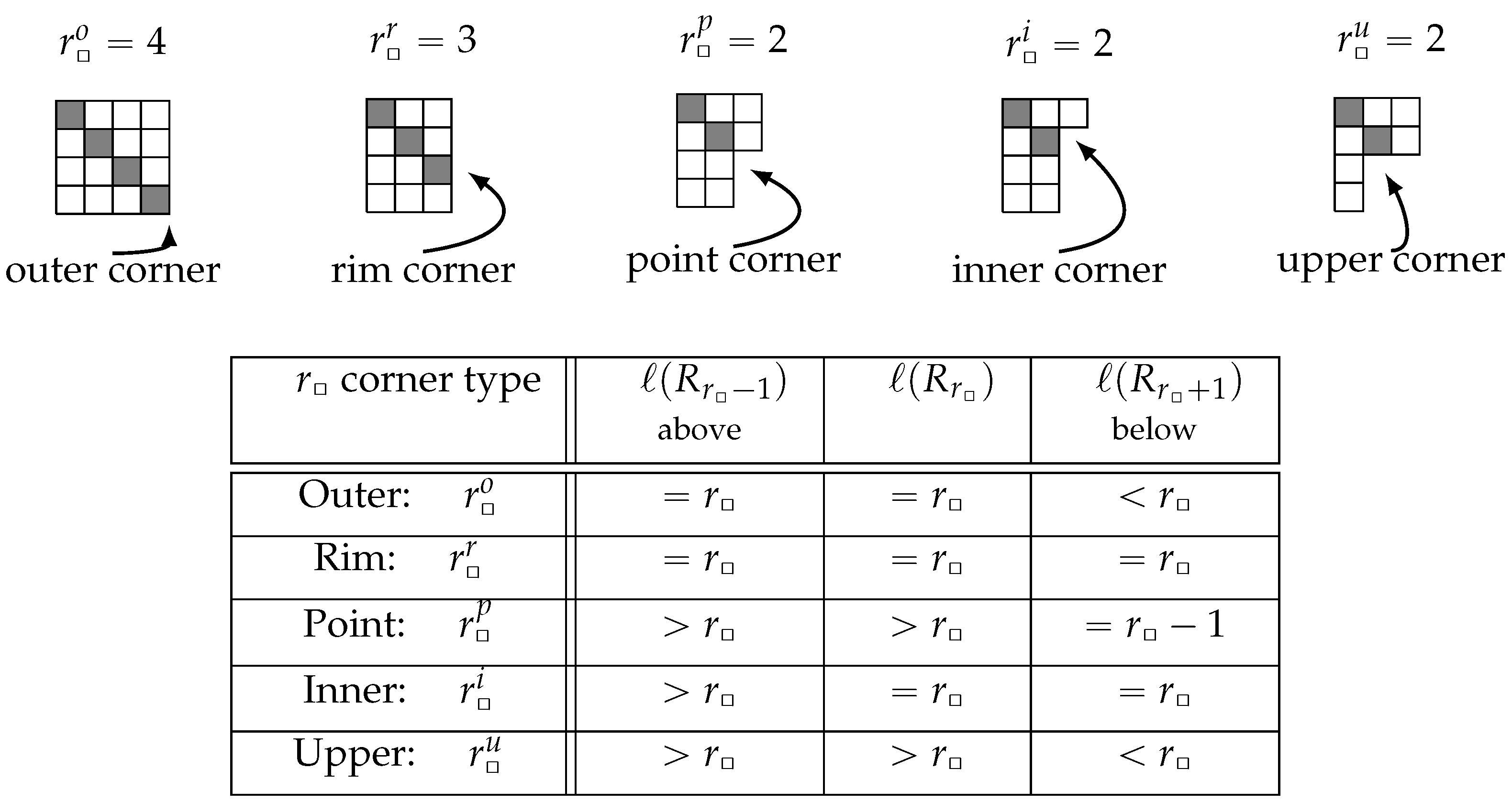
Figure 2.
Graph G and two resolving sets for G plus the distance matrix DM for G.
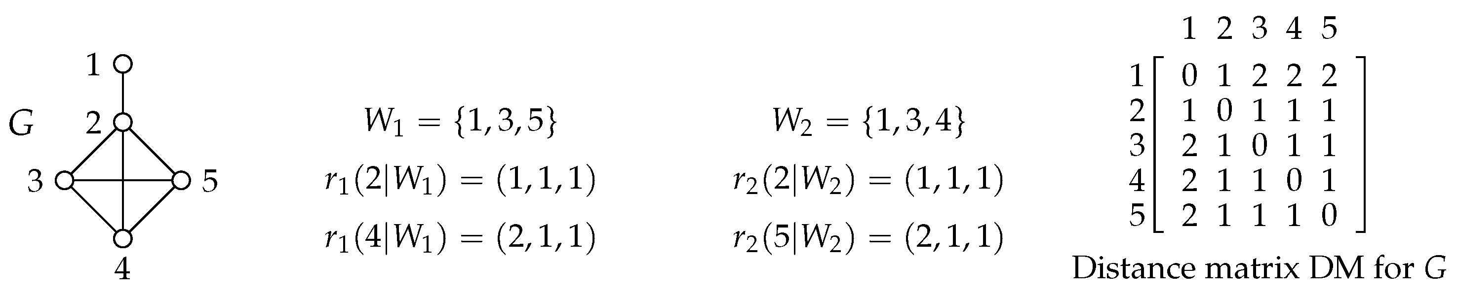
Figure 3.
Examples of largest components from data derived , and .

Figure 4.
Example with central degree 6 author and adjacent gray papers.

Figure 5.
Two with the and .
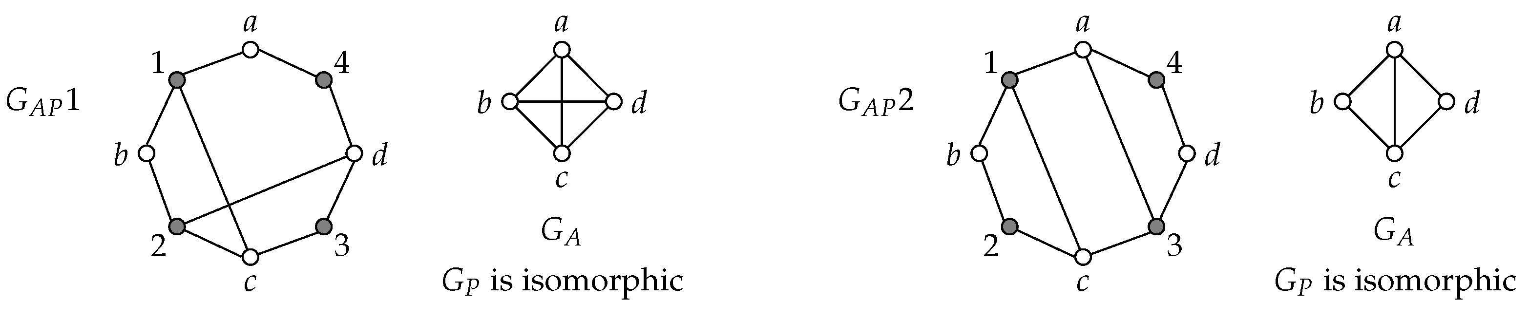
Figure 6.
A with related and .
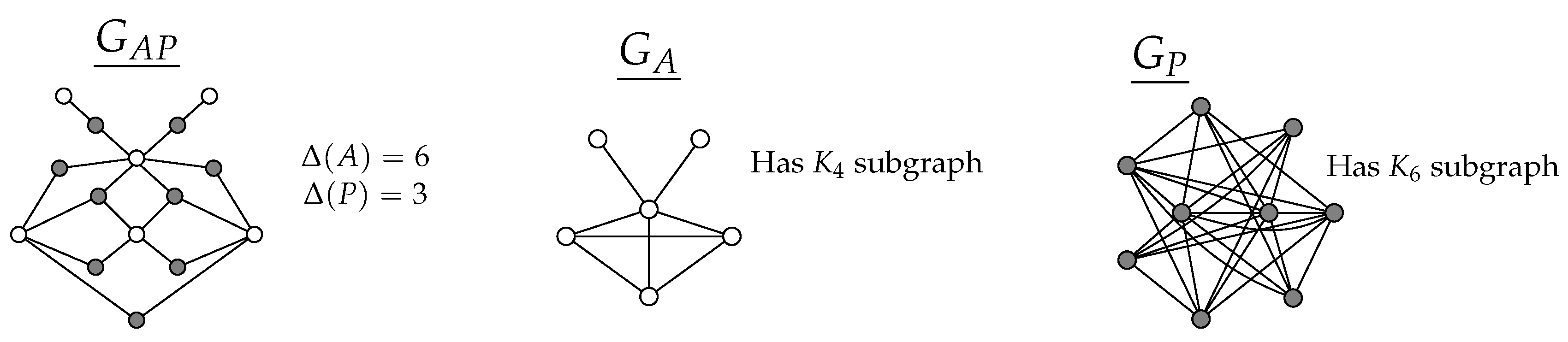
Figure 7.
The average graphs for the three disciplines.
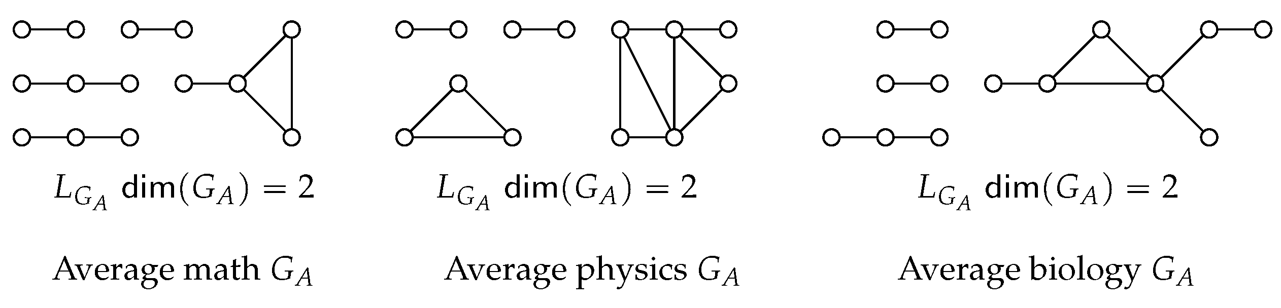
Figure 9.
The average graphs for the three disciplines.
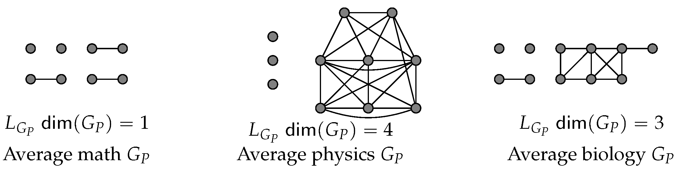
Figure 12.
Example 1 for DM block resolving.
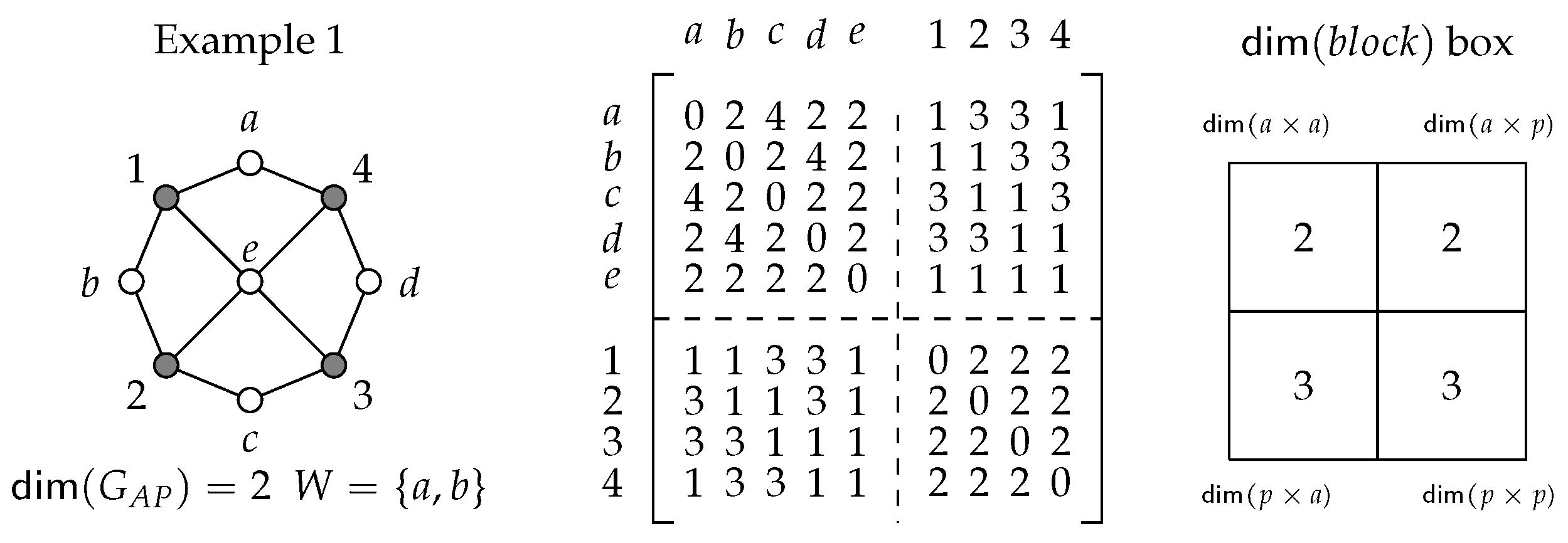
Figure 13.
Example 2 for DM block resolving.
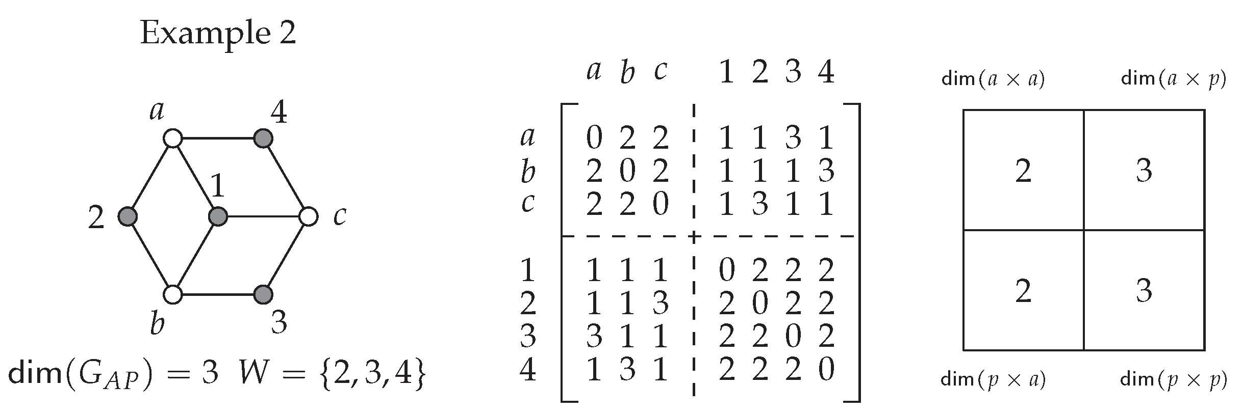
Figure 14.
Example 3 for DM block resolving.
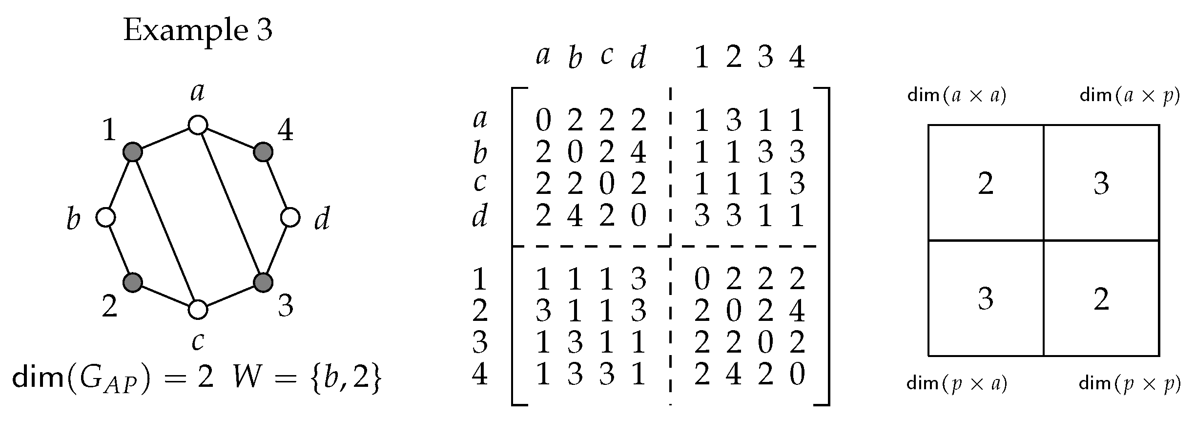
Figure 15.
Example 4 for DM block resolving.
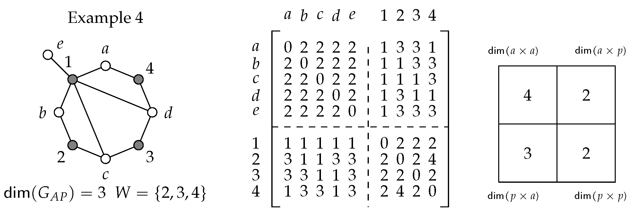

Table 1.
Faculty collaboration information for the nine departments.
| Discipline | Mean # faculty | Mean # and (%) collaborate |
|---|---|---|
| Math | 29 | 14 (48%) |
| Physics | 26 | 13 (50%) |
| Biology | 27 | 14 (52%) |
Table 2.
and hub analysis based on collected data from the nine departments.
| Discipline | Total | chair | Total | chair |
|---|---|---|---|---|
| # hubs | as hub | # hub | as hub | |
| Math | 9 | 1 | 11 | 2 |
| Physics | 5 | 1 | 9 | 0 |
| Biology | 8 | 1 | 8 | 1 |
Disclaimer/Publisher’s Note: The statements, opinions and data contained in all publications are solely those of the individual author(s) and contributor(s) and not of MDPI and/or the editor(s). MDPI and/or the editor(s) disclaim responsibility for any injury to people or property resulting from any ideas, methods, instructions or products referred to in the content. |
© 2025 by the authors. Licensee MDPI, Basel, Switzerland. This article is an open access article distributed under the terms and conditions of the Creative Commons Attribution (CC BY) license (http://creativecommons.org/licenses/by/4.0/).
Copyright: This open access article is published under a Creative Commons CC BY 4.0 license, which permit the free download, distribution, and reuse, provided that the author and preprint are cited in any reuse.