Submitted:
02 July 2025
Posted:
03 July 2025
You are already at the latest version
Abstract
Latent Heat Thermal Energy Storage (LHTES) based on phase change materials (PCM) is receiving increasing interest, since it offers high energy storage density while enabling the integration of variable renewable energies, hence boosting the transition towards a climate-neutral future. Despite the advantages that PCMs offer in providing a nearly isothermal solid–liquid phase transition, they still face some challenges that limit their deployment in real applications such as, low thermal conductivity, phase separation and supercooling, which affect charging and discharging rates. X-ray computed tomography (XCT) is a non-destructive imaging technique widely used in materials science for both qualitative and quantitative analysis of material microstructures and their evolution. Recent advances in laboratory-XCT instrumentation enabled short acquisition times on the order of tens of seconds which enable the investigation of dynamic processes in-situ by time-lapse XCT measurements. These advances open new opportunities for revealing information on the solid-liquid PCMs. Despite XCT imaging has significant potential for energy research, its application in the field of PCMs is fairly new. The present work reviews the principles of laboratory-based XCT and the recent applications of XCT technology in the characterisation of PCMs, with emphasis on the study of the solid-liquid phase transition and validation of numerical PCM models.
Keywords:
X-ray computed tomography
; solid-liquid PCM
; latent heat
; melting
; solidification
1. Introduction
Heating and cooling -mainly for industry and building - accounts for roughly half of the total energy consumed worldwide. Approximately 90% of this thermal energy comes from fossil fuel-based heating systems driving remarkable global CO2 emissions, thus demanding for effective heat decarbonization and sustainable energy technologies to achieve net-zero emission targets [1,2]. Latent heat thermal energy storage (LHTES) is a promising technology that can help significantly to reduce greenhouse gas emissions and save energy, as it enables the integration of variable renewable energy sources while balancing energy supply and demand in intermittent conditions [3,4,5]. In LHTES systems, the phase transition of a phase change material (PCM) is used for storing and releasing thermal energy (i.e., latent heat) at a nearly constant temperature (charging and discharging process) [6]. Most commonly used LHTES exploit the solid-liquid phase transition of the PCM, as it provides higher heat storage density while undergoing relatively small volumes changes between the phases [7,8,9]. Once the PCM is heated to its melting point (i.e., phase transition temperature), any further increase of thermal energy is absorbed by the material to change their internal molecular arrangement from an ordered crystalline structure (i.e.; solid phase) to a disordered randomly oriented liquid state (melting process). In reverse, when temperatures falls below the crystallisation temperature, a nucleation process starts by which molecules re-arrange into a small clusters which grow up to form a macroscopic crystalline structure, releasing the crystallisation latent heat (crystallisation process). LHTES have found applications in diverse fields at different PCMs operating temperatures, including heating and cooling of buildings [10], solar power plants [5], waste heat recovery [11] and domestic hot water systems [12]. Solid-liquid PCMs commonly used for LHTES include organic PCMs (e.g., paraffins and fatty acids) and Inorganic PCMs (e.g., salt hydrates and metal alloy), or various mixtures thereof (eutectics) [13,14,15,16].
1.1. PCM Challenges
For common latent heat applications the PCMs must behave stable during repeated solid-liquid phase transitions (i.e., thermal cycling). This repeatability requirement means that thermophysical, kinetics and chemical properties of PCMs must remain almost constant (i.e., within specific tolerance values) after repeated number of thermal cycles, to guarantee a long PCM working lifetime. However, experimental results reveal that during phase transitions (melting and solidifications) most PCMs exhibit undesired disadvantages, such as volume change (shrinkage or expansion) [9], supercooling [17], corrosion [18], leakage [19], and phases separation (i.e., incongruent melting) [20]. These effects cause significant degradation of the PCM’s thermophysical properties during thermal cycling, which limit their effective long-term performance and thus the widespread use of LHTES [21,22]. The low thermal conductivity exhibited by all traditional PCMs (e.g., about 0.2 W/m°C for paraffin), is also a major bottleneck for the PCM’s applications, since it reduces the rate of heat charging/discharging during the solid-liquid phase change [23]. To overcome theses challenges, specific solutions (e.g., thickener, nucleating agents, (micro)encapsulation, synthesis of composites, conductive additives) have been developed for specific PCMs [24,25], but they still rely on trial-and-error procedures without guaranteeing long-term cycling stability in most cases [26,27].
1.2. PCM Characterization Techniques
Accurate characterisation of the PCM’s properties is essential for the deployment of such materials into the market. Data from thermophysical properties are commonly acquired using differential scanning calorimetry (DSC), temperature history (T-History) and thermo-gravimetric analysis (TGA) techniques [28,29]. Among them, DSC has been by far the most widely used one to monitor transition temperatures and the heat of fusion of the phase transitions through the analysis of the experimental DSC curve [30,31]. However, DSC cannot to give compositional, microstructural or morphological information, which is also critical to predict the PCM performance over time. For chemical stability, Fourier-Transform Infrared (FT-IR) spectroscopy is frequently used to assess changes in the chemical structure after repeated thermal cycles [32]. X-ray powder diffraction (XRPD) and Scanning Electron Microscopy (SEM) are commonly used for assessment of crystallinity (phase identification) and morphology in hybrid PCM composites before and after cycling [33,34]. A major draw-back of these wide-spread methods, however, is that they are either destructive or measure only global bulk properties or property distributions with poor spatial resolution. In addition to that, SEM imaging, reveals morphological information on a very small region compressed a single surface and XRPD analysis is limited to crystalline materials and small sample volumes.
In recent years, X-ray computed tomography (XCT) developed into a standard technique for the volumetric, non-destructive imaging of materials [35,36]. XCT is an image technique in which X-ray projection images of a sample acquired from different directions are used to reconstruct the inner structure of the sample as a grey value distribution map of the linear X-ray attenuation coefficient. Thus, providing visualisation and volumetric imaging data of the internal 3D-structure of the sample at high spatial resolution (i.e., ∼ few microns). This is one of the main advantages of XCT compared with other destructive and 2D visualisation techniques such as SEM, optical microscopy, etc. Recent advances in XCT instrumentation [37,38] have enabled short acquisition times (∼ tens of seconds) allowing to perform in-situ XCT experiments and therefore tracking dynamic processes by time-lapse measurements. Due to this capability and the ability to precisely capture the multiscale structure of materials, XCT has found a wide range of application in materials science, leading to insights into materials properties, performance and manufacturing processes [39,40,41,42]. Despite XCT imaging has significant potential for energy research, its application in the field of PCMs is groundbreaking. The present work reviews the recent applications of laboratory-based XCT technology in characterisation of PCMs, with emphasis on the study of the solid-liquid phase transition. The objective is to highlight the potential of XCT to monitor the melting fronts, accurate quantification of solid/liquid phases, and volume changes in PCM and validation of numerical PCM models. This provides a novel rout to study non-destructively the microstructure of PCMs during the solid-liquid phase transition and thus contribute to proper designs of LHTES.
2. X-Ray Computed Tomography
2.1. XCT Workflow
To perform CT experiment, most conventional laboratory-based XCT systems employ a cone-beam acquisition geometry consisting of an X-ray source emitting a broad polychromatic X-ray beam, a rotatory stage where the sample is mounted and a detector which record the transmitted X-ray signals across the sample (cf. Figure 1). The XCT workflow is subdivided into three stages: data collection, image reconstruction, and image processing [35]. In the data collection stage, 2D X-ray radiographies are generated by impinging the beam from the X-ray source through the sample. Further, a 2D detector receives a large number of radiographic (projection) images at different angular positions during a 360° rotation of the sample. This process is usually called CT scan and could take from few minutes to hours depending on the XCT instrument, measurement parameters and the resolution required. During the reconstruction, the "projected" dataset is converted into a 3D volumetric data, using the widely-used FDK (Feldkamp, Davis, Kress) algorithm [43] or iterative reconstruction methods implemented in frameworks such as XAID from MITOS [44]. Image processing mainly involves, visualisation, filtering, segmentation, feature extraction and quantification of morphological characteristics such as phase fractions, pore networks particle size and shapes through thresholding or AI-based algorithms for subsequent quantitative analysis [46].
2.2. Attenuation Contrast Imaging
The reconstructed data provides a digital 3D grayscale representation (tomogram) of the internal structure of the sample, as a stack of cross-sectional slices which can be virtually sliced in any direction. Each reconstructed slice is a map of the linear attenuation coefficient for the corresponding section of the sample, provided that the attenuation of the X- ray beam caused by absorption is the only interaction mechanism of X-rays with matter considered. Based on this assumption, the values are retrieved using suitable algorithms from the collected projections, a line integral expressed in integral form of Beer-Lambert law as,
where is the material attenuation coefficient at position s along the path length L, and and the input and transmitted (detected) X-ray intensities, respectively [35].
The linear attenuation coefficient expresses the rate by which X-rays are attenuated as they pass through the material, thus it depends on both the material composition and the X-ray spectrum. It increases with increasing the electron density and decrease when increasing the X-ray energy. The denser the constituent material, the higher the attenuation and the brighter it will appear on the greyscale image. Therefore, material phases with sufficient density differences (e.g. solid and liquid phases of PCMs) will produce enough attenuation contrast to be distinguished from each other in the tomogram. When density differences of materials phases are too small (e.g., ), the attenuation contrast among them will be poor, therefore, other imaging modalities exploiting different interaction between X-ray and mater (e.g., phase contrast imaging) would be more suitable for the study in such a case [47].
2.3. Spatial Resolution
The spatial resolution in tomographic imaging (i.e., smallest distance at which two features can be distinguished) is mainly dependent on the achievable voxel size and the focal-spot size of the X-ray source. It measures how well small structures or the interface between of two materials phases are detected. The smaller the voxel and focal-spot size the higher the spatial resolution, thus the better representing small details in the images. To accurately characterise the image data, both voxel and focal-spot size must be significantly smaller than the smaller feature of interest in the material. The spatial resolution is typically larger than the voxel size s given by the ratio of the detector pixel size p to the geometric magnification M, i.e. . M is equal to the ratio of focus-detector distance () and focus-object distance () (cf. Figure 1). Smaller voxel sizes are achieved by increasing M (i.e., placing the sample closer to the source and farther from the detector) and/or using a detector with higher resolution. Selecting a smaller voxel size usually means accepting a smaller sample size as this generally means recording a smaller field of view (FoV) on the detector. The minimum achievable voxel size, , is determined by the ratio of the sample size (i.e., widest diameter d of the sample) to the detector size D (i.e., maximum FoV): . The focal spot, on the other hand, is an intrinsic property of the X-ray tube and its size is dependent on key parameters such as the acceleration voltage v and tube current i. In microfocus XCT systems (-CT), it lies in the micrometre range and increases with increasing the tube power, . The focal-spot size should always be smaller than the voxel size to avoid image blurring [35].
2.4. CT-Acquisition Parameters and Image Quality
Optimal choice of the CT image acquisition parameters is essential to achieve high-quality tomographic data. Parameters the user can set to optimise image quality include, the magnification, tube voltage, tube current, addition of filters, frame averaging, number of projections, exposure time and pixel binning. There is, however, no standard protocol for optimal parameter selection is established. The tube acceleration voltage should be high enough to guarantees sufficient X-ray transmission across all projections. However, a too high acceleration voltage could result (depending of the sample) in poor contrast attenuation and degraded spatial resolution, as it increases both the mean energy of the X-ray spectrum and the focal-spot size. A low acceleration voltage, on the other hand, might lead to noised images and strong beam hardening (BH) artifacts in high-density materials, which distort the reconstructed CT data and degrade measurement accuracy. BH artifacts (e.g. streaks and cupping artifacts) can be significantly reduced by using effective X-ray beam filtration strategies (i.e, combinations of materials filters of different thickness) and appropriated data reconstruction algorithms [49,50].
Increasing the tube current (without compromising the tube power), the exposure time, the number of projections and/or the frame average (i.e., number of times each projection is repeated), increase the intensity of the X-ray beam, thus improving the signal-to-noise ratio (SNR). This leads to brighter and lower levels of noise projection images at the cost of a longer acquisition time. Conversely, shorter exposure times and fewer frame averages reduce scan time but may compromise image quality. Image quality is also impacted by the detection hardware, remarkably at low-energy imaging. Currently used energy-integrating detectors produce electronic noise (dark current) during reading out causing offset of the pixel intensity. Pixel binning (i.e., combination of adjacent pixels) helps to reduce the overall noise but at the cost of reduced spatial resolution. A better solution to image quality is offered by energy-resolved photon-counting detectors, as they provide better spatial resolution, higher SNR, faster read-out speed and eliminates electronic noise [48].
2.5. Time-Lapse XCT Imaging
Time-lapse XCT imaging, also known as 4D XCT (where time is the fourth dimension), is a technique that captures a sequence of 3D XCT scans of a sample under controlled non-ambient conditions (in-situ), at discrete time steps. This protocol generates a time-series of 3D tomograms where each tomogram is representative of the sample’s microstructure at certain instant. Graphical rendering of the tomogram time-series allows for non-destructive monitoring of microstructural changes and processes in the sample over time. The time interval between consecutive XCT scans defines the temporal resolution of the XCT series, thus determining how quickly changes in the sample can be tracked. For accurate imaging, needs to be shorter than the timescale (rate) of the process to be imaged. This avoid that structural changes occur during the acquisition of the tomogram, thus preventing blurring of the critical features in the image inducing motion artifacts [54]. The shortest time interval is limited by the XCT acquisition (scan) time, which is selected as a trade-off between scan speed and image quality.
Recent developments in laboratory XCT technology have enabled short exposure times (∼ 30 ms), enabling to acquire a 3D tomogram in tens of seconds [37,51]. This time period allows to perform in-situ time-lapsed (and in-operando) XCT experiments, to track dynamic processes occurring on the seconds-to-hours timescale (e.g., melting and solidification of PCMs) [52,53]. These advances open new opportunities for revealing information on the solid-liquid phase transition occurring in PCMs, as presented in the next sections.
3. XCT Characterisation of PCM Morphology
Understanding the morphology of PCMs is crucial for optimising the performance of thermal energy storage systems in applications like, building heating and cooling systems. X-ray computed tomography is a powerful technique for characterising the morphology of PCMs. It offers significant advantages for morphology analysis, primarily due to its ability to provide non-destructive, 3D visualisation of internal structures. This analysis enables the study of morphological features such as, distribution of solid and liquid phases, pore structure, arrangement of needle-like fibres, and shape, size and spatial distribution of crystals (cf. Figure 3). Such morphological properties can significantly influence the PCM’s properties (e.g., thermal conductivity and latent heat storage capacity) thus, the overall PCM thermal performance.
Figure 2.
3D rendering of several PCMs displaying different microstructures. (Martinez-Garcia et al. [69]).
Figure 2.
3D rendering of several PCMs displaying different microstructures. (Martinez-Garcia et al. [69]).
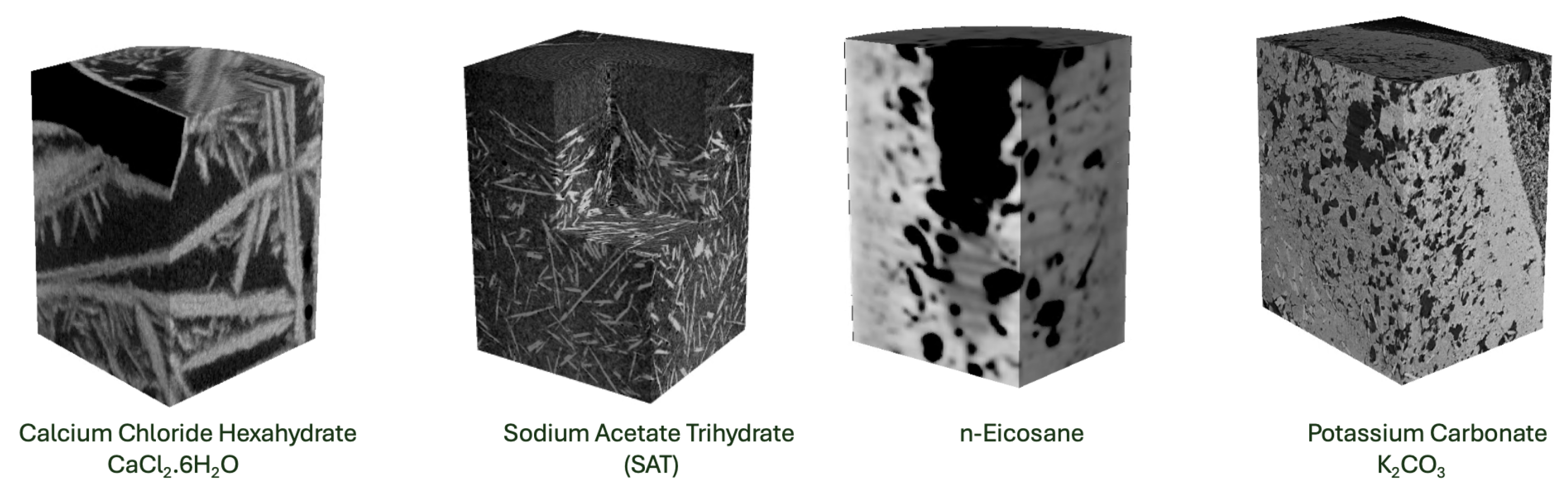
Recent applications of XCT in the field of PCMs have revealed detailed 3D information on the different kind of microstructures displayed by PCMs [69,70,71]. While commonly used salt hydrates PCMs, such as calcium chloride hexahydrate (CaCl2.6H2O) and sodium acetate trihydrate (SAT) solidify by forming different crystalline structures, organics PCM such as n-eicosane and hexadecane or even potassium carbonate (KCO3) [72] display complex pores structures of interconnected voids within a solid matrix(cf. Figs. Figure 2 and Figure 3). Further post processing of the experimental 3D image data allows for measuring and quantify the microstructure and correlate it with the PCM effective properties [68,74].
Dannemand et. al [68] used XCT to investigate the internal microstructure of two core samples SAT PCM having different degree of supercooling. One sample was seeded with SAT as it cooled down to ambient temperature to minimize supercooling, while the other was let to cool down to ambient temperature before a seed SAT crystal was added to initiate the solidification. Tomographic measurements were conducted in a commercial Zeiss Xradia 410 versa XCT system operated with acceleration voltage of 40kV. Visual inspection of the output tomographic data revealed a remarkable different microstructure between the samples (see Figure 4). Further image analysis showed that the sample, which had solidified from supercooled state contained 15% air/cavity and a sample which had solidified with minimal supercooling contained 9 % air/cavity. In both sample types the majority of the cavities were connected.
X-ray computed tomography has been also used in characterising hybrid PCM composites, aiding to find optimal container shapes (i.e, capsules, metal/carbon skeletons) to stabilise and thermally enhance the PCM [73,74,75]. Liao et. al [73] , for example, used XCT to characterise the morphology of new type of NaCl-Al2O3@SiC@l2O3 macrocapsule developed to address low thermal conductivity and easy leaks. Thermal storage macrocapsules consisted of a double-layer encapsulation of silicon carbide and alumina and a self-standing core of NaCl-Al2O. Inspection of the XCT cross-sections revealed the existence of a notable gap between the SiC coating and the Al2O ceramic shell. The SiCO displayed some degrees of cracking, potentially due to the rapid expansion of NaCl PCM during melting, forcing the SiC layer to expand. The NaCl-Al2O core maintained its spherical shape with negligible deformation when compared to its pre-heating state (cf. Figure 5).
4. XCT Analysis of Solid-Liquid Phase Changes
Time-lapse XCT enables the non-destructive monitoring of changes in the internal structure of materials and processes over time, by capturing a series of 3D images at time intervals. Advances in XCT equipment now enable short acquisition times, making it suitable for in-situ studies of dynamic processes like melting and solidification in real-time as they occur. This measurement modality is particularly useful to investigate the behavior of PCMs during repeated melting and crystallisation cycles, enabling researchers to track changes in solid/liquid fractions, volume, melting front, crystal growth, and melting and solidification rates, during the solid-liquid phase change. Therefore, to better understand phenomena like supercooling, phase segregation, and void formation, which degrade the PCM performance by reducing its heat storage capacity. Existing research on this topic in the literature is summarised below for each investigated PCM.
4.1. Magnesium Chloride Hexahydrate MgCl2.6H2O
Kohler et al.[59] used time-lapse XCT for first time to study the melting and crystallisation behaviour of PCMs, using magnesium chloride hexahydrate (MgCl2.6H2O) as case of study. The MgCl2.6H2O sample was inserted in an outer closed shell of an aluminium tube reactor designed with six thermocouples sensors positioned at different heights for temperature record. Tomographic measurements were conducted in a custom-designed CT scanner with X-ray source operated with acceleration voltage of 140 kV. A series of tomograms with voxel size of 80 x 80 x 60 m, and spatial resolution of 160 m were collected with temporal resolution of , for three melting and crystallisation cycles.
Transient temperature profiles obtained for all thermocouples revealed only negligible supercooling effects (cf. Figure 6a). Melting and crystallisation temperatures were found to be close one from each other and in good agreement with the value reported in the literature (117°C) (cf. Figure 6b). It was also concluded that not phase segregation occurred in the reactor, as only liquid PCM and solid PCM phases were observed in the XCT cross-sections image during melting and solidification (cf. Figure 6 c-d). This was also supported by the constant melting temperature measured during melting. The crystallisation process occurred non homogeneously with the formation of two crystallisation fronts moving in opposite directions (i.e., from the inside to the outside and from the outer boundary to the inside), leading to the formation of a ring channel (filled of gas) which gets narrower down the reactor until it vanishes (cf. Figure 6d). A volume change of 8% was found.
4.2. Calcium Chloride Hexahydrate CaCl2.6H2O
Martinez-Garcia et al. [61,62] studied and quantified the crystallisation dynamics of CaCl2.6H2O PCM using time-lapse XCT measurements and image processing techniques. The CaCl2.6H2O (60 g) sample was inserted into a glass vial sealed afterwards with an airtight screw on cap and fully melted using a water bath at 50°C, before placing it in the XCT device. The time-lapse XCT tomographic experiment was performed on a Diondo d2 X-ray CT system (called LuCi [45]) from Diondo, Hattingen, Germany, where the sample was placed and allowed it to solidify spontaneously, as its temperature decreased below its freezing point (29°C). A sequence of 3D tomograms with isotropic voxel size of 103 µm were collected with measurement time 7min. Measurements were conducted in high power mode using an acceleration voltage of 160 kV and a filament current of 188 µA.
The density difference between solid and liquid PCM phases was sufficient to clearly differentiate both phases in the XCT cross-section images (cf. Figure 7a). The sequence of XCT images showed that CaCl2.6H2O PCM transitioned directly from liquid to solid sate without any evidence of intermediate phase segregation. A volume reduction of 12.7 % took place through the formation of a time-growing shrinkage cavity at the top of the container. Semi-transparent 3D rendering of the segmented XCT images allowed to see internal snapshots of the crystallisation process. They showed that crystallisation of CaCl2.6H2O occurs inwards, through the junction of crystalline structures initially appearing at the side and at the bottom of the sample (cf. Figure 7b). The authors also quantified the crystallization dynamic, through measured transient liquid fraction and crystal size from the collected XCT image data. The volumetric PCM-liquid fraction curve revealed an incompleted linear solidification process with an average volumetric solidification rate of - 0.30 (%vol)/min, increased after 5.4 h to - 0.11 (% vol)/min (cf. Figure 7c). The incompleteness was evidenced by the presence of a small amount of liquid CaCl2.6H2O (2.2%), that remains until the end of the experiment. The crystal growth, on the other hand, was assessed by measuring the size of the biggest crystal over time. It was found that the growth process for this crystal occurs in three different stages. In the initial stage, a sudden occurrence of the crystal cluster take place during the first 34 min, where the biggest crystal reaches the size of roughly 2.25 cm. Afterward, the crystal growing speed decreases and the growth process runs roughly linear during the next 247 min, until it reaches a saturation stage where the crystal reaches a maximum size of 4.48 cm (cf. Figure 7d).
Guarda et al. [65] extended the study of Martinez-Garcia et al. [61,62], by providing correlated temperature data and micro-tomography XCT images for CaCl2.6H2O PCM. This extension enabled the possibility to study supercooling in CaCl2.6H2O, as done previously by Kohler et al.[59] for MgCl2.6H2O PCM. In addition, this work provided a repeatability assessment of XCT measurements. Time lapse-XCT measurements were conducted as by Martinez-Garcia et al. [61] but with optimised acquisition parameters (see Guarda et al. [65], Table 2), and time resolution of 6 min. A major difference with previous works, was the use four fibre optical temperature sensors positioned at different positions of the sample, to record PCM temperature data. The choice of fibre optical probes against thermocouples (Kohler et al.[59]), was supported by the reduction of metal artifacts in the XCT data. Sequences of XCT images displayed - in overall- similar solidification patterns for each considered case. Major differences occurred at the beginning of the crystallisation, as a consequence of the stochastic nature of crystal nucleation (cf. Figure 8a). Computed liquid fraction curves, however, matched perfectly well one with each other (cf. Figure 8b), demonstrating that XCT measurements can achieve high repeatability when using rigorous protocols and optimised settings. The temperature measurements indicated a supercooling of 2–2.5 K (cf. Figure 8c).
4.3. Ice as PCM
Martinez-Garcia et al. [60,61] and Guarda et al. [63] developed an imaged-based approach to quantify dynamic parameters during solid-liquid phase transitions in PCMs. The approach focuses on tracking the solid-liquid interface and determining key parameters like melting front speed, volumetric solid/liquid fraction and melting/solidification rate, and was first applied to the case of ice melting [63]. The sample used here was water freeze at -18 °C within a hole of diameter 20 mm and height 25mm in a holder made of extruded polystyrene foam (XPS from Swisspor, Boswil, Switzerland). Time-lapse XCT measurements were conducted on a Diondo d2 X-ray CT system (LuCi [45]) where the sample was placed at allowed to melt at ambient temperature (20 °C). A sequence of 3D tomograms with isotropic voxel size of 84µm were collected with measurement time 6min. The measurements were conducted in high power mode with an operation voltage of 160 kV and a filament current of 188 µA in a helical scan. The full list of used acquisition parameters can be found in Martinez-Garcia et al. [60,61].
The density difference between solid and liquid phases at 0°C is about 6%, which resulted in a contrast suitable to clearly discern both phases in the XCT images (cf. Figure 9a). The computed time-dependent volumetric liquid fraction curve reveals a linear melting process occurring at a constant volumetric melting-rate of 0.58 (% vol)/min (cf. Figure 9b). From the plot it was deduced that the melting process starts at min and ends at min, thus taking around 165 min. The author also were capable to extract the melting front surface at each time step from the segmented image and calculated the average pair-wise distance between them. This was used to estimate the meting front velocity yielding a value of 2.6 m/min.
4.4. n-Eicosane C20H42
Guarda et al. [64] used time-lapse XCT imaging measurements to track the solidification behaviour of n-eicosane (organic) PCM. Different to previous works, it was necessary to perform first a sensitive analysis to optimise the XCT acquisition parameters to ensure maximum contrast between the solid and liquid eicosane phases. The sensitive analysis was then carried out by performing multiple (static) XCT scans with different combination of acceleration voltages and filters, from which the 120 kV acceleration voltage and 1.0 mm Al filter combination was chosen as optimal. Detailed information about this analysis can be found in Guarda et al. [64] (see Table 1 and Figure5 therein). Time-lapse XCT measurements were then conducted on a Diondo d2 X-ray CT system (called LuCi) [45]. A liquid eicosane sample at initial temperature 50°C was placed in rotatory stage of XCT systems and allowed to solidify while keeping the room temperature at 20 °C. A sequence of 3D tomograms with isotropic voxel size of 103 µm were collected with measurement time 5min. The full list of used acquisition and reconstruction parameters can be found in Guarda et al. [64].
The optimisation of the CT acquisition parameters led to a suitable contrast to clearly discern both solid and liquid phases and thus to track the eicosane solidifcation, as shown in Figure 10a. A distinctive feature of this study was the complex pore network structure developed by the PCM during the phase transition, which led to an overall volumetric shrinkage of ∼14.5 %. The specific pore characteristics (size, shape and distribution), which can be visualized in Figure 10c, significantly impacted the PCM’s thermal performance and required to enhancing the segmentation algorithm used to compute the volumetric liquid fraction shown in Figure 10b.
5. XCT as a Tool to Validate PCM Numerical Models
The availability of time-resolved XCT imaging data, represents a valuable tool for calibrating and validating numerical models used to design proper LHTES. Different computational models have been deployed to predict the PCM behaviour during melting and solidification [55,56]. Among them, the enthalpy-porosity method developed by Voller et al. [57,58] has been the most commonly used one, as it is computational efficient and provides accurate results for both sharp and gradual solid-liquid phase changes. Different to other numerical methods, it simplifies the simulation by treating the mushy zone (region where both solid and liquid phase coexist) as a porous medium with a porosity that varies based on the liquid fraction, which is modelled as a smooth function of the PCM temperature. The XCT-based strategy to validate numerical PCM models consist in comparing the model’s predicted liquid fraction curve with the experimental one obtained from XCT imaging data. Models parameters (e.g., time-step, mesh sensitivity, inlet temperature, heating/cooling rate, etc) should be tuned until reaching the best possible match between simulated and experimental liquid fraction curves. This is a fairly new approach that has been applied recently to the PCMs exemplified below.
5.0.1. Melting of Ice
Guarda et al. [63] made the first attempt to validate PCM numerical models against transient liquid fraction data extracted from time-lapse XCT experiments. To do that, an ice cylinder frozen at -18° was allowed to melt inside a XCT system (called LuCi) [45] and in-situ time-lapse XCT measurements during the process melting were recorded, as described in SubSection 4.3. From the time-series of tomograms, the transient volume fraction curve of water was computed by using in-house developed algorithm. This data was used to validate numerical results obtained from an enthalpy-porosity model developed for the same system and executed in Ansys Fluent 18.2 [63].
An excellent agreement between experimental and numerical liquid fractions was found, as shown in Figure 11b. The algorithm applied to calculate liquid fraction from XCT data works better in cases when liquid and solid phase are not disproportional in size. This corresponds to the time range where both model and experiments match pretty well. Comparison of liquid fraction contours between model and experiment also revealed the same trend over time (cf. Figure 11a).
5.1. Solidification of n-Eicosane
An enthalpy-porosity model developed to study n-eicosane PCM during solidification, was also validated against a transient volumetric liquid fraction curved obtained from XCT experiments [64]. The numerical model was implemented Ansys Fluent 18.2 considering an asymmetric geometry consisting of a cylindrical shaped PCM and also solid zones of its container made of extruded polystyrene (XPS). Time step and mesh sensitivity analysis were conducted to optimise the numerical model. An step size of 0.1s and a mesh of 10k (9878 mesh elements) resulted as optimal values. More details of the model and PCM properties used in the simulation can be found Guarda et al. [64]. Time-lapse XCT imaging data for the PCM were collected at time intervals of min while solidified keeping the room temperature at 20 °C, as described in Subsection 4.4 (cf. Figure 10a).
The liquid fraction evolution estimated from the simulation agrees fairly well with the liquid fraction from the dynamic XCT, particularly in the central zone, where both the solid and the liquid phases are roughly equally present (cf. Figure 10b). The mean absolute error between the experimental and numerical liquid fraction is around 5.1%.
5.2. Solidification of CaCl2.6H2O
Different from previous works, Guarda et al. [65] performed time-lapse XCT imaging of CaCl2.6H2O during solidification, capturing simultaneously temperature data through the use of four temperature sensors positioned at different height within the sample. This allowed for first time correlate the internal PCM’s microstructure with the temperature. Transient volumetric liquid fractions derived from experimental XCT and PCM’s temperature data, were successfully used to validate an enthalpy-porosity model for solid–liquid phase change largely used in multiple works [66,67].
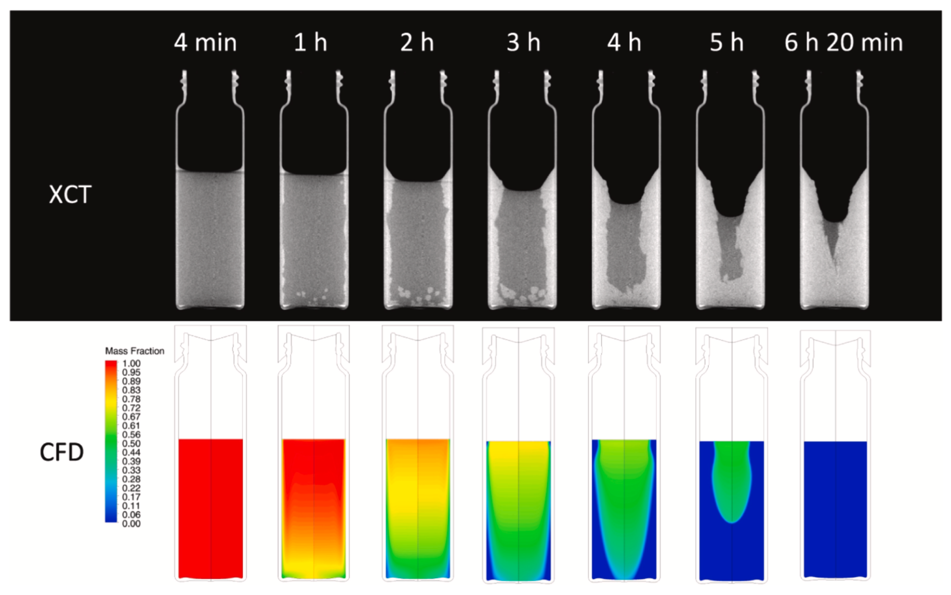
Results of the validation are shown in Figure 12(b-d). As it can be seen from the Figure, the numerical and experimental liquid fraction curves show good agreement, remarkably, in the central part of the process which occurs rather linearly. The experimental curve does not reach 0 since there is a certain amount of liquid phase left. The numerical curve, on the other hand, does not account for the liquid phase left, resulting in a complete solidification Comparison of experimental and computed temperatures (cf. Figure 12c) reveals that the simplified enthalpy-porosity model does not account neither for supercooling nor phase separation phenomena. Comparison of liquid fraction contours between model (CFD) and experiment (XCT cross-sections) also revealed the same trend over time (cf. Figure 13).
The combination of these two measurement techniques, for temperature and volumetric liquid fraction, enabled a deeper understanding and interpretation of the phase-change mechanisms. In particular, the direct coupling of the local temperature measurement with the 3D image reconstruction allows for the unprecedented analysis of the supercooling phenomenon of calcium chloride hexahydrate. This phenomenon was tracked through XCT cross-sections of sample taken close to the bottom, collected at different time points as described in Subsection 4.2 (cf. Figure 12a).
6. Challenges and Concluding Remarks
This article reviews the basic principles of X-ray computed tomography (XCT) and showcases the capabilities of lab-based XCT equipment in analysing the morphology, solid-liquid phase transition and numerical model validation of PCMs. The review demonstrates that optimised XCT acquisition combined with image processing techniques can provide accurate and relevant information about the occurrence and distribution of PCM phases during melting and solidification. Thus, enabling a direct assessment of phase segregation and volumetric changes in PCMs. In particular, it was shown how time-resolved XCT image data can be used to assess the solid-liquid phase dynamic by quantifying melting front, crystals size and transient volumetric liquid fractions. It was also shown that when correlated with experimental temperature data, XCT images can also visually represent the supercooling phenomenon, thus providing a deeper insight in its interpretation.
While laboratory-XCT has demonstrated significant capabilities in the analysis of PCMs, there are however, specific challenges that needs to be addressed during XCT of PCMs which are discussed below.
- Spatial resolution: PCM can exhibit complex microstructures during solid-liquid phase transitions, with features like micro-crystal, or micropores in the micrometer range (few micrometres in size) requiring nano-scale spatial resolution.
- Attenuation contrast: Density differences or X-ray attenuation between PCM phases (solid-liquid or solid-solid) may be subtle, making it difficult to distinguish them. In such a case other XCT imaging modalities, like phase contrast imaging, are recommended instead of conventional absorption-based XCT.
- High throughput: CT scan can still take several minutes or even up to an hour, depending on the XCT device and the detailed imaging. This could be inappropriate to image fast processes occurring on seconds-to-minutes time scale. It is here recommended to use the state of the art of XCT instrumentation combined with optimised image acquisition protocols.
- Non ambient attachment. Temperature control with temperature sensors is cumbersome and leads to potential metal artefacts which should me mitigated during the reconstruction. When possible, it is recommendable to use appropriated thermal chamber attachment enabling both temperature and heating/cooling rate control.
- Segmentation algorithms: Specialised (AI-based) segmentation algorithms may be needed in case of complex PCM microstructures (e.g., pore networks in organic PCM) to reliably differentiate between solid and liquid phases.
Sometimes lab-based XCT is enough and researchers don’t need to wait for synchrotron radiation time.
Acknowledgments
The authors would like to thank to the Swiss National Science Foundation, Switzerland for the support of the acquisition of the LuCi instrument (Grant 206021-189608) and the support of the research projects, Investigation of Salt Hydrates Segregation with XCT, Switzerland (Grant 200021–201088) and ROCS: Root Causes for Stochastic behaviour of salt hydrates (Grant 200021-232283).
Conflicts of Interest
The authors declare no conflicts of interest.
Abbreviations
| LUASA | Lucerne University of Applied Science and Arts |
| LuCi | Lucerne CT Imaging |
References
- Gilbert, T.; Menon, A. K.; Dames, C.; Prasher, R. Heat source and application-dependent levelized cost of decarbonized heat. Joule 2023, 7, 128–149. [Google Scholar] [CrossRef]
- Ang, T.-Z. et al. A comprehensive study of renewable energy sources: Classifications, challenges and suggestions. Energy Strateg Rev. 2022, 143, 100939.
- Hamzat, Abdulhammed K. et al. Phase change materials in solar energy storage: Recent progress, environmental impact, challenges, and perspectives. J. Energy Storage 2025, 114, 115762. [CrossRef]
- Mehta, P. et al. Performance assessment of thermal energy storage system for solar thermal applications. Sci. Rep. 2025, 14, 13876.
- Jayathunga, D. S.; Karunathilake, H.P.; Narayana, M. Witharana, S. Phase change material (PCM) candidates for latent heat thermal energy storage (LHTES) in concentrated solar power (CSP) based thermal applications - A review. Renew. Sustain. Energy Rev. 2024, 189, 113904. [Google Scholar] [CrossRef]
- Stamatiou, A.; Maranda, S.; Fischer, L.J.; Worlitschek, J. Solid–Liquid Phase Change Materials for Energy Storage - Opportunities and Challenges. In Solid-Liquid Thermal Energy Storage: Modeling and Applications; Mobedi, M., Hooman, K., Tao, W.-Q., Eds.; CRC Press, Taylor & Francis Group: Boca Raton, 2022; pp. 1–22. [Google Scholar]
- Zalba, B.; Marin, J.M.; Cabeza, L.F.; Mehling, H. Review on thermal energy storage with phase change: materials, heat transfer analysis and applications. Appl Therm. Eng. 2003, 23, 251–283. [Google Scholar] [CrossRef]
- Togun, H.. et al. A critical review on phase change materials (PCM) based heat exchanger: Different hybrid techniques for the enhancement. J. Energy Storage 2024, 79, 109840. [CrossRef]
- Cabeza, L.F.; Zsembinszki, G.; Martin, M. Evaluation of volume change in phase change materials during their phase transition. J. Energy Storage 2020, 28, 101206. [Google Scholar] [CrossRef]
- Sharshir, S.W. et al. Thermal energy storage using phase change materials in building applications: A review of the recent development. Energy Build. 2023, 7285, 112908.
- Lalau, Y.; Rigal, S.; Bedecarrats, J.P.; Haillot, D. Latent Thermal Energy Storage System for Heat Recovery between 120 and 150 °C: Material Stability and Corrosion. Energies 2024, 14, 787. [Google Scholar] [CrossRef]
- Yang, M.; Moghimi, M.A.; Loillier, R.; Markides, C.N.; Kadivar, M. Design of a latent heat thermal energy storage system under simultaneous charging and discharging for solar domestic hot water applications. Appl. Energy 2023, 336, 120848. [Google Scholar] [CrossRef]
- Farid, M.M; Khudhair, A.M.; Razack, S.A.K.; Al-Hallaj, S. A review on phase change energy storage: materials and applications. Energy Convers. Manag. 2004, 45, 1597–1615. [CrossRef]
- Sharma, A.; Tyagi, V.V.; Chen, C.R.; Buddhi, D. Review on thermal energy storage with phase change materials and applications. Renew. Sust. Energ. Rev. 2009, 13, 318–345. [Google Scholar] [CrossRef]
- Cabeza, L.F.; Castell, A.; Barreneche, C.; de Gracia, A.; Fernandez, A.I. Materials used as PCM in thermal energy storage in buildings: A review. Renew. Sust. Energ. Rev. 2011, 15, 1675–1695. [Google Scholar] [CrossRef]
- Reddy, K.S.; Mudgal, V.; Mallick, V.M. Review of latent heat thermal energy storage for improved material stability and effective load management. J. Energy Storage 2018, 15, 205–227. [Google Scholar] [CrossRef]
- Shamseddine, I.; Pennec, F.; Biwole, P; Fardoun, F. Supercooling of phase change materials: A review. Renew. Sust. Energ. Rev. 2022, 158, 112172. [Google Scholar] [CrossRef]
- Hua, W.; Xu, X.; Zhang, X; Yan, H.; Zhang, J. Progress in corrosion and anti-corrosion measures of phase change materials in thermal storage and management systems. J. Energy Storage. 2022, 56, 105883. [Google Scholar] [CrossRef]
- Aulakh, J.S.; Joshi, D.P. Thermal and Anti-Leakage Performance of PCM for Thermal Energy Storage Applications. In Recent Advances in Nanotechnology.; Khan, Z.H., Jackson, M., Salah, N.A., Eds.; ICNOC 2022; Springer Proceedings in Materials vol 28: Singapore, 2023; pp. 235–241. [Google Scholar]
- Tan, P.; Lindberg, P.; Eichler, K; Löveryd, P.; Johansson, P.; Kalagasidis, A.S. Effect of phase separation and supercooling on the storage capacity in a commercial latent heat thermal energy storage: Experimental cycling of a salt hydrate PCM. J. Energy Storage 2020, 29, 101266. [Google Scholar] [CrossRef]
- Anand, A.; Shukla, A.; Kumar, A.; Buddhi, D.; Sharma, A. Cycle test stability and corrosion evaluation of phase change materials used in thermal energy storage systems. J. Energy Storage 2021, 39, 102664. [Google Scholar] [CrossRef]
- Ferrer, F.; Solè, A.; Barreneche, C.; Martorell, I.; Cabeza, L.F. Review on the methodology used in thermal stability characterization of phase change materials. Renew. Sust. Energ. Rev. 2015, 50, 665–685. [Google Scholar] [CrossRef]
- Xu, C.; Zhang, A.; Fang, G. Review on thermal conductivity improvement of phase change materials with enhanced additives for thermal energy storage. J. Energy Storage 2022, 51, 104568. [Google Scholar] [CrossRef]
- Li, Y. et al. Stable salt hydrate-based thermal energy storage materials. Compos B Eng. 2022, 233, 109621. [Google Scholar] [CrossRef]
- Chakraborty, A. et al. Stable salt hydrate-based thermal energy storage materials. J. Energy Storage 2022, 52, 104856. [Google Scholar] [CrossRef]
- Akamo, D.O.; Noh, J.; March, R.; Shamberger, P.; Yu, C. Thermal energy storage composites with preformed expanded graphite matrix and paraffin wax for long-term cycling stability and tailored thermal properties. iScience 2023, 26, 107175. [Google Scholar] [CrossRef] [PubMed]
- Kant, K.; Bowole, P.H.; Shamseddine, I; Tlaiji, G.; Pennec, F.; Fardoun, F. Recent advances in thermophysical properties enhancement of phase change materials for thermal energy storage. Energy Mater. Sol. Cells 2021, 231, 111309. [Google Scholar] [CrossRef]
- Cabeza, L.F. et al. Unconventional experimental technologies available for phase change materials (PCM) characterization. Part 1. Thermophysical properties. Renew. Sust. Energ. Rev 2015, 43, 1399–1414. [Google Scholar] [CrossRef]
- Müller, L. et al. Consistent DSC and TGA Methodology as Basis for the Measurement and Comparison of Thermo-Physical Properties of Phase Change Materials. Materials 2020, 13, 4486. [Google Scholar] [CrossRef]
- Fatahi, H.; Claverie, J.; Poncet, S. Thermal Characterization of Phase Change Materials by Differential Scanning Calorimetry: A Review. Appl. Sci. 2022, 12, 12019. [Google Scholar] [CrossRef]
- Martínez, A.; Carmona, M.; Cortés, C.; Arauzo, I. Characterization of Thermophysical Properties of Phase Change Materials Using Unconventional Experimental Technologies. Energies. 2020, 18, 4687. [Google Scholar] [CrossRef]
- Solé, A. et al. Stability of sugar alcohols as PCM for thermal energy storage. Sol. Energy Mater. Sol. Cells 2014, 126, 125–134. [Google Scholar] [CrossRef]
- Fernandéz, A. I. et al. Unconventional experimental technologies used for phase change materials (PCM) characterization: part 2– morphological and structural characterization, physico-chemical stability and mechanical properties. Renew. Sust. Energ. Rev 2015, 43, 1415–1426. [Google Scholar] [CrossRef]
- Huang, X.; Alva, G.; Jia, Y.; Fang, G. Morphological characterization and applications of phase change materials in thermal energy storage: A review. Renew. Sust. Energ. Rev 2017, 72, 1128–145. [Google Scholar] [CrossRef]
- Carmignato, S.; Dewulf, W.; Leach, R. Industrial X-ray computed tomography; Springer: Cham, Switzerland, 2018. [Google Scholar]
- Withers, P. J.; Bouman, C.; Carmignato, S. et al. X-ray computed tomography. Nat Rev Methods Primers 2021, 1, 18. [Google Scholar] [CrossRef]
- Vǎvrík, D.; Jakøubek, J.; Kumpova, I.; Pichotka, M . Laboratory based study of dynamical processes by 4D x-ray CT with sub-second temporal resolution. J. Instrum. 2017, 12, C02010. [Google Scholar] [CrossRef]
- Yuki, R.; Ohtake, Y.; Suzuki, H. Acceleration of X-ray computed tomography scanning with high-quality reconstructed volume by deblurring transmission images using convolutional neural networks. Precis. Eng. 2022, 73, 153–165. [Google Scholar] [CrossRef]
- du Pleiss, A.; Yadroitsev, I.; Yadroitsava, I.; Le Roux, S. G. X-Ray Microcomputed Tomography in Additive Manufacturing: A Review of the Current Technology and Applications. 3D Print. Addit. Manuf. 2018, 5, 227–247. [Google Scholar] [CrossRef]
- Sun, X. , et al. X-ray computed tomography in metal additive manufacturing: A review on prevention, diagnostic, and prediction of failure. Thin Walled Struct. 2025, 207, 112736. [Google Scholar] [CrossRef]
- Martinez-Garcia, J.; Braginsky, L.; Shklover, V.; Lawson, J. W. Correlation function analysis of fiber networks: Implications for thermal conductivity. Phys. Rev. B 2011, 84, 054208. [Google Scholar] [CrossRef]
- Gebhard, M. et al. X-Ray-Computed Radiography and Tomography Study of Electrolyte Invasion and Distribution inside Pristine and Heat-Treated Carbon Felts for Redox Flow Batteries. Energy Technol. 2020, 8, 1901214. [Google Scholar] [CrossRef]
- Feldkamp, L.; Davis, L. C.; Kress, J. Practical cone-beam algorithm. J. Opt. Soc. Am 1984, 1, 612–9. [Google Scholar] [CrossRef]
- https://x-aid.de.
- https://www.hslu.ch/luci.
- Maire, E.; Withers, P. J. Quantitative X- ray tomography. Int. Mater. Rev. 2014, 59, 1–43. [Google Scholar] [CrossRef]
- Endrizzi, M. Practical cone-beam algorithm. Nucl. Instrum. Methods Phys. Res. Sect. A 2018, 878, 88–98. [Google Scholar] [CrossRef]
- Martinez-Garcia, J. et al. Energy-selective X-ray CT imaging with an EIGER2 hybrid photon counting detector in a Diondo d2 XCT system. e-Journal of Nondestructive Testing. 2024, 29, 1–6. [Google Scholar] [CrossRef] [PubMed]
- Yang, F.; Zhang, H.; Huang, K. Cupping artifacts correction for polychromatic X-ray cone-beam computed tomography based on projection compensation and hardening behavior. Biomed. Signal Process. Control 2020, 57, 101823. [Google Scholar] [CrossRef]
- Trotta, L. et al. Beam-hardening corrections through a polychromatic projection model integrated to an iterative reconstruction algorithm. NDT&E INT. 2022, 126, 102594. [Google Scholar]
- Eggert, A. et al. High-speed in-situ tomography of liquid protein foams. Int. J. Matter. Res. 2014, 105, 632–9. [Google Scholar] [CrossRef]
- Dziȩciołl, K., L. et al. Laboratory X-ray computed tomography imaging protocol allowing the operando investigation of electrode material evolution in various environments. iScience. 2023, 26, 107097. [Google Scholar] [CrossRef]
- Zwanenburg, E., A.; Williams, M. A.; Warnett, J. M. Review of high-speed imaging with lab-based x-ray computed tomography. Meas. Sci. Technol. 2021, 33, 012003. [Google Scholar] [CrossRef]
- Davis, R. G.; Elliot, J. C. Artefacts in X-ray microtomography of materials. Mater. Sci. Technol. 2006, 22, 1011–1016. [Google Scholar] [CrossRef]
- Uzan, A. Y.; Kozak, Y.; Korin, Y.; Haray, I.; Mehling, G.; Ziskind, G. A novel multi-dimensional model for solidification process with supercooling. Int. J. Heat Mass Transf. 2017, 106, 91–102. [Google Scholar] [CrossRef]
- Khattari, Y.; El Rhafiki, T.; Choab, N.; et al. Apparent heat capacity method to investigate heat transfer in a composite phase change material. J. Energy Storage 2020, 28, 101239. [Google Scholar] [CrossRef]
- Voller, V. R. An enthalpy method for convection/diffusion phase change. Int. J. Numer. Methods Eng. 1987, 24, 271–284. [Google Scholar] [CrossRef]
- Voller, V. R.; Swaminathan, C. R.; Thomas, B. G. General source-based method for solidification phase change. Numer. Heat Transf. Part Fundam. 1991, 19, 175–189. [Google Scholar] [CrossRef]
- Kohler, T.; Kögl, T. Study of the Crystallization and Melting Behavior of a Latent Heat Storage by Computed Tomography Chem. Ing. Tech. 2018, 90, 366–371. [Google Scholar] [CrossRef]
- Martinez-Garcia, et al. Fully volumetric tracking of melting processes in phase change materials with computed tomography. In: Proceedings of the 11th Conference on Industrial Computed Tomography (ICT), Wels, Austria, 8-11 Feb. 2022.
- Martinez-Garcia, et al. Volumetric quantification of melting and solidification of phase change materials by in-situ X-ray computed tomography. J. Energy Storage. 2023, 61, 106726. [CrossRef]
- Martinez-Garcia, et al. Study of the solidification behaviour of calcium chloride hexahydrate by in-situ X-ray computed tomography. Res. Review J. Nondestructive Testing (ReJNDDT) 2023, 1, 1.
- Guarda, D. et al. Phase Change Material numerical simulation: enthalpy-porosity model validation against liquid fraction data from an X-ray computed tomography measurement/system. Nondestruct. Test. Eval. 2022, 37, 508–518. [Google Scholar] [CrossRef]
- Guarda, D. et al. New liquid fraction measurement methodology for phase change material analysis based on X-ray computed tomography. Int. J. Therm. Sci. 2023, 194, 108585. [Google Scholar] [CrossRef]
- Guarda, D. et al. X-ray computed tomography analysis of calcium chloride hexahydrate solidification. Appl. Therm. Eng. 2024, 252, 123618. [Google Scholar] [CrossRef]
- Shmueli, H.; Ziskind, G.; Letan, R. Melting in a vertical cylindrical tube: numerical investigation and comparison with experiments. Int. J. Heat Mass Transf. 2010, 53, 4082–14091. [Google Scholar] [CrossRef]
- Fornarelli, F. et al. CFD analysis of melting process in a shell- and-tube latent heat storage for concentrated solar power plants. Appl. Energy 2016, 164, 712–722. [Google Scholar] [CrossRef]
- Dannemand, M. et al. Porosity and density measurements of sodium acetate trihydrate for thermal energy storage. Appl. Therm. Eng. 2018, 131, 707–714. [Google Scholar] [CrossRef]
- Martinez-Garcia, J. et al. X-ray computed tomography image processing of solid-liquid PCMs with Geodict. In: Proceedings of GeoDict Innovation Conference 2024, Ramstein, Germany, 6-7 Feb 2024.
- Stamatiou, A. et al. Using in-situ X-ray computed tomography to study the crystallization of salt hydrates. In: Proceedings of the Eurotherm Seminar #116 “Innovative solutions for thermal energy storage deployment, Lleida, Spain, 24-26 May 2023.
- Fenk, B.; et al. Characterization of hydration levels of salt hydrate using X-ray computed tomography. J. Phys. Conf. Ser. 2024, 2766, 012230. [Google Scholar] [CrossRef]
- Ayra, A.; et al. Characterizing Changes in a Salt Hydrate Bed Using Micro X-Ray Computed Tomography. J. Nondestruct. Eval. 2024, 43, 177. [Google Scholar] [CrossRef]
- Liao, S.; Zhou, X.; Chen, X. et al. Development of Macro-Encapsulated Phase-Change Material Using Composite of NaCl-Al2O3 with Characteristics of Self-Standing. Processes 2024, 12, 1123. [Google Scholar] [CrossRef]
- Feng, G.; Feng, Y.; Qiu, L.; Zhang, X. Evaluation of thermal performance for bionic porous ceramic phase change material using micro-computed tomography and lattice Boltzmann method. Int. J. Therm. Sci. 2022, 179, 107621. [Google Scholar] [CrossRef]
- Ji, H.; et al. Enhanced thermal conductivity of phase change materials with ultrathin-graphite foams for thermal energy storage. Energy Environ. Sci. 2014, 7, 1185. [Google Scholar] [CrossRef]
Figure 1.
Internal view of the XCT system (LuCi) installed at LUASA [45] showing the X-ray source XWT-225 TCHE+ from X-RAY WorX coupled a the motorized filter wheel supporting 10 filters, the rotatory sample stage and the detector 4343 CT from Varex. Geometric magnification M is primarily determined by the source-to-object distance (SOD) and the source-to-detector distance (SDD).
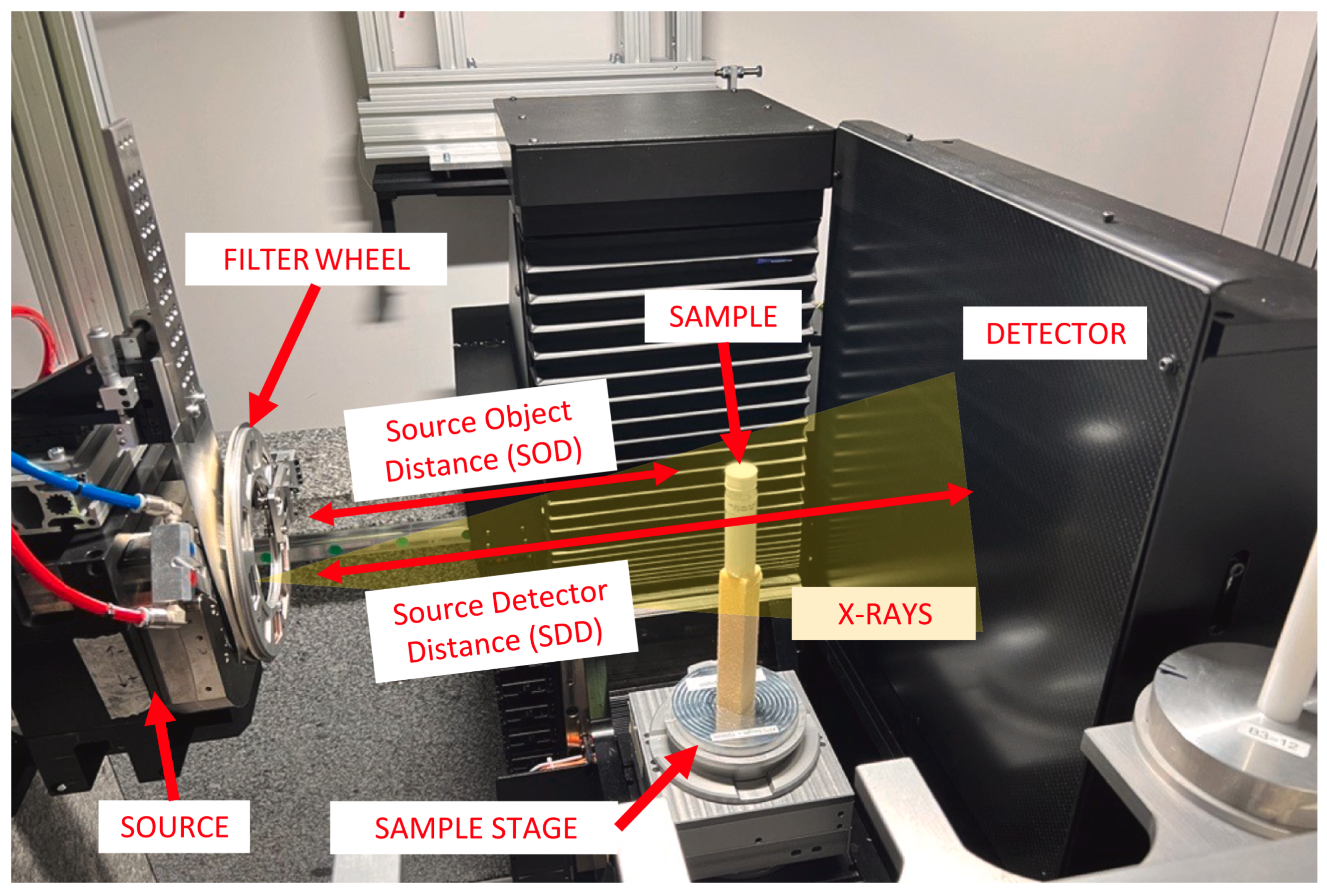
Figure 3.
XCT cross-sections of PCMs exhibiting different morphologies. (a) Solid hexadecane. (b) Solid n- Eicosane. (c) SAT in supercooled state displaying SA crystals and liquid SAT. (d) Mixture of SA and SAT crystals. (e) Incongruent melted CaCl2.6H2O (Stamatiou et al. [70]).
Figure 3.
XCT cross-sections of PCMs exhibiting different morphologies. (a) Solid hexadecane. (b) Solid n- Eicosane. (c) SAT in supercooled state displaying SA crystals and liquid SAT. (d) Mixture of SA and SAT crystals. (e) Incongruent melted CaCl2.6H2O (Stamatiou et al. [70]).
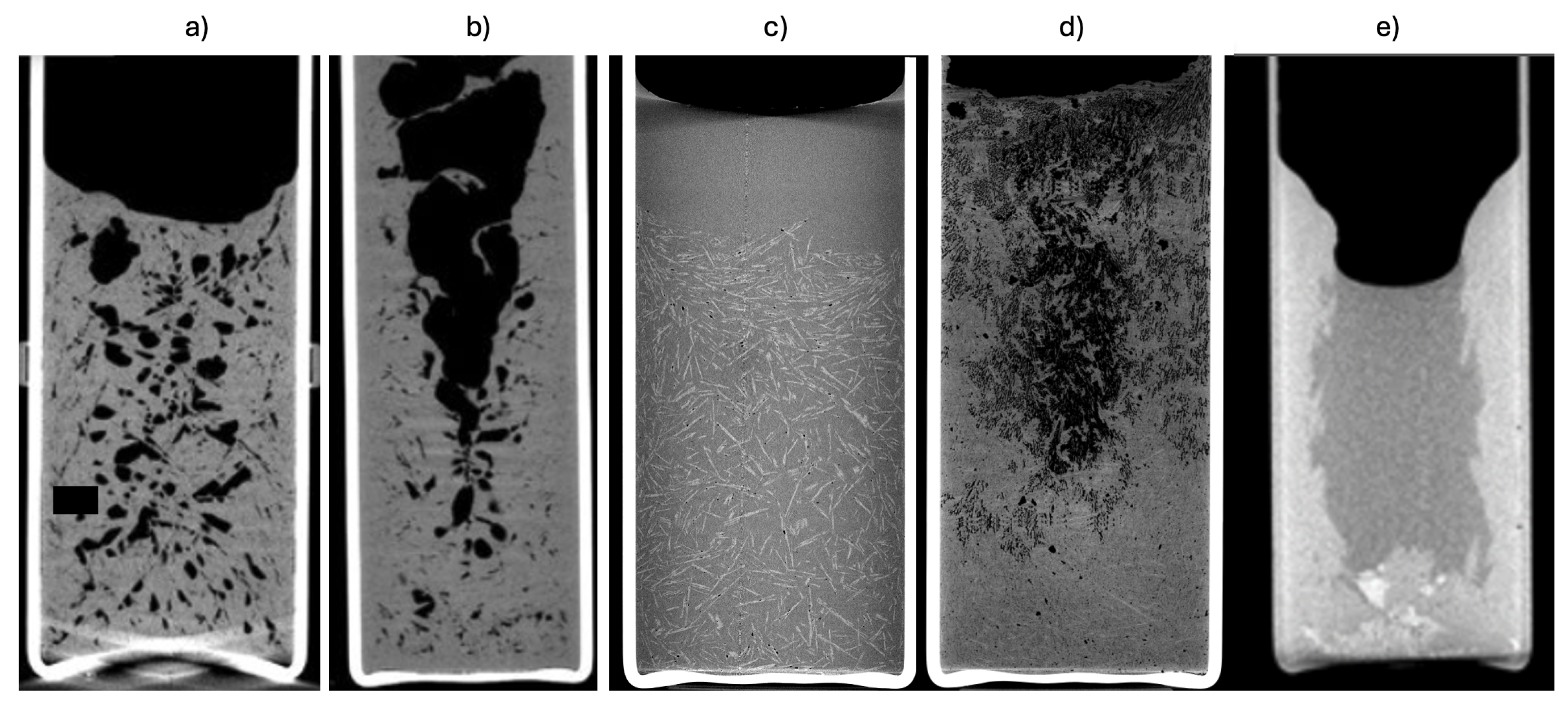
Figure 4.
(a) XCT cross-sections along 3 perpendicular planes and 3D rendering for a SAT PCM sample with minimal supercooling. (b) Same as (a) but for the SAT sample solidified from supercooled state. (Dannemand et. al [68]).
Figure 4.
(a) XCT cross-sections along 3 perpendicular planes and 3D rendering for a SAT PCM sample with minimal supercooling. (b) Same as (a) but for the SAT sample solidified from supercooled state. (Dannemand et. al [68]).
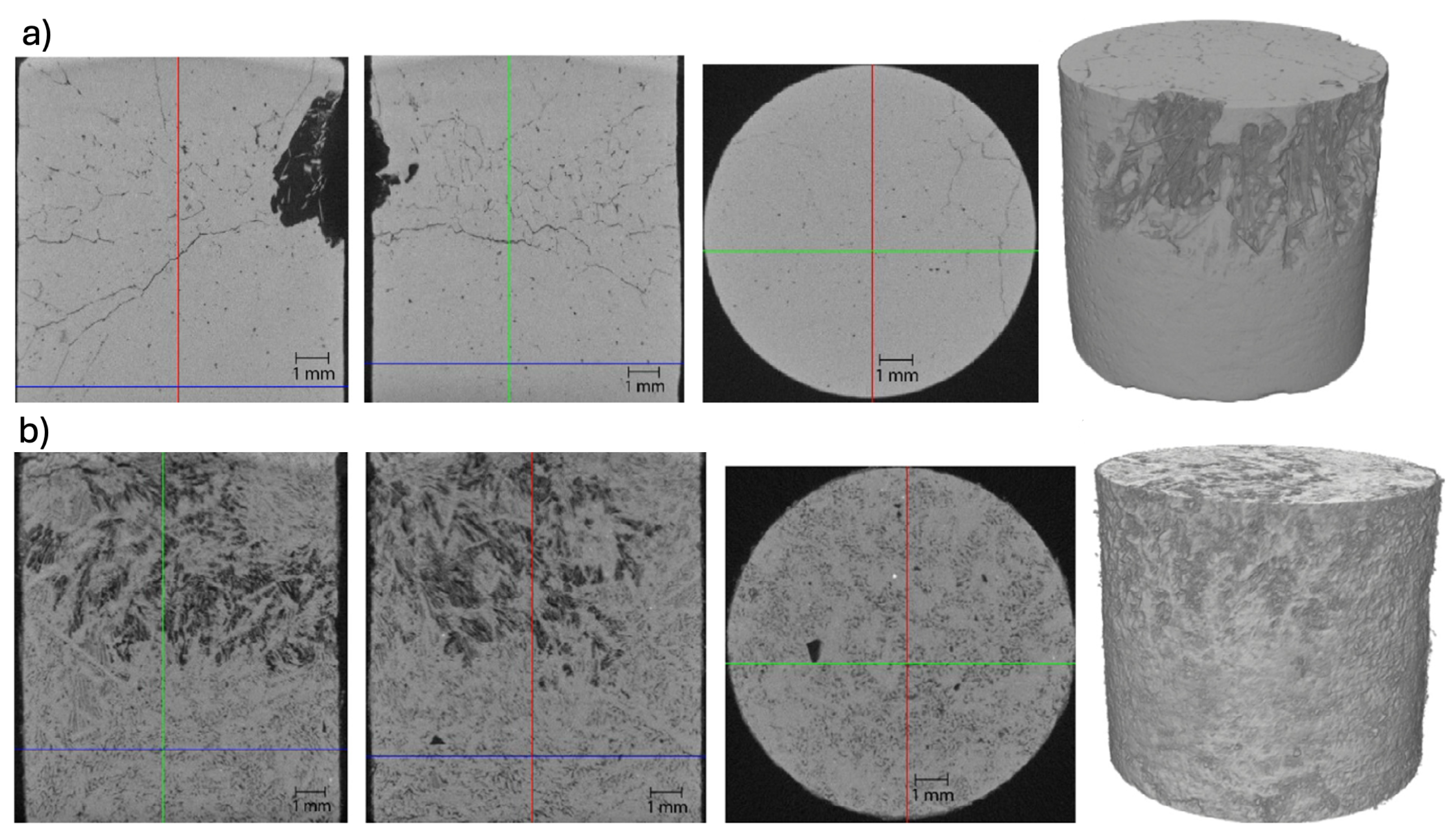
Figure 5.
The appearance of the core-shell NaCl-Al2O3@SiC@Al2O3 macrocapsule after heating at 850°C for 1000 h (a). XCT cross-section images of the NaCl-Al2O3@SiC@Al2O3 macrocapsules at 850 °C 1000 h (b–e). (Liao et. al [73]).
Figure 5.
The appearance of the core-shell NaCl-Al2O3@SiC@Al2O3 macrocapsule after heating at 850°C for 1000 h (a). XCT cross-section images of the NaCl-Al2O3@SiC@Al2O3 macrocapsules at 850 °C 1000 h (b–e). (Liao et. al [73]).
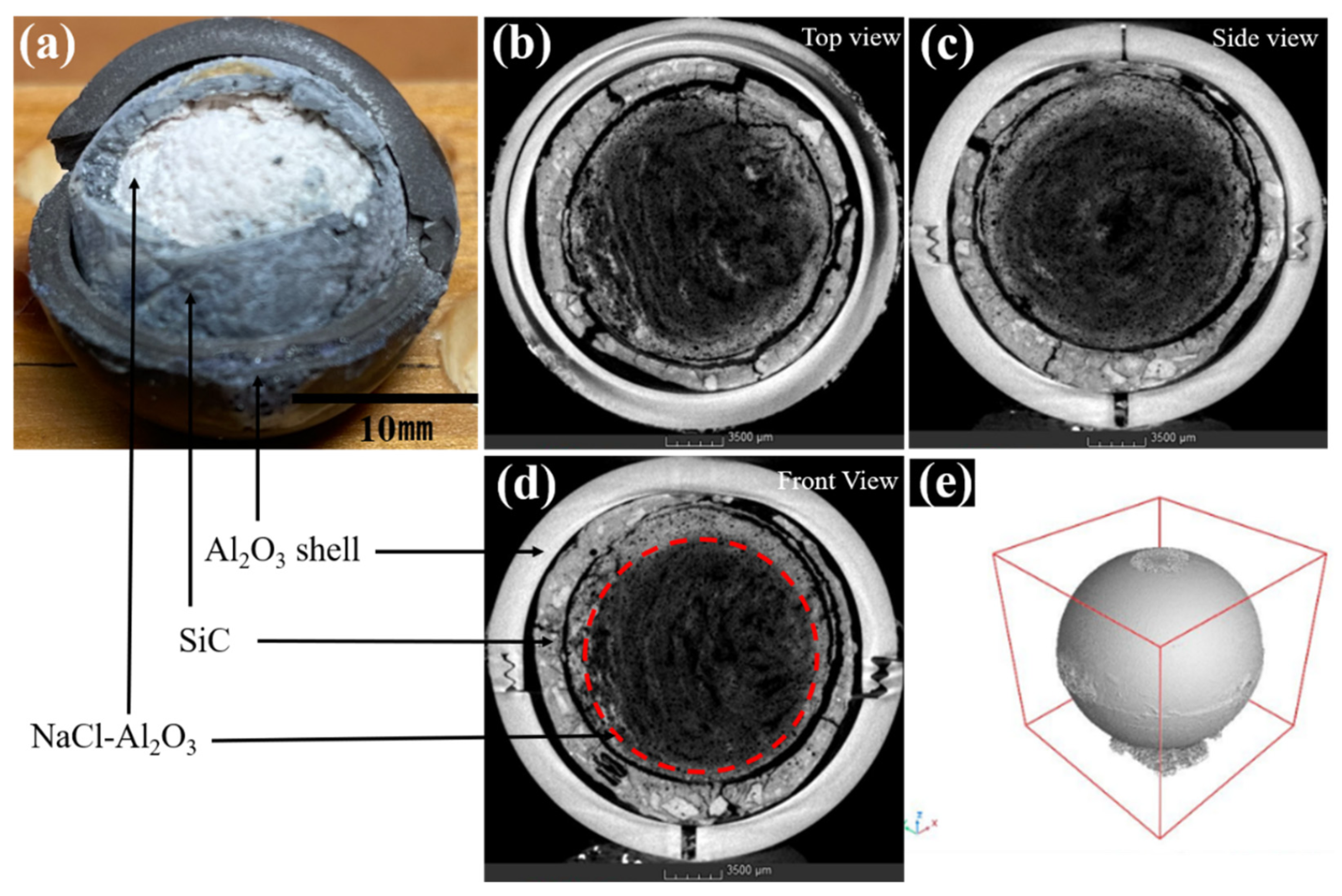
Figure 6.
Temperature profile along the reactor length of three crystallization and melting cycles (a). Mean melting and crystallization temperatures for three cycles(b). Comparison of temperature profile of thermocouple 3 (TC3) with the images from the XCT measurements for the melting process (c). Comparison of the temperature profile (TC4) with the images from XCT measurements in the crystallization process (d). Bright and dark greyvalues denote to solid PCM and liquid PCM, respectively (Kohler et al.[59]).
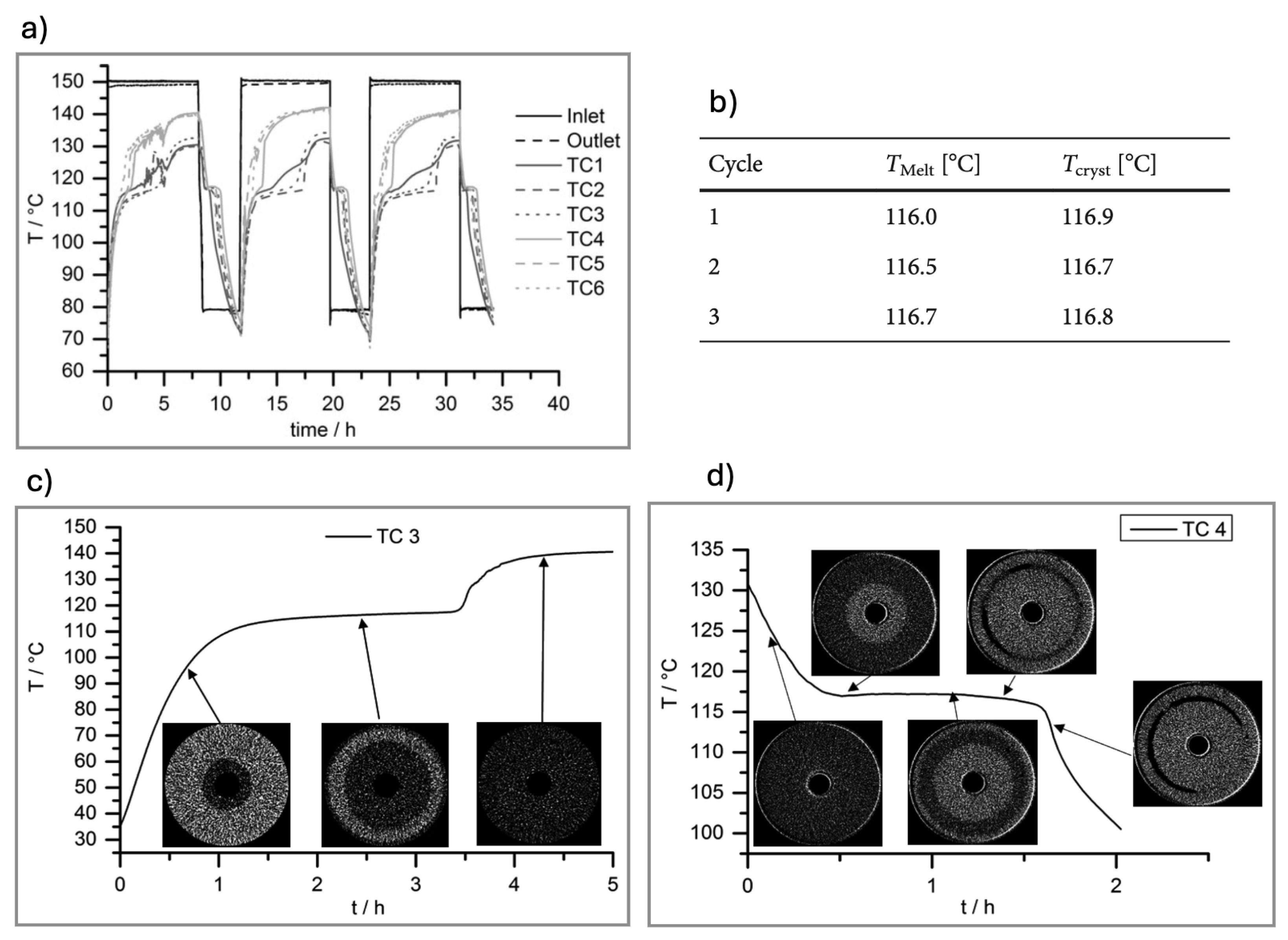
Figure 7.
(a) Evolution of solidification process of CaCl2.6H2O visualised based on the same cross-section of the sample taken at different points in time. (b) Semi-transparent 3D rendering of the crystal formation (grey regions) in CaCl2.6H2O at different times. (c) Transient liquid volume fraction curves for CaCl2.6H2O PCM computed considering (label ‘‘with shrinkage’’) and neglecting volumetric shrinkage (label ‘‘without shrinkage’’). (d) Size of the biggest crystal localised at the bottom surface of the sample as function of time (Martinez-Garcia et al. [61,62]).
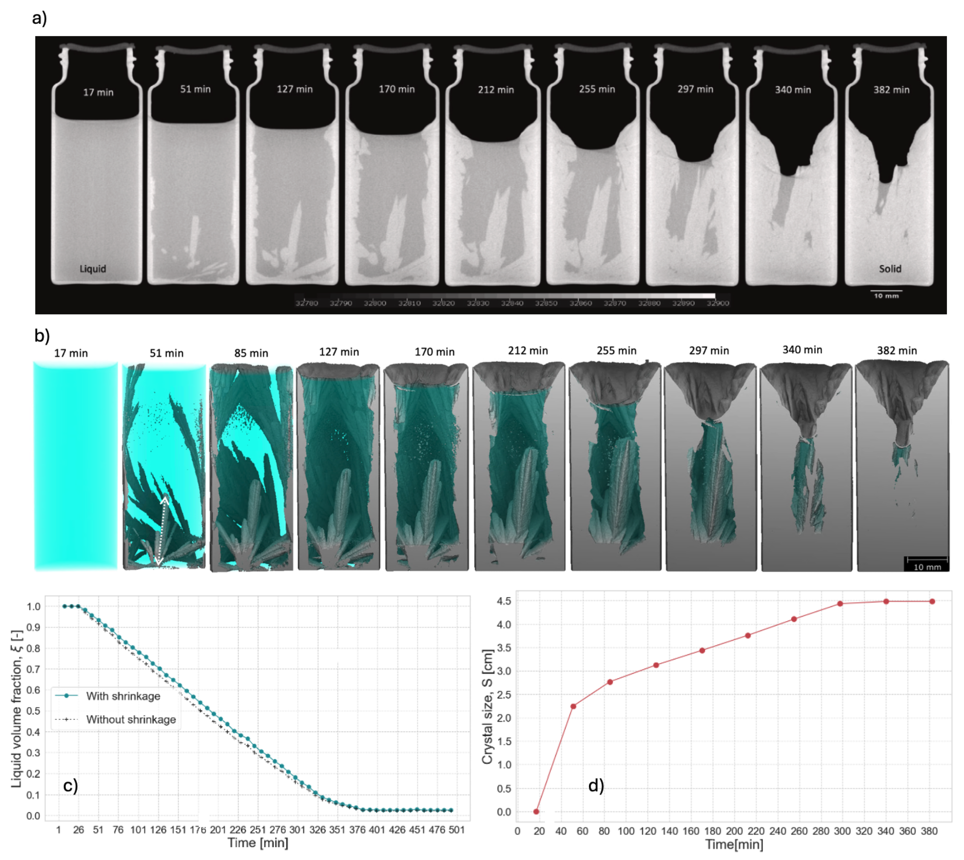
Figure 8.
(a) XCT cross-section sequence for the three repeatability time-lapse XCT experiments. (b) Volumetric liquid fraction plotted against the time for all repeatability test considered. (c) Temperature profiles obtained from the four fibre optic sensors, positioned at the outer surface, top, middle and bottom locations of the sample (Guarda et al. [65]).
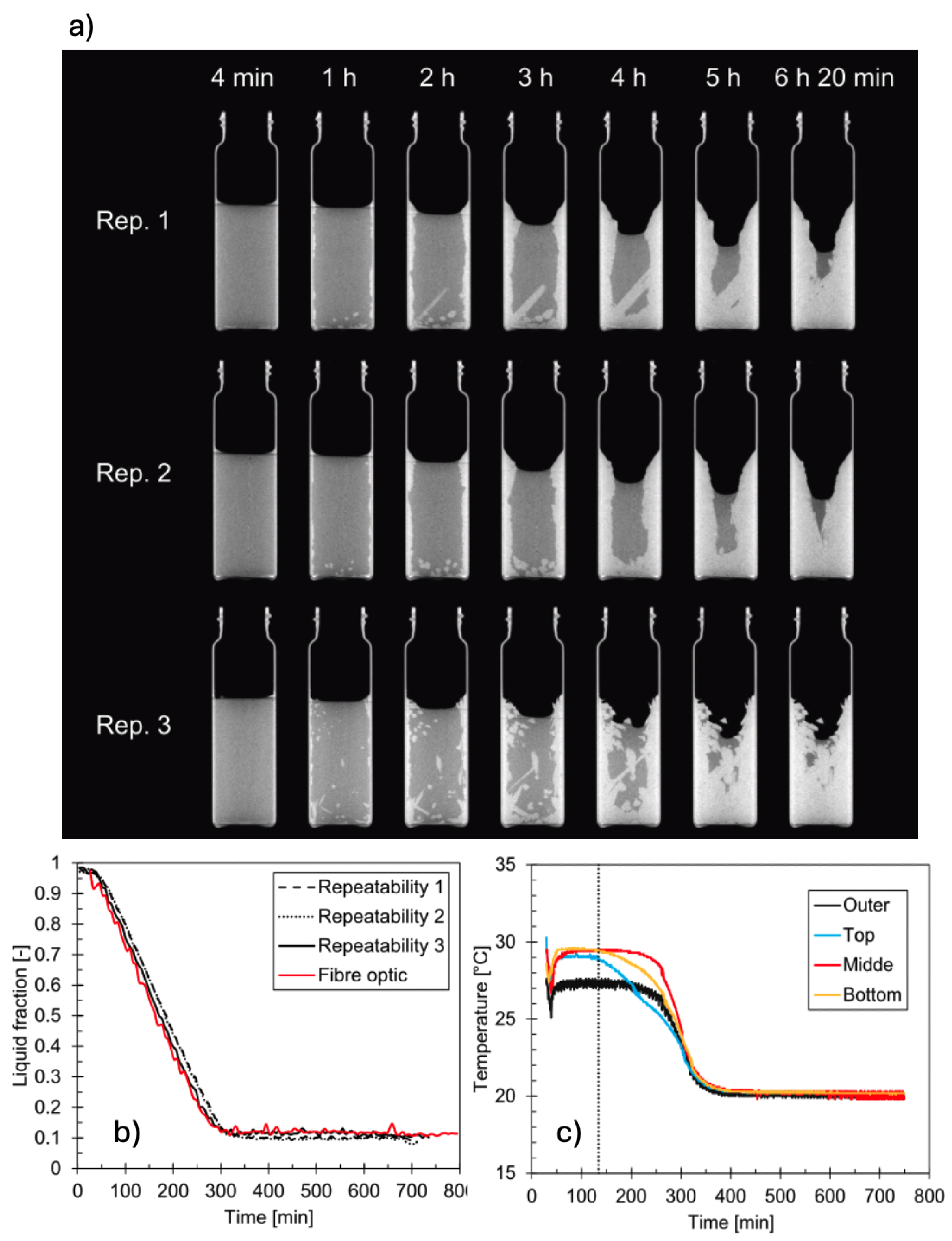
Figure 9.
(a) 3D rendering of XCT images showing the dynamic behaviour of ice melting (ice in brighter grey, water in darker grey colour). (b) Time-dependent liquid volume fraction curve for ice PCM. (c) Nominal actual-comparison maps between the ice-core surfaces extracted at 36 and 56 minutes calculated with the GOM Inspect software (Martinez-Garcia et al. [60,61]).
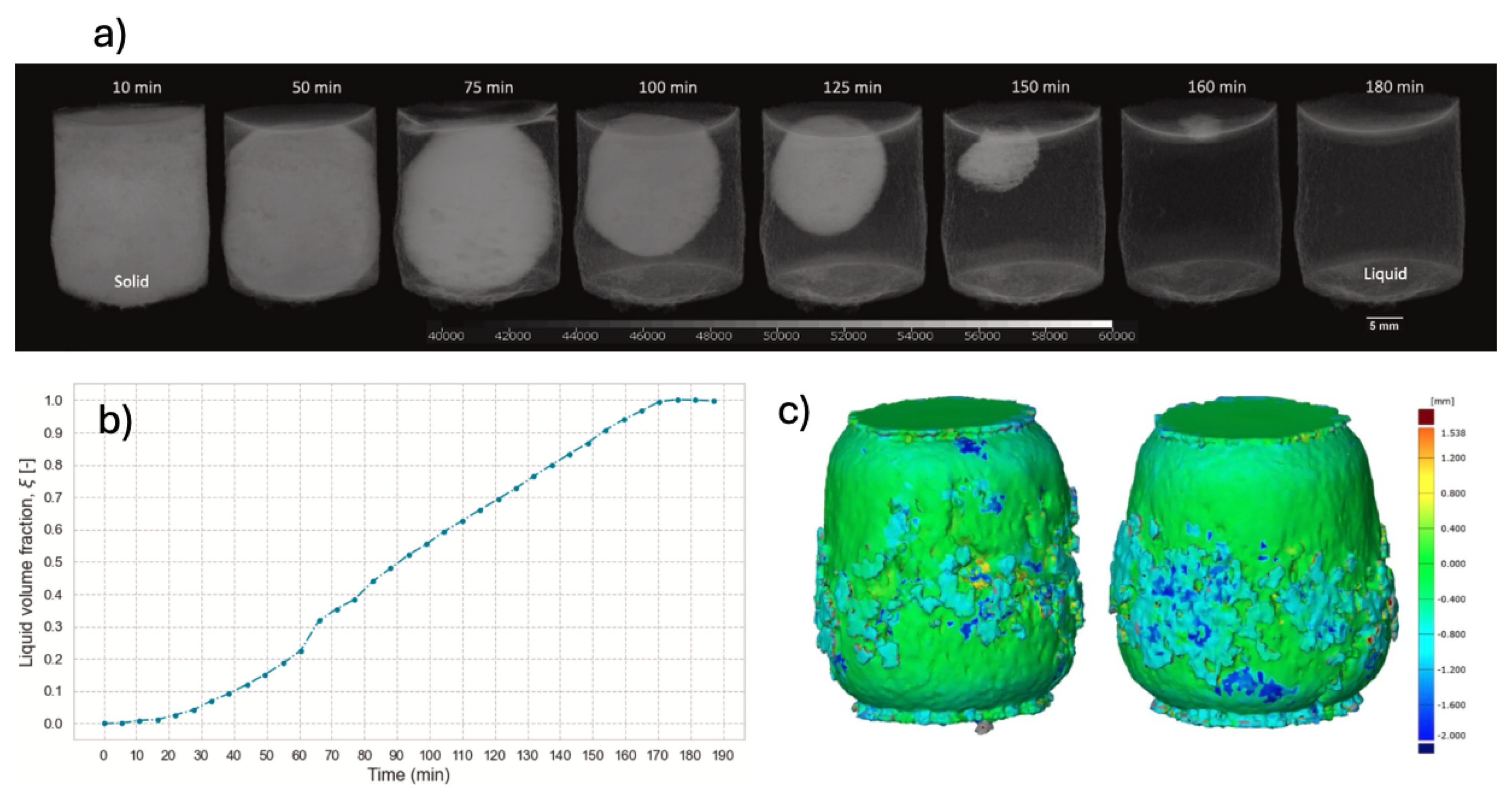
Figure 10.
(a) 3D renderings of the liquid (inner lighter region) and solid (outer nearly transparent region) eicosane phases along its solidification process.). (b) Experimental-numerical comparison for liquid fraction evolution. (c) Vertical cross sections of the sample volume at the beginning (left) and at the end (right) of the XCT experiment are highlighted from the 3D rendering. (Guarda et al. [64]).
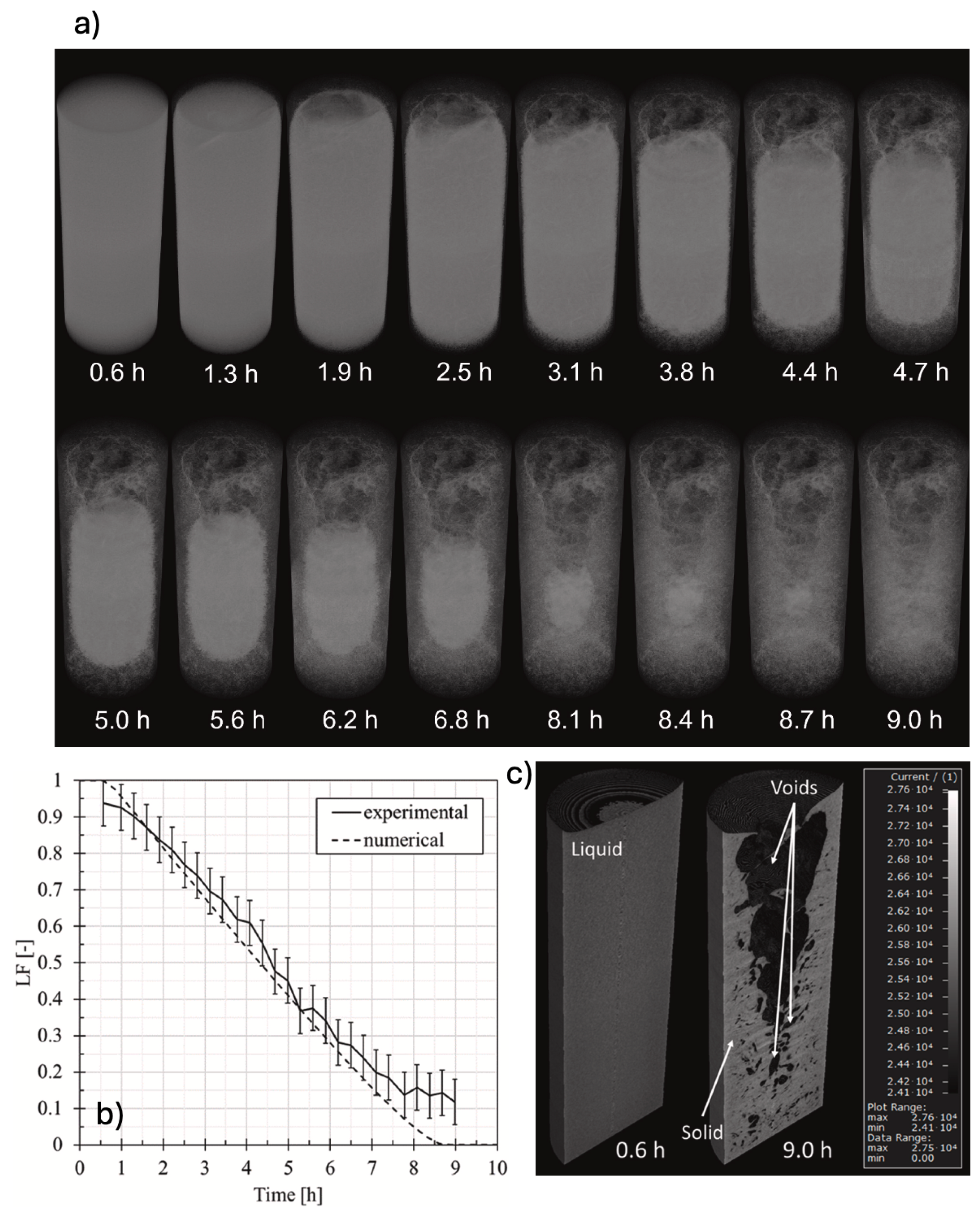
Figure 11.
Results of the optimised model in terms of (a) average temperature of the ice/water system and (b) liquid fraction (LF). Liquid fraction contours comparison (experimental vs numerical). Blue color corresponds to ice, red to liquified zone and others intermediate colors to the mushy region (Guarda et al. [63]).
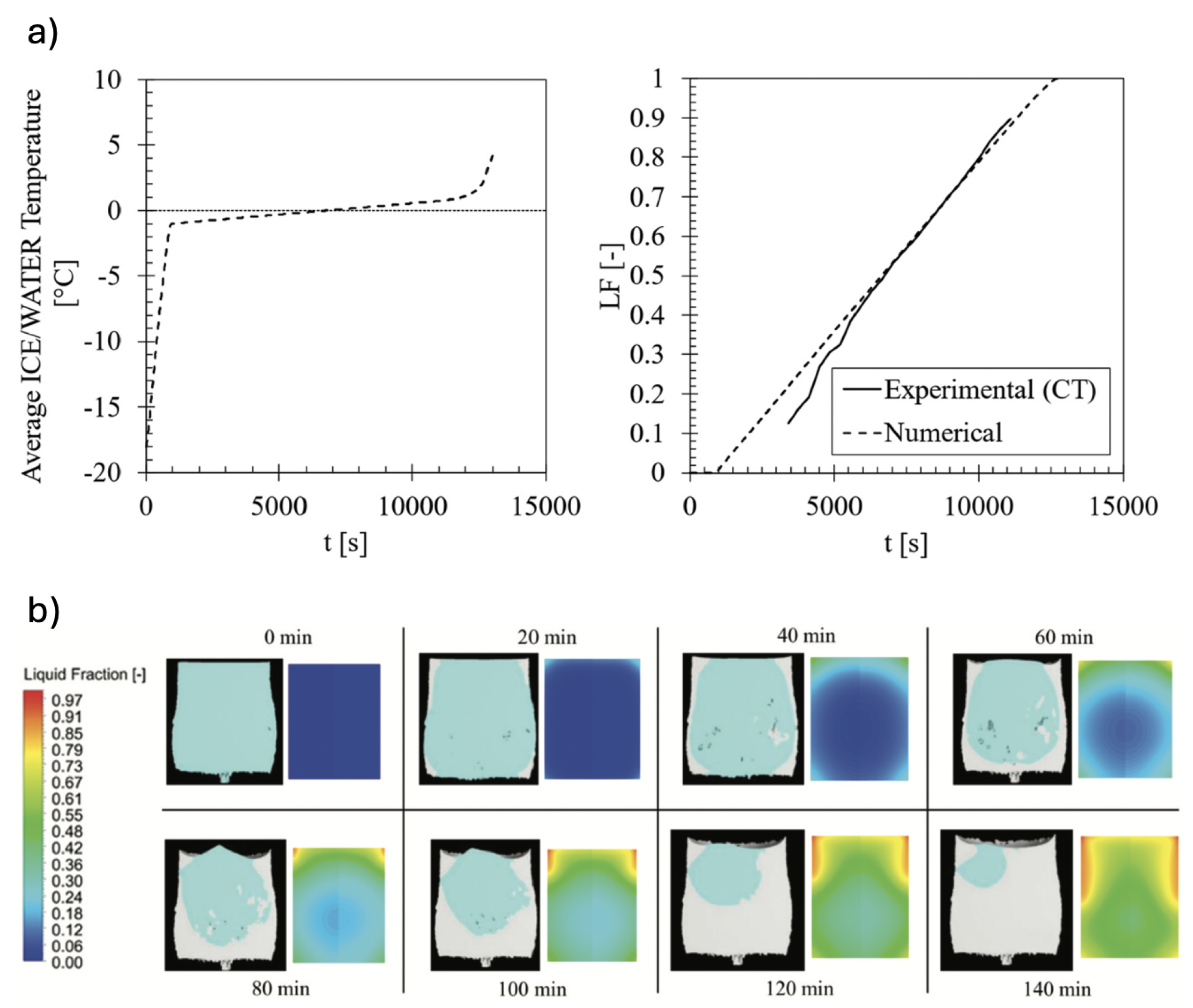
Figure 12.
Synchronous volumetric liquid fraction (black, left axis) and average PCM temperature (red, right axis) (b) coupled to the visualisation of the phase change process during the supercooling (a). Validation of the model on volumetric liquid fraction (c) and average temperature of the CaCl2.6H2O PCM (d) (Guarda et al. [65]).
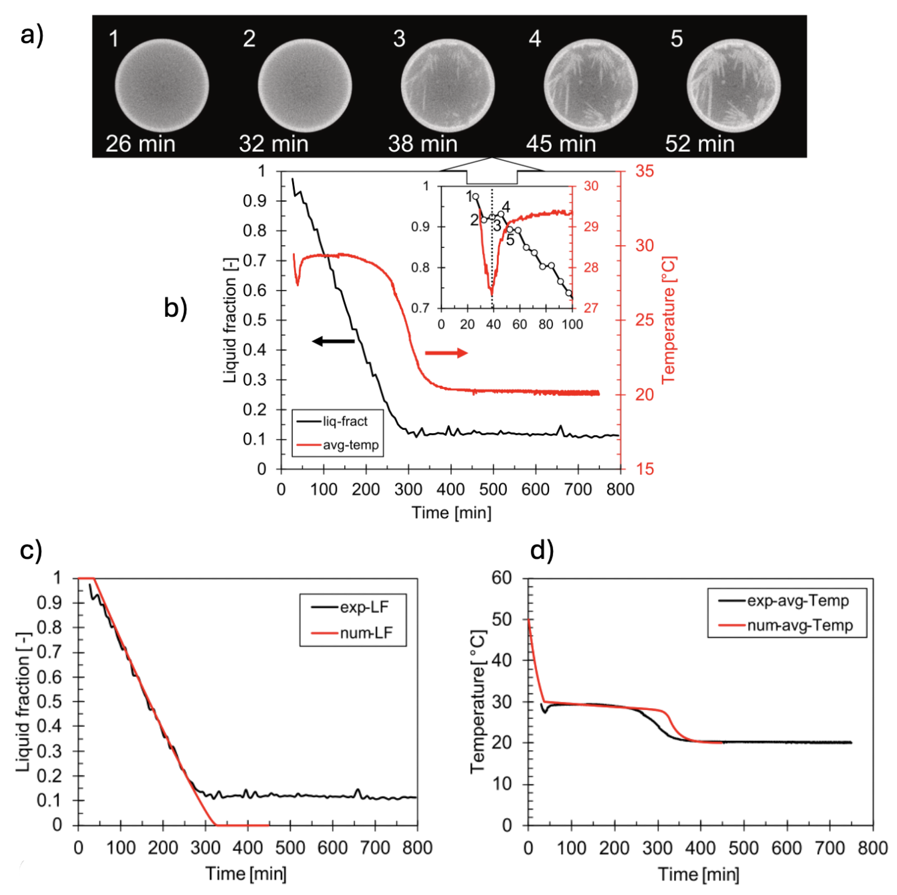
Figure 13.
XCT cross-sections and CFD liquid fraction contours comparison (Guarda et al. [65]).
Figure 13.
XCT cross-sections and CFD liquid fraction contours comparison (Guarda et al. [65]).
Disclaimer/Publisher’s Note: The statements, opinions and data contained in all publications are solely those of the individual author(s) and contributor(s) and not of MDPI and/or the editor(s). MDPI and/or the editor(s) disclaim responsibility for any injury to people or property resulting from any ideas, methods, instructions or products referred to in the content. |
© 2025 by the authors. Licensee MDPI, Basel, Switzerland. This article is an open access article distributed under the terms and conditions of the Creative Commons Attribution (CC BY) license (http://creativecommons.org/licenses/by/4.0/).
Copyright: This open access article is published under a Creative Commons CC BY 4.0 license, which permit the free download, distribution, and reuse, provided that the author and preprint are cited in any reuse.


