Submitted:
02 July 2025
Posted:
04 July 2025
You are already at the latest version
Abstract
Despite efforts to select optimal habitat patches for reintroduction programs, animals released to the wild rarely stay within such designated spots. Therefore, it is important to be able to evaluate their true landscape affiliation. Wisents upon having been reintroduced to the Bieszczady Mountains, have remained in two isolated subpopulations of slightly different habitats. Using movement data obtained through radio-tracking and employing machine learning (ML) techniques (notably, eXtreme Gradient Boosting (XGBoost)) for classification purposes, we were able to obtain a precise determination of preferred habitats within their home rangeswe analyzed 31,480 location records of wisent presence in the Bieszczady Mountains during the years 2002-2021 and correlated this data on land use and land cover obtained from the CORINE Land Cover (CLC) inventory. The machine-learning algorithm XGBoost was then applied to identify the affiliation of individual wisents to habitats within the home range of the given subpopulation. The results showed very high classification performance, with a recognition accuracy of 92% in the vegetative and 96% in the winter seasons. We thus propose a new approach to recognizing the affiliation of particular individuals to their home ranges. This amay considerably improve the decision-making process in conservation and management of wildlife populations.
Keywords:
European bison
; habitat suitability
; XGBoost
; spatial data
; machine learning
; supervised classification
1. Introduction
Wisents/European bison (Bison bonasus L.), after their extirpation from the wild over 100 years ago, were maintained in captivity, and, beginning in 1952, have been gradually reintroduced to certain designated sites that they once naturally occupied. The present world population of the species originates from only 12 founders who survived in captivity, which makes it one of the most inbred mammals in the world [1].
There has been only a few successful reintroductions of this species, all in Central and Eastern Europe, and the newly-established herds have practically remain in isolation from each other. Therefore, the species, due to its very low genetic diversity, is potentially highly threatened by inbreeding depression. This may affect the fitness of individuals, their ability to adapt to changes in environment, and, finally, the chances for long-term survival of the species [2,3,4].
Nevertheless, because of socio-economic problems resulting from damages in agriculture and cultivated forest stands caused by some large wisent herds, it is suggested for the future to maintain rather small populations of wisent within any given area [5,6].
There are two choices regarding the management of small, isolated populations. One is an attempt to establish gene flow, which may lead to outbreeding depression, and the other is to maintain subpopulation isolation , risking inbreeding depression and potential genetic drift [7,8].
Natural exchange of individuals among particular herds is not an easy process be-cause of the general lack of suitable migration corridors for large wildlife species in con-temporary Europe, as well as the social organization of wisent herds, where females with young remain mostly within stationary ranges and only single males are are migratory[9,10].
The reintroduction of wisents to the wild was performed in sites selected according to their known habitat preferences. In some case, however, animals did not remain around the site of the release but moved to other habitat patches or split into separate groups occupying different home range territories [11,12].
Monitoring of spontaneous movements of animals among neighboring herds is very difficult and, in most cases, impossible. Hence, in order to calculate the degree of potential gene exchange, it is important to be able to estimate the intensity of such migrations. That can be achieved by identifying the affinity of particular individuals to their maternal groups.
An earlier attempt to distinguish wisents occupying different home ranges (i.e. be-longing to different herds) during both the vegetative and winter seasons was done through kernel density estimation and spatial analysis. The results obtained using the different methods show that there is a possibility of generalization [13,14].
The advent of modern data collection techniques and geospatial technology including real-time location tools and high-resolution satellite imagery has led to the generation of vast amounts of data. In this regard, machine learning algorithms facilitate their deeper analysis and bring about better understanding of the actual situation. In contrast, classical statistical methods are constrained by numerous limitations and assumptions regarding the type of data and the relationships between variables.
Therefore, in this paper we tested the machine learning approach for spatial data classification, seeing this as a new method for recognizing the affiliation of particular individuals to their maternal home ranges. This approach, we think, could be, useful for future management of free-ranging populations. In this regard, the eXtreme Gradient Boosting (XGBoost) algorithm was applied for classification tasks due to its high efficiency and superior performance in processing large datasets. The present study was primarily concerned with the following: (1) introducing a novel ML approach for subpopulation identification based on animal presence data, (2) developing the XGBoost method for classification by using CLC data, and (3) generating comparative analysis of the classification efficiency of the vegetative and winter seasons.
2. Materials and Methods
2.1. Study Area
The free-ranging wisent herds currently inhabiting the Bieszczady Mountains originate from two reintroductions: the first in 1963 to the eastern part of the range, and the second in 1980 to its western part. All introduced individuals originated from captivity and belonged to the Lowland – Caucasian line, bearing genes of the only representative of Caucasian wisents (the Caucasus #100) that survived in the breeding center. The eastern subpopulation (known as the Tworylne herd) dwells within the forest districts of Lutowiska and Stuposiany and partially within the Bieszczadzki National Park [1,15,16]. The home range of the western subpopulation (known as the Baligród herd) extends over the forest districts of Baligród, Komańcza, Cisna, and Lesko (Figure 1).
During the period of time covered by this study (2002 and 2021), wisent numbers in Bieszczady grew from about 150 to about 700 individuals, which is over 40% more than the target number originally planned for this population [17,18]. Such significant increase of population numbers could be associated with intensified use of the most preferred habitats and overexploitation of natural food base as well as depredation of crops [19, 20}. In this study we analysed data on the occurrence of wisents in habitat patches within the home ranges inhabited in Bieszczady by two subpopulations of this species.
The Bieszczady Mountains, being a part of the Western Carpathians, are situated in southeastern Poland. Their maximal elevation is at 1346 m above sea level, and they are mostly forested (almost 85% of their total land cover). The tree stands are dominated by beech-fir (Fagus sylvatica-Abies alba) associations, with alder-willow (Alnus glutinosa-Salix spp.) woods along watercourses. A considerable part of the presently forested area is also overgrown with Scotch pine (Pinus sylvestris), replanted or originating from secondary succession on former cultivated fields [16]. The majority of home ranges of both subpopulations are forested: for the western subpopulation, the forested area is 593 km2 and the open area is 237 km2, and for the eastern subpopulation, the forested area is 678 km2, and the open area is 183 km2.
2.2. Data Collection
We used for this analysis, 31480 records of wisent presence of two subpopulations: western (the Baligród herd) and eastern (the Tworylne herd) obtained between 2002 and 2021) from 6 radiocollared individuals (3 in every herd). The raw data we employed included telemetric fixes collected by the staff of the Carpathian Wildlife Research Station of the Polish Academy of Sciences (under the framework of the routine monitoring of free-ranging wisent in the Bieszczady Mountains). This survey was undertaken in the vegetative season (between April and October) and the winter season (between November and March). Table 1 shows the wisent presence records of the two subpopulations as broken down to season and in total.
Spatial distribution of free ranging wisent presence during the vegetative and winter seasons is shown in Figure 2 (a), (b).
The available set of telemetric data for every record consisted of the date and hour, elevation above sea level (a.s.l. [m]), and the location of the animal in WGS84 projection. Geospatial data were added to the numerical map of the Bieszczady Mountains via ArcGIS software. Next, thematic layers were created for further analysis (forested area, open land, composition of tree stands, infrastructure, elevation above sea level, records of wisent presence), which allowed for identifying their mutual relationships. Habitat parameters within both wisent ranges were classified according to CLC regulations. This land cover and land use inventory consists of 44 thematic classes, including forests, agricultural land, and human-related infrastructure [18]. Analyses were performed for three levels of CLC (Table 2, Table 3, Table 4, Table 5, Table 6, Table 7 and Table 8).
At the time of data collection, the average elevation above sea level was different within the home ranges of both subpopulations (Table 2).
The western subpopulation was found to inhabit generally higher elevations, by about 90 m on average. During the vegetative season, this difference was much lower – about 61 m, but in winter – it was over 118 m. Seasonal differences were much higher (about 83 m) within the area occupied by the eastern subpopulation, while between seasonal home ranges of the western subpopulation, elevation differed by only about 26 m.
On average, land cover and land use within the home ranges of both subpopulations were quite similar, with forests covering above 90% of their area, with much lower percentages of cultivated land being occupied (Table 3 and Table 4). The pertinent percentages are highlighted in bold text.
During the vegetative season, the home range of the eastern subpopulation contained more open spaces (by little over 4%), while that of the western population demonstrated more forested area occupation (by about 5%). During the winter season, the proportion of forests and open land was almost identical.
Types of land use and land cover within the home ranges of the Baligród and Tworylne herds according to CLC level 2 classification are presented in Table 5 and 6.
A comparison of the home ranges of both subpopulations according to CLC level 2 classification reveals that the percentage of forest inhabitation differed by about 7% during the vegetative season for the western subpopulation, in contrast to the eastern population. In the home range of the eastern subpopulation, however, the percentage of pastures and arable land habitation was greater during the vegetative season by about 2%, in contrast to the western population (Table 5). During the winter season, the differences between home ranges of both subpopulations were very slight, not exceeding 1%.
The analysis undertaken for CLC level 3 (Table 7 and Table 8) with regard to types of forest stands found in each subpopulation home range shows significant differences. Within the home range of the western subpopulation, coniferous stands were much more frequently evident (over 24% difference), while mixed forests were significantly less notable (by almost 16%). Moreover, the share of broad-leaved stands, was lower by about 7% within the home range of the western subpopulation (Table 7).
The aforementioned data demonstrates that the only significant differences between the home ranges of both wisent subpopulations lies in the proportions of various types of tree stands, mainly in the vegetative season (by about 35% higher for coniferous forest for the western subpopulation and 23% for mixed forest for the eastern subpopulation). Proportions of forest cover and open lands are, however, quite similar.
2.3. Extreme Gradient Boosting Algorithm
The XGBoost algorithm was created by Tiangi Chen and Carlos Gusterin in 2016 [21]. XGBoost combines a number of weak classifiers into a single strong classifier using the gradient tree boosting technique [22,23,24].
Let where and be a given data set with examples and features. A tree ensemble model using base models to predict the result can then be written in the form [21]:
where is the final tree model, is the previous tree model and is the newly generated tree model.
The process of learning the model estimates the model parameters by minimizing the objective function [21]:
where is the prediction of the target , is the training loss and represents the regularization term.
By substituting the formula (1) into (2) and simplifying the formula (2) the objective function can be transformed into the following form:
where functions and are the first and second order gradient statistics of . Moreover, the regularization term , can be written in the form:
where parameters and are penalty coefficients, and the number is the total number of tree leaves.
The solution of (3) gives the optimal weight of leaf [21]:
where denotes the instance set of leaf .
2.4. Logistic Regression
The logistic regression model for the dichotomous variable with values 0 and 1 is defined by the formula:
where for are the regression coefficients and are the independent variables. To predict a class for , the probability is compared to a classification threshold, which is usually equal to 0.5.
2.5. Evaluation Metrics
In binary classification, only two classes are considered: one of which is usually referred to as 'positive' and the other as 'negative'. The number of correct classifications, represented by true positives (TP) and true negatives (TN), and the number of misclassifications, represented by false positives (FP) and false negatives (FN), are illustrated in Figure 3 [27]. The "Actual Class" refers to the true, correct label of a data point in a classification problem. It is the "ground truth" or the known correct classification.
The following indicators are used:
- Accuracy – the percentage of correct classifications:
- 2.
- Precision – the number of cases, expressed as a percentage, in which the classifier yielded the correct result:
- 3.
- Recall (sensitivity, true positive rate) – the ability of the model to capture positive cases:
- 4.
- Specificity (true negative rate) – the ability of the model to capture negative cases:
- 5.
- F1-score – the harmonic mean of precision and recall:
- 6.
- Receiver Operating Characteristic (ROC) curve – a visual representation of the relationship between the efficiency of classifying positive cases (sensitivity) and the inefficiency of classifying negative cases (1 – specificity) using all possible classification thresholds. The area under the perfect ROC curve (AUC) is equal to 1 [27].
2.6. Model Development
In our research, the XGBoost algorithm from the xgboost Python package [28] was employed to identify the affiliation of an individual with its proper subpopulation. Afterwards, a grid search method was applied to find the best XGBoost classification model. The entire machine learning modelling can be described thusly:
The geospatial data was processed via ArcGIS packages to create tabular data.
The tabular data was preprocessed in order to choose the proper variables and eliminate missing or incorrect values.
The final data set was divided into training and test subsets by applying the 80:20 rule.
A randomized search model was applied so as to reveal the most suitable hyperparameters. Here, 40 sets of random hyperparameters were selected from the grid search by applying cross-validation splitting strategies [28,29]. The optimal values of hyperparameters were then found based on the AUC ROC metric, through partitioning of the training data into 10 subsets. Finally, the best set of parameters found in the grid was returned so as to uncover the best estimator.
The optimized XGBoost model was employed to make predictions for training and test sets. Next, the evaluation metrics were calculated and compared.
3. Results
In the presented work, we applied the powerful machine learning algorithm XGBoost. The XGBoost model was compared to the logistic regression model, as the latter is a baseline binary classification algorithm.
3.1. Model Settings
The data used in the classification procedure included 17,737 records of wisent presence during the vegetative season and 13,743 records during the winter season.
The data contains the class variable describing the wisent subpopulation (Baligród herd – 0, Tworylne herd – 1), and four feature variables: the numeric variable elevation a.s.l. [m] and three categorical variables including thematic classes of the CLC level 1, CLC level 2 and CLC level 3 data. The conducted analysis was done for each season separately. The XGBoost model was optimized based on grid search parameter tuning with 10-fold cross-validation. The optimal hyperparameters values of the XGBoost model are presented in Table 9.
Figure 4 (a) and (b) illustrates the training and test curves of the developed XGBoost model for both vegetative and winter seasons.
The stable shape and descending trend of these curves clearly evident the correctness of the developed XGBoost behaviour. Accordingly, the training loss was reduced to less than 0.1. The test loss is, however, slightly greater than the training loss. Still, XGBoost avoided overfitting during the training process.
3.2. Model Performance
The evaluation metrics used to describe the performance of the optimized XGBoost model for the vegetative and winter seasons are presented in Table 10.
We can observed that the XGBoost model achieved very high performance metrics for both seasons, although they were higher for the winter season. Furthermore, all metrics achieved very high results for both the training and test sets. Here, the accuracy values were around 91% for the vegetative season and 96% for the winter season. It can also be noted that the F1-score values were around 85% and the ROC-AUC values were around 90%. Such results correspond to very high model classification efficiency. This is also confirmed by high values of precision, recall and specificity, the highest of which are specificity values. These values reveal that the model very successfully classified individuals belonging to the Tworylne herd. The confusion matrices of the XGBoost classifier for the vegetative and winter seasons based on the independent test sets are shown in Table 11 and 12. The best results are in bold font.
In addition, the performance of the XGBoost model was compared with the performance of a baseline model for binary classification tasks (logistic regression) using the same training and test datasets. For comparison, the evaluation metrics for logistic regression are shown in Table 13.
The ROC-AUC values for the vegetative season based on the training and test sets were very low, about 55%. In the case of the winter season, these values were slightly better (about 65%). The results showed that the quality of the classification was very low, especially during the vegetative season. We can also observe that XGBoost achieved significantly higher values for all evaluation metrics except specificity, demonstrating the superiority of this method.
4. Discussion
In contemporary Europe, wildlife species mostly occupy relatively small, isolated patches of suitable habitats. Moreover, ecological connectivity among such sites often does not exist due to considerable fragmentation of the environment and numerous man-made barriers such as industrial or transportation infrastructure, settlements, etc. The size of the remaining fragments of natural habitats is often too small to support viable populations. Therefore, subpopulations of wildlife species are frequently threatened by inbred and loss of genetic diversity, which finally may lead to their extinction [31,32,33,34].
A solution to this problem is the restoration of ecological corridors, and doing so will allow the spontaneous exchange of individuals through migrations. This will enable their occupying suitable habitat patches outside of maternal home ranges [35]. Unfortunately, the assessment of the intensity of such natural processes is very difficult and often impossible unless there is a sufficient number of animals being radio-collared or permanently marked, thus enabling identification of their origin. This, however, requires complicated and expensive procedures connected with capturing, immobilization, and further monitoring of a sizable group of individuals [36].
Therefore, other methods that make it possible to distinguish individuals of different derivations provide valuable assistance in the conservation and management of wildlife species. The application of the XGBoost algorithm, in enabling the classification of particular animals as native to a given home range of a herd indicating its actual habitat preferences, provides such an opportunity.
Earlier, such attempts were based upon the use of kernel density estimation and spatial analysis. Unfortunately, the obtained products did not prove the universality of those approaches. Indeed, the results of applying such models to the available data pertaining to different herds varied considerably in their quality [13,14]. Although ranges inhabited by both herds had similar percentage of forested area, their stand compositions were quite different. In both cases, the most intensively used parts of their home ranges were situated more than 10 km from the respective sites of release. Such situation reflects the ability of wisents to select optimal habitat patches [17}.
Regarding the limitations of our study, we investigated only two herds of wisents. This is because datasets on the spatial distribution and habitat use of these two herds are quite extensive. In contrast, the monitoring of neighbouring herds in Slovakia and Ukraine has been much less intensive and has been carried out over shorter periods of time.
Moreover, differences in habitat selection could result not only from local availability of habitat patches, but to a certain extent, from variation in genetic or physiological traits, since the animals used for introductions were obtained from various breeding centres of diverse conditions.
In this study, we compared the classification results to one traditional model – logistic regression. However, the main aim of our study was to develop the XGBoost algorithm for the classification task. Further research will focus on using a larger dataset and on applying different machine learning models.
Nevertheless, the obtained results confirm the usefulness of the applied tool for analyses of the spatial structure of wildlife populations and for the facilitation of selection of optimal habitat patches for introductions of wildlife species.
5. Conclusions
In our study, the powerful machine learning XGBoost model was developed and applied for wisent herd classification as based on CLC data. The proposed optimized XGBoost model was shown to be an effective method for recognizing individual affiliation to habitats within a home range of a given subpopulation. Our experiments, based on grid search parameter tuning revealed that the examined model provided very high performance metrics for both the vegetative season (accuracy of 91.63%, F1-score of 85.81% and ROC-AUC of 89.05% for the test set) and winter season (accuracy of 96.01%, F1-score of 84.64% and ROC-AUC of 89.34% for the test set). These demonstrate that if there is available a considerable set of telemetric data, the ML approach may provide very accurate identification of habitat patches preferred by animals within their home ranges, so therefore it can be truly useful in the decision-making process for the management of wisents, as well as for other wildlife populations.
Author Contributions
conceptualization, methodology, software, writing – original draft preparation, writing – reviewing and editing, Małgorzata Charytanowicz, Kajetan Perzanowski; visualization, investigation, data curation, Maciej Januszczak, Maria Sobczuk, Aleksandra Wołoszyn-Gałęza; software, validation, Maciej Januszczak, Maria Sobczuk; analysis and interpretation of results, Małgorzata Charytanowicz, Kajetan Perzanowski; methodology, formal analysis, Piotr Kulczycki; supervision, project administration, Kajetan Perzanowski. All authors have read and agreed to the published version of the manuscript.
Funding
This research received no external funding.
Data Availability Statement
Available from the corresponding author after a reasonable request.
Acknowledgments
Data for this study was gathered during the program for continuous monitoring of European bison at Bieszczady, supported by the Regional Directorate of State Forests of Krosno. Authors kindly thank Mr Jack Dunster for linguistic improvement of the text.
Conflicts of Interest
The authors declare no conflict of interest.
References
- Krasińska, M. , Krasiński, Z., Olech, W., Perzanowski, K. European bison. In Meletti, M., Burton, J. (Eds.), Ecology, evolution and behaviour of wild cattle: Implications for conservation. Cambridge University Press, 2014, pp. 115–173.
- Saccheri, I. , Kuussaari, M., Kankare, M., Vikman, P., Fortelius, W., Hanski, I. Inbreeding and extinction in a butterfly metapopulation. Nature 1998, 392, 491-494. [Google Scholar] [CrossRef]
- Weeks, A.R. , Stoklosa, J., Hoffmann, A.A. Conservation of genetic uniqueness of populations may increase extinction likelihood of endangered species: The case of Australian mammals. Frontiers in Zoology 2016, 13, 31. [Google Scholar] [CrossRef] [PubMed]
- Ralls, K. , Ballou, J.D., Dudash, M.R., Eldridge, M.D.B., Fenster, C., Lacy, R.C., Sunnucks, P., Frankham, R. Call for a paradigm shift in the genetic management of fragmented populations. Conservation Letters 2018, 11, e12412. [Google Scholar] [CrossRef]
- Perzanowski, K. , Blehyl, B., Olech, W., Kuemmerle, T. Connectivity or isolation? identifying reintroduction sites for multiple conservation objectives for wisents in Poland. Animal Conservation 2019, 23, 212–221. [Google Scholar] [CrossRef]
- Olech, W. , Perzanowski, K. European Bison (Bison bonasus) Strategic Species Status Review 2020. IUCN SSC Bison Specialist Group; European Bison Conservation Center, 2022. https://www.iucn.org/commissions/ssc-groups/mammals/ mammals-a-e/bison.
- Crandall, K.A. , Bininda-Emonds, O.R.P., Mace, G.M., Wayne, R.K. Considering evolutionary processes in conservation biology. Trends in Ecology & Evolution 2000, 15, 290–295. [Google Scholar] [CrossRef]
- Liddell, E. , Carly, A.B., Cook, N., Sunnucks, P. Evaluating the use of risk assessment frameworks in the identification of population units for biodiversity conservation. Wildlife Research 2020, 47, 208–216. [Google Scholar] [CrossRef]
- Ziółkowska, E. , Perzanowski, K., Bleyhl, B., Ostapowicz, K., Kuemmerle, T. Understanding unexpected reintroduction outcomes: Why are not European bison colonizing suitable habitat in the Carpathians? Biological Conservation 2016, 195, 106–117. [Google Scholar] [CrossRef]
- Bluhm, H.T. , Engleder, T., Heising, K., Janik, T., Jirku, M., Konig, H.J., Kowalczyk, R., Kuijper, D., Maslanko, W., Michler, F., Neumann, E., Oeser, J., Olech, W., Perzanowski, K., Ratkiewicz, M., Romportl, D., Šálek, M., […], Kuemmerle, T. Widespread habitat for Europe’s largest herbivores, but poor connectivity limits recolonization. Diversity and Distributions 2023, 29, 423–437. [Google Scholar] [CrossRef]
- Perzanowski, K. , Januszczak M., Wołoszyn-Gałęza A. Group stability – a pilot study of a wisent herd of Bieszczady Mountains. European Bison Conservation Newsletter 2015, 8, 33–40. [Google Scholar]
- Wasiak, P. , Perzanowski K. Post-release dispersal patterns of wisent bulls introduced to Bieszczady Mountains. European Bison Conservation Newsletter 2014, 7, 115–120. [Google Scholar]
- Charytanowicz, M. , Perzanowski, K., Januszczak, M., Woloszyn-Galeza, A., Kulczycki, P. Application of Complete Gradient Clustering Algorithm for analysis of wildlife spatial distribution. Ecological Indicators 2020, 113, 106216. [Google Scholar] [CrossRef]
- Charytanowicz, M. , Perzanowski, K., Januszczak, M., Woloszyn-Galeza, A., Kulczycki, P. Habitat suitability for wisents in the Carpathians – a model based on presence only data. Ecological Informatics 2022, 69, 101626. [Google Scholar] [CrossRef]
- RDLP. Regionalna Dyrekcja Lasów Państwowych w Krośnie (The Regional Directorate of State Forests in Krosno) [Last accessed 16 November 2024]. https://www.krosno.lasy.gov.pl.
- Marszałek, E., Perzanowski, K. Żubry z krainy polonin/Wisents from the land of poloniny. Ruthenus, Krosno, 2018.
- Perzanowski, K. Żubr w Bieszczadach – stan i perspektywy populacji (Wisent in Bieszczady Mountains – status and perspectives of the population. In: Górecki, A., Zemanek, B. (Eds.), Bieszczadzki Park Narodowy – 40 lat ochrony, 2016, pp. 329–337. BdPN, Ustrzyki Górne.
- Copernicus. Corine land cover [Last accessed 16 November 2024]. https://land.copernicus.eu/en/products/ corine-land-cover.
- Klich, D. , Łopucki, R. , Perlińska-Teresiak, M., Lenkiewicz-Bardzińska, A., Olech, W., Human–Wildlife Conflict: The Human Dimension of European Bison Conservation in the Bieszczady Mountains (Poland). Animals 2021, 11, 503. [Google Scholar]
- Sobczuk, M. , Olech, W. , 2016. Damage to the crops inflicted by European bison living in the Knyszyn Forest. European Bison Conservation Newsletter 2016, 9, 39–48. [Google Scholar]
- Chen, T. , Guestrin, C. Xgboost: A Scalable Tree Boosting System. In: Proceedings of the 22nd ACM SIGKDD Conference on Knowledge Discovery and Data Mining KDD’16, 2016, pp. 785–794.
- Friedman, J.H. Greedy function approximation: A Gradient Boosting Machine. Annals of Statistics 2001, 29, 1189–1232. [Google Scholar] [CrossRef]
- King, L. , Osborn, W. Ensemble Methods for Spatial Data Stream Classification. In: The 20th International Conference on Mobile Systems and Pervasive Computing. 2023, 785–794.
- Schapire, R.E. The boosting approach to machine learning: An overview. In D.D. Denison, M.H. Hansen, C.C. Holmes, B. Mallick, B. Yu (Eds.), Nonlinear estimation and classification. Springer New York, NY, 2002, pp. 148–171.
- Hosmer, D., Lemeshow, S., Sturdivant, R.X. Applied Logistic Regression. John Wiley; Sons, New York, 2013.
- Matloff, N. Statistical Regression and Classification: From Linear Models to Machine Learning. Chapman; Hall/Crc., 2017.
- Rainio, O. , Teuho, J., Klen, R. Evaluation metrics and statistical tests for machine learning. Scientific Reports 2024, 14, 6086. [Google Scholar] [CrossRef]
- Wade, C. Hands-On Gradient Boosting with XGBoost and scikit-learn: Perform accessible machine learning and extreme gradient boosting with Python. Packt Publishing, 2020.
- Chollet, F. Deep Learning with Python. Manning Publications Co., New York, 2019.
- Frankham, R. Genetic rescue of small inbred populations: meta-analysis reveals large and consistent benefits of gene flow. Molecular Ecology 2015, 24, 2610–2618. [Google Scholar] [CrossRef] [PubMed]
- Huck, M. , Jedrzejewski, W., Borowik, T., Milosz-Cielma, M., Schmidt, K., Jedrzejewska, B., Nowak, S., Mysłajek, R.W. Habitat suitability, corridors and dispersal barriers for large carnivores in Poland. Acta Theriologica 2010, 55, 177–192. [Google Scholar] [CrossRef]
- Mills, L.S. , Smouse, P.E. Demographic consequences of inbreeding in remnant populations. American Naturalist 1994, 144, 412–431. [Google Scholar] [CrossRef]
- Schnell, J.K. , Harris, G., Pimm, S.L., Russell, G.J. Estimating extinction risk with metapopulation models of large-scale fragmentation. Conservation Biology 2013, 27, 520. [Google Scholar] [CrossRef]
- Jongman, R.H.G. , Pungetti, G. (Eds.) Ecological networks and greenways: concept, design, implementation. Cambridge University Press, Cambridge, 2024.
- Clevenger, A.P. , Wierzchowski, J., Chruszcz, B., Gunson, K. GIS-generated, expert-based models for identifying wildlife habitat linkages and planning mitigation passages. Conservation Biology 2002, 16, 503–514. [Google Scholar] [CrossRef]
- Ruprecht, J.S. , Eriksson, C. E., Forrester, T.D., Clark, D.A., Wisdom, M.J., Rowland, M.M., Johnson, B.K. Levi T. Evaluating and integrating spatial capture–recapture models with data of variable individual identifiability. Ecological Applications 2021, 31, 7. [Google Scholar] [CrossRef]
Figure 1.
The location of our study area: forest districts of the Bieszczady Mountains.
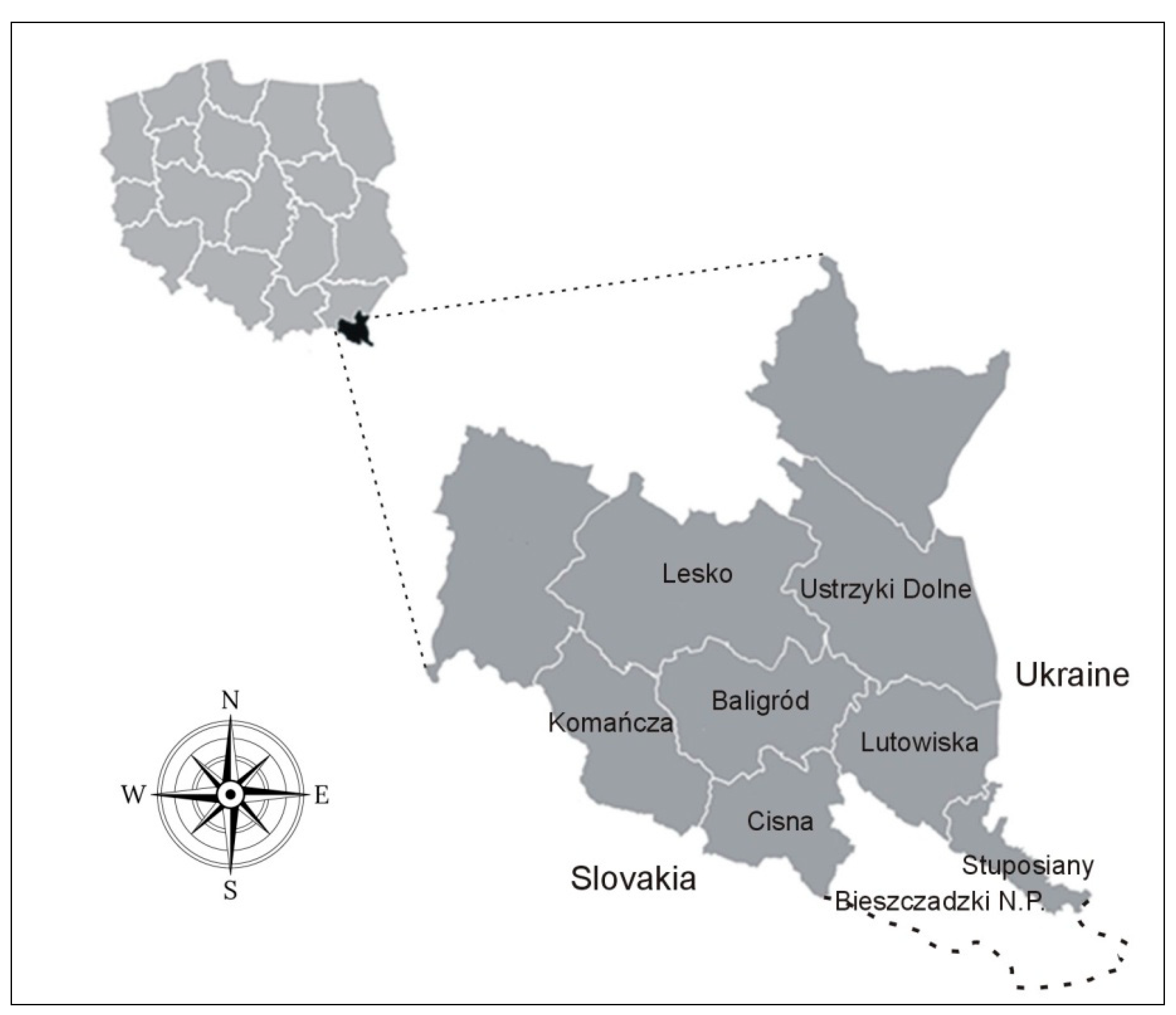
Figure 2.
Spatial distribution of free ranging wisent presence (black triangles – Baligód herd, black dots – Tworylne herd) recorded in the Bieszczady Mountains between 2002 and 2021. Green areas represent forests, white – open land, blue – lakes and watercourses, and red – local settlements, (a) – vegetative season, (b) – winter season.
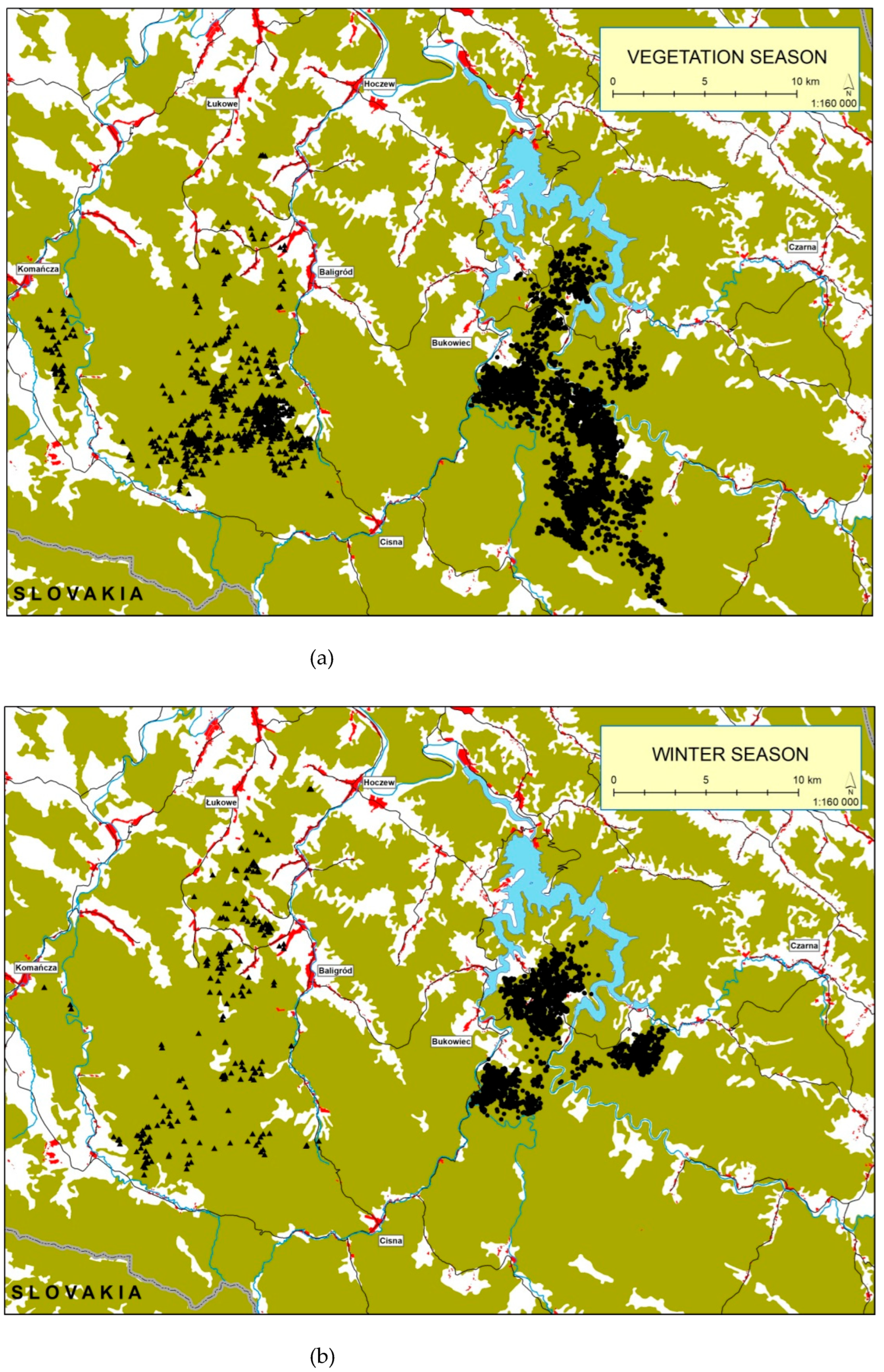
Figure 3.
Confusion matrix for two classes.
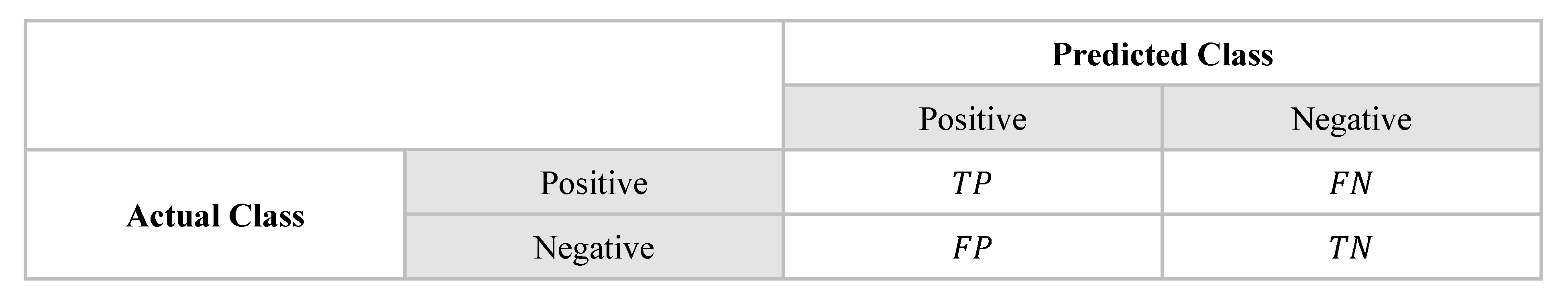
Figure 4.
Learning curves of the XGBoost model obtained for both training and test sets. The x-axis is the number of trees added to the ensemble and the y-axis is the logloss of the model, (a) – vegetative season, (b) – winter season.
Figure 4.
Learning curves of the XGBoost model obtained for both training and test sets. The x-axis is the number of trees added to the ensemble and the y-axis is the logloss of the model, (a) – vegetative season, (b) – winter season.
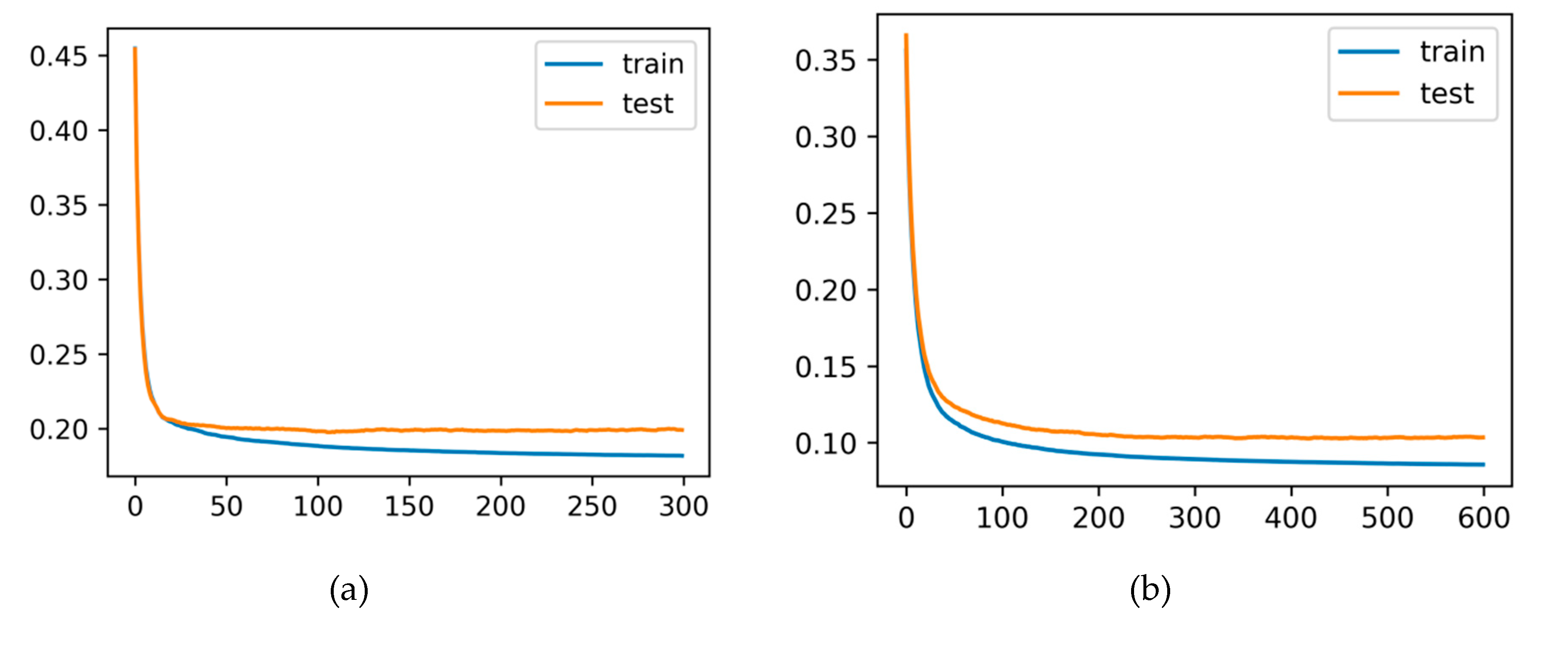

Table 1.
Wisent presence records as assigned to the two subpopulations and to both analysed seasons (numbers) and in total.
Table 1.
Wisent presence records as assigned to the two subpopulations and to both analysed seasons (numbers) and in total.
| Subpopulation | Vegetative season | Winter season | Total |
|---|---|---|---|
| Baligórd herd | 5433 | 1830 | 7263 |
| Tworylne herd | 12304 | 11913 | 24217 |
| Total | 17737 | 13743 | 31480 |
Table 2.
A comparison of elevations above sea level [m], characteristic for the home ranges of the Baligród and Tworylne herds in vegetative (March-October) and winter (November-February) seasons.
Table 2.
A comparison of elevations above sea level [m], characteristic for the home ranges of the Baligród and Tworylne herds in vegetative (March-October) and winter (November-February) seasons.
| Subpopulation | Vegetative season Elevation a.s.l. [m] |
Winter season Elevation a.s.l. [m] |
Total | ||
|---|---|---|---|---|---|
| Mean ± SD | n | Mean ± SD | n | ||
| Baligórd herd | 712.47 ± 90.06 | 5433 | 686.46 ± 98.79 | 1830 | 7263 |
| Tworylne herd | 651.54 ± 160.37 | 12304 | 568.46 ± 58.72 | 11913 | 24217 |
Table 3.
Land cover characteristics of the home ranges of the Baligród and Tworylne herds according to CLC level 1 inventory classification – for the vegetative season.
Table 3.
Land cover characteristics of the home ranges of the Baligród and Tworylne herds according to CLC level 1 inventory classification – for the vegetative season.
| No | CLC 1evel 1 | Baligród herd | Tworylne herd | Total | ||
|---|---|---|---|---|---|---|
| n | % | n | % | |||
| 1 | Artificial surfaces | 0 | 0.00% | 0 | 0.0% | 0 |
| 2 | Agricultural areas | 542 | 9.98% | 1744 | 14.17% | 2286 |
| 3 | Forest and semi natural areas | 4891 | 90.02% | 10484 | 85.21% | 15375 |
| 5 | Water bodies | 0 | 0.00% | 76 | 0.62% | 76 |
| Total | 5433 | 100% | 12304 | 100% | 17737 | |
Table 4.
Land cover characteristics of the home ranges of the Baligród and Tworylne herds according to CLC level 1 inventory classification – for the winter season.
Table 4.
Land cover characteristics of the home ranges of the Baligród and Tworylne herds according to CLC level 1 inventory classification – for the winter season.
| No | CLC level 1 | Baligród herd | Tworylne herd | Total | ||
|---|---|---|---|---|---|---|
| n | % | n | % | |||
| 1 | Artificial surfaces | 0 | 0.00% | 2 | 0.02% | 2 |
| 2 | Agricultural areas | 57 | 3.11% | 325 | 2.73% | 382 |
| 3 | Forest and semi natural areas | 1773 | 96.89% | 11582 | 97.22% | 13355 |
| 5 | Water bodies | 0 | 0.00% | 4 | 0.03% | 4 |
| Total | 1830 | 100% | 11913 | 100% | 13743 | |
Table 5.
Land cover characteristics of the home ranges of the Baligród and Tworylne herds according to CLC level 2 inventory classification – for the vegetative season.
Table 5.
Land cover characteristics of the home ranges of the Baligród and Tworylne herds according to CLC level 2 inventory classification – for the vegetative season.
| No | CLC level 2 | Baligród herd | Tworylne herd | Total | ||
|---|---|---|---|---|---|---|
| n | % | n | % | |||
| 1.1 | Urban fabric | 0 | 0.0% | 0 | 0.0% | 0 |
| 2.1 | Arable land | 1 | 0.02% | 331 | 2.69% | 332 |
| 2.3 | Pastures | 541 | 9.96% | 1403 | 11.40% | 1944 |
| 2.4 | Heterogeneous agricultural areas | 0 | 0.03% | 10 | 0.08% | 10 |
| 3.1 | Forests | 4881 | 89.94% | 10212 | 82.99% | 15093 |
| 3.2 | Scrub and/or herbaceous vegetation association | 10 | 0.18% | 272 | 2.21% | 282 |
| 5.1 | Inland waters | 0 | 0.00% | 76 | 0.62% | 76 |
| Total | 5433 | 100% | 12304 | 100% | 17737 | |
Table 6.
Land cover characteristics of the home ranges of the Baligród and Tworylne herds according to CLC level 2 inventory classification – for the winter season.
Table 6.
Land cover characteristics of the home ranges of the Baligród and Tworylne herds according to CLC level 2 inventory classification – for the winter season.
| No | CLC level 2 | Baligród herd | Tworylne herd | Total | ||
|---|---|---|---|---|---|---|
| n | % | n | % | |||
| 1.1 | Urban fabric | 0 | 0.0% | 2 | 0.02% | 2 |
| 2.1 | Arable land | 29 | 1.58% | 212 | 1.78% | 241 |
| 2.3 | Pastures | 26 | 1.42% | 101 | 0.85% | 127 |
| 2.4 | Heterogeneous agricultural areas | 2 | 0.11% | 12 | 0.10% | 14 |
| 3.1 | Forests | 1767 | 96.56% | 11582 | 97.22% | 13349 |
| 3.2 | Scrub and/or herbaceous vegetation association | 6 | 0.33% | 0 | 0.0% | 6 |
| 5.1 | Inland waters | 0 | 0.0% | 4 | 0.03% | 4 |
| Total | 1830 | 100% | 11913 | 100% | 13743 | |
Table 7.
Land cover characteristics of the home ranges of the Baligród and Tworylne herds according to CLC level 3 inventory classification – for the vegetative season.
Table 7.
Land cover characteristics of the home ranges of the Baligród and Tworylne herds according to CLC level 3 inventory classification – for the vegetative season.
| No | CLC level 3 | Baligród herd | Tworylne herd | Total | ||
|---|---|---|---|---|---|---|
| n | % | n | % | |||
| 1.1.2 | Discontinuous urban fabric | 0 | 0.0% | 0 | 0.0% | 0 |
| 2.1.1 | Non-irrigated arable land | 1 | 0.02% | 331 | 2.69% | 332 |
| 2.3.1 | Pastures | 541 | 9.96% | 1403 | 11.40% | 1944 |
| 2.4.3 | Land principally occupied by agriculture, with significant areas of natural vegetation | 0 | 0.0% | 10 | 0.08% | 10 |
| 3.1.1 | Broad-leaved forest | 1152 | 21.2% | 3176 | 25.81% | 4328 |
| 3.1.2 | Coniferous forest | 2250 | 41.41% | 644 | 5.23% | 2894 |
| 3.1.3 | Mixed forest | 1479 | 27.22% | 6392 | 51.95% | 7871 |
| 3.2.1 | Natural grasslands | 0 | 0.0% | 8 | 2.15% | 8 |
| 3.2.4 | Transitional woodland-shrub | 10 | 0.18% | 264 | 0.62% | 274 |
| 5.1.1 | Water courses | 0 | 0.0% | 76 | 0.62% | 76 |
| 5.1.2 | Water bodies | 0 | 0.0% | 0 | 0% | 0 |
| Total | 5433 | 100% | 12304 | 100% | 17737 | |
Table 8.
Land cover characteristics of the home ranges of the Baligród and Tworylne herds according to CLC level 3 inventory classification – for the winter season.
Table 8.
Land cover characteristics of the home ranges of the Baligród and Tworylne herds according to CLC level 3 inventory classification – for the winter season.
| No | CLC level 3 | Baligród herd | Tworylne herd | Total | ||
|---|---|---|---|---|---|---|
| n | % | n | % | |||
| 1.1.2 | Discontinuous urban fabric | 0 | 0.0% | 2 | 0.01% | 2 |
| 2.1.1 | Non-irrigated arable land | 29 | 1.58% | 212 | 1.77% | 241 |
| 2.3.1 | Pastures | 26 | 1.42% | 101 | 0.85% | 127 |
| 2.4.3 | Land principally occupied by agriculture, with significant areas of natural vegetation | 2 | 0.1% | 12 | 0.10% | 14 |
| 3.1.1 | Broad-leaved forest | 618 | 33.77% | 4430 | 37.19% | 5048 |
| 3.1.2 | Coniferous forest | 538 | 29.39% | 2733 | 22.94% | 3271 |
| 3.1.3 | Mixed forest | 611 | 33.39% | 4419 | 37.09% | 5030 |
| 3.2.1 | Natural grasslands | 6 | 0.33% | 0 | 0.0% | 6 |
| 3.2.4 | Transitional woodland-shrub | 0 | 0.0% | 0 | 0.0% | 0 |
| 5.1.1 | Water courses | 0 | 0.0% | 2 | 0.01% | 2 |
| 5.1.2 | Water bodies | 0 | 0.0% | 2 | 0.01% | 2 |
| Total | 1830 | 100% | 11913 | 100% | 13743 | |
Table 9.
The optimal hyperparameter values of the XGBoost model for the vegetative and winter season.
Table 9.
The optimal hyperparameter values of the XGBoost model for the vegetative and winter season.
| Vegetative season | Winter season |
|---|---|
| subsample = 0.8 n_estimators = 300 min_child_weight = 5 max_depth = 8 learning_rate = 0.3 colsample_bytree = 1 |
subsample = 0.6 n_estimators = 600 min_child_weight = 1 max_depth = 8 learning_rate = 0.1 colsample_bytree = 1 |
Table 10.
Evaluation metrics of the XGBoost model for the vegetative and winter seasons.
| Metric | Vegetative seasons | Winter seasons | ||
|---|---|---|---|---|
| Training set | Test set | Training set | Test set | |
| Accuracy | 91.70% | 91.63% | 96.95% | 96.01% |
| Precision | 88.48% | 88.91% | 92.57% | 90.99% |
| Recall | 83.84% | 82.92% | 83.55% | 79.11% |
| Specificity | 95.17% | 95.46% | 98.98% | 98.73% |
| F1-score | 86.10% | 85.81% | 87.83% | 84.64% |
| ROC-AUC | 90.72% | 89.05% | 91.39% | 89.34% |
Table 11.
Confusion matrix of the XGBoost model for the vegetative season – the test set.
| Predicted Class | |||
|---|---|---|---|
| Baligród herd | Tworylne herd | ||
| Actual Class | Baligród herd | 898 (83%) | 185 (17%) |
| Tworylne herd | 112 (5%) | 2353 (95%) | |
Table 12.
Confusion matrix of the XGBoost model for the winter season – the test set.
| Predicted Class | |||
|---|---|---|---|
| Baligród herd | Tworylne herd | ||
| Actual Class | Baligród herd | 303 (79%) | 80 (21%) |
| Tworylne herd | 30 (1%) | 2336 (99%) | |
Table 13.
Evaluation metrics of the logistic regression for the vegetative and winter seasons.
| Metric | Vegetative seasons | Winter seasons | ||
|---|---|---|---|---|
| Training set | Test set | Training set | Test set | |
| Accuracy | 71.67% | 70.86% | 88.76% | 87.56% |
| Precision | 67.15% | 58.57% | 64.09% | 61.20% |
| Recall | 16.74% | 15.69% | 33.17% | 29.24% |
| Specificity | 96.33% | 95.12% | 97.18% | 97.00% |
| F1-score | 26.80% | 24.75% | 43.72% | 39.58% |
| ROC-AUC | 56.18% | 55.14% | 65.18% | 63.12% |
Disclaimer/Publisher’s Note: The statements, opinions and data contained in all publications are solely those of the individual author(s) and contributor(s) and not of MDPI and/or the editor(s). MDPI and/or the editor(s) disclaim responsibility for any injury to people or property resulting from any ideas, methods, instructions or products referred to in the content. |
© 2025 by the authors. Licensee MDPI, Basel, Switzerland. This article is an open access article distributed under the terms and conditions of the Creative Commons Attribution (CC BY) license (http://creativecommons.org/licenses/by/4.0/).
Copyright: This open access article is published under a Creative Commons CC BY 4.0 license, which permit the free download, distribution, and reuse, provided that the author and preprint are cited in any reuse.


