New Concept of Relativity of Time Applied to Navier-Stokes Equations

1. Introduction

We consider the periodic three-dimensional Navier-Stokes system:

$$\left(NS\right)\left\{\begin{array}{c}{\displaystyle \frac{\partial u}{\partial t}-\nu \Delta u+(u·\nabla )u=-\nabla p,(t,x)\in {\mathbb{R}}_{+}\times {\mathbb{T}}^3}\hfill \\ divu=0,(t,x)\in {\mathbb{R}}_{+}\times {\mathbb{T}}^3\hfill \\ {u|}_{t=0}=u_0\left(x\right),x\in {\mathbb{T}}^3.\hfill \end{array}\right.$$

Here $\nu >0$ represents the fluid viscosity, $u(t,x)$ is a three-dimensional unknown vector-field representing the velocity of the fluid at time t and position $x=(x_1,x_2,x_3)$, $p(t,x)$ is an unknown scalar which stands for the pressure of the fluid at time t and position x, and the system is subject to periodic boundary conditions with basic domain ${\mathbb{T}}^3={[0,2\pi L]}^3$.

We recall that the pressure can be eliminated by projecting $\left(NS\right)$ onto the space of free divergence vector fields, using the Leray projector $\mathbb{P}.$ Thus, it will be convenient dealing with the following equivalent system

$$\begin{array}{cc}\hfill & {\displaystyle \frac{\partial u}{\partial t}-\nu \Delta u+\mathbb{P}(u·\nabla )u=0,(t,x)\in {\mathbb{R}}_{+}\times {\mathbb{T}}^3}\hfill \end{array}$$

(1)

$$\begin{array}{cc}\hfill & divu=0,(t,x)\in {\mathbb{R}}_{+}\times {\mathbb{T}}^3\hfill \end{array}$$

(2)

$$\begin{array}{cc}\hfill & {u|}_{t=0}=u_0\left(x\right),x\in {\mathbb{T}}^3.\hfill \end{array}$$

(3)

For an initial data $u_0\in L^2\left({\mathbb{T}}^3\right)$, it was proven long time ago by Leray and Hopf [6,7] that there exists a global weak solution to $\left(NS\right)$. The local in time existence of unique strong solution also was shown in [7]. Other questions such as regularity and stability can be found in [9] and references therein. Gevrey class regularity of strong solutions to ($NS$) was established due to Foias and Temam in [5]. Further results concerning the solutions of the Navier-Stokes equations in Gevrey-Sobolev spaces can be found in [2,3,4]. In this paper, the author establishes a well-posedness result having initial data in Gevrey-Sobolev space $H_{a,s}^r$, where $0<r<1/2$. Moreover, by defining a new concept of time relativity, he proves that the local in time solution already constructed can be extended into a global in time solution by reaching the maximal time of existence without blowing up. It should be emphasized that the new concept of time relativity plays the key role in prolonging the interval of existence time beyond T which makes of it a global existence criterion. However, the new relativity concept is much more since it has the potential to revolutionize the way we think about time. It is also characterized by its ability to explain phenomena that were previously incompletely explained in quantum physics. The hierarchical relativity, the description of which is given in this paper has the potential to bring together researchers from different disciplines and backgrounds, fostering a rich exchange of ideas and perspectives that can lead to novel approaches and solutions to many open problems in physics and mathematics.

One of the most important aspect of Einstein’s theory of general relativity is that time slows down in the presence of a massive object, such as a black hole. This phenomenon, known as gravitational time dilation, occurs because massive objects distort the fabric of space-time, causing time to run more slowly in their vicinity. By delving into the source, we can gain deeper insights into our purpose. In fact, gravitational time dilation phenomenon as described and known to us is not the root cause, but rather a reflection of a deeper pattern. The observed time dilation effect near massive objects suggests a hierarchical nature of time perception, where time is experienced differently depending not only on the gravitational potential of the observer but also on the ability of smaller objects to move and change direction comparatively with massive ones.

In the vast expanse of the universe, a fascinating time pattern emerges, influencing how objects of varying sizes perceive and experience time. Smaller objects, such as quantum particles, interact with time differently compared to their massive counterparts. This is due to their unique ability to move faster and change directions more rapidly than larger entities.

Unlike the notion of a perfectly circular trajectory that applies only to sizeless objects like quantum particles, larger objects, bound by their physicality and mass, cannot attain such an ideal trajectory. As they move through space, they are influenced by gravitational forces, causing deviations from the notion of perfect circular motion.

This concept can also be seen mirrored in the mechanisms of conscious and unconscious reactions within the human body. Conscious reactions are triggered when the size regime aligns with our typical experiences, where we interact with the macroscopic world. In these situations, our minds and bodies are consciously aware of our actions and surroundings. On the other hand, unconscious reactions come into play when the neural regime activates, involving different size scales, such as at the quantum level or microscopic levels. In these instances, our bodily responses are guided by neural processes beyond our conscious awareness, manifesting the intricate interplay between our physical and cognitive aspects.

In the tapestry of biological systems, an intriguing temporal tapestry unfolds, influencing how organisms of various sizes perceive and navigate the passage of time. At the microscopic level, such as within cellular processes, temporal dynamics take on a distinctly nuanced character in comparison to the temporal experiences of larger multicellular organisms. This discrepancy arises from the fundamental disparities in the rates of biochemical reactions and signaling events.

In the microscopic realm of cells, intricate molecular ballets unfold at astonishing speeds. Enzymatic reactions, molecular translocations, and cellular signaling cascades occur in fractions of a second. This rapid pace is not merely a consequence of scale; it’s a reflection of the dynamic and highly regulated nature of cellular life. Small biological entities, akin to quantum particles in the physical realm, exhibit a propensity to interact with time in a manner that defies the leisurely rhythms of larger organisms.

This biological relativity of time, influenced by the scale and complexity of living systems, prompts a profound inquiry into the adaptive significance of temporal dynamics in the evolution of life. From the rapid beat of microscopic life to the slower cadence of larger organisms, the temporal signatures of biological entities weave a rich narrative of adaptation and survival in the ever-changing theater of existence.

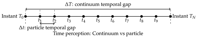
In the realm of fluid mechanics, the concept of time perception at different scales finds profound significance in understanding the behavior of fluid particles and their representation as a continuum. Let’s explore how fluid particles and the representative continuum experience time differently and how the particle’s perspective unveils intermediate instants beyond the continuum’s conscious awareness.

At the microscale level of fluid mechanics, individual fluid particles exhibit dynamic and intricate motions. These particles are subject to Brownian motion, which refers to the random movement of particles driven by collisions with surrounding molecules. At this scale, fluid particles experience time on a highly localized level. They perceive and respond to the forces acting upon them, yielding a detailed and moment-to-moment interaction with their surroundings. On the other hand, at the macroscale, when we consider a continuum representation of fluid, we take into account the average behavior of a vast number of fluid particles. The continuum model simplifies the system, treating the fluid as a continuous medium rather than a collection of discrete particles. In this representation, time is viewed more coarsely, and the continuum evolves smoothly over time, governed by the Navier-Stokes equations or other fluid dynamic models.

Now, let’s delve into how a fluid particle’s perspective contrasts with that of the representative continuum. Imagine a fluid particle as it traverses through the macroscopic fluid continuum. From the particle’s standpoint, time is experienced with a granular focus on instantaneous interactions with neighboring molecules, each encounter influencing its trajectory. As the particle moves through time, it experiences a sequence of intermediate instants that the continuum does not explicitly perceive. These intermediate instants capture the intricacies of individual molecular collisions, local accelerations, and decelerations that contribute to the particle’s trajectory. However, the continuum model glosses over these minute details, treating the fluid’s motion in a more averaged and continuous manner.

Essentially, the continuum experiences time as a macroscopic observer would, recognizing only the fluid’s overall changes at larger scales and time intervals. It misses the rich and complex experiences of fluid particles occurring at much smaller scales. While the continuum’s perspective is valuable for macroscopic analyses and engineering applications, it lacks the fine-grained insights into individual particle behaviors and interactions.

In summary, the study of time perception in fluid mechanics illuminates the contrasting experiences of fluid particles and the representative continuum. At the microscale, fluid particles engage in intricate, localized interactions, perceiving time in a granular manner. In contrast, the continuum representation treats time more coarsely, encapsulating the fluid’s behavior at macroscopic scales. The particle’s perspective offers a deeper understanding of intermediate instants that the continuum does not consciously experience, emphasizing the importance of considering both scales for comprehensive insights into fluid dynamics.

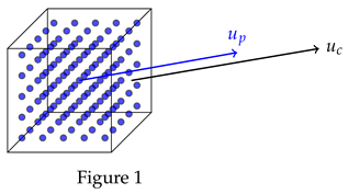Figure 1

Mathematically speaking, two separate locations for the continuum (which is relatively larger in size) should not be conflated with two separate positions of a particle within it (which is much smaller in size). It’s crucial to underscore that, when dealing with a continuum, we shouldn’t perceive a position as a mere point. Let $X_1$ and $X_2$ be two distincts positions of the continuum. Given that the continuum possesses a discernible size, notably larger compared to a particle, it follows that $X_1$ and $X_2$ will occupy a volume in space, implying a non-zero distance, symbolized as l between the centers of these two locations. In contrast, when dealing with particles, their positions can indeed be pinpointed as individual points, and the distance between two distinct particle positions is unequivocally zero. So, we have $\Delta X=X_2-X_1\ge l>0$, while $\Delta x=x_2-x_1\ge 0$. But, since the assemblage of particles, forming the continuum, exists alongside the continuum itself, akin to two adjacent realms. The proximity of these two domains necessitates a symbiotic relationship to maintain the integrity of the entire structure. This phenomenon has been substantiated in a prior works e.g. [9], demonstrating that the Lebesgue measure of a fluid volume, denoted as V remains conserved during the flow process.

Now, consider $u_c$ the velocity of the continuum and $u_p$ the velocity of a particle positioned precisely at the center of the continuum, as illustrated in Figure 1. This particular particle is an integral component of the solid core of the representative elementary continuum, implying that $u_c$ is approximately equal to $u_p$. Having that $u_c\approx {\displaystyle \frac{\Delta X}{\Delta t}}\approx u_p\approx {\displaystyle \frac{\Delta x}{\Delta \tau }}$ and $\Delta X>\Delta x$ yield $\Delta t>\Delta \tau .$ Consequently, the time span between two successive moments for the continuum $\Delta t$ is bigger than the temporal gap between two successive moments for a particle $\Delta \tau$ indicating that the continuum and individual particles possess distinct perceptions of time. This discrepancy in time intervals underscores that each entity operates on a unique time scale. Moreover, this time-scale variation highlights a fascinating phenomenon: particles experience intermediate moments of time that the continuum does not encounter. In essence, particles traverse through a succession of finer temporal increments, capturing subtle interactions and dynamic changes that remain beyond the purview of the continuum’s coarser temporal resolution. This intricate interweaving of time scales deepens our comprehension of fluid dynamics, shedding light on the rich tapestry of behaviors occurring within these systems.

Before we state the main results, we give some notations that we will use throughout the paper. The inhomogeneous Gevrey-Sobolev space is defined, for all $s>1$, $r\in \mathbb{R}$ and the radius of Gevrey class regularity $a\in (0,1)$, by

$$H_{a,s}^r=\{f\in L^2\left({\mathbb{T}}^3\right);e^{a{\Lambda }^{1/s}}f\in H^r\left({\mathbb{T}}^3\right),divf=0\},$$

where $\Lambda$ is the operator $\sqrt{-\Delta }$. The inhomogeneous Gevrey-Sobolev space is equipped with the norm

$${\parallel f\parallel }_{H_{a,s}^r}={\left(\sum _{k\in {\mathbb{Z}}^3}{(1+|k|}^2{)}^r{e}^{{2a|k|}^{1/s}}{|{\widehat{f}}_k|}^2\right)}^{1/2}$$

Naturally, the homogeneous one is given by

$${\dot{H}}_{a,s}^r=\{f\in L^2\left({\mathbb{T}}^3\right);e^{a{\Lambda }^{1/s}}f\in {\dot{H}}^r\left({\mathbb{T}}^3\right),divf=0\}$$

and endowed with the norm

$${\parallel f\parallel }_{{\dot{H}}_{a,s}^r}={\parallel {\Lambda }^r{e}^{a{\Lambda }^{1/s}}f\parallel }_{L^2}={\left(\sum _{k\in {\mathbb{Z}}^3}{|k|}^{2r}{e}^{{2a|k|}^{1/s}}{|{\widehat{f}}_k|}^2\right)}^{1/2},$$

where ${\widehat{f}}_k$ is the $k^{th}$-Fourier coefficient of f, the Lebesgue-Gevrey space $L_{a,s}^2\left({\mathbb{T}}^3\right)$ is the particular case of homogeneous Gevrey-Sobolev space when $r=0$. The Lebesgue-Gevrey space $L_{a,s}^2\left({\mathbb{T}}^3\right)$ is equipped with the inner product

$${\langle f,g\rangle }_{L_{a,s}^2}=\sum _{k\in {\mathbb{Z}}^3}{e}^{{a|k|}^{1/s}}{\widehat{f}}_k\overline{e^{{a|k|}^{1/s}}{\widehat{g}}_k},$$

and the norm

$${\parallel f\parallel }_{L_{a,s}^2}={\left(\sum _{k\in {\mathbb{Z}}^3}{e}^{{2a|k|}^{1/s}}{|{\widehat{f}}_k|}^2\right)}^{1/2}.$$

We need to define the Lei-Lin-Gevrey norm

$${\parallel f\parallel }_{{\chi }_{a,s}^0}=\sum _{k\in {\mathbb{Z}}^3}{e}^{{a|k|}^{1/s}}|{\widehat{f}}_k|.$$

We also recall the Parseval’s relation that will be used in subsequent sections whenever is needed

$${\langle f,g\rangle }_{L^2}={\int }_{{\mathbb{T}}^3}f\left(x\right)\overline{g\left(t\right)}dx=\sum _{k\in {\mathbb{Z}}^3}{\widehat{f}}_k\overline{{\widehat{g}}_k}.$$

Similar notations and definitions can be found in [10,11] and references therein. To ensure the equivalence of homogeneous and non-homogeneous Gevrey-Sobolev norms, we consider initial values with zero spatial means, i.e., we assume that

$${\int }_{{\mathbb{T}}^3}{u}_0\left(x\right)dx=0.$$

Then by using Eq. (1), the spatial periodicity of the solution and the divergence free condition, one obtains

$${\int }_{{\mathbb{T}}^3}u\left(x\right)dx=0.$$

We state here the energy inequality for weak solutions (see e.g. [7,9]),

$$\begin{array}{c}\hfill {\parallel u\left(t\right)\parallel }_{L^2}^2+2\nu {\int }_0^T{\parallel u\left(t\right)\parallel }_{{\dot{H}}^1}^{2}dt\le {\parallel u_0\parallel }_{L^2}^2.\end{array}$$

(4)

The main difficulty encountered to prove our result is that the space we are considering (i.e. $H_{a,s}^r\left({\mathbb{T}}^3\right)$) is not closed under multiplication for $r<1/2$, in fact, the Gevrey-Sobolev space is a Banach algebra only when $r>3/2$ as stated in ([8], Ch. 5, Theorem 5.3). To overcome it, we use the lemma below

Lemma 1. 

For every $\alpha >0$, $s>1,$ and for every k and p in ${\mathbb{Z}}^3$, we have

$$(E_1)\hspace{1em}\hspace{1em}\hspace{1em}\left\{\begin{array}{cc}{e}^{{\alpha |k|}^{{\displaystyle \frac{1}{s}}}}\hfill & \le e^{{\alpha |k-p|}^{{\displaystyle \frac{1}{s}}}}{e}^{{\displaystyle \frac{\alpha }{s}}{|p|}^{{\displaystyle \frac{1}{s}}}},|p|\le |k-p|,\\ e^{{\alpha |k|}^{{\displaystyle \frac{1}{s}}}}\hfill & \le e^{{\displaystyle \frac{\alpha }{s}}{|k-p|}^{{\displaystyle \frac{1}{s}}}}{e}^{{\alpha |p|}^{{\displaystyle \frac{1}{s}}}},|p|\ge |k-p|.\end{array}\right.$$

Proof:

We use the following elementary inequality

$${(1+b)}^{\kappa }\le 1+\kappa b^{\kappa },\forall b,\kappa \in [0,1].$$

Let us start by the case $|p|\le |k-p|$, for which, we have

$$\begin{array}{ccc}{|k|}^{{\displaystyle \frac{1}{s}}}\hfill & =& {|k-p+p|}^{{\displaystyle \frac{1}{s}}}\hfill \\ & \le & {\left(|k-p|+|p|\right)}^{{\displaystyle \frac{1}{s}}}\hfill \\ & \le & {|k-p|}^{{\displaystyle \frac{1}{s}}}{\left(1+{\displaystyle \frac{|p|}{|k-p|}}\right)}^{{\displaystyle \frac{1}{s}}}\hfill \\ \hfill & \le & {|k-p|}^{{\displaystyle \frac{1}{s}}}\left(1+{\displaystyle \frac{1}{s}}{\displaystyle \frac{{|p|}^{\frac{1}{s}}}{{|k-p|}^{\frac{1}{s}}}}\right)\hfill \\ \hfill & =& {|k-p|}^{{\displaystyle \frac{1}{s}}}+{\displaystyle \frac{1}{s}}{|p|}^{{\displaystyle \frac{1}{s}}}.\hfill \end{array}$$

Since $e^{\alpha t}$ is an increasing function with respect to t, it follows that

$$\begin{array}{ccc}{e}^{{\alpha |k|}^{{\displaystyle \frac{1}{s}}}}\hfill & \le & e^{\alpha \left({|k-p|}^{{\displaystyle \frac{1}{s}}}+{\displaystyle \frac{1}{s}}{|p|}^{{\displaystyle \frac{1}{s}}}\right)}\hfill \\ \hfill & =& e^{{\alpha |k-p|}^{{\displaystyle \frac{1}{s}}}}{e}^{{\displaystyle \frac{\alpha }{s}}{|p|}^{{\displaystyle \frac{1}{s}}}}.\hfill \end{array}$$

The second case $|p|\ge |k-p|$ is to be dealt with similarly. □

Lemma 1 turned to be helpful while closing the estimates, and it serves as an effective tool to absorb the exponential weight corresponding to Gevrey norms.

The main result in this paper read

Theorem 1. 

For an arbitrary initial data $u_0\in H_{a,s}^r\left({\mathbb{T}}^3\right)$ such that $div{u}_0=0$, there exists a unique local in time solution to Eq. (1), such that $u\in {\mathcal{C}}^0([0,T);H_{a,s}^r\left({\mathbb{T}}^3\right))\cap L^2(0,T;H_{a,s}^{r+1}\left({\mathbb{T}}^3\right)).$ Moreover, if the initial data $u_0$ satisfies the smallness condition $\parallel u_0{\parallel }_{{\dot{H}}_{a,s}^r}^2<{\displaystyle \frac{\nu }{c}},$ then the existence is global in time.

The proof of theorem 1 is based upon a combination of the Galerkin approximation scheme and a compactness method. A noteworthy challenge we encounter during the analysis is the management of the nonlinear convective term. This term introduces a level of complexity that necessitates careful handling to arrive at the desired result. In order to effectively address this challenge, we make use of Lemma 1. In fact, lemma 1 plays a pivotal role in our approach as it serves as an effective means to absorb the exponential weight that is inherent within the Gevrey space framework.

While Theorem 1 establishes the mathematical well-posedness of the Navier-Stokes equations for local solutions and global under smallness conditions, a deeper understanding of fluid behavior, particularly across scales, is crucial for addressing the challenging problem of extending these local solutions into global ones. In this pursuit, we need the Principle of Hierarchical Relativity of Time (PHRT).

To extend the solution into a global solution, we prove that for each interval of time $[t_k,t_{k+1}]\subset (0,T)$, there exists a threshold m that separates the particle regime and the continuum regime such that if

$$\sum _{|k|\le m}{e}^{a/{s|k|}^{1/s}}|\widehat{u}(k,t)|\le \sum _{|k|>m}{e}^{a/{s|k|}^{1/s}}|\widehat{u}(k,t)|,$$

then the ${\dot{H}}_{a,s}^r$-norm of the solution is non-increasing for all t in $[t_k,t_{k+1}]$. Otherwise, if

$$\sum _{|k|>m}{e}^{a/{s|k|}^{1/s}}|\widehat{u}(k,t)|\le \sum _{|k|\le m}{e}^{a/{s|k|}^{1/s}}|\widehat{u}(k,t)|,$$

then the solution remains controlled $L^2$. But, as when we use Fourier decomposition for u, low-frequency modes ($|k|\le m$) signify large-scale structures. When these large-scale features dominate the solution (meaning high-frequency modes are either cut off or very weak), then the $L^2$-norm and ${\dot{H}}_{a,s}^r$ semi-norm become essentially equivalent. The particularity of the second condition, where the low frequencies part of the solution’s ${\chi }_{a/s,s}^0$-norm outweighs the high frequencies part is that it’s expected to hold true over much longer time intervals than the first condition. This extended validity is precisely why we employ discretization in time for this scenario. Otherwise, if the high frequencies part of the solution’s ${\chi }_{a/s,s}^0$-norm outweighs the low frequencies part, then $t_k$ is allowed to be as close as possible to $t_{k+1}$. Because, this case is regarded as the case where the viscous or the particles regime is the predominant one. Hence, by applying the hierarchical relativity of time explained above and to preserve the space-time ratio ${\displaystyle \frac{\Delta X}{\Delta t}}$ which is the velocity of the representative continuum and the particles within it, the intervals of time on which the first condition holds can be as small as possible while the ones on which the second condition holds cannot. In fact, these interval of time are nothing but the temporal gaps defined earlier associated to a particle when condition 1 holds true or to the representative continuum if condition 2 holds true. Then, the time interval $(0,T)$ is subdivided into alternating temporal gaps in which the ${\dot{H}}_{a,s}^r$-norm of the solution is controlled, depending on whether it corresponds to a particle regime or a larger-scale one.

The remainder of the paper is divided into two sections. The first is assigned to prove local in time existence of the solution. The proof is based on a Galerkin approximation scheme and a standard compactness method to take the limit in the approximating system. The second is devoted to establish a global in time existence criteria based on Fourier analysis.

2. Well Posedness Result

We will use the Galerkin approximation. For $n\in \mathbb{N}$, let $P_n$ be the projection onto the Fourier modes of order up to n, that is

$$P_n\left(\sum _{k\in {\mathbb{Z}}^3}{\widehat{f}}_k{e}^{ix·k}\right)=\sum _{|k|\le n}{\widehat{f}}_k{e}^{ix·k}.$$

Let $u_n=P_{n}u$ be the solution to

$$\begin{array}{c}\hfill {\partial }_t{u}_n+P_n\left[(u_n·\nabla )u_n\right]-\nu \Delta u_n=0\end{array}$$

(5)

$$\begin{array}{c}\hfill u_n\left(0\right)=P_n{u}_0.\end{array}$$

(6)

For some $T_n$, there exists a solution $u_n\in C^{\infty }([0,T_n)\times {\mathbb{T}}^3)$ to this finite-dimensional locally-Lipschitz system of ODEs.

Here and throughout the paper, we will use c to denote a generic positive constant which may depend on a, s and the Sobolev index $r\ge 0$. For the sake of convenience, we use in the following $\mathcal{F}\left(f\right)$ to denote the Fourier transform of f and ${\mathcal{F}}^{-1}\left(f\right)$ its inverse.

2.1. Local in Time Existence

Let us begin by proving the existence of the local in time solution. By taking the $L_{a,s}^2$-inner product of Eq. (5) against $\Lambda u_n$, we get

$$\begin{array}{c}\hfill {\displaystyle \frac{1}{2}}{\displaystyle \frac{d}{dt}}\parallel u_n{\left(t\right)\parallel }_{{\dot{H}}_{a,s}^r}^2+\nu {\parallel u_n\left(t\right)\parallel }_{{\dot{H}}_{a,s}^{r+1}}^2\le \underset{\mathcal{I}}{\underbrace{|{\langle {\Lambda }^r(u_n·\nabla u_n),{\Lambda }^r{u}_n\rangle }_{L_{a,s}^2\left({\mathbb{T}}^3\right)}|}}\end{array}$$

(7)

To estimate the nonlinear term, we proceed as follows

$$\begin{array}{ccc}|{\langle {\Lambda }^r(u_n·\nabla )u_n,{\Lambda }^r{u}_n\rangle }_{L_{a,s}^2}|\hfill & \le & \parallel e^{a{\Lambda }^{1/s}}{\Lambda }^r(u_n·\nabla )u_n{\parallel }_{L^2}{\parallel e^{a{\Lambda }^{1/s}}{\Lambda }^r{u}_n\parallel }_{L^2}.\hfill \end{array}$$

We have

$$\begin{array}{ccc}\parallel e^{a{\Lambda }^{1/s}}{\Lambda }^r(u_n·\nabla )u_n{\parallel }_{L^2}^2\hfill & =& {\displaystyle \sum _{|k|\le n}{e}^{{2a|k|}^{1/s}}{|k|}^{2r}{|\mathcal{F}\left((u·\nabla )u\right)\left(k\right)|}^2}\hfill \\ \hfill & =& {\displaystyle \sum _{|k|\le n}{e}^{{2a|k|}^{1/s}}{|k|}^{2r}{|\mathcal{F}\left(u\right)*\mathcal{F}(\nabla u)\left(k\right)|}^2}\hfill \\ \hfill & \le & {\displaystyle \sum _{|k|\le n}{e}^{{2a|k|}^{1/s}}{|k|}^{2r}{\left(|\mathcal{F}(u)|*|\mathcal{F}(\nabla u)|\right)}^2\left(k\right)}\hfill \\ \hfill & \le & {\displaystyle \sum _{|k|\le n}{e}^{{2a|k|}^{1/s}}{|k|}^{2r}{\left(\sum _p|\widehat{u}(k-p)||p||\widehat{u}\left(p\right)|\right)}^2}\hfill \\ \hfill & \le & {\displaystyle \sum _{|k|\le n}{e}^{{2a|k|}^{1/s}}{|k|}^{2r}(\sum _{|p|\le |k-p|}|\widehat{u}(k-p)||p||\widehat{u}\left(p\right)|}\hfill \\ & & {\displaystyle +\sum _{|p|>|k-p|}|\widehat{u}(k-p)||p||\widehat{u}\left(p\right)|{)}^2}\hfill \end{array}$$

By using lemma 1, we get

$$\begin{array}{ccc}\parallel e^{a{\Lambda }^{1/s}}{\Lambda }^r(u_n·\nabla )u_n{\parallel }_{L^2}^2\hfill & \le & {\displaystyle 16\sum _{|k|\le n}{\left(\sum _{|p|\ge |k-p|}{e}^{\frac{a}{s}{|k-p|}^{1/s}}|\widehat{u}(k-p)|e^{{a|p|}^{1/s}}{|p|}^{r+1}|\widehat{u}\left(p\right)|\right)}^2}\hfill \\ & +& {\displaystyle 16\sum _{|k|\le n}{\left(\sum _{|p|\le |k-p|}{e}^{{a|k-p|}^{1/s}}{|k-p|}^r|\widehat{u}(k-p)|e^{\frac{a}{s}{|p|}^{1/s}}|p||\widehat{u}\left(p\right)|\right)}^2}\hfill \end{array}$$

Using the following notations:

$$\begin{array}{ccc}{\alpha }_1\left(k\right)\hfill & =& e^{{\displaystyle \frac{a}{s}}{|k|}^{1/s}}|\widehat{u}\left(k\right)|\hfill \\ {\alpha }_2\left(k\right)\hfill & =& e^{{a|k|}^{1/s}}{|k|}^{r+1}|\widehat{u}\left(k\right)|\hfill \\ {\alpha }_3\left(k\right)\hfill & =& e^{{a|k|}^{1/s}}{|k|}^r|\widehat{u}\left(k\right)|\hfill \\ {\alpha }_4\left(k\right)\hfill & =& e^{{\displaystyle \frac{a}{s}}{|k|}^{1/s}}|k||\widehat{u}\left(k\right)|,\hfill \end{array}$$

it follows that

$$\begin{array}{ccc}\parallel e^{a{\Lambda }^{1/s}}{\Lambda }^r(u_n·\nabla )u_n{\parallel }_{L^2}^2\hfill & \le & 16\left(\parallel {\alpha }_1*{\alpha }_2{\parallel }_{l^2}^2+{\parallel {\alpha }_3*{\alpha }_4\parallel }_{l^2}^2\right).\hfill \end{array}$$

By applying Young’s convolution inequality, we obtain

$$\begin{array}{ccc}\parallel e^{a{\Lambda }^{1/s}}{\Lambda }^r(u_n·\nabla )u_n{\parallel }_{L^2}^2\hfill & \le & 16\left(\parallel {\alpha }_1{\parallel }_{l^1}^2\parallel {\alpha }_2{\parallel }_{l^2}^2+\parallel {\alpha }_3{\parallel }_{l^2}^2{\parallel {\alpha }_4\parallel }_{l^1}^2\right).\hfill \end{array}$$

We notice that

$$\begin{array}{ccc}\parallel {\alpha }_2{\parallel }_{l^2}\hfill & =& \parallel u_n{\parallel }_{{\dot{H}}_{a,s}^{r+1}},\hfill \end{array}$$

and

$$\begin{array}{ccc}\parallel {\alpha }_3{\parallel }_{l^2}\hfill & =& \parallel u_n{\parallel }_{{\dot{H}}_{a,s}^r}.\hfill \end{array}$$

Let $b=a-{\displaystyle \frac{a}{s}}$, by using Cauchy-Schwarz inequality, we obtain

$$\begin{array}{ccc}\parallel {\alpha }_1{\parallel }_{l^1}\hfill & =& {\displaystyle \sum _{|k|\le n}{e}^{\frac{a}{s}{|k|}^{1/s}}|\widehat{u}\left(k\right)|}\hfill \\ \hfill & =& {\displaystyle \sum _{|k|\le n}{e}^{-{b|k|}^{1/s}}{e}^{{a|k|}^{1/s}}|\widehat{u}\left(k\right)|}\hfill \\ \hfill & \le & \underset{c<\infty }{\underbrace{{\left({\sum }_k{e}^{-{2b|k|}^{1/s}}\right)}^{1/2}}}{\parallel u_n\parallel }_{{\dot{H}}_{a,s}^r},\hfill \end{array}$$

since $0<a<1$ and $s>1$. Thus,

$$\begin{array}{ccc}\parallel {\alpha }_1{\parallel }_{l^1}\hfill & \le & c\parallel u_n{\parallel }_{{\dot{H}}_{a,s}^r}.\hfill \end{array}$$

Similarly, we have

$$\begin{array}{ccc}\parallel {\alpha }_4{\parallel }_{l^1}\hfill & \le & \underset{c<\infty }{\underbrace{{\left(\sum _k{e}^{-{2b|k|}^{1/s}}\right)}^{1/2}}}{\parallel u_n\parallel }_{{\dot{H}}_{a,s}^1}.\hfill \end{array}$$

By using the continuous embedding ${\dot{H}}_{a,s}^{r+1}\left({\mathbb{T}}^3\right)\hookrightarrow {\dot{H}}_{a,s}^1\left({\mathbb{T}}^3\right)$, we obtain

$$\begin{array}{ccc}\parallel {\alpha }_4{\parallel }_{l^1}\hfill & \le & c\parallel u_n{\parallel }_{{\dot{H}}_{a,s}^{r+1}}.\hfill \end{array}$$

Using the above estimates, we get

$$\begin{array}{ccc}\parallel e^{a{\Lambda }^{1/s}}{\Lambda }^r(u_n·\nabla )u_n{\parallel }_{L^2}\hfill & \le & C^{★}\parallel u_n{\parallel }_{{\dot{H}}_{a,s}^r}{\parallel u_n\parallel }_{{\dot{H}}_{a,s}^{r+1}}.\hfill \end{array}$$

By applying Young’s product inequality, we obtain

$$\begin{array}{ccc}{\displaystyle |{\langle {\Lambda }^r(u_n·\nabla )u_n,{\Lambda }^r{u}_n\rangle }_{L_{a,s}^2}|}\hfill & \le & {\displaystyle \frac{C}{2}\parallel u_n{\parallel }_{{\dot{H}}_{a,s}^r}^4+\frac{\nu }{2}{\parallel u_n\parallel }_{{\dot{H}}_{a,s}^{r+1}}^2.}\hfill \end{array}$$

(8)

Here and throughout the paper, we will use c or C to denote a generic positive constant which may depend on a, s, the Sobolev index r and $\nu$. By using (8), we obtain

$$\begin{array}{c}\hfill {\displaystyle \frac{d}{dt}\parallel u_n{\left(t\right)\parallel }_{{\dot{H}}_{a,s}^r}^2+\nu \parallel u_n{\left(t\right)\parallel }_{{\dot{H}}_{a,s}^{r+1}}^2\le C{\parallel u_n\left(t\right)\parallel }_{{\dot{H}}_{a,s}^r}^4.}\end{array}$$

(9)

Now, we compare $\parallel u_n{\parallel }_{{\dot{H}}_{a,s}^r}^2$ with the solution of the problem

$$\begin{array}{c}\hfill {\displaystyle \frac{d\eta }{dt}}=C{\eta }^2,\eta \left(0\right)={\parallel u_0\parallel }_{{\dot{H}}_{a,s}^r}^2,\end{array}$$

and deduce that for all t, such that $0\le Ct\parallel u_0{\parallel }_{{\dot{H}}_{a,s}^r}^2<1$, we have

$$\begin{array}{c}\hfill \parallel u_n{\parallel }_{{\dot{H}}_{a,s}^r}^2\le {\displaystyle \frac{\parallel u_0{\parallel }_{{\dot{H}}_{a,s}^r}^2}{1-Ct\parallel u_0{\parallel }_{{\dot{H}}_{a,s}^r}^2}}.\end{array}$$

In particular, if we choose $T=1/2C\parallel u_0{\parallel }_{{\dot{H}}_{a,s}^r}^2$, then for all $t\in [0,T]$ we have the uniform upper bound

$$\begin{array}{ccc}\hfill \underset{t\in [0,T]}{sup}{\parallel u_n\left(t\right)\parallel }_{{\dot{H}}_{a,s}^r}^2& \le \hfill & \hfill \eta \left(T\right)=2\parallel u_0{\parallel }_{{\dot{H}}_{a,s}^r}^2.\end{array}$$

Now, we integrate (9) over the interval $(0,T)$ to get

$$\begin{array}{c}\hfill {\int }_0^T\parallel u_n{\left(t\right)\parallel }_{{\dot{H}}_{a,s}^{r+1}}^{2}dt\le {\displaystyle \frac{C}{\nu }}{\int }_0^T{\parallel u_n\left(t\right)\parallel }_{{\dot{H}}_{a,s}^r}^{4}dt+{\displaystyle \frac{\parallel u_0{\parallel }_{{\dot{H}}_{a,s}^r}^2}{\nu }}\\ \hfill \le \tilde{\eta }\left(T\right)={\displaystyle \frac{CT{\eta }^2\left(T\right)+\eta \left(T\right)/2}{\nu }}.\end{array}$$

These are uniform bounds on the approximate solution $u_n$ in $L^{\infty }(0,T;{\dot{H}}_{a,s}^r)$ and $L^2(0,T;{\dot{H}}_{a,s}^{r+1})$. In order to use the Aubin-Lions Lemma [1], we find uniform bounds on ${\partial }_t{u}_n$ in $L^2(0,T;H_{a,s}^{-r})$. We will now estimate the norm $\parallel {\partial }_t{u}_n{\parallel }_{{\dot{H}}_{a,s}^{-r}}$ by estimating the viscous term $\Delta u_n$ and the nonlinear term $(u_n·\nabla )u_n$. We have

$$\parallel \Delta u_n{\parallel }_{H_{a,s}^{-r}}\le {\parallel u_n\parallel }_{{\dot{H}}_{a,s}^{r+1}},$$

and

$$\begin{array}{ccc}\hfill \parallel (u_n·\nabla )u_n{\parallel }_{H_{a,s}^{-r}}& \le \hfill & \hfill 2\parallel (u_n·\nabla )u_n{\parallel }_{{\dot{H}}_{a,s}^r}\\ & \le \hfill & \hfill C_{a,s}\parallel u_n{\parallel }_{{\dot{H}}_{a,s}^r}{\parallel u_n\parallel }_{{\dot{H}}_{a,s}^{r+1}}\end{array}$$

As

$${\partial }_t{u}_n=\nu \Delta u_n-P_n\left[(u_n·\nabla )u_n\right],$$

it turns out that

$$\begin{array}{c}\hfill \parallel {\partial }_t{u}_n{\parallel }_{{\dot{H}}_{a,s}^{-r}}\le \nu \parallel u_n{\parallel }_{{\dot{H}}_{a,s}^{r+1}}+C_{a,s}\parallel u_n{\parallel }_{{\dot{H}}_{a,s}^r}{\parallel u_n\parallel }_{{\dot{H}}_{a,s}^{r+1}}.\end{array}$$

Therefore, we obtain

$$\begin{array}{ccc}\hfill {\int }_0^T{\parallel {\partial }_t{u}_n\left(t\right)\parallel }_{{\dot{H}}_{a,s}^{-r}}^{2}dt& \le \hfill & \hfill 2{\nu }^2{\int }_0^T\parallel u_n{\left(t\right)\parallel }_{{\dot{H}}_{a,s}^{r+1}}^{2}dt+2C_{a,s}^2\underset{[0,T]}{sup}\parallel u_n{\left(t\right)\parallel }_{{\dot{H}}_{a,s}^r}^2{\int }_0^T{\parallel u_n\left(t\right)\parallel }_{{\dot{H}}_{a,s}^{r+1}}^{2}dt.\end{array}$$

That is

$$\begin{array}{cc}\hfill & {\int }_0^T{\parallel {\partial }_t{u}_n\left(t\right)\parallel }_{H_{a,s}^{-1}}^{2}dt\le 2\nu \tilde{\eta }\left(T\right)+{\displaystyle \frac{2}{\nu }}{\left(C_{a,s}\right)}^2\eta \left(T\right)\tilde{\eta }\left(T\right).\hfill \end{array}$$

(10)

Then, Aubin-Lions lemma [1] allows to extract a subsequence of $u_n$ that converges strongly to u in $L^2(0,T;H_{a,s}^r)$.

2.2. Continuous Dependence and Uniqueness

To prove continuous dependence on the initial data, we suppose that there exist two different solutions $u_1$ and $u_2$ to Eq. (1) that arose from two different initial data. To be more precise, let us consider two solutions $u_1=u_1(t,x)$ and $u_2=u_2(t,x)$ satisfying Eq. (1) and corresponding to two possibly different initial data $u_1^0=u_1^0\left(x\right)$ and $u_2^0=u_2^0\left(x\right)$. Let $w=u_1-u_2$, subtracting the two equations verified by $u_1$ and $u_2$, and taking the inner product against $\Lambda w$, we obtain

$$\begin{array}{ccc}\langle e^{a{\Lambda }^{1/s}}{\partial }_{t}w,e^{a{\Lambda }^{1/s}}\Lambda w\rangle \hfill & -\nu & {\langle e^{a{\Lambda }^{1/s}}\Delta w,e^{a{\Lambda }^{1/s}}\Lambda w\rangle }_{L^2}+{\langle e^{a{\Lambda }^{1/s}}{\Lambda }^r(u_1·\nabla )w,e^{a{\Lambda }^{1/s}}{\Lambda }^{r}w\rangle }_{L^2}\hfill \\ & +& {\langle e^{a{\Lambda }^{1/s}}{\Lambda }^r(w·\nabla )u_2,e^{a{\Lambda }^{1/s}}{\Lambda }^{r}w\rangle }_{L^2}=0.\hfill \end{array}$$

(11)

The Cauchy-Schwarz inequality yields

$$\begin{array}{ccc}\hfill |{\langle e^{a{\Lambda }^{1/s}}{\Lambda }^r(u_1·\nabla )w,e^{a{\Lambda }^{1/s}}{\Lambda }^{r}w\rangle }_{L^2}|& \le \hfill & \hfill \parallel e^{a{\Lambda }^{1/s}}{\Lambda }^r(u_1·\nabla ){w\parallel }_{L^2}{\parallel e^{a{\Lambda }^{1/s}}{\Lambda }^{r}w\parallel }_{L^2}.\end{array}$$

We use lemma 1 to obtain

$$\parallel e^{a{\Lambda }^{1/s}}{\Lambda }^r(u_1·\nabla ){w\parallel }_{L^2}\le C_{a,s}{\parallel u\parallel }_{{\dot{H}}_{a,s}^r}{\parallel w\parallel }_{{\dot{H}}_{a,s}^{r+1}}.$$

By using Young inequality ($ab\le \epsilon a^2/2+{\displaystyle \frac{1}{\epsilon }}{b}^2/2$), we get

$$\begin{array}{ccc}\hfill |{\langle e^{a{\Lambda }^{1/s}}{\Lambda }^r(u_1·\nabla )w,e^{a{\Lambda }^{1/s}}{\Lambda }^{r}w\rangle }_{L^2}|& \le \hfill & \hfill C_{a,s}^{\nu }\parallel u_1{\parallel }_{{\dot{H}}_{a,s}^r}^2{\parallel w\parallel }_{{\dot{H}}_{a,s}^r}^2+{\displaystyle \frac{\nu }{2}}{\parallel w\parallel }_{{\dot{H}}_{a,s}^{r+1}}^2,\end{array}$$

where $C_{a,s}^{\nu }$ is a positive constant that depends on a, s and $\nu$. The second nonlinear term can be estimated the same manner as we did to estimate the former. Namely, Cauchy-Schwarz inequality yields

$$\begin{array}{ccc}\hfill |{\langle e^{a{\Lambda }^{1/s}}{\Lambda }^r(w·\nabla )u_2,e^{a{\Lambda }^{1/s}}{\Lambda }^{r}w\rangle }_{L^2}|& \le \hfill & \hfill \parallel e^{a{\Lambda }^{1/s}}{\Lambda }^r(w·\nabla )u_2{\parallel }_{L^2}{\parallel e^{a{\Lambda }^{1/s}}{\Lambda }^{r}w\parallel }_{L^2}.\end{array}$$

We use lemma 1 to estimate the quadratic term, we have

$$\parallel e^{a{\Lambda }^{1/s}}{\Lambda }^r(w·\nabla )u_2{\parallel }_{L^2}\le C_{a,s}{\parallel w\parallel }_{{\dot{H}}_{a,s}^r}{\parallel u_2\parallel }_{{\dot{H}}_{a,s}^{r+1}}.$$

Thus,

$$|{\langle e^{a{\Lambda }^{1/s}}{\Lambda }^r(w·\nabla )u_2,e^{a{\Lambda }^{1/s}}{\Lambda }^{r}w\rangle }_{L^2}|\le C_{a,s}\parallel u_2{\parallel }_{{\dot{H}}_{a,s}^{r+1}}{\parallel w\parallel }_{{\dot{H}}_{a,s}^r}^2.$$

By plugging the above estimates into (11), one obtains

$$\begin{array}{c}\hfill {\displaystyle \frac{d}{dt}}{\parallel w\left(t\right)\parallel }_{{\dot{H}}_{a,s}^r}^2+{\nu \parallel w\left(t\right)\parallel }_{{\dot{H}}_{a,s}^{r+1}}^2\le C\left(\parallel u_1{\parallel }_{{\dot{H}}_{a,s}^r}^2+{\parallel u_2\parallel }_{{\dot{H}}_{a,s}^{r+1}}\right)\times {\parallel w\left(t\right)\parallel }_{{\dot{H}}_{a,s}^r}^2.\end{array}$$

In particular, we get by using the Gronwall lemma

$$\begin{array}{c}\hfill {\parallel w\left(t\right)\parallel }_{{\dot{H}}_{a,s}^r}^2\le {\parallel w\left(0\right)\parallel }_{{\dot{H}}_{a,s}^r}^{2}exp\left(C{\int }_0^t\Gamma \left(\tau \right)d\tau \right),\end{array}$$

where

$$\Gamma \left(\tau \right)=\parallel u_1{\left(\tau \right)\parallel }_{{\dot{H}}_{a,s}^r}^2+{\parallel u_2\left(\tau \right)\parallel }_{{\dot{H}}_{a,s}^{r+1}}.$$

Continuous dependence on initial data follows since $u_1$ and $u_2$ are in $L_T^{\infty }\left({\dot{H}}_{a,s}^r\right)\cap L_T^2\left({\dot{H}}_{a,s}^{r+1}\right)$. In particular, we get uniqueness when $u_1^0=u_2^0$.

2.3. Global in Time Existence Result

At this point, we have proved that for initial data $u_0\in H_{a,s}^r\left({\mathbb{T}}^3\right)$, there exists a unique local solution $u\in {\mathcal{C}}^0([0,T),H_{a,s}^r)\cap L^2(0,T;H_{a,s}^{r+1})$ to (1). It remains to prove that u can be extended to a global solution, when the initial data is as small as required. To do so, let us take the ${\dot{H}}_{a,s}^r$-inner product of Eq. 5 against u to obtain

$$\begin{array}{c}\hfill {\displaystyle \frac{1}{2}}{\displaystyle \frac{d}{dt}}{\parallel u\left(t\right)\parallel }_{{\dot{H}}_{a,s}^r}^2+\nu {\parallel u\left(t\right)\parallel }_{{\dot{H}}_{a,s}^{r+1}}^2\le \underset{\mathcal{N}}{\underbrace{|{\langle {\Lambda }^r(u·\nabla )u,{\Lambda }^{r}u\rangle }_{L_{a,s}^2\left({\mathbb{T}}^3\right)}|}}.\end{array}$$

Cauchy-Schwarz inequality yields

$$\begin{array}{ccc}\hfill \mathcal{N}& \le \hfill & \hfill {\parallel (u·\nabla )u\parallel }_{{\dot{H}}_{a,s}^r}{\parallel u\parallel }_{{\dot{H}}_{a,s}^r}.\end{array}$$

By employing lemma 1, we get

$${\parallel (u·\nabla )u\parallel }_{{\dot{H}}_{a,s}^r}\le C_{a,s}{\parallel u\parallel }_{{\dot{H}}_{a,s}^r}{\parallel u\parallel }_{{\dot{H}}_{a,s}^{r+1}}.$$

Since ${\parallel u\parallel }_{{\dot{H}}_{a,s}^r}\le {\parallel u\parallel }_{{\dot{H}}_{a,s}^{r+1}}$, we obtain

$$\mathcal{N}\le C_{a,s}{\parallel u\left(t\right)\parallel }_{{\dot{H}}_{a,s}^r}{\parallel u\left(t\right)\parallel }_{{\dot{H}}_{a,s}^{r+1}}^2.$$

If one starts from an initial data such that $\parallel u_0{\parallel }_{{\dot{H}}_{a,s}^r}<\nu /C_{a,s},$ then the coefficient $\left(\nu -C_{a,s}{\parallel u\left(t\right)\parallel }_{{\dot{H}}_{a,s}^r}\right)$ still positive at least over a short interval of time $[0,\tau ]\subset [0,T)$. In that case, it holds that ${\displaystyle \frac{d}{dt}{\parallel u\left(t\right)\parallel }_{{\dot{H}}_{a,s}^r}^2\le 0.}$ By using a continuity argument, the condition ${\parallel u\left(t\right)\parallel }_{{\dot{H}}_{a,s}^r}<{\displaystyle \frac{\nu }{C_{a,s}}}$ holds true on $[0,T)$ which rules out the blowup of ${\parallel u\left(t\right)\parallel }_{{\dot{H}}_{a,s}^r}^2$ when t approaches T or for any $t\in {\mathbb{R}}_{+}$.

3. Complementary Result (PHRT)

We recall that it holds that

$$\begin{array}{c}\hfill {\displaystyle \frac{1}{2}}{\displaystyle \frac{d}{dt}}{\parallel u\left(t\right)\parallel }_{{\dot{H}}_{a,s}^r}^2+\nu {\parallel u\left(t\right)\parallel }_{{\dot{H}}_{a,s}^{r+1}}^2\le |{\langle {\Lambda }^r(u·\nabla )u,{\Lambda }^{r}u\rangle }_{L_{a,s}^2\left({\mathbb{T}}^3\right)}|\end{array}$$

By using the Cauchy-Scwarz inequality, we have

$$\begin{array}{c}\hfill |{\langle {\Lambda }^r(u·\nabla u),{\Lambda }^{r}u\rangle }_{L_{a,s}^2\left({\mathbb{T}}^3\right)}{|\le \parallel (u·\nabla )u\parallel }_{{\dot{H}}_{a,s}^r}{\parallel u\parallel }_{{\dot{H}}_{a,s}^r}.\end{array}$$

By using lemma 1 to control the exponential factor, we get

$$\begin{array}{ccc}{\parallel (u·\nabla )u\parallel }_{{\dot{H}}_{a,s}^r}^2\hfill & \le & {\displaystyle 16\sum _k{\left(\sum _{|p|\ge |k-p|}{e}^{\frac{a}{s}{|k-p|}^{1/s}}|\widehat{u}(k-p)|e^{{a|p|}^{1/s}}{|p|}^{r+1}|\widehat{u}\left(p\right)|\right)}^2}\hfill \\ & +& {\displaystyle 16\sum _k{\left(\sum _{|p|\le |k-p|}{e}^{{a|k-p|}^{1/s}}{|k-p|}^{r+1}|\widehat{u}(k-p)|e^{\frac{a}{s}{|p|}^{1/s}}|\widehat{u}\left(p\right)|\right)}^2}\hfill \\ \hfill & \le & {\displaystyle 32{\left({\displaystyle \sum _k{e}^{\frac{a}{s}{|k|}^{1/s}}|\widehat{u}\left(k\right)|}\right)}^2\sum _k{e}^{{2a|k|}^{1/s}}{|k|}^{2(r+1)}{|\widehat{u}\left(k\right)|}^2}\hfill \\ \hfill & =& {32\parallel u\left(t\right)\parallel }_{{\chi }_{a,s}^0}^2{\parallel u\parallel }_{{\dot{H}}_{a,s}^{r+1}}^2.\hfill \end{array}$$

For a certain number m (to be discussed later on), we have

$$\begin{array}{ccc}\hfill \sum _k{e}^{{\displaystyle \frac{a}{s}}{|k|}^{1/s}}|\widehat{u}(t,k)|& =\hfill & \hfill \sum _{|k|\le m}{e}^{{\displaystyle \frac{a}{s}}{|k|}^{1/s}}|\widehat{u}(t,k)|+\sum _{|k|>m}{e}^{{\displaystyle \frac{a}{s}}{|k|}^{1/s}}|\widehat{u}(t,k)|.\end{array}$$

Two possible natural cases may occur. The first case is when the major amount of energy at time t is concentrated in high-frequency components. That is,

$$\begin{array}{c}\hfill \sum _{|k|\le m}{e}^{{\displaystyle \frac{a}{s}}{|k|}^{1/s}}|\widehat{u}(t,k)|\le \sum _{|k|>m}{e}^{{\displaystyle \frac{a}{s}}{|k|}^{1/s}}|\widehat{u}(t,k)|.\end{array}$$

(12)

The second is when the major amount of energy at the instant t is clustered in low-frequency components. This case can be represented by the following inequality:

$$\begin{array}{c}\hfill \sum _{|k|>m}{e}^{{\displaystyle \frac{a}{s}}{|k|}^{1/s}}|\widehat{u}(t,k)|\le \sum _{|k|\le m}{e}^{{\displaystyle \frac{a}{s}}{|k|}^{1/s}}|\widehat{u}(t,k)|.\end{array}$$

(13)

Let us suppose that condition (12) holds true on an interval of time $[t_0,t_1]\subset [0,T)$. In that case, we have

$${\parallel u\left(t\right)\parallel }_{{\chi }_{a,s}^0}\le 2\sum _{|k|>m}{e}^{{\displaystyle \frac{a}{s}}{|k|}^{1/s}}|\widehat{u}(t,k)|.$$

Consequently,

$$\begin{array}{c}\hfill {\displaystyle \frac{1}{2}}{\displaystyle \frac{d}{dt}}{\parallel u\left(t\right)\parallel }_{{\dot{H}}_{a,s}^r}^2+{\nu \parallel u\left(t\right)\parallel }_{{\dot{H}}_{a,s}^{r+1}}^2\le 2\sqrt{32}\left(\sum _{|k|>m}{e}^{{\displaystyle \frac{a}{s}}{|k|}^{1/s}}|\widehat{u}(t,k)|\right){\parallel u\left(t\right)\parallel }_{{\dot{H}}_{a,s}^r}{\parallel u\left(t\right)\parallel }_{{\dot{H}}_{a,s}^{r+1}}.\end{array}$$

By using the fact that ${\parallel u\parallel }_{{\dot{H}}_{a,s}^r}\le {\parallel u\parallel }_{{\dot{H}}_{a,s}^{r+1}}$, we get

$$\begin{array}{c}\hfill {\displaystyle \frac{1}{2}}{\displaystyle \frac{d}{dt}}{\parallel u\left(t\right)\parallel }_{{\dot{H}}_{a,s}^r}^2+\left(\nu -2\sqrt{32}\sum _{|k|>m}{e}^{{\displaystyle \frac{a}{s}}{|k|}^{1/s}}|\widehat{u}(t,k)|\right){\parallel u\left(t\right)\parallel }_{{\dot{H}}_{a,s}^{r+1}}^2\le 0.\end{array}$$

By applying the Cauchy-Schwarz inequality, we have

$$\begin{array}{ccc}\hfill \sum _{|k|>m}{e}^{{\displaystyle \frac{a}{s}}{|k|}^{1/s}}|\widehat{u}(t,k)|& \le \hfill & \hfill {\left(\sum _{|k|>m}{\displaystyle \frac{e^{-{2b|k|}^{1/s}}}{{|k|}^{2r}}}\right)}^{1/2}\times {\left(\sum _{|k|>m}{e}^{{2a|k|}^{1/s}}{|k|}^{2r}{|{\widehat{u}}_k|}^2\right)}^{1/2}={\lambda }_m{\parallel u\left(t\right)\parallel }_{{\dot{H}}_{a,s}^r},\end{array}$$

where $b=a-{\displaystyle \frac{a}{s}}$ and ${\lambda }_m=\sqrt{{\sum }_{|k|>m}{\displaystyle \frac{e^{-{2b|k|}^{1/s}}}{{|k|}^{2r}}}}$. Since $\underset{m\to \infty }{lim}{\lambda }_m=0$, then for m such that

$$\nu >2\sqrt{32}{\lambda }_m{\parallel u\left(t_0\right)\parallel }_{{\dot{H}}_{a,s}^r},$$

the factor $\left(\nu -2\sqrt{32}{\lambda }_m{\parallel u\left(t\right)\parallel }_{{\dot{H}}_{a,s}^r}\right)$ still positive at least over a short interval of time $[t_0,{\tau }_1]\subset [t_0,t_1]$. Consequently, it turns out that

$${\displaystyle \frac{d}{dt}}{\parallel u\left(t\right)\parallel }_{{\dot{H}}_{a,s}^r}^2\le 0,forallt\in [t_0,{\tau }_1].$$

But as ${\parallel u\left(t\right)\parallel }_{{\dot{H}}_{a,s}^r}^2$ is continuous on $[t_0,t_1]$, we obtain

$${\parallel u\left(t\right)\parallel }_{{\dot{H}}_{a,s}^r}^2\le {\parallel u\left(t_0\right)\parallel }_{{\dot{H}}_{a,s}^r}^{2}forallt\in [t_0,t_1].$$

Thus, the condition on m has been determined successfully. In fact, the threshold m that separates the two regimes must satisfy

$$\nu >2\sqrt{32}{\lambda }_m{\parallel u\left(t_0\right)\parallel }_{{\dot{H}}_{a,s}^r},$$

which is possible since ${\lambda }_m^2$ is a convergent series (e.g. ${\displaystyle m=\underset{m^{*}}{min}\left\{m^{*};\nu \ge 12{\lambda }_{m^{*}}{\parallel u\left(t_0\right)\parallel }_{{\dot{H}}_{a,s}^r}\right\}}$).

Now, let us suppose that condition 13 holds on some interval of time $[t_0,t_1]\subset [0,T)$. Then, the ${\chi }_{a/s,s}^0$ as well as $L^{\infty }$ norms are equivalent in this case. In fact, since we are dealing with a finite dimensional case, then all norms are equivalent. In particular ${\parallel ·\parallel }_{{\chi }_{a/s,s}^0}\equiv {\parallel ·\parallel }_{L^{\infty }}$. So, by applying the hierarchical relativity explained in the introduction, we get

$$u\approx {\displaystyle \frac{\Delta X}{\Delta t}}\approx \parallel u_c{\parallel }_{{\chi }_{a/s,s}^0}\approx {\parallel u_p\parallel }_{{\chi }_{a/s,s}^0}\approx \underset{\Delta \tau \to 0}{lim}{\displaystyle \frac{\Delta x}{\Delta \tau }}$$

Having that $\Delta x$ can be arbitrarily small $\sim 0$ while $\Delta X$ cannot means that there exists $l>0$ such that $\Delta X\ge l$ which requires restructuring the spacetime by also setting $\Delta t\ge h>0$. Hence, the estimate can be obtained by discretization in time. Here, the intervals $[\ell h,(\ell +1\left)h\right]\subset [0,T)$ on which condition (15), where $h>0$ is a constant temporal void associated to the continuum level below which all particles activity is essentially suppressed. We define ${\mathit{u}}^{\ell }$ a representative of the solution u on the interval $[\ell h,(\ell +1\left)h\right]$.

$${\displaystyle \frac{u^{\ell }-u^{\ell -1}}{h}}-\nu \Delta u^{\ell }+\mathcal{B}(u^{\ell },u^{\ell })=0;$$

It can be shown as in [12] that

$$\begin{array}{cc}\hfill {∥u^{\ell }∥}_{L^2\left({\mathbb{T}}^3\right)}^2& +{∥u^{\ell }-u^{\ell -1}∥}_{L^2\left({\mathbb{T}}^3\right)}^2+2h\nu {∥u^{\ell }∥}_{{\dot{H}}^1\left({\mathbb{T}}^3\right)}^2\le {∥u^{\ell -1}∥}_{L^2\left({\mathbb{T}}^3\right)}^2.\hfill \end{array}$$

Moreover, in the Fourier decomposition of u, low-frequency modes ($|k|\le m$) correspond to large-scale structures. When the solution is dominated by low frequencies meaning high-frequency modes are either truncated or sufficiently weak norms $L^2$ and ${\dot{H}}_{a,s}^r$ become effectively equivalent. The ${\dot{H}}_{a,s}^r$ semi-norm, which weights high frequencies more aggressively, behaves similarly to $L^2$ in this regime because the energy is concentrated at large scales, minimizing the impact of high-frequency contributions. Consequently, the ${\dot{H}}_{a,s}^r$-norm of u would reach the maximal time of existence within a finite number of iterations even if the continuum regime persists for almost all t in $[0,T)$ and the solution does not blow-up at any time near T. Otherwise, if the particle regime prevails during certain time intervals on $[0,T)$, it’s actually advantageous. This is because, during these intervals, the ${\dot{H}}_{a,s}^r$-norm of u decreases in that case as proved earlier.

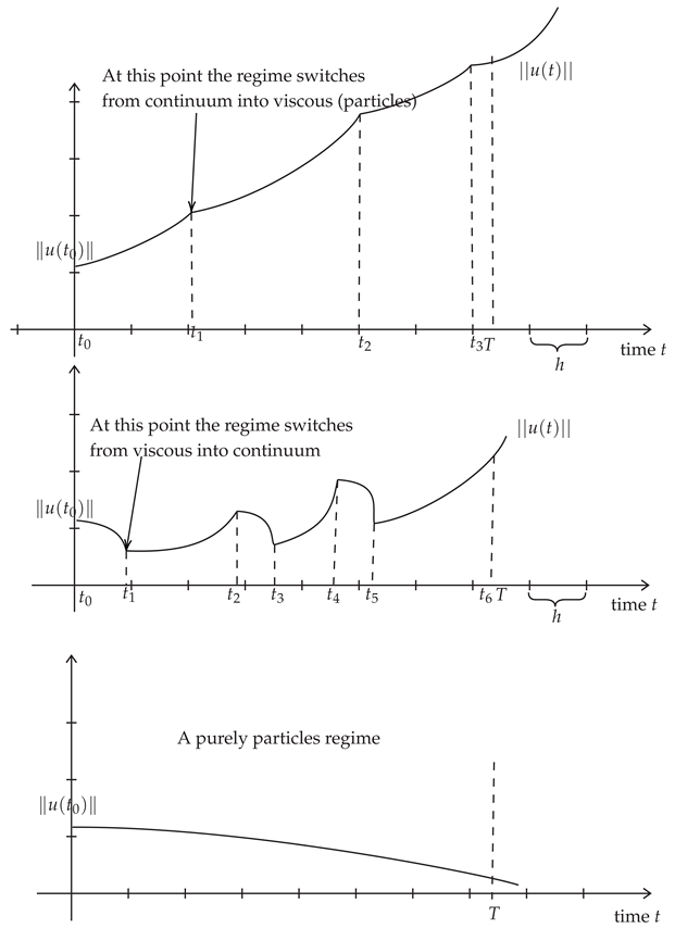
The first curve illustrates the continuum regime where the low frequencies part in ${\displaystyle {\chi }_{a/s}^0}$-norm outweighs the high frequencies part almost for each ${\displaystyle t\in [t_0,T)}$ except for ${\displaystyle t_1}$, ${\displaystyle t_2}$ and ${\displaystyle t_3}$, where the particles regime occurs but it does not last. The second curve illustrates a mixed regime: on ${\displaystyle [t_0,t_1)}$ a particles regime holds, on ${\displaystyle |t_1,t_2)}$ a continuum regime holds, so on and so forth until reaching the maximal time of existence ${\displaystyle T}$. The constant ${\displaystyle h}$ is the temporal gap associated to the continuum, a reason for which each increasing portion of the curve which represents the upper bound on ${||u\left(t\right)||}_{{\dot{H}}_{a,s}^r}$ when the continuum regime holds true should last on an interval of time the length of which is at least ${\displaystyle h}$. The third curve illustrates the case of a purely viscous or particles regime where the high frequencies part in ${\displaystyle {\chi }_{a/s}^0}$-norm outweighs the low frequencies part for all ${\displaystyle t\in [t_0,T)}$, hence ${\displaystyle {||u\left(t\right)||}_{{\dot{H}}_{a,s}^r}}$ is non-increasing as proved.

References

- Aubin, J., 1963. Théorème de compacité. C. R. Acad. Sci. Paris 256, 5042–5044.
- Benameur, J., 2016. On the exponential type explosion of navier-stokes equations. Nonlinear Anal. 103, 87–97.
- Benameur, J., Jlali, L., 2016a. Long time decay for 3d navier-stokes equations in gevrey-sobolev spaces. Electr. j. differ. equ. 104, 1–13.
- Benameur, J., Jlali, L., 2016b. On the blow up criterion of 3d-nse in gevrey-sobolev spaces. J. Math. Fluid Mech. 18, 805–822.
- Foias, C., Temam, R., 1989. Gevrey class regularity for the solutions of the navier-stokes equations. J. Funct. Anal. 87, 359–369.
- Hopf, E., 1951. Über die aufgangswertaufgave für die hydrodynamischen grundliechungen. Math. Nachr. 4, 213–231.
- Leray, J., 1934. Essai sur le mouvement d’un liquide visqueux emplissant l’espace. Acta Math. 63, 193–248.
- Oliver, M., 1996. A Mathematical Investigation of Models of Shallow Water with a Varying Bottom. Ph.d. dissertation, University of Arizona, Tucson, Arizona.
- Robinson, J., Rodrigo, J., Sadowski, W., 2016. The Three-Dimensional Navier-Stokes Equations: Classical Theory. Cambridge University Press, Cambridge.
- Selmi, R., Chaabani, A., 2019. Well-posedness to 3d burgers’ equation in critical gevrey sobolev spaces. Arch. Math.
- Selmi, R., Chaabani, A., 2020. Well-posedness, stability and determining modes to 3d burgers equation in gevrey class. Z. Angew. Math. Phys. 71.
- Temam, R. The Evolution Navier–Stokes Equation, Studies in Mathematics and Its Applications, 2, 1977. [CrossRef]
Disclaimer/Publisher’s Note: The statements, opinions and data contained in all publications are solely those of the individual author(s) and contributor(s) and not of MDPI and/or the editor(s). MDPI and/or the editor(s) disclaim responsibility for any injury to people or property resulting from any ideas, methods, instructions or products referred to in the content. |
© 2025 by the author. Licensee MDPI, Basel, Switzerland. This article is an open access article distributed under the terms and conditions of the Creative Commons Attribution (CC BY) license (https://creativecommons.org/licenses/by/4.0/).
Copyright: This open access article is published under a Creative Commons CC BY 4.0 license, which permit the free download, distribution, and reuse, provided that the author and preprint are cited in any reuse.