Submitted:
01 July 2025
Posted:
02 July 2025
You are already at the latest version
Abstract
The article presents a new approach to the problem of transforming one quantum state into another. It is shown that a r-qubit superposition |x can be obtained from another r-qubit superposition |y, by using only (2r-1) rotations, each presented by one controlled rotation gate. The quantum superpositions with real amplitudes are considered. The traditional two-stage approach Uy-1Ux:|x→|0⊕r→|y requires twice as many rotations. Here, both transformations to the conventual basis state, Ux: |x→ |0⊕r and Uy: |y→ |0⊕r, use (2r-1) rotations each on two binary planes and many of these rotations require additional sets of CNOTs to be represented as 1- or 2-qubit controlled gates. The proposed method is based on the concept of the discrete signal-induced heap transform (DsiHT) which is unitary and generated by a vector and a set of angular equations with given parameters. The quantum analogue of this transform is described. The main characteristic of the DsiHT is the path of processing the data. It is shown that exist such fast paths that allow for effective computing of the DsiHT, which leads to the simple quantum circuits for state preparation and transformation. Examples of such paths are given and quantum circuits for preparation and transformation of 2-, 3-, and 4-qubits are described in detail. CNOT gates are not used, but only controlled gates of elementary rotations around the y-axis. It is shown that the transformation and, in particular, only rotation gates with control qubits are required for initialization of 4-qubits. The quantum circuits are simple and have a recursive form, which makes them easy to implement for arbitrary r-qubit superposition, with r≥2. This approach significantly reduces the complexity of quantum state transformations, paving the way for more efficient quantum algorithms and practical implementations on near-term quantum devices.
Keywords:
qubit state preparation
; quantum state transformation
; quantum signal-induced heap transform
1. Introduction
Quantum state transformation - changing a quantum state through quantum operations or gates - is fundamental to many quantum algorithms. It enables the manipulation and evolution of quantum information, facilitating complex computations. Mastery of state transformations is crucial for multi-qubit systems, which utilize specific gates to create entangled states and perform calculations. It is also vital for quantum error correction to ensure the coherence and fidelity of quantum information. Effective and low-noise state preparation procedures are essential for scalable distribution loading, which underpins a wide range of algorithms that provide a quantum advantage. Therefore, the important step in quantum computation in many applications is the multi-qubit superposition transformation. This is the problem of transformation of one quantum state into another one. Many papers have been published related to this problem [1,2,3,4,5,6,7,8]. Analyzing these works, it is important to note the following. The view has been formed that operations on three or more qubits are very complex for quantum computers. Therefore, when creating quantum circuits, much attention is paid to one- and two-qubit operations, or gates. As a result, each multi-qubit gate, as a unitary transformation, is represented by a chain of single-qubit and dual-qubit gates together with a chain of CNOTs, which may include the long-range CNOTs. The schemes of many simple (for a classical computer) operations have become very complex and are full of such switches of operations from one qubit to another. Therefore, much attention is paid to reducing the number of such gates in quantum circuits [9,10,11]. As is known, the number of elementary rotation gates is around the number and CNOTs in number [12,13,14].
The solution to the problem of multi-qubit state-to-state transformation traditionally lies in the idea of preparing the desired state from the conventional basis state, . Here, is the dimension of the superposition, or the number of qubits it contains. We note the simple method with Givens rotations, . They rotate points inside the unit circle into the interval on the -axis. In matrix theory, such rotations are used in each step of the QR decomposition of a square matrix, when transforming first columns of the submutrix into the vector of form of . We consider only real vectors with norm 1, as for quantum superpositions with real amplitudes. Since it is possible to perform transformations of two vectors and into the unit vector of same dimension,
the transformation , can be fulfilled by the unitary transform . Both transforms and are unitary, and is the inverse of . Moreover, each of them requires rotations with almost the same number of CNOTs, when implementing calculations with 1- and 2-qubit gates [8]. If CNOTs operate not on the adjacent, or nearest-neighbor, bit planes (BP), they can be implemented by a cascade of CNOTs operating on the nearest neighbor bit planes. The permutations with Gray code can be used for this purpose [14,15]. The number of all CNOTs is estimated as [7].
In this work, we analyze the method of rotations and describe the best and fastest, in our opinion, way of elementary rotations for transforming the state. The quantum states, or superpositions of qubits, are considered with real amplitudes. The state-to-state transformation can be performed in one step, which is equivalent to implementing only one transformation which is similar to , instead of two transforms and in the Eq. 1. This is the main goal of this work, not counting and reducing the number of CNOT gates; a lot of work has already been done in this direction. We introduce and describe the new concept of the quantum signal-induced heap transform (QsiHT) which is the analogue of the discrete signal-induced heap transform (DsiHT) [16,17]. With this transform, we show
- How to implement -qubit state-to-state transformation with real amplitudes, by using only elementary rotations, each with only one angle. This number is half as much as the best-known estimation of rotations.
- Visual numerical examples of preparing states for two, three, and four qubits.
- How to initiate any multi-qubit superposition of qubits (without operation of tensor product).
- The importance of the path in -qubit QsiHT and existence of the fast paths for effective computing the QsiHT. For large multi-qubit superpositions, there are various fast paths (with their number increasing with the number of qubits), and we are confident that among them it is possible to choose the most convenient path for implementing state transformations in the topology (architecture) of quantum systems.
- How to build the simple quantum circuits for the -qubit QsiHT.
2. One- and Two-Qubit Operation
In this section, we briefly describe the concept of local gates on single qubits in the quantum superposition [18,19]. The 1- and 2-qubit operators are described by 22 and 44 unitary real or complex matrices, respectively. Let us find out what it means to apply a gate to one qubit in a 4-qubit superposition. Consider the conventional basis of states. In the general case, a 2-qubit superposition may be the Kronecker product of two 1-qubits and , or maybe not. In the first case, the 2-qubit in non-entangled, and in the second case the 2-qubit is entangled. Let , , and denote some unitary operations, that is, 22, 22, and 44 matrices, respectively. If the operation on the non-entangled 2-qubit, that is, 2-qubit superposition, is described by
then, it is the qubit-wise operation, or the operation on two qubits and of . This operation includes the operations on single qubits, too,
As an example, consider the unitary matrix with the real coefficients and The first operation is described in the matrix form as
The circuit element of this gate is shown in Figure 1 in part (a). It is the local gate on the first qubit. Here, is the 22 identity matrix. In the diagram this gate (operator) is connected to the first abstract quantum wire (quantum bit). The circuit element shown in part (b) as the operation on the second qubit. This operation can be written as Note that in general the input, or the 2-qubit superposition , of the circuit does not necessarily have to be entangled. Any 2-qubit superposition is assumed as an input.
The 1-qubit gate controlled by one qubit (or bit) are described by the operation of the Kronecker sum of matrices. The circuit elements in Figure 1(c) and (d) are described in the matrix form as follows:
Note that if a 2-qubit superposition is nonentangled, then may be entangled. These operations are performed on the first or last two amplitudes of , but not on the qubit or . The matrices of the local gates and are more complex than the matrices of the controlled gates and . For instance,
3. Definition of the DsiHT
In this section, we describe the concept of the DsiHT with Givens rotations. We note the following feature of many unitary transformations used in engineering and science. The quantum Fourier transform (QFT) is well-known in quantum computation [20,21,22]. This transform is used in the solution of such problems, as the Shor’s algorithm for integer factorization, the quantum phase estimation algorithm, systems of linear equations and others [23,24,25,26]. The QFT is the quantum analogue of the -point discrete Fourier transform, where integer . The basis functions of the transform are complex exponential functions on the unit circle. Many other discrete unitary transformations also use sets of defined in advance basis functions. We mention for example, the cosine, Hadamard, hartley, cosine and slant transforms [27,28,29]. The -point discrete signal-induced heap transform (DsiHT) generates the basis by a given signal of length . This signal is called the generator of the transform [30,31]. The DsiHT with its simple and fast algorithm (for any order of transformation) is successfully used in many applications in grayscale and color image processing. In addition, the DsiHT can be used for QR-decomposition of square matrices [32]. Together with the generator, the transform uses a parameter which defines the order of processing the input signals. This parameter, or path, is very important and allows us to obtain different QR-decompositions, with diagonal matrices for unitary matrices.
The key of the DsiHT is the generator together with the path. The number of generators can be more than one, but in this work, we focus on the transforms using one pre-selected generator. The selection of the generator depends on the application. For example, in image enhancement, the generators can be defined by the mean or median values along the rows or columns of an image result in very good quality images. The generator-signal is denoted by . The length of the signal is considered to be a power of 2, The basic building blocks that make up the transform are 22 transforms, which can be linear or nonlinear [30]. In this work, we consider 22 rotation matrices, or Givens rotations. The transform is calculated by using Givens rotations by angles . In this case, the signal-generator is presented in its angular representation
plus, the norm, . The signal is considered real. The DsiHT is a unitary transform, , and when applying to the generator, it results in the vector . For a generator with the unit norm or after normalization, this -dimensional vector presents the computational basis state Thus, the following takes place: .
To define the DsiHT, rotations are performed on the generator and at each stage of the transformation one of the two rotation outputs can be reset to zero. For instance, the generator data can be processed in order (it is the path) and , then the updated with , the next updated with , and so on. The illustration of the calculation with the 8-point generator is given in Figure 2. Here, and 22 transforms are rotations by angles . The DsiHT with this regular path is called the DsiHT with weak wheel-carriage [16,31]. The last value is the updated 7 times value of with the splash of energy of the generator, as if we were collecting energy, in one heap.
The DsiHT can be considered as a two-level unitary transformation. First, the angles are calculated from the generator. Then, at each stage of calculation, the transform is applied to the input signal in the way (path) as for the generator. For the DsiHT with the week carriage-wheel, this two-level transform is illustrated in Figure 3, for the case. The results of calculations are
4. The DsiHT with Strong 2-Wheel Carriage
We will consider the concept of the strong DsiHT, or the DsiHT with strong 2-wheel carriage (for more detail, see [16,17]). The path of this DsiHT differs from the path used in the above DsiHT with the week wheel-carriage. As an example, the block-diagram of the 8-point strong DsiHT on its generator is shown in Figure 4. The case of real signals is considered. In this example, on the first step, the angle of the rotation is calculated from the conditions
This transform is the Givens rotation calculated by
with the angle . If the angle or Thus, the angle of rotation is defined from the angular equation Then, the first output, , of the transform is calculated in Eq. 6. On the next step, the second angle of rotation, is calculated from the conditions
Thus, Continuing similar calculations, the last angle of rotation is calculated and then the last value
The value contains information of the energy of the generator.
The input 8-point signal is processed by the same seven rotations in the same order (path). This 2-level strong carriage-wheal DsiHT with processing the input signal with the generator is shown in Figure 5.
In the general case, the -point DsiHT uses basic transformations , regardless of the path of the transform. The transform of the signal-generator equals
where is equal to plus/minus energy of the signal. We consider ; if it is negative, the last angle in rotation can be changed as Thus, the transformation, as well as the signal-generator, are uniquely determined by the data of and the angles of rotations. In other words, the transformation is decoded into the vector For the signal-generator with norm 1, the angular representation holds,
The output is the transform of the input
Note that the above algorithm can be split by two parts. In the first part, all angles of rotation can be calculated from the signal-generator. This is about the angular representation of the generator, . In the second part, the DsiHT of the input signal is calculated,
We now describe the DsiHT in the matrix form. For we denote by the block-diagonal matrix with all 1 in the diagonal and the matrix of rotation in the cell , that is,
The matrix describes the rotation on neighbor bit planes and . For instance, in the case, consider the rotations
The bit planes 0 and 1, or 00 and 01, are adjacent planes, that is, the plane numbers differ by only one bit. The bit planes 1 and 2, or 01 and 10, are not adjacent planes.
In the matrix form, the DsiHT, , is written as the multiplication of block-diagonal matrices with rotations on adjacent planes,
In the case, the 4-point strong DsiHTs with three rotations is written as
Now, we consider an example with the 4-point DsiHT generated by a signal .
Example 1:
Let be the vector-signal with energy and let the input signal be with energy . The DsiHT with the generator has the following matrix:
Here, the diagonal matrix 0.3162,0.1054,0.2981,0.4472. The angles for this transformation are . One can note that the normalized vector-generator lies in the first row of this matrix. The transformation is described by the following decomposition by three rotations:
Consider the permutations and with the matrices
respectively. These two permutations describe the cyclic shifts of a 4-point vector. The following holds for the rotation on the first- and second-bit planes: , that is,
Therefore, the matrix of the 4-point DsiHT is described by three controlled gates as
The transform of the generators is , and for the input signal, . The normalized vectors, and can be considered as 2-qubit superpositions
The 2-qubit QsiHT of these superpositions are and
The quantum scheme of the 2-qubit quantum QsiHT, is given in Figure 6. The flowchart sorts denote the permutations.
IBM’s Qiskit framework is an open-source library in Python for quantum computing developed by IBM [33,34]. It provides tools for building quantum circuits, simulating their behavior, and running them on actual quantum hardware through IBM’s backend. IBM’s Qiskit framework was used to construct and simulate the 2-qubit QsiHT quantum circuit designed to prepare the normalized quantum state corresponding to the vector . The circuit was built using the decomposition of rotation angles through the QsiHT to encode the target amplitudes and its inverse was applied to map the target state onto a computational basis. The simulation involved extracting both the ideal state vector amplitudes and the corresponding measurement probabilities. These were compared against shot-based measurements from simulated runs to assess the accuracy of the circuit. The mean-square root errors (MSRE) between the expected and observed results were computed to quantify the performance of the state preparation. The results of simulation of this circuit in Qiskit are shown in Table 1.
5. Qubits Initiation by the DsiHT
In this section, we consider the inverse DsiHT and describe a simple quantum scheme for initiation of a multi-qubit superposition. Then in Section 6 we show how important it is to choose such a path to make this scheme more efficient.
Let be the -D unit vector which represents the -qubit superposition
Here, the components of the vector are real and complex, and is the conventional basis of states. We consider the case when is real. For the DsiHT generated by this vector, we have
In Example 1, such DsiHT is described for the case, or the 2-qubit superposition . This unitary transformation is real. Therefore, its inverse transformation is defined by the matrix being transpose to , that is, We obtain . Using the property of the inverse operation (transposition), the matrix can be composed by the matrices of rotation by angles as follows:
To initiate the 2-qubit superposition from the first basis state , the quantum circuit of the inverse 2-qubit DsiHT shown in Figure 7 can be used. The angular representation of the signal (or the superposition ) thus allows this superposition to be initiated by three rotations.
In the general case of , the unitary matrix of the DsiHT generated by the real signal is real. Therefore, the inverse DsiHT is described by the matrix transpose to the matrix of the DsiHT and
Example 2:
Consider the 8-D unit vector and the corresponding 3-qubit superposition
For the 8-point strong DsiHT with this generator, the transform matrix can be written as
Seven rotations by the following angles (in degrees) are used:
The transform in the matrix form can be written as
Here, the diagonal matrix
The matrix of the inverse 8-point DsiHT is calculated by seven rotations in reverse order, as
The inverse transform of the first basis state can be written with the diagonal matrix as
This diagonal matrix was introduced to better illustrate the process of constructing this matrix . The first basis function of this transformation is the generator itself (the first column of the matrix). Each next basis function is result of motion of the previous basis functions (for mode detail, see [31]).
Any -qubit superposition can be obtained from the zero state by the unitary inverse heap transform generated by The DsiHT requires only rotations and it is defined by the angular representation of . Not all of these Givens rotations act on adjacent bit planes, what is defined by the path of the transformation. However, there are paths that allow us to perform all calculations only on adjacent bit planes.
6. Path in the DsiHT
In this section, we discuss the path which is an important characteristic of the DsiHT. The path, or the order in which components of both generator and input signal are processed, can be chosen in different ways (for more detail, see [17]). Two more example paths are shown in Figure 8. They are paths with partitioning into pairs. The path shown in part (a) resembles the path that is used in the 8-point fast Fourier transform (FFT) with decimation-in-frequency [35]. Only the 8-point DsiHT uses 7 rotations (as butterflies) rather than butterflies in the FFT. These rotations are denoted by the circles with numbers in the figure. The angles of these rotations’ changes when the path of the DsiHT changes. We will call the path in part (a) fast path #1 (or simply fast path) and fast path #2 is the path in part (b). The small open circles in these diagrams are used to indicate that these transform outputs are zero when the input is the generator
The path can be defined in such a way that the computation complexity of the transformation and its inverse will be minimized. For instance, it is possible to define the path that allows for simplification of quantum circuits of the -qubit QsiHT with only controlled gates of rotation. No permutations are required. The representation of the QsiHT matrix is still in the form shown in Eq. 11, only the order of processing the input data and therefore the angles of rotations must be changed accordingly. The -qubit QsiHT always requires maximum rotations on different bit-planes (some of 22-rotations may be trivial). In the case of the strong QsiHT, for many rotations, these bit planes do not differ by only one bit and require additional permutations, as shown in the rotation example above. Other paths require rotations in other planes. Therefore, it is necessary to find better ways to simplify the calculations [36]. To illustrate this fact, we first consider the fast path which is shown in Figure 8(a), for the 8-point DsiHT, or 3-qubit QsiHT. Then, the example for 2-qubit QsiHT is presented and compared with Example 1.
The notation will be used for the rotation by the angle in planes number and , where integer . The 3-qubit DsiHT with the fast path is calculated by seven rotations in the following way. On stage 1, four rotations are used, as shown below with the corresponding bit-planes
The circuit elements for these controlled rotation gates are shown on Figure 9.
The second stage uses two rotations, and the last stage uses one rotation, as shown below
The circuit elements of these rotation gates are shown in Figure 10.
Summarizing the above reasonings, we obtain the quantum circuit for the 3-qubit QsiHT with the fast path which is shown in Figure 11. Seven controlled gates of rotations with 2 control qubits are used: no additional permutations. All rotations operate on adjacent bit planes, that is, on bit planes that differ by only one bit. Such bit planes are also called adjacent qubits.
Based on this scheme, the circuit for the inverse 3-qubit QsiHT can be easily composed and it is shown in Figure 12. The signs of all angles change, and seven controlled gates of rotation are executed in reverse order. Here, the input is a 3-qubit superposition and the output is . In the case when the input is the first basis state, , the output of the circuit is the 3-qubit superposition, . Thus, to initiate a 3-qubit superposition maximum of seven rotation gates are only required.
Now, let us analyze this circuit and compare it with the circuit of the strong 3-qubit DsiHT.
Example 3:
Consider the quantum circuit of the 3-qubit QsiHT with the fast path, which is given in Figure 13. The generator and its 3-qubit is the same as in Example 2. The angular representation of the generator with the fast path equals to
The matrix of this transformation can be written as
where This matrix has 32 zero coefficients compared to 21 zeros in the matrix for the strong DsiHT, which is given in Eq. 18.
Now we describe the quantum circuit for the 3-qubit strong DsiHT. This transform is composed of seven rotations
The angles are from the set in Eq. 17. The block-diagram of the transform is shown in Figure 14.
Four matrices from the above list, namely , , , and are described by the controlled rotation gates similar to those shown in Figure 9, only with different angles , , and in parts (a)-(d), respectively. Three rotations by the angles , and operate on the nonadjacent bit-planes 5 and 6, 3 and 4, and 1 and 2, respectively. For example, in binary representation, the numbers and differ by two bits. Therefore, these three rotations should be fulfilled by the rotation gates on nearest-neighbor bit-planes. The circuit elements for other three rotation gates , , and can be described as follows.
- 1)
- By the permutation , the matrix of the rotation on bit-planes 5 and 6 is presented as
The permutation is the controlled NOT, that is, The controlled gate for the rotation on bit-planes 4 and 6 is shown in Figure 10 in part (b). Therefore, the operation can be fulfilled by using the rotation gate . The circuit element of the operation in Eq. 19 is shown in Figure 15.
- 2)
- By two permutations and , the matrix of the rotation on bit-planes 3 and 4 is presented asHere, is the permutation (0,2). The circuit element of this rotation is shown in Figure 16. The operation is reduced to the rotation gate on the adjacent bit-planes and
- 3)
- By the permutation , the matrix of the rotation on bit-planes 1 and 2 is presented as
This operation is fulfilled by using the rotation gate . This controlled gate of the rotation on adjacent bit-planes 0 and 2 is shown in Figure 10 in part (a). The permutation is the controlled NOT, The circuit element of the operation in Eq. 25 is shown in Figure 17.
The entire quantum circuit for the 3-qubit QsiHT is shown on Figure 18. Together with seven controlled rotation gates, eight controlled NOTs are used. All these gates are controlled by two bits (qubits).
The circuit for the inverse 3-qubit strong QsiHT is shown in Figure 19. Here, the rotation matrix denotes the inverse matrix to , that is, , for . There is some symmetry in this scheme (as well as in Figure 18). The change of each controlled NOT from one rotation operation to the next one is accomplished by adding to the bit-plane numbers. Indeed, these changes are . Quantum circuits for -qubit strong QsiHT can be described similarly for the number of qubits
The above comparison of 3-qubit QsiHTs shows how important it is to choose a path that leads to a simplified circuit. The fast path for the 3-qubit QsiHT allows the effective quantum circuit to build. This circuit is without permutations. The results of simulation of this circuit in Qiskit for the 3-qubi superposition in Example 3 are shown in Table 2. For comparison, the results of using the circuit in Figure 13 with the QsiHT by the fast path are also given in this table. One can note from this table that the DsiHT with the fast path improves (reduces) the computational errors.
Example 4:
Now we consider the 4-point DsiHT and its inverse transform with the fast path shown in Figure 20. This is the two-stage path with partitioning into 3 pairs.
On these two stages of calculation, the rotations are described as
The corresponding circuit elements of these controlled rotation gates are shown in Figure 21. Two gates are with 0-control bit and the gate for the second rotation is with 1-control bit. Connected together these gates compose the 2-qubit QsiHT.
It directly follows from this circuit that the inverse 2-qubit DsiHT with the fast path is described by the circuit given in Figure 22. Thus, this circuit can be used to initiate the 2-qubit superposition from the basis state .
Compared with the quantum scheme in Figure 7, the above circuit does not require permutations, which makes this circuit more effective. The angular representations of the same signal are different, due to their different paths. For the fast path, this representation is The matrix of the DsiHT is equal to
where the diagonal matrix (from: example3_paper.m)
The new circuit for calculating this 2-qubit superposition is given in Figure 23. The rotation by is . Also, note that the 2-qubit is not the tensor product of qubits, that is, is an entangled superposition.
The results of simulation of this circuit in Qiskit are shown in Table 3. For comparison, the results of using the inverse QsiHT with strong path (with the circuit in Figure 7) are also given in this table.
We can also consider the transformation of two 2-qubits superpositions to , by using two 2-qubit QsiHT.
Example 5:
Consider the same 2-qubit Let the second superposition be Denoting by the and the 2-qubit QsiHTs generated by and , respectively, we obtain the 2-qubit , by two steps: Calculating the angular representation of , we obtain
or
The quantum circuit for this 2-qubit transform with five controlled rotation gates is given in Figure 24.
From the circuits in Figures 11,12,18,19, and 24, it is not difficult to notice a recursive structure of the direct and inverse QsiHTs with the fast path and construct the quantum circuits, to initiate any -qubit superposition by rotations, for . To show this, we describe the 4-qubit QsiHT.
Example 6:
Let be the 4-qubit superposition with real amplitudes . The 4-qubit QsiHT by this generator can be calculated by the quantum circuit given in Figure 25. Fifteen angles are used; the angles of the angular representation of the generator, To simplify the notations in this circuit, all rotations are denoted by Four stages of calculations are shown with a total of 15 gates with 3 control bits. On the first stage, eight rotation gates and the corresponding bit-planes are
On the 2nd stage, 4 rotation gates have the last control bit 0,
Two rotation gates with the last two 0-control bits are used on stage 3, and the last rotation with three control bits 0 on stage 4,
The circuit for the inverse 4-qubit DsiHT is obtained directly from the above circuit and is shown in Figure 26. All rotations are performed in reverse order and the notations = are used, for
Let us consider for example the 4-qubit superposition with amplitudes of the normalized vector
With the fast path, the angular representation of this vector is the set of angles (rounded to two decimals)
The results of simulation of the above circuit for the 4-qubit superposition are given in Table 4.
Now, we consider the circuit symbols used in [37], for the -fold uniformly controlled 1-qubit gate, which is a full sequence of -fold controlled gates of rotation. Figure 27 shows the equivalent circuit of Figure 25.
Here, the notation stands for the set of controlled rotations . Also, stands for rotations , and for two rotations , and . This circuit does not use any permutations. With these notations for the -fold uniformly controlled 1-qubit gates, the quantum scheme in Figure 26 can be presented, as shown in Figure 28.
If we combine these two quantum circuits, we obtain a simple circuit for preparing the state from another state . This diagram is shown in Figure 29. Here, in order to not complicate the notations in circuit elements, two parts of the circuits are colored in distinct colors. The angles of rotations in both parts are different. The first part of this circuit is used the set of rotations with 15 angles of the angular representation of the vector The second part of the citcuit is composed by the set of inverse rotations with the 15 angles of the angular representation of the vector This circuits requires 30 angles of these two vectors, or only 15 angles of , if the state
Then, two controlled gates in the middle of the circuit can be united as one rotation. Therefore, the total number of rotation gates in this circuit with 4 qubit input equals to In general case of -qibits, these two numbers are equal to
It should be noted that the path with partitioning into pairs, which is shown in part (b) in Figure 8, can also be used for the 8-point DsiHT. However, its implementation for the 3-qubit QsiHT is facing difficulties. The first four rotations operate on inputs and outputs on different bit-planes. This stage is described by the matrix
where and Also, on stage 2, the 5th rotation uses the inputs number 0 and 4, but outputs number 0 and 2. The 6th rotation uses the inputs number 2 and 6, and outputs number 4 and 6. These rotations are not on the same pair of adjacent bit-planes. Thus, we assume that this path is not suitable for the 3-qubit QsiHT. However, there are other effective paths for the -qubit QsiHT, which will be shown in the next section. The larger the number of qubits, the more such paths can be found.
7. The DsiHT in the General Form
In this section, we consider the concept of the DsiHT in the general definition [16] and show a way to accomplish the state-t-state transformation in a fast way. Namely, the state transformation will be calculated by using only one QsiHT. This is a one-step process and does not require the use of reverse DsiHT in the method shown above in Figure 29 for 4-qubit superpositions.
The DisHT by rotations in its original definition consists of the following 22 elementary rotations [16,30]
Here, the parameter is given and the angle is calculated by
Thus, the angle of rotation is defined from the angular equation The -point DsiHT generated by the vector is defined with a given vector of parameters . It is clear that in the case, when the vector parameter is zero, , the DsiHT is the transform described above in Section 1, Section 2, Section 3, Section 4, Section 5 and Section 6.
As an example, Figure 30 shows the calculation of the 8-point strong DsiHT with the given parameters . The value contains the information of the energy of the generator minus the number . It is assumed that . Thus, . When performing the DsiHT, the angles of rotations are calculated by Eq. 31.
The DsiHT with the vector-parameter is defined similarly for other paths. The vector-parameter changes the angular representation of the generator, that is, the set of angles of rotations. Figure 31 shows the diagrams for calculating the 4- and 8-point DsiHTs with the fast path in part (a) and (b) respectively.
Example 7 (2-qubit transformation)
Consider two 4-D vectors and after normalization by and The corresponding 2-qubit superpositions are
and
Both 2-qubits are entangled. The vector parameter for the DsiHT is taken to be equal to
The norm of this vector equals to =. The DsiHT signal-flow graph with the generator and this vector parameter is shown in Figure 32.
The matrix of the DsiHT is equal to
The angular representation of the generator is equal to The transform of the generator equals to
The amplitude of the first state is not , as in the state Therefore, with the additional 0-controlled phase shift gate
we obtain the following matrix equation:
Thus, with three rotations plus the 0-controlled phase shift gate, the following 2-qubit transformation of states holds:
The corresponding circuit for this 2-qubit transform is shown in Figure 33.
Table 5 shows the results of measurement of the 2-qubit by implementing this circuit in Qiskit.
The same circuit can be used for obtaining the 2-qubit from other 2-qubits. Only the angles of three rotation gates will be changed. For example, the transformation of 2-qubits
requires a new set of angles, in the circuit in Figure 33.
We also can consider another path for such 2-qubit QsiHT, which is illustrated in Figure 34. The order of the last two rotations changes, and this results in a change in the rotation angles.
In this case, the matrix of the 2-qubit QsiHT transform is equal to
The angular representation of the generator for this transform is equal to The corresponding circuit is shown in Figure 35.
It should be noted for comparison, that the existent estimation of rotation gates in number of [14,15,37] gives us the number 6, for the case. However, some operations, such as global phase and normalization, were not considered, and these publications do not contain a single illustrative example of implementing the schemes . The circuits in Figure 33 and Figure 35 use one phase shift gate and only three controlled elementary rotations, that is, and this estimation is valid for integers
Example 8 (3-qubit preparation)
Consider two 8-D vectors and after normalization them by and respectively. These two vectors represent the 3-qubit superpositions and ,
and
Our goal is to obtain the vector from using only one 8-point DsiHT, or 3-qubit QsiHT. Therefore, the vector-parameter for the 8-point DsiHT with the generator is taken to be equal to
The norm of this vector is equal to . The angular representation of the vector equals to
The matrix of the 8-point DsiHT has 32 zero coefficients and is equal to
The transform of the generator equals to
Here, the sign of the first component should be changed, because As in Example 5, we can use the phase shift gate with two control qubits, that is , and reconstruct the sign of We obtain the given vector ,
Thus, with seven rotations plus the 0-controlled phase shift gate, the following 3-qubit transformation holds: The circuit for this transformation is shown in Figure 36. In this figure, the rotations in three stages are defined by
The results of simulation of this circuit in Qiskit are shown in Table 6.
When comparing with the known estimation for the case, we obtain the number 14, respectively. The circuit of transformation in Figure 34 includes seven elementary rotations, that is, The quantum circuits for the 4-qubit state-to-state transformation, which are given in Figure 25, Figure 26, Figure 27 and Figure 28, only angles should be changed according to the vector parameter . This vector changes the angular representation of of the generator. Similarly, with the complete set of -fold uniformly controlled 1-qubit gates on qubits, the quantum circuit can be described for the -qubit state-to-state transformation, when
8. Conclusion
In this work, we describe in detail a new method of state-to-state transformation with only elementary rotations, by using the concept of the DsiHT in its general form. This transformation is generated by the given superposition and the set of angular equations with the given parameters. The analogue of this transform, namely the QsiHT, is described, and the quantum circuits of its implementation were considered. Amplitudes of quantum superpositions are considered real. On the examples with the DsiHT with strong and fast paths, the importance of this characteristic for the transform is shown. The QsiHT with the fast path allows us to build the circuit for -qubit state-to-state transformation with only elementary rotations, each with only one angle. The number of such possible paths increases with the number of qubits and they can be found, and the best ones can be selected for a specific implementation of the proposed method. The problem of state preparation with complex amplitudes can also be considered and solved by the complex QsiHT [32,36].
It is important to mention the following. We present a “permutation-free method” for transforming one quantum superposition into another. This is our vision for building quantum circuits for multi-qubit gates. If there is a desire (or need) to modify the proposed quantum circuits to circuits with (not controlled) rotations, then the following should be considered. As shown in [14], the -fold uniformly controlled 1-qubit gates on -qubits can be implemented by CNOTs controlled by one qubit. Therefore, no more than one-qubit CNOTs are required, or seven CNOTs, for the realization of thee 3-qubit QsiHT in the circuit in Figure 36. One controlled 1-qubit phase shift gate is needed only to change the sign of the first amplitude in the transformed superposition . This is the trivial operation of the sign change, , on the first bit. Note that the probability of observing the first state in does not require this operation. The best-known number of CNOTs is [14,37], or eight for the 3-qubit case, and 22 and 52 CNOTs for the 4- and 5-qubit cases, respectively. For 4-and 5-qubit state-to-state transformations, the modified circuits will require no more than and CNOTs, respectively.
Author Contributions
Conceptualization, A.M.G.; methodology, A.M.G.; software, A.M.G., and A.A.G.; validation, A.M.G., and A.G.; formal analysis, A.M.G., A.A.G., and S.S.A.; investigation, A.M.G.; resources, A.M.G., and A.A.G.,; data curation, A.M.G., and A.A.G.; writing—original draft preparation, A.M.G., writing—review and editing, A.M.G., A.A.G., and S.S.A.; visualization, A.M.G., A.A.G.; supervision, A.M.G.; project administration, A.M.G.; funding acquisition, A.M.G. All authors have read and agreed to the published version of the manuscript.
Funding
This research received no external funding.
Institutional Review Board Statement
Not applicable.
Data Availability Statement
The authors agree to share their data publicity, so supporting data will be available.
Conflicts of Interest
The authors declare no conflicts of interest.
Abbreviations
The following abbreviations are used in this manuscript:
| DsiHT | Discrete signal-induced Heap transform |
| QsiHT | Quantum signal-induced Heap transform |
| MSRE | Mean square root error |
| BP | Bit plane |
References
- Deutsch, D. Quantum computational networks. Proc. R. Soc. Lond. A, Math. Phys. Sci. 1989, 425, 73–90. [CrossRef]
- Deutsch, D.; Barenco, A.; Ekert, A. Universality in quantum computation. Proc. R. Soc. Lond. A, Math. Phys. Sci. 1995, 449, 669–677. [CrossRef]
- Barenco, A.; Bennett, C.H.; Cleve, R.; DiVincenzo, D.P.; et al. Elementary gates for quantum computation. Phys. Rev. A 1995, 52, 3457. [CrossRef]
- Knill, E. Approximation by quantum circuits. LANL Rep. LAUR-95-2225, Los Alamos National Laboratory, Los Alamos, NM, 1995.
- Shende, V.V.; Markov, I.L. Quantum circuits for incompletely specified two-qubit operators. Quantum Inf. Comput. 2005, 5, 49–58. [CrossRef]
- Bärtschi, A., Eidenbenz, S. Deterministic preparation of Dicke states, International Symposium on Fundamentals of Computation Theory, 2019, arXiv:1904.07358. [CrossRef]
- Plesch, M.; Brukner, C. Quantum state preparation with universal gate decompositions. arXiv 2010, arXiv:1003.5760v2. [CrossRef]
- Volya, D.; Mishra, P. State preparation on quantum computers via quantum steering. arXiv 2023, arXiv:2302.13518v3. [CrossRef]
- Wang H.; Bochen, T.D.; Cong, J. Quantum state preparation circuit optimization exploiting don’t cares. arXiv 2024, arXiv:2409.01418. [CrossRef]
- Pinto, DF.; Friedrich, L.; Maziero, J. Preparing general mixed quantum states on quantum computers, p. 6, 2024, arXiv preprint, arXiv:2402.04212. [CrossRef]
- Zhang, X.M.; Li, T.; Yuan, X. Quantum state preparation with optimal circuit depth: Implementations and applications, p. 24, 2023, arXiv:2201.11495v4. [CrossRef]
- Vartiainen, J.J.; Möttönen, M.; Salomaa, M.M. Efficient decomposition of quantum gates. Phys. Rev. Lett. 2004, 92, 177902. [CrossRef]
- Möttönen, M.; Vartiainen, J.J.; Bergholm, V.; Salomaa, M.M. Quantum circuits for general multiqubit gates. Phys. Rev. Lett. 2004, 93, 130502. [CrossRef]
- Bergholm, V.; Vartiainen, J.J.; Möttönen, M.; Salomaa, M.M. Quantum circuits with uniformly controlled one-qubit gates. arXiv 2004, arXiv:quant-ph/0410066v2. [CrossRef]
- Shende, V.V.; Bullock, S.S.; Markov, I.L. Synthesis of quantum-logic circuits. IEEE Trans. Comput.-Aided Des. Integr. Circuits Syst. 2006, 25, 1000–1010. [CrossRef]
- Grigoryan, A.M.; Grigoryan, M.M. Brief Notes in Advanced DSP: Fourier Analysis with MATLAB; CRC Press, Taylor and Francis Group: Boca Raton, FL, USA, 2009.
- Grigoryan, A.M.; Agaian, S.S. Quantum Image Processing in Practice: A Mathematical Toolbox; Wiley: Hoboken, NJ, USA, in press.
- Nielsen, M.A.; Chuang, I.L. Quantum Computation and Quantum Information; Cambridge University Press: Cambridge, U.K., 2000.
- Rieffel, E.G. and Polak, W.H. Quantum computing: A gentle introduction, The MIT Press, Cambridge, 2011.
- Karafyllidis, I.G. Visualization of the quantum Fourier transform using a quantum computer simulator. Quantum Inf. Process. 2003, 2, 271–288. [CrossRef]
- Heo, J.; Kang, M.S.; Hong, C.H.; et al. Discrete quantum Fourier transform using weak cross-Kerr nonlinearity and displacement operator and photon-number-resolving measurement under the decoherence effect. Quantum Inf. Process. 2016, 15, 4955–4971. [CrossRef]
- Yoran, N.N.; Short, A. Efficient classical simulation of the approximate quantum Fourier transform. Phys. Rev. A 2007, 76, 042321. [CrossRef]
- Shor, P.W. Polynomial-time algorithms for prime factorization and discrete logarithms on a quantum computer. SIAM J. Comput. 1997, 26, 1484–1509. [CrossRef]
- Beauregard, S. Circuit for Shor’s algorithm using 2n+3 qubits. Quantum Inf. Comput. 2003, 3, 175–185. [CrossRef]
- Coppersmith, D. An approximate Fourier transform useful in quantum factoring. IBM Rep. RC19642, 1994.
- Cheung, D. Using generalized quantum Fourier transforms in quantum phase estimation algorithms. Master’s Thesis, available online: http://citeseerx.ist.psu.edu/viewdoc/download?doi=10.1.1.572.9698&rep=rep1&type=pdf (accessed on accessed on 19 June 2025).
- Ahmed, N.; Rao, K.R. Orthogonal Transforms for Digital Signal Processing; Springer: Berlin, Heidelberg, Germany, 1975.
- Bracewell, R.N. The Hartley Transform; Oxford University Press: New York, NY, USA, 1986.
- Pratt, W.; Chen, W.H.; Welch, L. Slant transform image coding. IEEE Transactions on Communications, 1974, 22, 1075–1093.
- Grigoryan, A.M.; Grigoryan, M.M. Nonlinear approach of construction of fast unitary transforms. In Proceedings of the 2006 40th Annual Conference on Information Sciences and Systems, Princeton, NJ, USA, 2006; pp. 1073–1078.
- Grigoryan, A.M.; Grigoryan, M.M. Discrete unitary transforms generated by moving waves. In Proceedings of the SPIE Optics + Photonics 2007, Wavelets XII, San Diego, CA, USA, 2007; Volume 6701, 670125.
- Grigoryan, A.M. Effective methods of QR-decompositions of square complex matrices by fast discrete signal-induced heap transforms. Adv. Linear Algebra Matrix Theory, 2023, 12, 87–110. [CrossRef]
- Qiskit Development Team. Qiskit: An open-source framework for quantum computing (Version 1.3.2) [Computer software]. IBM Quantum, 2019.
- Mykhailova, M. Quantum Programming in Depth Solving problems with Q# and Qiskit; Manning, 2025.
- Cooley, J.W.; Tukey, J.W. An algorithm for the machine calculation of complex Fourier series. Math. Comput. 1965, 19, 297–301. [CrossRef]
- Grigoryan, A.M.; Gomez, A.; Espinoza, I.; Agaian, S.S. Signal-Induced Heap Transform-Based QR-Decomposition and Quantum Circuit for Implementing 3-Qubit Operations. Information 2025, 16, 466. [CrossRef]
- Möttönen, M.; Vartiainen, J.J. Decompositions of general quantum gates. arXiv 2005, arXiv:quant-ph/0504100v1. [CrossRef]
Figure 1.
The circuit elements of the local gates (a) , (b) , (c) , and (d) .
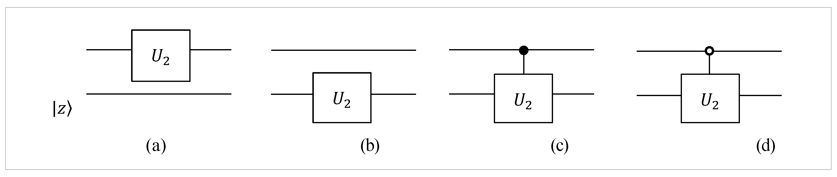
Figure 2.
The -point DsiHT by using the regular path.
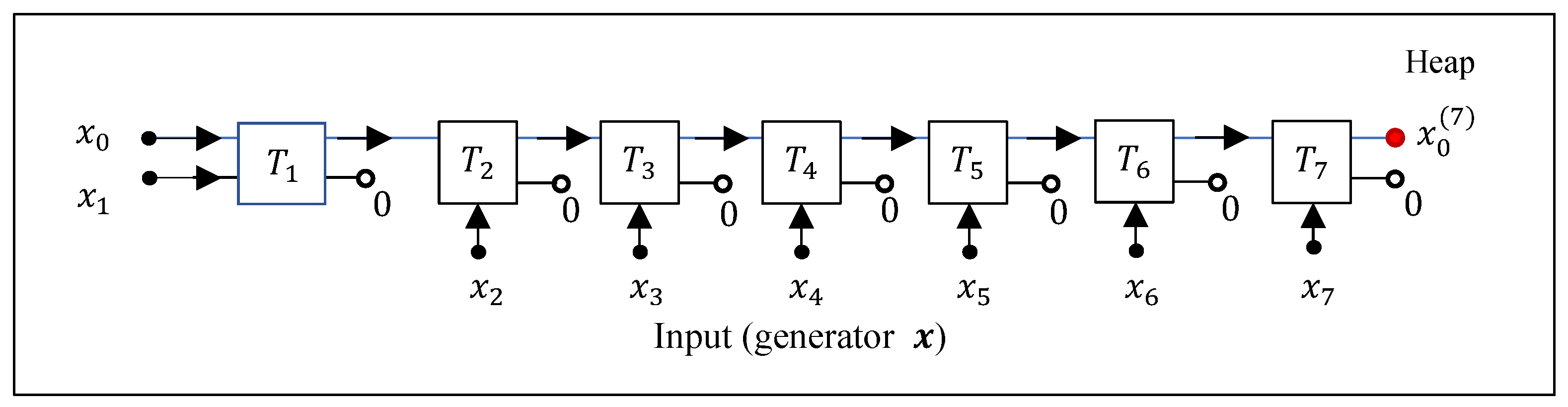
Figure 3.
The diagram of the -point weak 2-wheel carriage DsiHT applied to a signal .
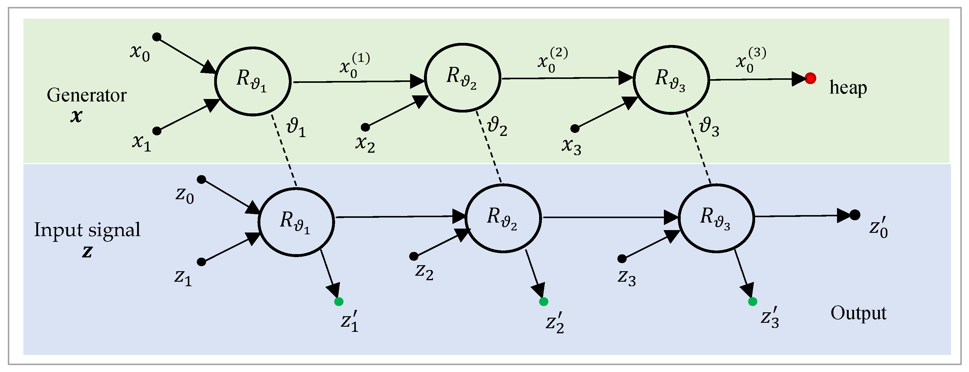
Figure 4.
The -point strong DsiHT on the generator.
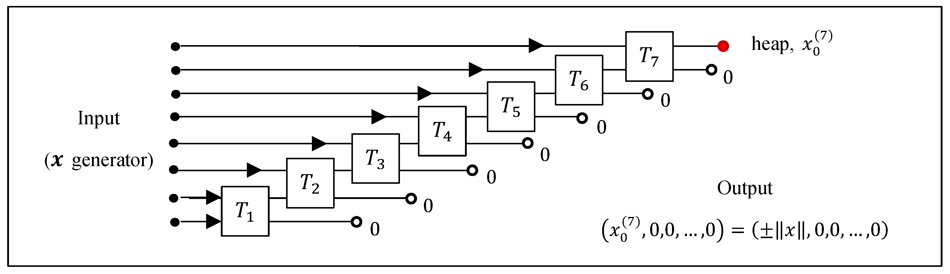
Figure 5.
The -point DsiHT (with the 2-wheel strong carriage).
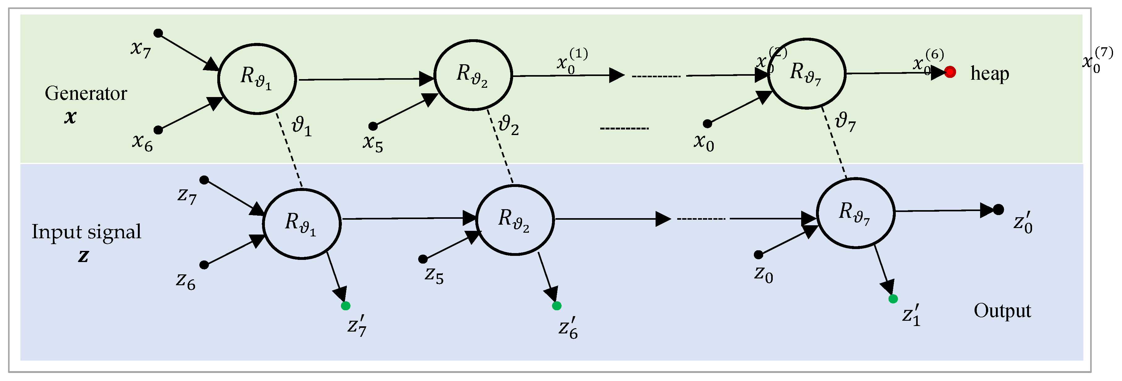
Figure 6.
The quantum scheme of the 2-qubit QsiHT with the generator .
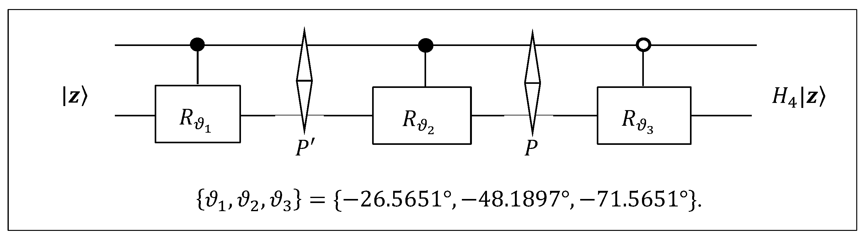
Figure 7.
The quantum scheme for initiation of the 2-qubit superposition by the 2-qubit inverse QsiHT.
Figure 7.
The quantum scheme for initiation of the 2-qubit superposition by the 2-qubit inverse QsiHT.
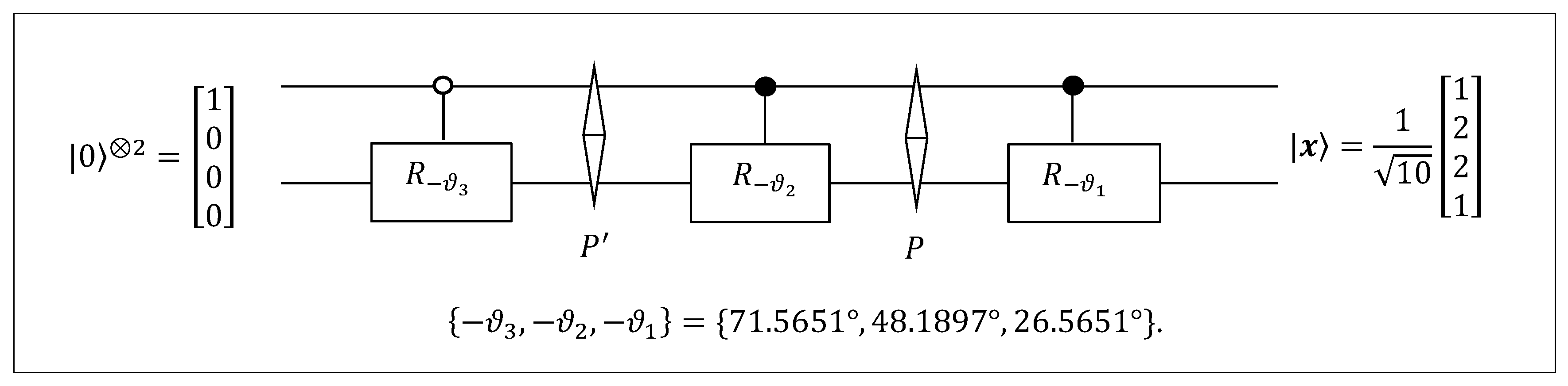
Figure 8.
The -point DsiHTs using two paths with splitting into pairs.
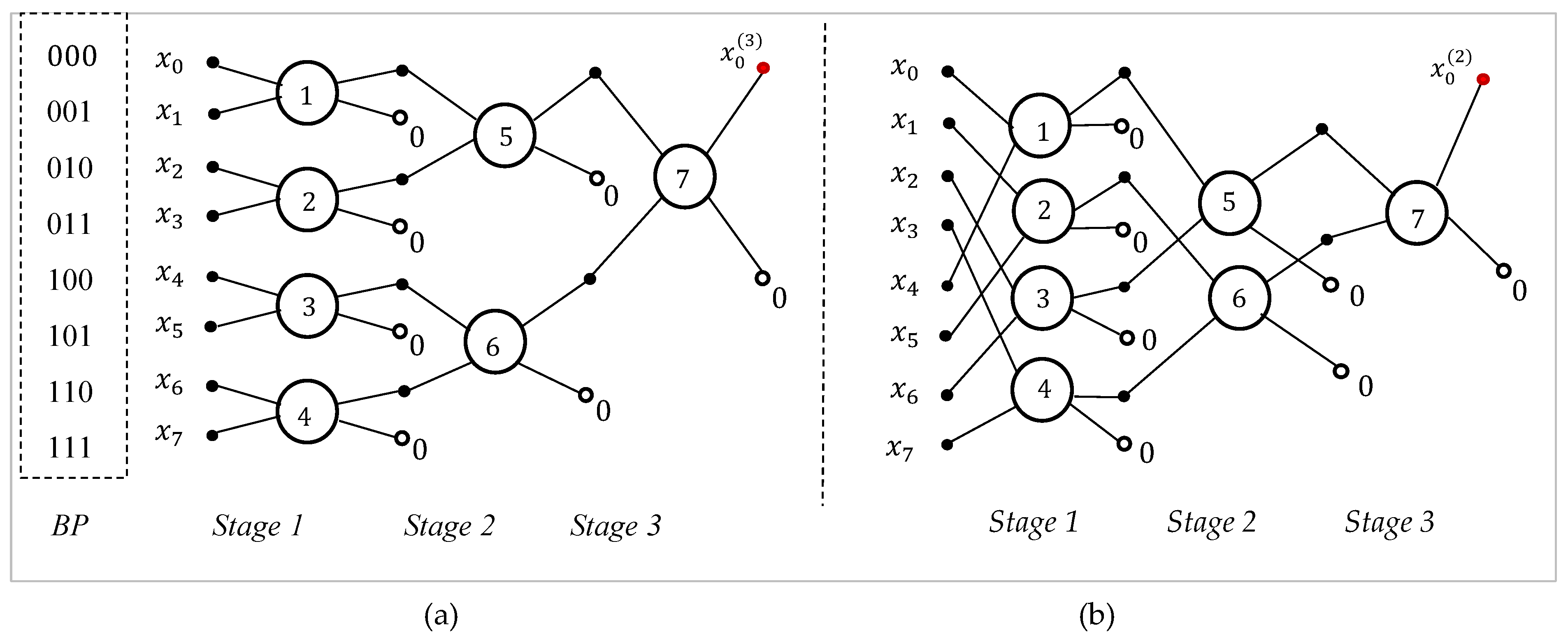
Figure 9.
Four 3-qubit rotation gates with two control bits.
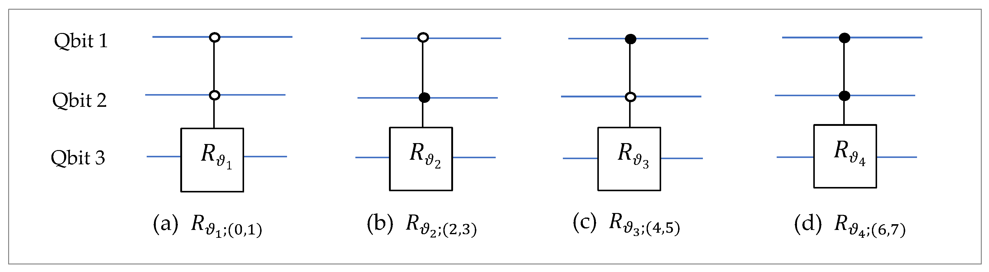
Figure 10.
Three 3-qubit gates with two control qubits in the second stage.
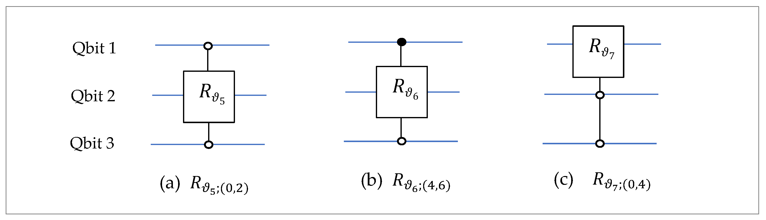
Figure 11.
The circuit for the 3-qubit QsiHT with seven controlled rotation gates.
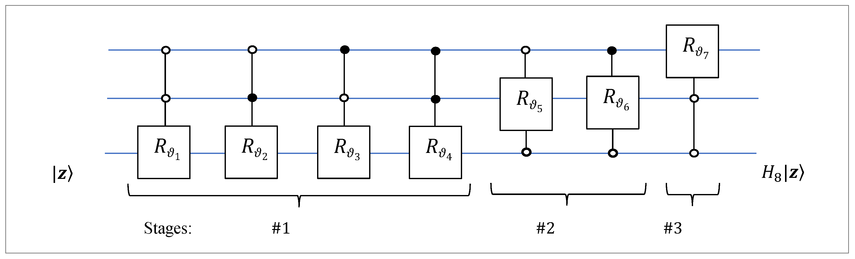
Figure 12.
The circuit for the inverse 3-qubit QsiHT with seven controlled rotation gates.
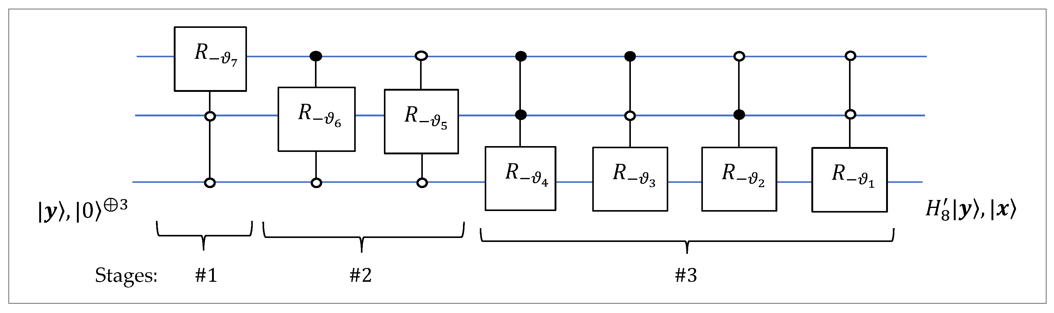
Figure 13.
The circuit for the initiation of the 3-qubit state
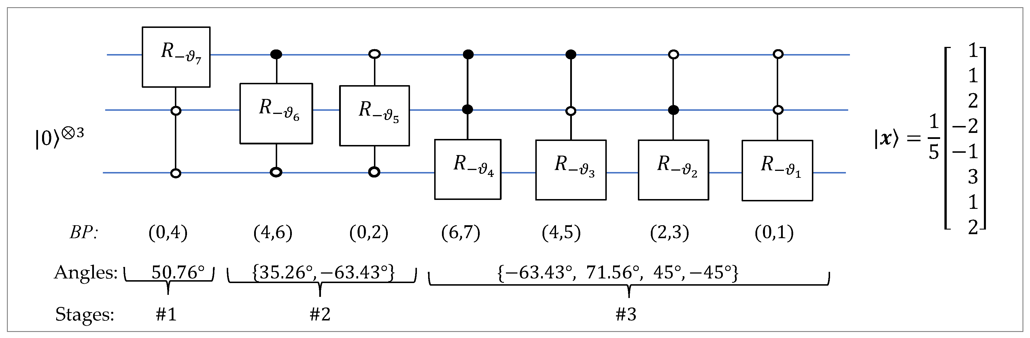
Figure 14.
The circuit for the 3-qubit QsiHT with seven rotations.
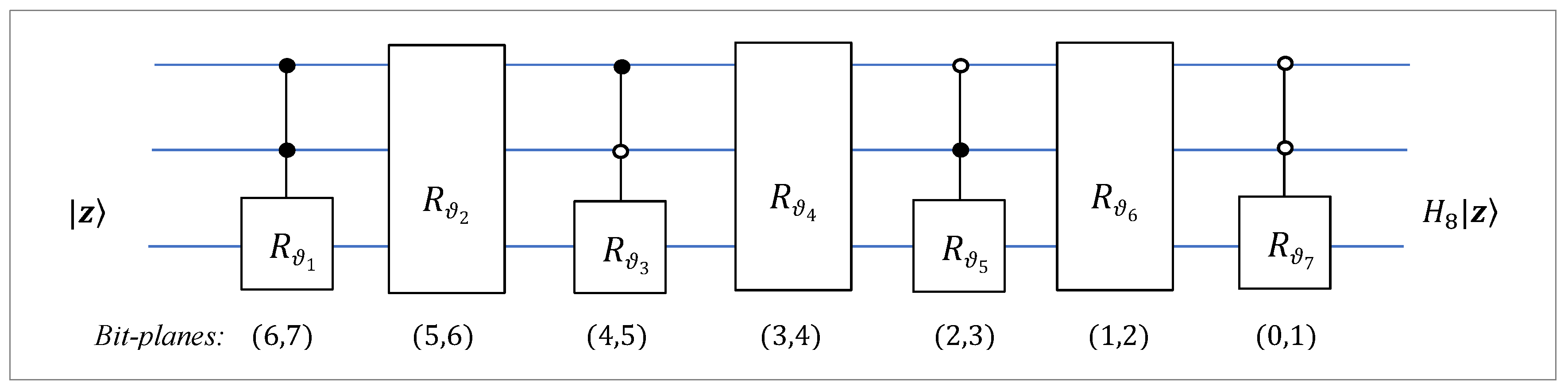
Figure 15.
The circuit for the 3-qubit rotation on the bit-planes 5 and 6 with two controlled NOTs.
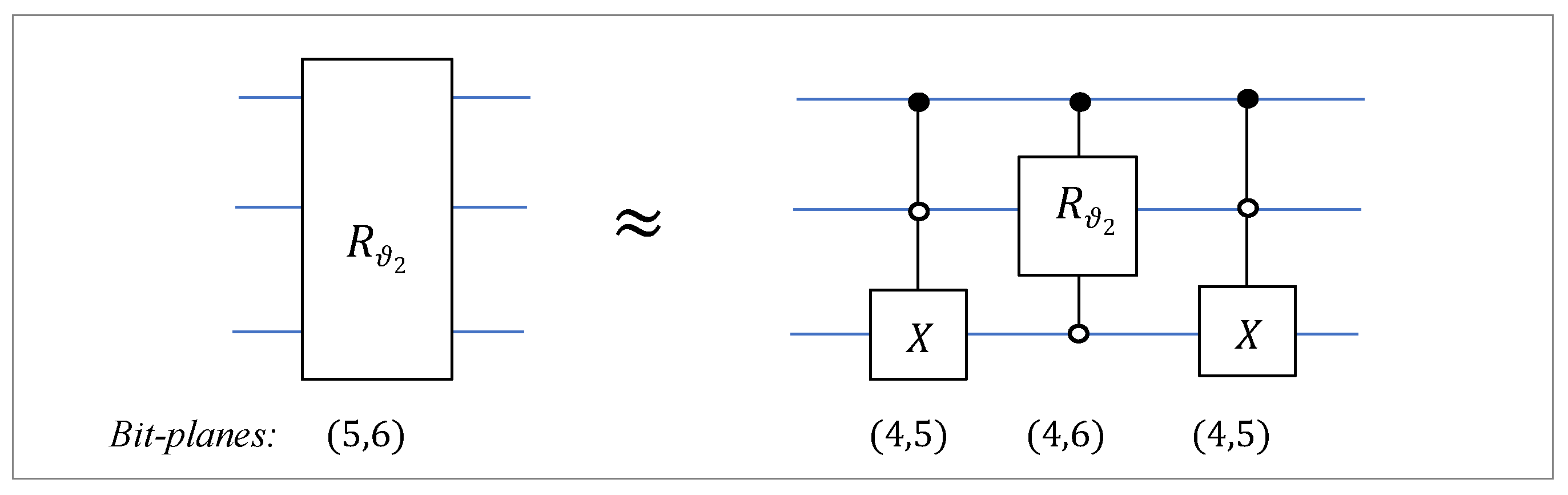
Figure 16.
The circuit for the 3-qubit rotation on the bit-planes 3 and 4 with four controlled NOTs.
Figure 16.
The circuit for the 3-qubit rotation on the bit-planes 3 and 4 with four controlled NOTs.
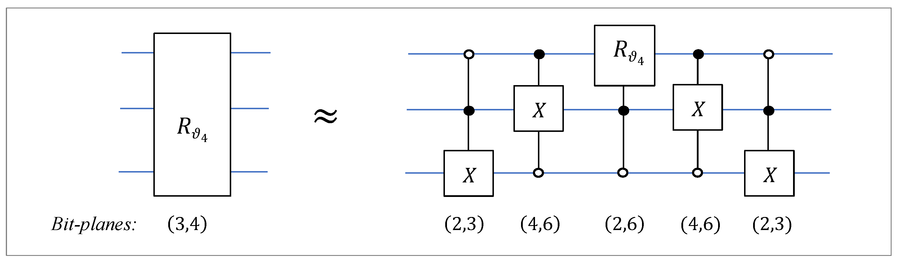
Figure 17.
The circuit for the 3-qubit rotation on the bit-planes 1 and 2 with two controlled NOTs.
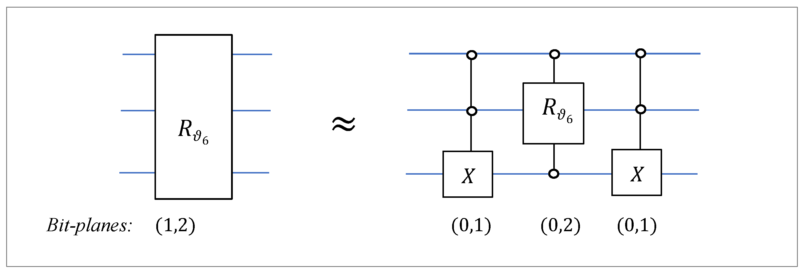
Figure 18.
The circuit for the 3-qubit strong QsiHT.
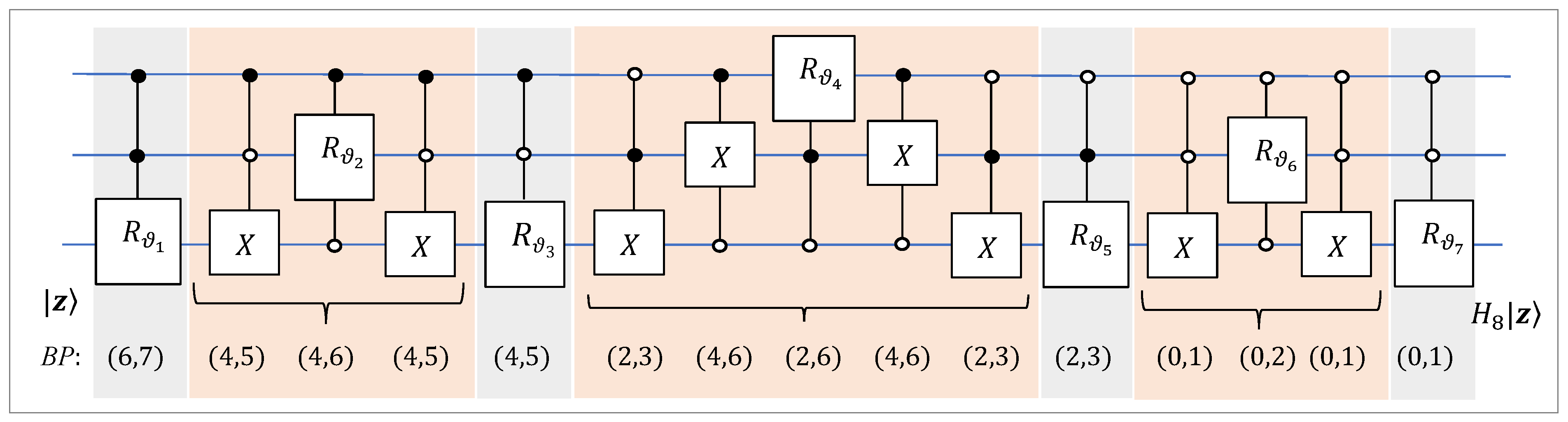
Figure 19.
The circuit for the inverse 3-qubit strong QsiHT.
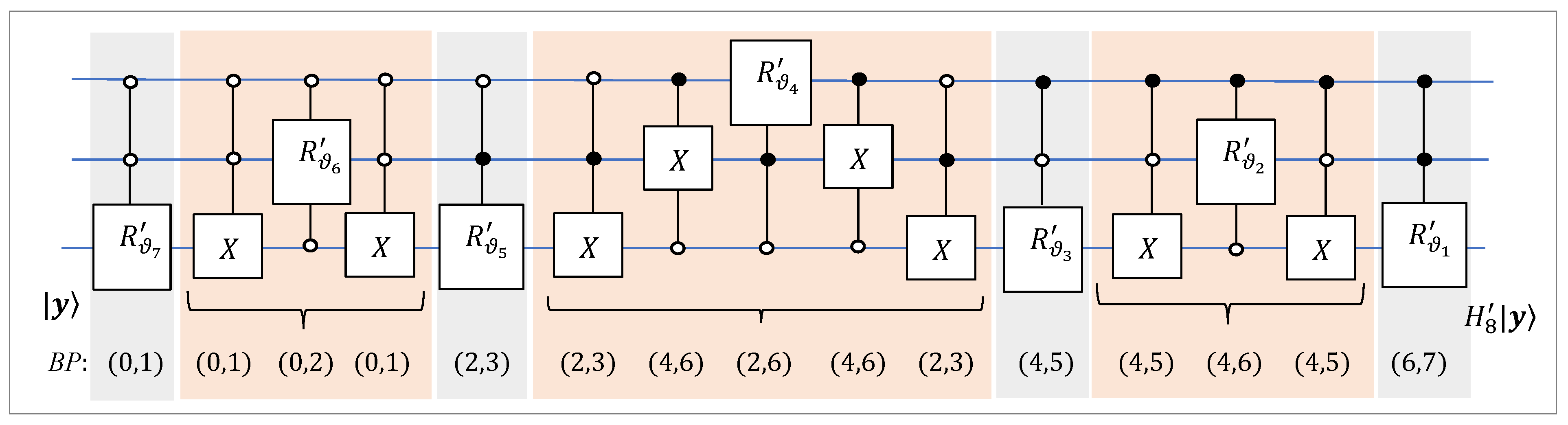
Figure 20.
The -point DsiHT using the path with splitting into pairs.
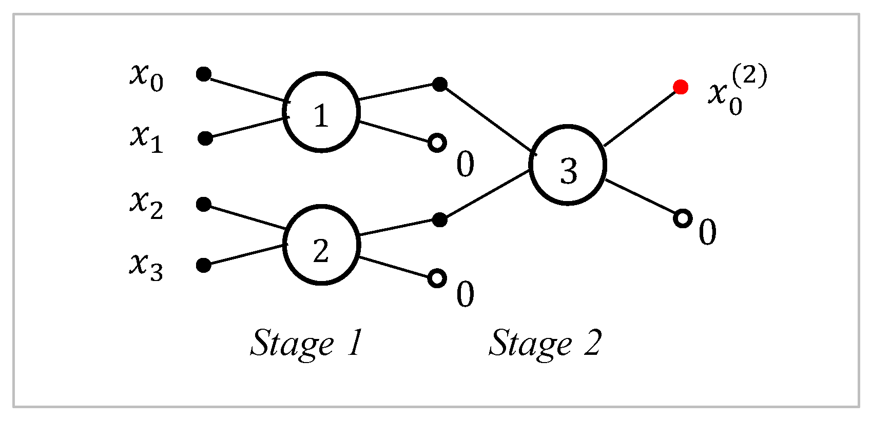
Figure 21.
The 2-qubit gates with control bit 0 or 1.
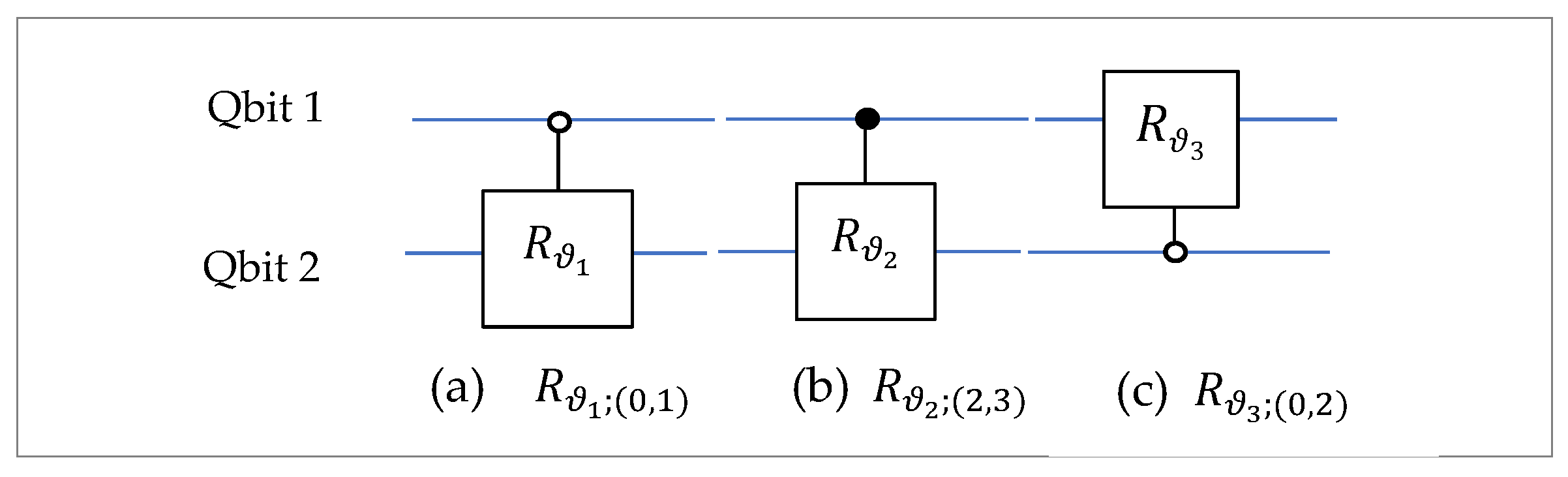
Figure 22.
The circuit for the inverse 2-qubit QsiHT with 3 controlled rotation gates.
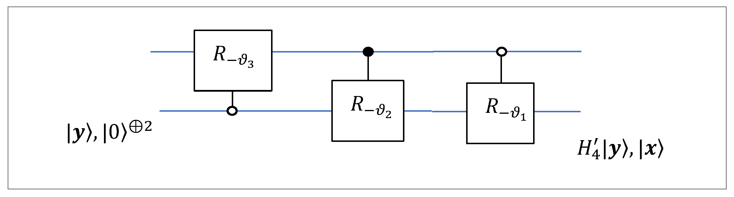
Figure 23.
The circuit for the initiation of the 2-qubit state .
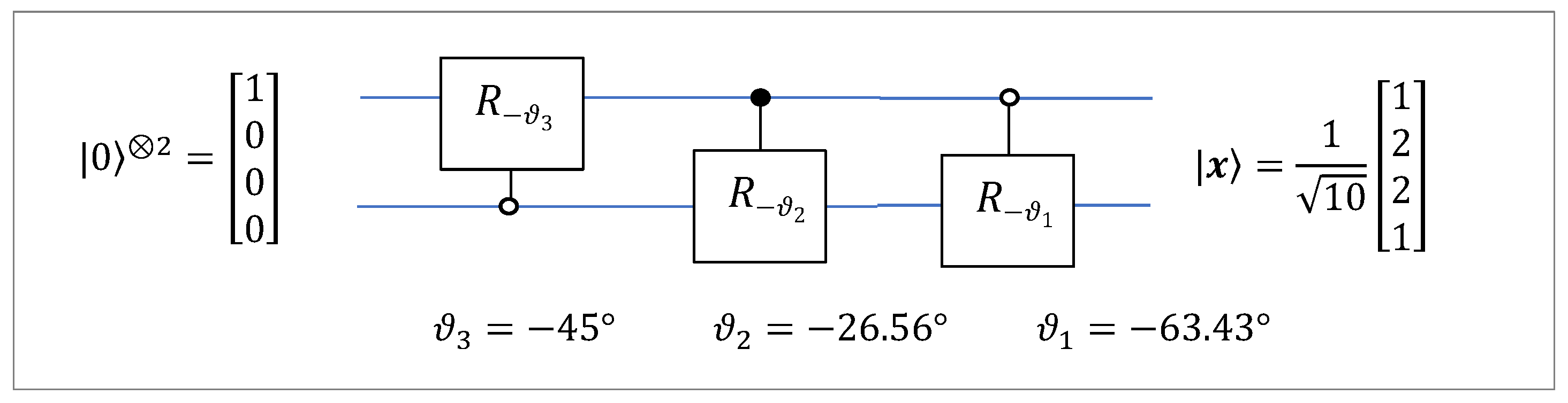
Figure 24.
The circuit for the initiation of the 2-qubit state from .
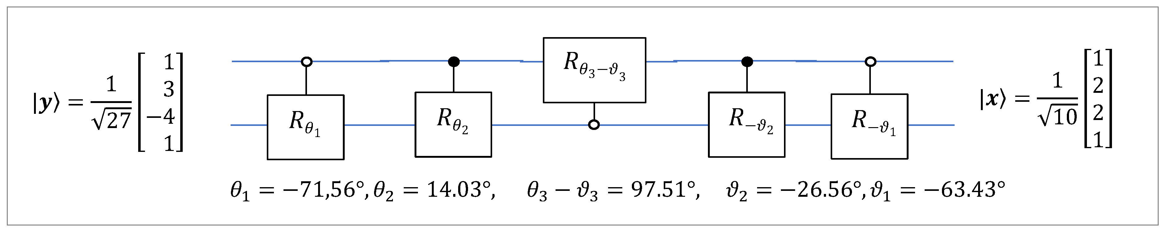
Figure 25.
The circuit for the 4-qubit QsiHT by the fast path #1.
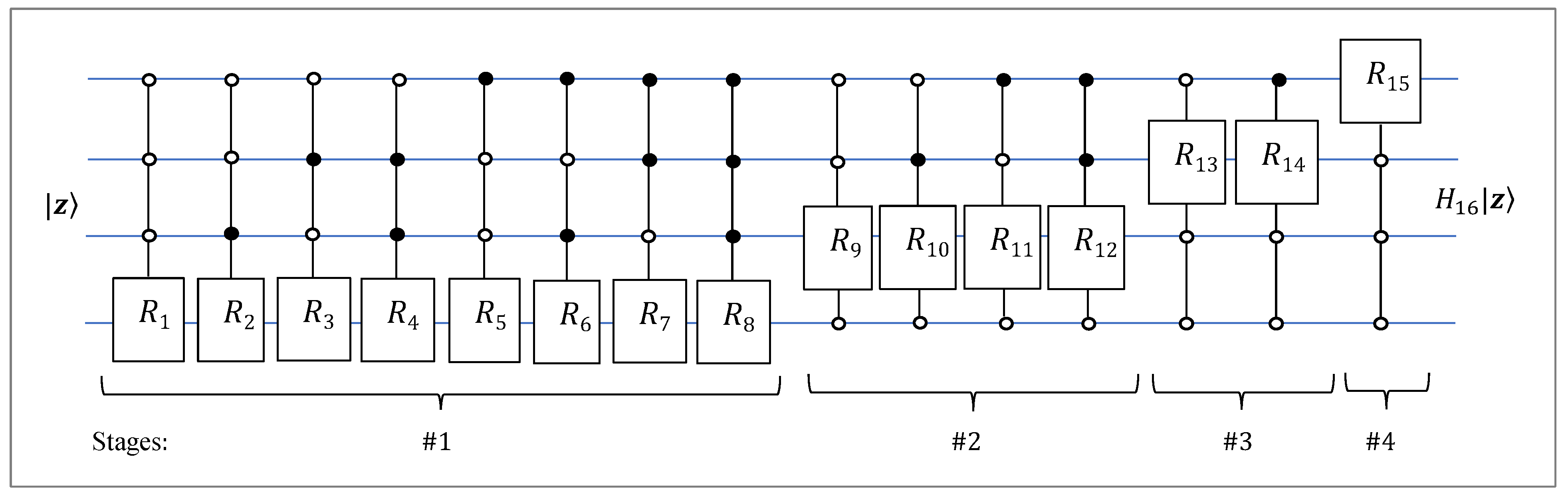
Figure 26.
The circuit for the 4-qubit inverse QsiHT by the fast path #1. (from: example7_paper.m).
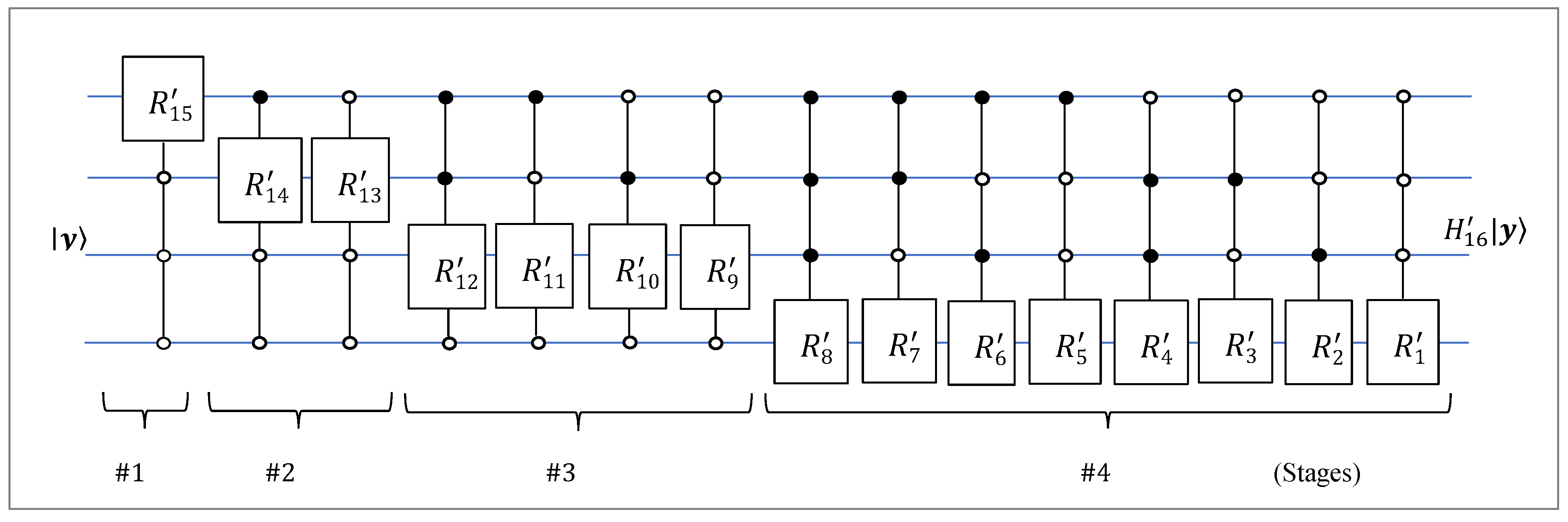
Figure 27.
The circuit for the 4-qubit QsiHT by the fast path #1.
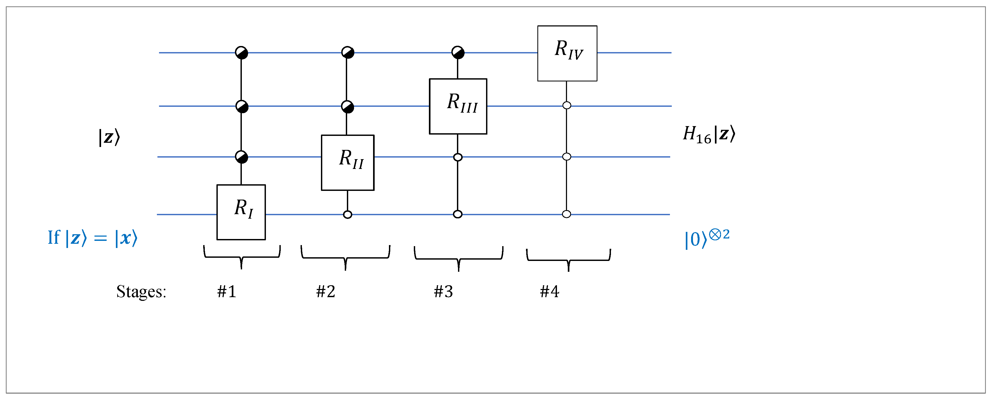
Figure 28.
The circuit for the inverse 4-qubit QsiHT by the fast path #1.
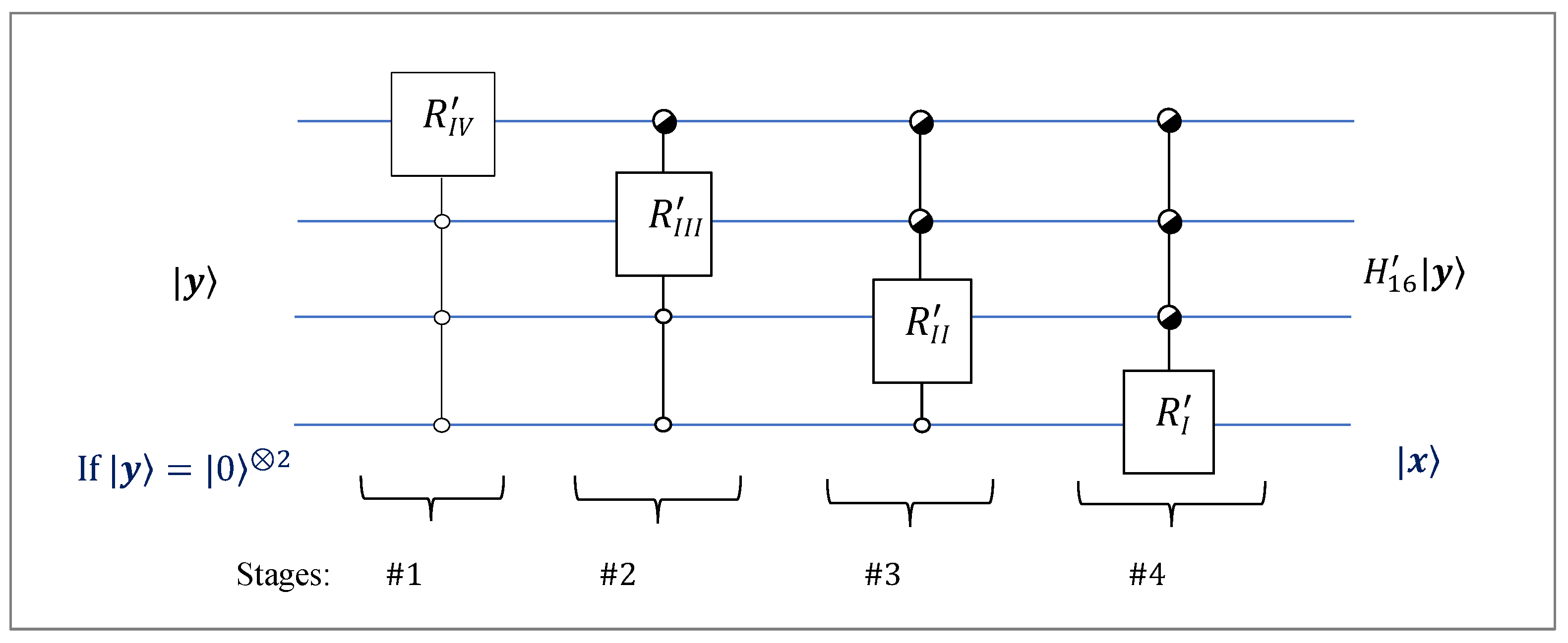
Figure 29.
The circuit for transforming one 4-qubit state into another, , by using two 4-qubit QsiHTs by the fast path #1.
Figure 29.
The circuit for transforming one 4-qubit state into another, , by using two 4-qubit QsiHTs by the fast path #1.
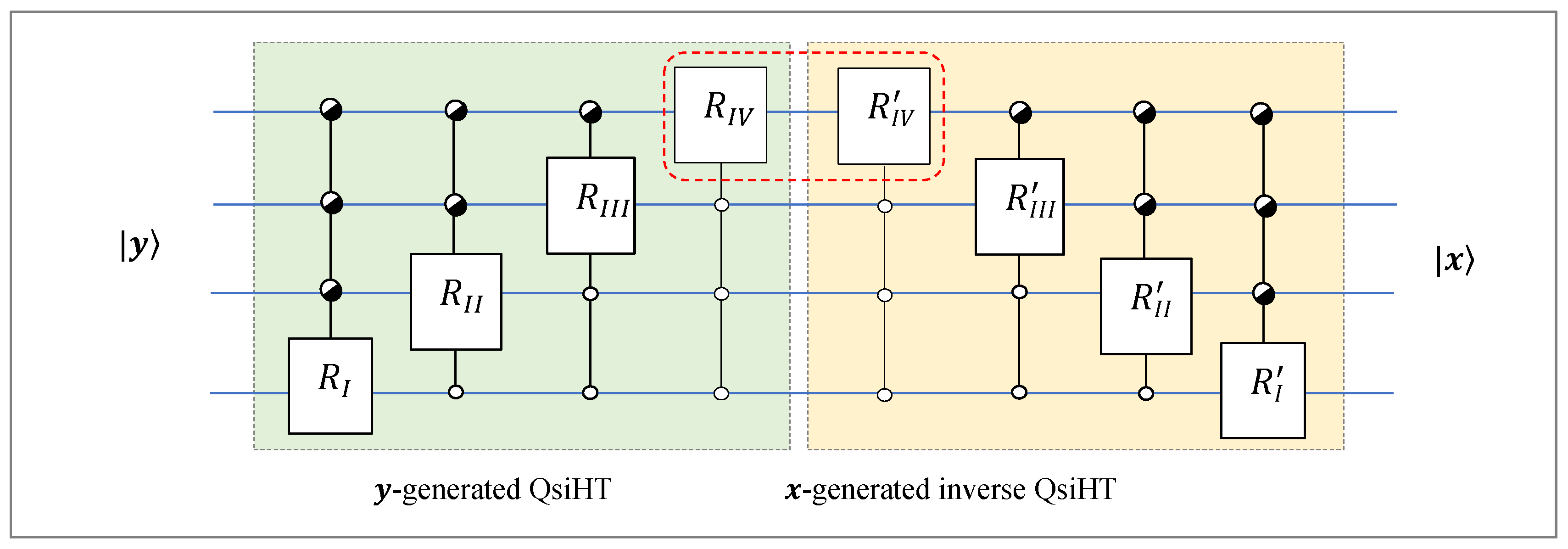
Figure 30.
The -point strong DsiHT with vector-parameter .
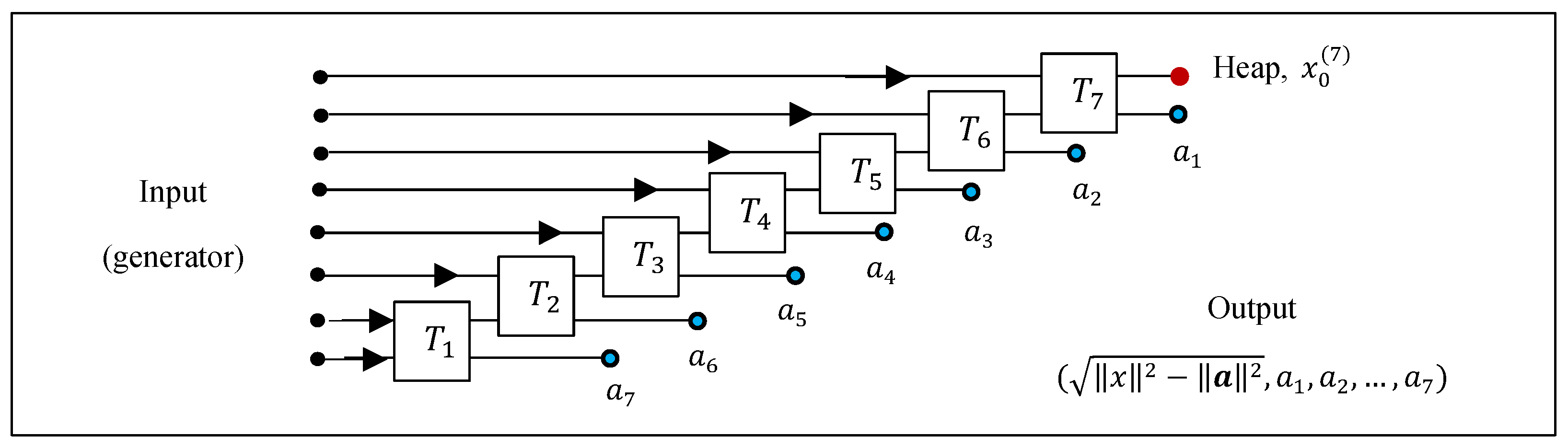
Figure 31.
(a) The 4-point DsiHT and (b) the 8-point DsiHT with the paths with splitting into pairs.
Figure 31.
(a) The 4-point DsiHT and (b) the 8-point DsiHT with the paths with splitting into pairs.
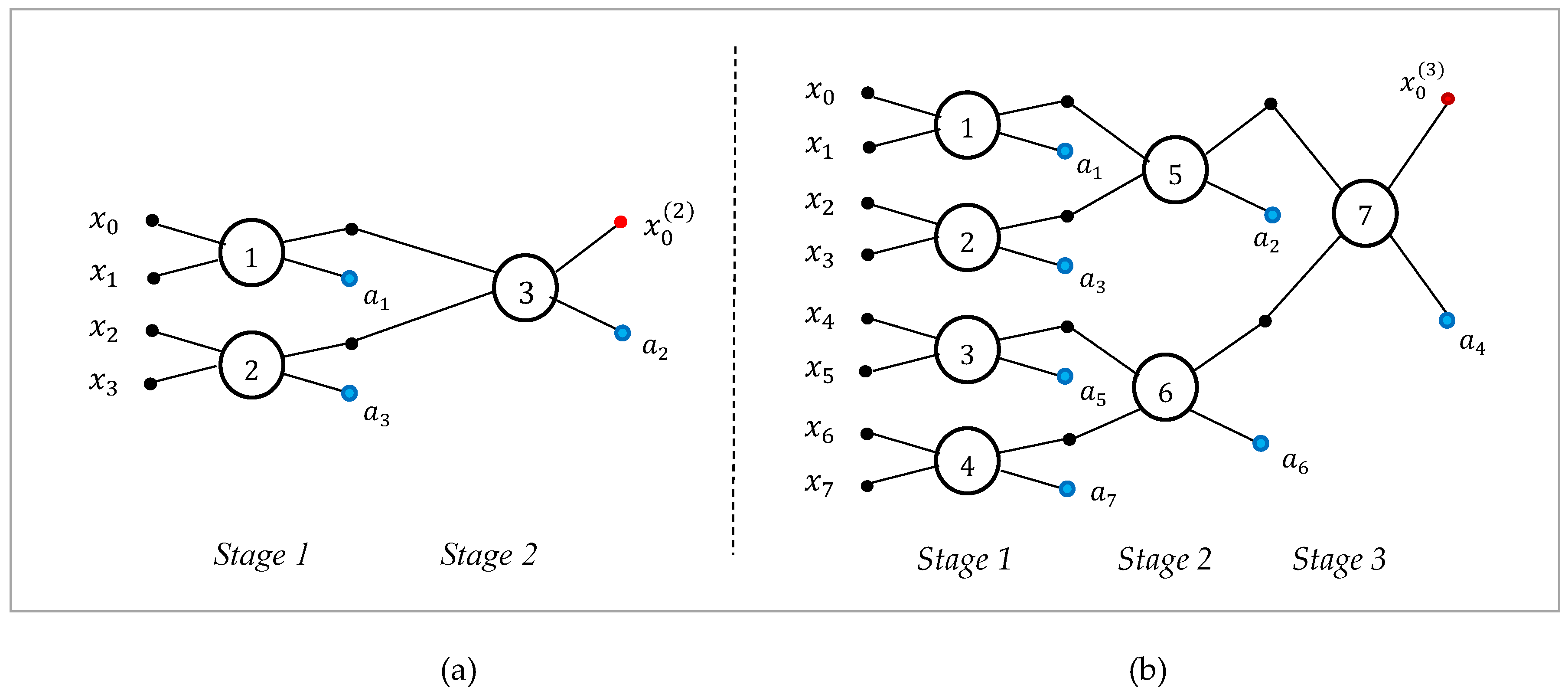
Figure 32.
The signal-flow graph of the -point DsiHT with the fast path.
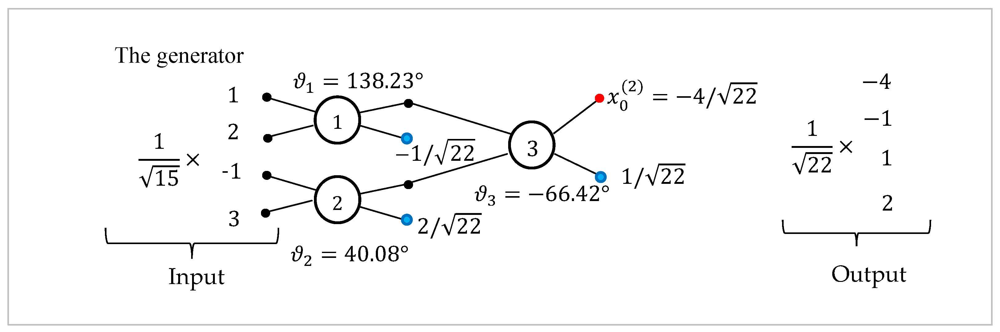
Figure 33.
The circuit for transforming the 2-qubit into the 2-qubit .
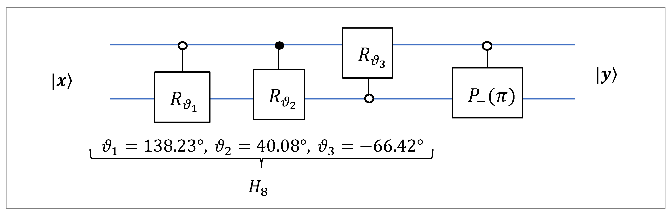
Figure 34.
The second signal-flow graph of the -point DsiHT.
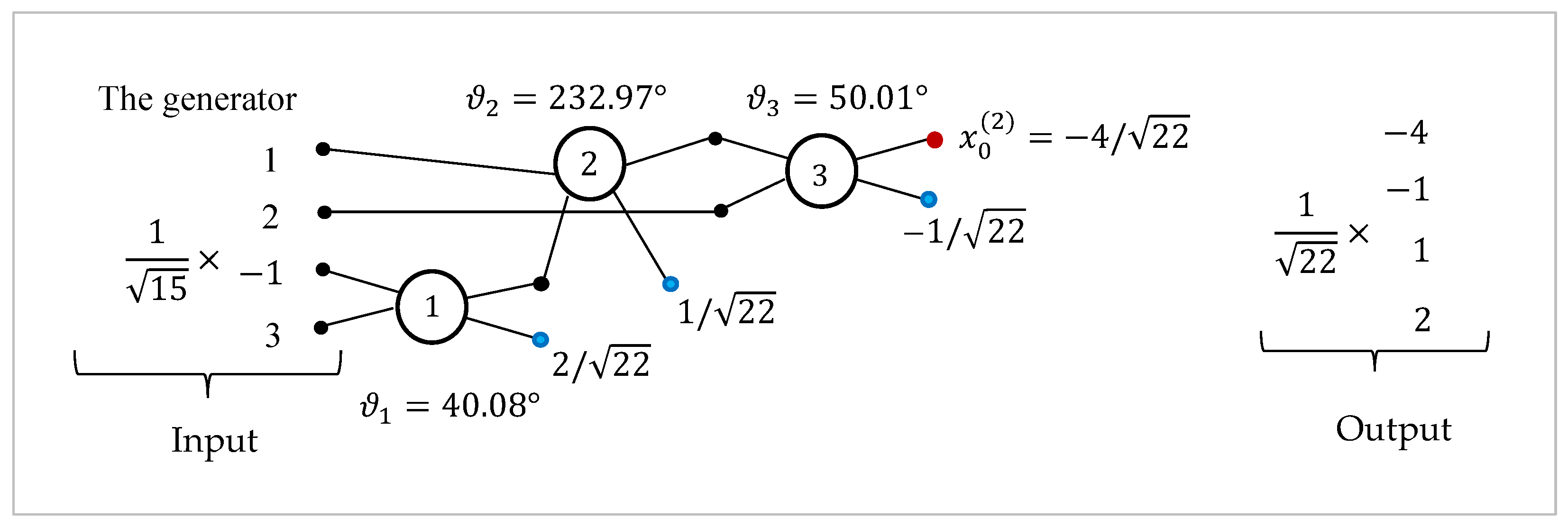
Figure 35.
The circuit for transforming the 2-qubit into the 2-qubit .
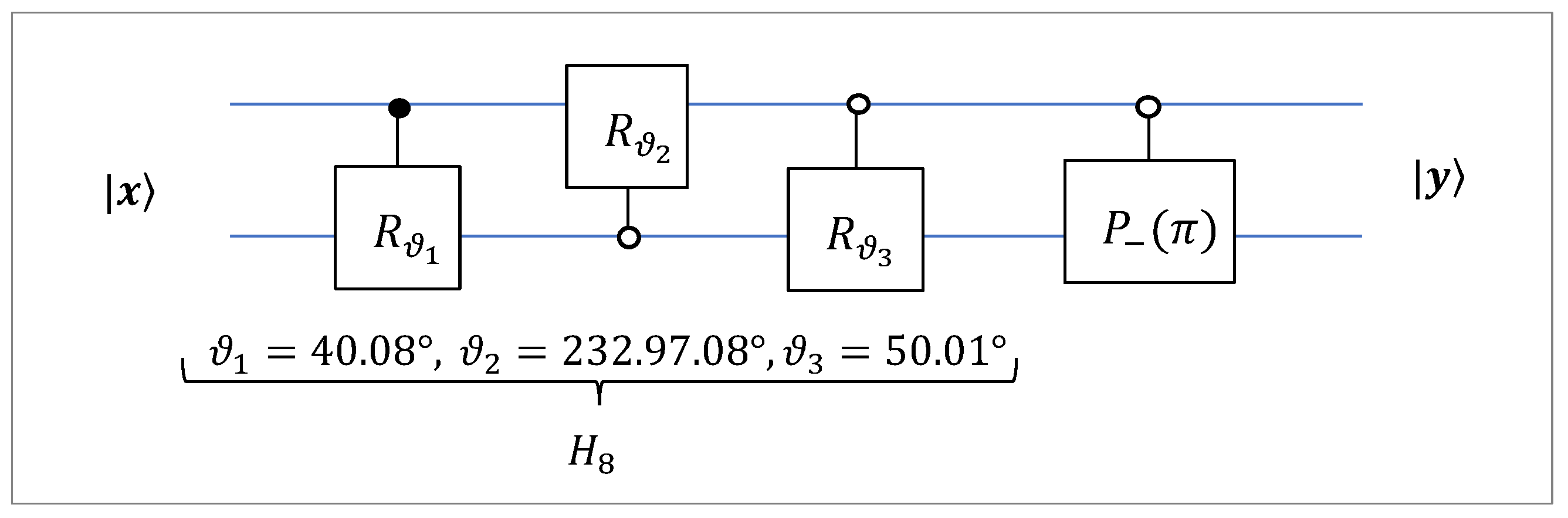
Figure 36.
The circuit for the 3-qubit transformation of states, .
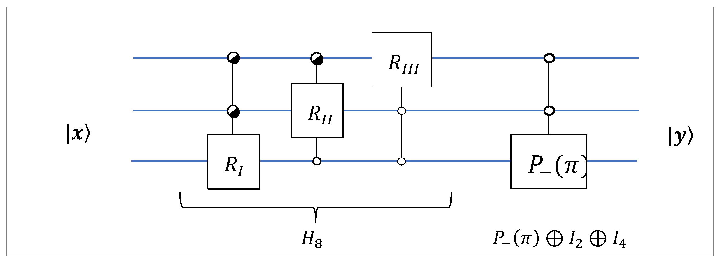

Table 1.
The measured magnitudes for 2-qubit superposition by the 2-qubit QsiHT.
| Basis States |
Magnitudes | ||||
| Theoretical | 500 shots | 1,000 shots | 10,000 shots | 100,000 shots | |
|
|
|
|
|
|
|
|
|
|
|
|
|
|
|
|
|
|
|
|
|
| MSRE |
|
|
|
|
|
Table 2.
The measured magnitudes of the 3-qubit state by the 3-qubit QsiHTs.
| Basis States |
Magnitudes | ||||
| Theoretical | Inverse strong QsiHT | Inverse fast QsiHT | |||
| 10,000 shots | 100,000 shots | 10,000 shots | 100,000 shots | ||
| 000 | 0.2000 | 0.1969 | 0.2005 | 0.2004 | 0.1989 |
| 001 | 0.2000 | 0.1978 | 0.1995 | 0.2008 | 0.2019 |
|
|
|
|
|
|
|
| 110 | 0.2000 | 0.2012 | 0.2007 | 0.2003 | 0.1995 |
| 111 | 0.4000 | 0.4012 | 0.3986 | 0.3982 | 0.3994 |
| MSRE |
|
|
|
|
|
Table 3.
Qiskit measured magnitudes for 2-qubit state by the 2-qubit QsiHTs.
| Basis States |
Magnitudes of |
||||
| Theoretical | Inverse strong QsiHT | Inverse fast QsiHT | |||
| 10,000 shots | 100,000 shots | 10,000 shots | 100,000 shots | ||
|
|
|
|
|
|
|
|
|
|
|
|
|
|
|
|
|
|
|
|
|
|
|
|
|
|
|
|
| MSRE |
|
|
|
|
|
Table 4.
Measured magnitudes for the 4-qubit through the DsiHT with the fast path.
| Basis States |
Magnitudes | ||||
| Theoretical | 500 shots | 1,000 shots | 10,000 shots | 100,000 shots | |
|
|
|
|
|
0.0936 |
|
|
1 |
|
|
|
|
|
|
|
|
|
|
|
|
|
|
|
|
|
|
|
|
|
|
|
|
|
|
| MSRE |
|
|
|
|
|
Table 5.
Measured magnitudes of the 2-qubit state after transferring the state .
| Basis States |
Magnitudes of |
|||
| Theoretical | 1,000 shots | 10,000 shots | 100,000 shots | |
|
|
|
|
|
|
|
|
|
|
|
|
|
|
|
|
|
|
|
|
|
|
|
|
| MSRE |
|
|
|
|
Table 6.
Measured magnitudes of the 3-qubit after state transformation .
| Basis States |
Magnitudes of |
|||
| Theoretical | 1,000 shots | 10,000 shots | 100,000 shots | |
|
|
|
|
|
|
|
|
|
|
|
|
|
|
|
|
|
|
|
|
|
|
|
|
|
|
|
|
|
|
| MSRE |
|
|
|
|
Disclaimer/Publisher’s Note: The statements, opinions and data contained in all publications are solely those of the individual author(s) and contributor(s) and not of MDPI and/or the editor(s). MDPI and/or the editor(s) disclaim responsibility for any injury to people or property resulting from any ideas, methods, instructions or products referred to in the content. |
© 2025 by the authors. Licensee MDPI, Basel, Switzerland. This article is an open access article distributed under the terms and conditions of the Creative Commons Attribution (CC BY) license (http://creativecommons.org/licenses/by/4.0/).
Copyright: This open access article is published under a Creative Commons CC BY 4.0 license, which permit the free download, distribution, and reuse, provided that the author and preprint are cited in any reuse.


