Submitted:
30 June 2025
Posted:
02 July 2025
You are already at the latest version
Abstract
In this study, we used the Hydrophobic-Polar (HP) two-dimensional square and three-dimensional cubic lattice models for the problem of Protein structure prediction (PSP). This kind of lattice reduces computational time and calculations, and the conformational space from 9n to 4n−2, even in this context, it is an appropriate benchmark problem for genetic algorithms. The contributions of the paper consist in: (1) implementation of a high-performing novel Genetic algorithm (GA); instead of considering only the self- avoiding walk (SAW) conformations approached in other work, we decided to allow any conformation to appear in the population at all stages of the proposed all conformations biomimetic Genetic Algorithm (ACGA). This increases the probability of achieving good native conformations (SAW ones), with the lowest energy that has the minimum number of contacts in the lattice, the one with the maximum topological neighbors. In addition to classical crossover and mutation operators, (2) we introduced specific translation operators for these two operations. We have proposed and implemented an HP Protein Visualizer tool which offers interpretability, a hybrid approach in that the visualizer give some insight to the algorithm, that analyse and optimise protein structures HP model. The program resulted based on performed research, provides a molecular modeling tool for studying protein folding using technologies such as React, Next.js, and Three.js for 3D rendering, and includes optimization algorithms to simulate protein folding.
Keywords:
Biomimetic Genetic algorithm use with interpretability
; Benchmark problem for generic algorithms
; Protein structure prediction
; Lattice model
; Combinatorial optimization
; Representation
; Stochastic optimization
; Visualisation
1. Introduction
The molecular structure of a protein can be broken down hierarchically into four levels. The protein’s primary structure is its sequence of amino acids (AAs), the secondary structure is its locally folding pattern, the tertiary structure is the globally folded form, frequently as a globule, and its quaternary structure is its multimeric organization [1].
Protein folding (PF) is the physical process by which a protein chain is translated into its native three-dimensional (3D) structure, typically a “folded” conformation in which the protein becomes biologically functional. This process is fundamental because only in a good tertiary structure (native conformation) can the protein become biologically functional [2].
The algorithms must predict the correct native conformation and the purpose of PSP is to predict the tertiary structure from the primary structure. Due to its extreme complexity, several simplified protein models have been proposed, reducing the algorithms’ search space. Three approaches can be classified: 1) de novo (ab initio) starting only from the information contained in the primary structure of the proteins, 2) homology – using information from the primary structure and knowledge of the native conformations of similar sequences, and 3) protein threading (or fold recognition), using knowledge of the fold families [3,4].
The fundamental motivations of this work are:
(1) Complexity of protein modelling. Understanding protein structures is crucial to revealing biological functions and diseases associated with protein misfolding, such as Alzheimer’s disease [5]. The HP model provides a simplified yet robust framework for examining the basic principles of protein folding without the need for extensive computational resources.
(2) Lack of accessible tools. Most existing tools, such as Rosetta [6] or GROMACS [7], require advanced programming knowledge and are difficult to use.
The main objective of this work was to provide researchers, students, and bioinformatics professionals to explore protein folding visually in three-dimensional space. Through its interface, HP Protein Visualizer understanding of the relationship between amino acid sequences and resulting 3D structures—an essential aspect of protein study and its applications in biotechnology and medicine.
Contribution to PSP. This paper describes a new biomimetic Genetic algorithm used for solving PSP on the HP model. The algorithm considers, at all stages, populations formed of all configurations, without excluding the invalid (unfeasible) ones. A conformation is valid (feasible) if and only if it respects the self-avoiding walk (SAW) condition, which means that no two beads (i.e., amino acids represented as nodes placed on a 2D or 3D lattice) are placed in the same position on the lattice (thus avoiding overlaps).
Allowing invalid configurations in the populations is beneficial due to the chaotic behavior of the associated energy, increasing the chances of finding good partial solutions (valid configurations) generated through small changes applied to some invalid configurations.
Furthermore, the original approach includes, in addition to classical crossover (rotational) and mutation (rotational and diagonal) operators, the application of translation operators for both crossover and mutation operations.
An important and novel aspect of this work lies in the hybrid integration between the ACGA and the HP Protein Visualizer. The visual component offers interpretability of how genetic operators influence protein geometry and provides an interface for debugging, hypothesis testing, and exploratory purposes.
The remainder of the paper is organized as follows: Section 2 presents the related work in the domain of PSP, followed by Section 3, which describes the HP model and the PSP within heuristic techniques. Section 4 presents the hybrid algorithms, while section 5 presents and analyzes the results obtained by applying the proposed algorithms to a set of popular benchmarks. Finally, section 6 and section 7 offer a conclusive analysis of the results and future work.
2. Related Work
According to the thermodynamic hypothesis [8], the native conformation is determined solely by the protein’s AAs sequence, and in this conformation, the protein reaches its minimum free energy. Even if a given protein has only one native conformation (the correct conformation), it can still fold into a multitude of other conformations, which are erroneous.
Simulated annealing (SA) and genetic algorithm (GA) were applied by Unger [9], Custodio [10], Jiang [11] and Cox [12,13]; the evolutionary Monte Carlo (EMC) method applies Liang and Wong [14].
Zhou et al [15] present a combination of particle swarm optimization (PSO) and tabu search (TS) to the PSP, using the 3D HP lattice model, and Huang applied GA-based on Optimal Secondary Structures (GAOSS) on the 2D HP model [16].
In a previous study [17], Benitez et al. applied a hybridization of the parallel artificial bee colony (ABC) and GA to the 3D HP model with side chains to solve PSP on the Beowulf cluster.
Rashid et al. [18], evaluated different algorithms, including the Local Search (SS-Tabu), GA, and hybrid algorithms (Hybrid GA), on the five benchmark sequences. However, their algorithms performed poorly on large proteins (sequences with lengths greater than 100 AAs). In another study [3], the authors used the single-point crossover genetic operator and mutation with rotation and diagonal-pull-tilt moves. Additionally, in a different study [19], the authors created a multithreaded local search framework (SS-Parallel) that allowed all threads to execute the spiral search (SS-Tabu) and GA (selections and random-walk).
Over time, several models have been proposed to predict protein structures and explain the folding process. A very simple but efficient model is the HP model, which was proposed by Dill [20] and further developed in the following years [21]. PSP on this model belongs to the ab initio methods, where the proteins are represented as sequences of hydrophobic or non-polar (H), and hydrophilic or polar (P) characters arranged on a 2D or 3D lattice. The goal is to find a conformation that minimises the energy, typically defined by the number of non-consecutive H-H contacts.
In the study of [22], a mathematical model for the HP triangular lattice was applied to a GA, obtaining good results on small sequences. More recently, the authors [23] applied a GA on the 2D HP model on larger sequences (50 to 100 AAs), but the optimum energy was not attained [23].
The HP model uses a discretized space (lattice), where the amino acids (AAs) of the protein sequence are placed on the lattice nodes. The conformations are determined by the positions of the AAs, and they are differentiated by introducing a free-energy function, which is a score determined by these positions and not by the thermodynamic free energy [24,25]. However, even with this discretization, an exhaustive search is not feasible as PSP on this model has been proven to be an NP-complete problem [26].
To solve PSP on the HP model, heuristic techniques from different classes, such as Machine Learning (ML) [27], evolutionary algorithms (EA) [28,29], GA [2], and Monte-Carlo (MC) simulations have been applied. PSP on the HP model requires combinatorial chromosome encoding, and the energy function expresses chaotic behavior in the Devaney sense [30,31]. That is why the GA applied to PSP has issues with convergence and reaching the optimum.
Comparison with AlphaFold and RoseTTAFold. Recent advances in deep learning have revolutionised protein structure prediction. AlphaFold [32], developed by DeepMind, has achieved unprecedented accuracy in predicting protein 3D structures from amino acid sequences. It uses a transformer-based neural network architecture trained on protein structures and sequences. AlphaFold [33] demonstrated near-experimental accuracy in the CASP14 challenge, making it a groundbreaking development in structural bioinformatics.
RoseTTAFold [34], developed by the Baker lab, is another deep learning-based method for protein structure prediction [35]. It uses a three-track network that considers sequences, distance maps, and coordinates simultaneously. RoseTTAFold is open-source and has been used for applications beyond structure prediction, including docking and design.
The ab initio is important since it gives meaning to PF, but it has not yet been completely solved. Therefore, our focus is on this ab initio variant. From a computational standpoint, the ab initio variant of the HP model addresses the Protein Structure Prediction (PSP) problem as a combinatorial optimization task in a discrete search space , where each conformation corresponds to a self-avoiding walk (SAW) on a 2D or 3D lattice. The objective function computes the energy of a structure based on hydrophobic (H-H) contacts, and the goal is to find the minimum energy structure:
Unlike AlphaFold or RosettaFold, which rely on probabilistic models trained on large biological datasets and perform inference in high-dimensional continuous spaces, the ab initio HP model operates without external information, learning, or evolutionary alignments. It explores a rugged, high-dimensional, discrete landscape where exact methods are infeasible due to NP-completeness.
Therefore, heuristic and metaheuristic approaches, such as genetic algorithms [36], are essential for navigating the vast configuration space.
There were some state-of-the-art GAs developed in the scientific literature for the HP lattice model, primarily focusing on sequence optimization and folding energy minimization. In this context, the development of a biomimetic hybrid Genetic algorithm is used with visualization tools to ensure interpretability, enabling dynamic evaluation of folding configurations, parameter control, augmented by local move operators and guided by visual heuristics.
3. Heuristic Techniques
PSP on the HP model involves three stages: (1) choosing a suitable type of lattice (e.g., 2D-square, 2D-trigonal, 2D-rectangular, 3D-cubic, 3D-Face-Centered Cubic); suitability is defined either by the appropriateness to the structure of real proteins or by the higher probability to reach a solution; 2) choosing an arbitrary energy function to model the protein conformation on the lattice, making it similar to the real protein’s native conformation (i.e., forming the hydrophobic kernel/kernels and the polar surface); and (3) creating a new algorithm or modifying an existing one that can solve the protein folding problem in this lattice-based setting.
Two AAs placed on adjacent nodes in the lattice can be either sequence neighbors or topological neighbors. Sequence neighbors are neighbors in the protein’s primary structure, while topological neighbors are positioned on nearby nodes to form contacts.
The arbitrary energy function should be defined to maximize the number of contacts between hydrophobic AAs. This can be achieved by assigning a value of free energy for each type of contact, as follows: ; ; ; . Specifically, H-H contacts are encouraged, while other types of contacts are neither encouraged nor penalized. An H-H contact between the and AA from the original sequence can be formed only if . Based on these criteria, the free-energy, E, of a conformation c is calculated as the sum of H-H contacts, taken with the minus sign (see Equation 2):
The negation is applied to ensure similarity with thermodynamic free energy.
For the basic HP model, PSP problems on square lattices have been proved to be NP-complete problems by Crescenzi [37] and Berger [26]. Based on these results, it has been concluded that all other problems on more general lattices and on tree-dimensional ones are also NP-complete.
Problem definition. For computational reasons, a more formal and general definition of the k-dimensional problem is needed:
Let be a geometrical lattice in and be a string of H and P letters ().
- The lattice is defined by:
where form a base of a vector space .
For the 2D square lattice () and 3D cubic lattice (), the vectors ... have to satisfy the following two conditions : 1) , and 2) .
The string represents an AAs sequence in the HP model, where H corresponds to a hydrophobic AA, and P corresponds to a polar AA. To simplify the explanation, we refer to the modeled AAs as “beads.” In the sequence, each bead has exactly two neighbors, except for the first and last beads, which have only one neighbor (successor and predecessor, respectively). The distance between any two neighboring beads is equal to 1.
Conformations. A conformation is defined by the placement of the string on the lattice. The placement must adhere to the following restrictions: 1) only one bead can be placed in each position on the lattice; 2) the string cannot be broken; neighboring beads in the string should be placed in neighboring positions in the lattice.
A conformation corresponds to a walk in the lattice, representing the placement of the string on it. A conformation is feasible if and only if respects self-avoiding walk (SAW) condition, which means that no two beads are placed in the same position on the lattice.
There are two common types of encodings used to represent a conformation. These encodings specify directions to follow the walk. In the first type, known as absolute encoding, the fold directions are relative to the lattice. In the second type, known as relative encoding, the fold directions are relative to the conformation itself.
- For the 2D square lattice, the two encodings are denoted as follows:
- string – for absolute encoding, where R stands for right, L for left, U for up, and D for down;
- string – for relative encoding, where S stands for straight, R for right, and L for left.
- For the 3D cubic lattice, the two encodings are denoted as follows:
- string – for absolute encoding, where R stands for right, L for left, U for up, D for down, F for front, and B for back;
- string – for relative encoding, where S stands for straight, R for right, L for left, F for front, and B for back.
The free energy of a conformation is calculated based on the Equation 2. Free energy of a conformation is a function depending on the HP-string, the encoding-string, and the lattice-type, as can be seen in Equation 4.
Problem requirement. For a given sequence (HP string), find the optimal configuration for which the free-energy is minimal [38]. This implies that the H beads are positioned in the center of the lattice, and this configuration should directly correlate with the native configuration of the real protein.
Therefore, the problem is a combinatorial optimization one [39,40], which can be solved using either deterministic or nondeterministic algorithms. In this case, we have chosen nondeterministic GA.
For all the cases, the problem input is the string that represents the unfolded string of beads (Example: HPHPPHHPHPPHPHHPPHPH).
The output of the algorithm depends on the lattice type. For example, in the two-dimensional case, the output could be the string (or string), representing the folded string with the minimal energy configuration that satisfies the SAW condition.
The objective function is defined by the energy equation (Equation 2).
4. Optimisation Algorithms
Three different optimization techniques are used to find protein conformations with the lowest amount of energy.
4.1. Monte Carlo Simulation
MC simulation is a stochastic method that explores the conformational space through random sampling. It applies the Metropolis criterion [41] to decide whether to accept or reject a structural mutation based on energy change. Our implementation includes custom move sets, such as corner flips, crankshaft motions, and pivot moves. The system was evaluated with 1000 iterations and a constant temperature of 1.0, which probabilistically accepts structural mutations that increase the system’s energy, according to:
Figure 1.
Monte Carlo Interface. Folding Trajectory
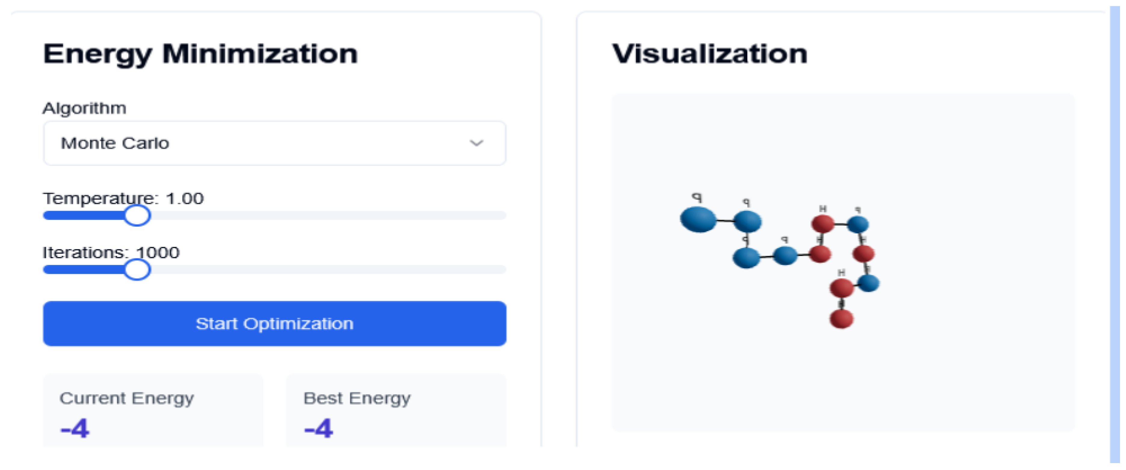
where is the energy difference and T is the temperature.
Figure 2.
MC Energy evolution
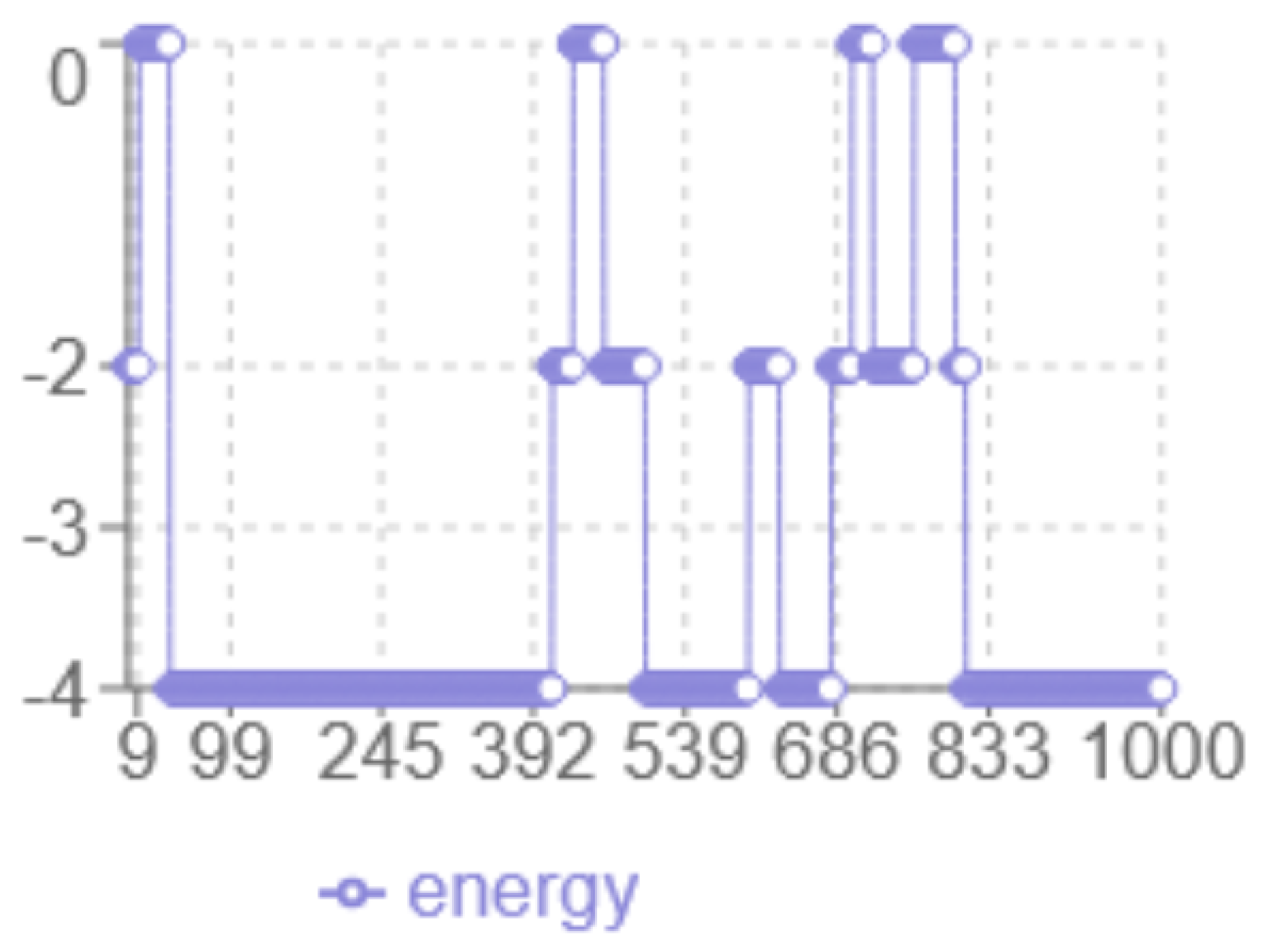
The analysis of the energy profile in 2 reveals the following characteristics: the x-axis corresponds to the iteration number, while the y-axis represents the energy level multiplied by two. The minimum energy achieved is , representing the best result among the tested methods. The algorithm displays a dynamic behaviour with significant fluctuations between 0 and -4, indicating more in-depth exploration of the solution space, with abrupt transitions that indicate the algorithm’s ability to escape local optima. The final structure has multiple hydrophobic (H-H) interactions at the minimum energy level.
4.2. Simulated Annealing
SA extends the Monte Carlo approach by progressively lowering the temperature to reduce the acceptance probability of less optimal moves [42]. This mimics the annealing process in metallurgy. We use exponential cooling and adaptive temperature steps based on energy fluctuations.
Figure 3.
Conformational changes SA Interface
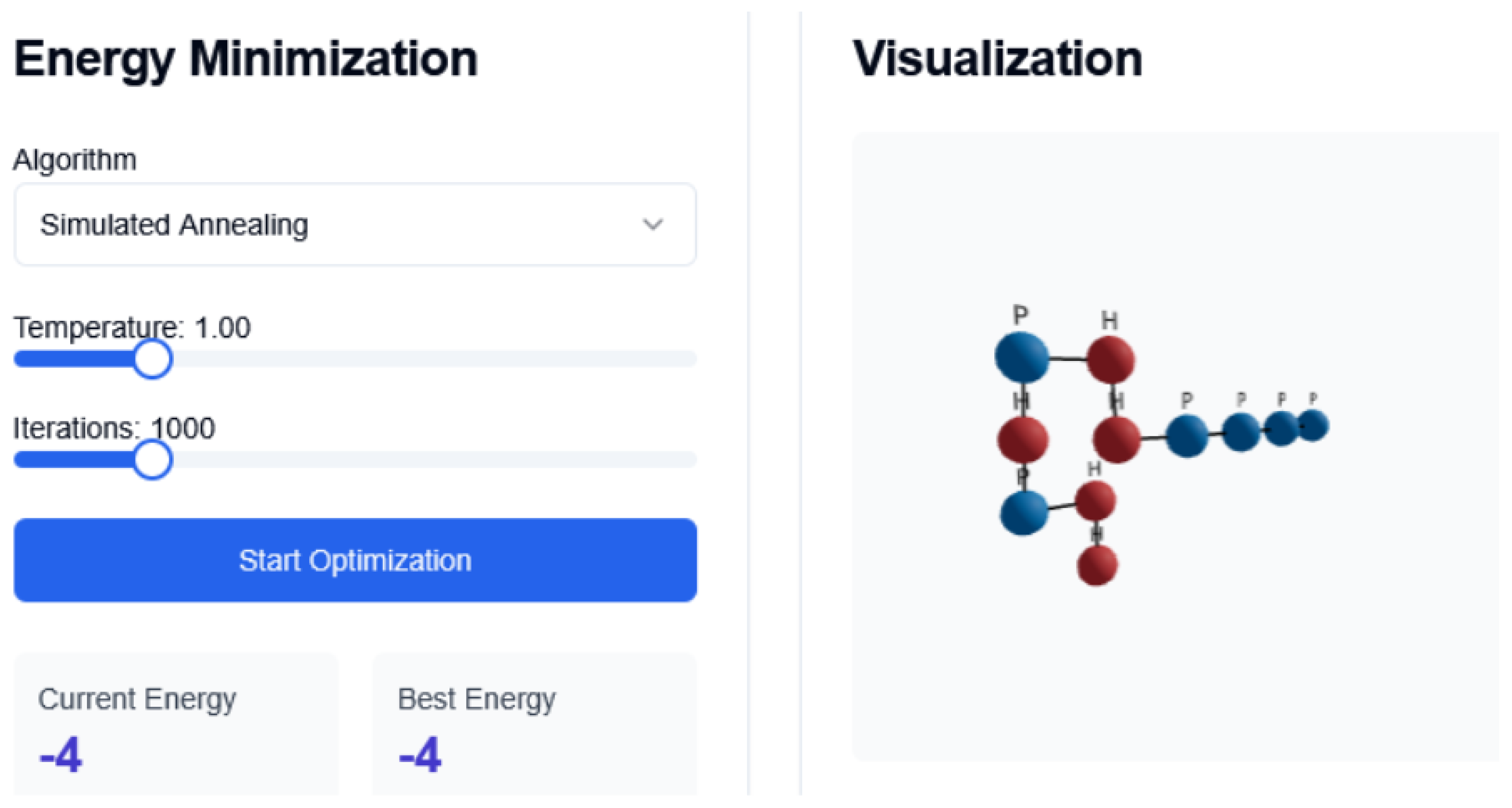
The Simulated Annealing (SA) algorithm also ran for 1000 iterations, starting from an initial temperature , which was gradually decreased using an exponential cooling schedule:
where is the temperature at iteration k; is the initial temperature; is the cooling rate, and k is the iteration index.
Figure 4.
SA Energy evolution
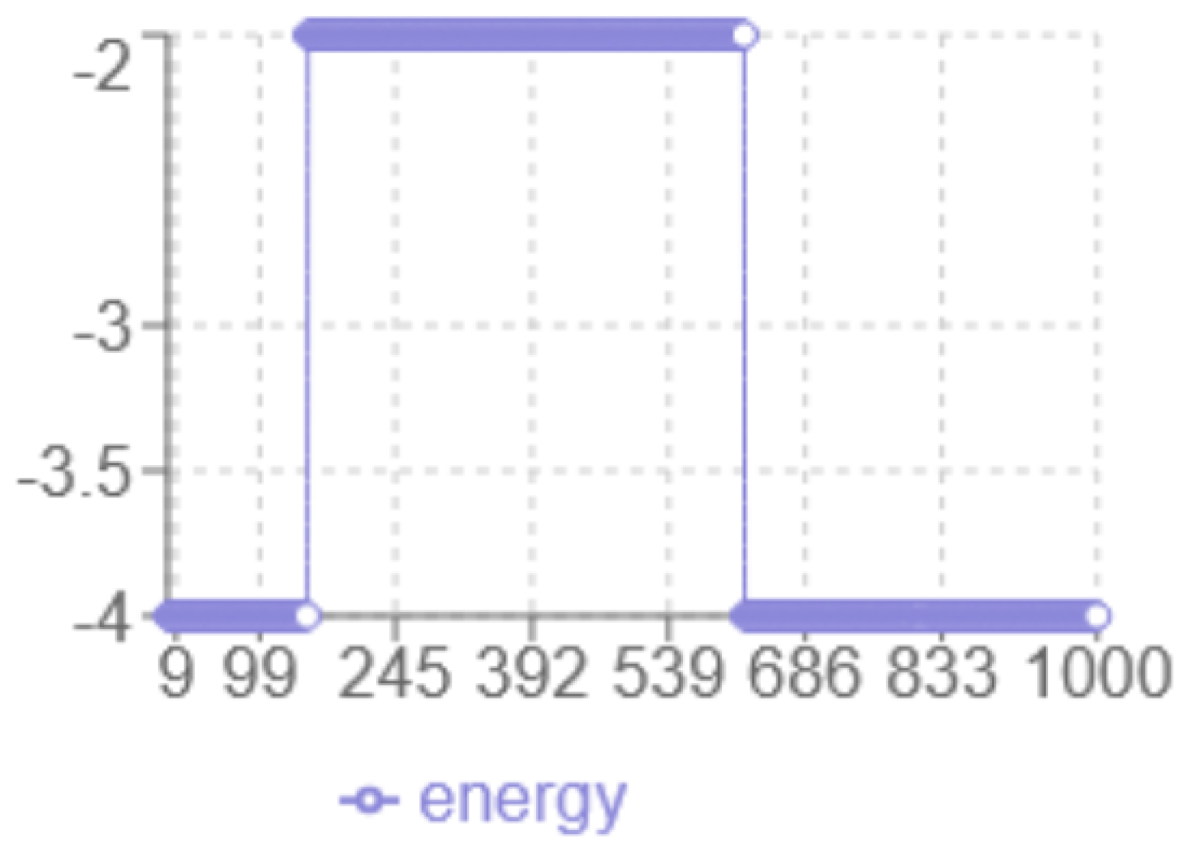
According to the energy analysis in Figure 4, the following observations were made: the x-axis corresponds to the iteration number, while the y-axis represents the energy level multiplied by two. The minimum energy achieved is , which is lower than the result obtained with the Monte Carlo method. The dynamic behaviour shows a smooth transition from -2 to -3.5 without abrupt jumps, and a noticeable plateau around -2, indicating prolonged exploration in that region. The final structure have increased linearity with fewer compact hydrophobic interactions, suggesting potential risks in a local optimum.
4.3. ACGA Algorithm
The proposed ACGA is a population-based method that evolves a set of protein conformations using selection, crossover, and mutation operations. The fitness function incorporates both energy minimisation and structural compactness metrics. ACGA involves the following steps:
- Population Initialization: Firstly, a population of potential solutions is created. Each solution, referred to as a chromosome, is randomly generated, and it has an associated objective function called fitness.
- Exploration Stage: The mutation and crossover operators are applied to a certain percentage of the chromosomes in the population, which are chosen randomly. These operators ensure the dispersion of the population in the space of possible solutions, promoting exploration of the solution space.
- Through the selection operation, from a percentage of the individuals of the population, those with the best fitness are selected. In this way, a new population is created, usually statistically better, and this represents the next generation.
- Exploitation Stage: Through the selection operation, a certain percentage of individuals with the best fitness are chosen from the population. This process creates a new population, which is usually statistically better and represents the next generation of potential solutions. The selection operation helps exploit the combinatorial space by favoring the fitter individuals for reproduction.
Steps 2) and 3) are iterated for a number of generations, allowing the population to evolve and improve over time. The mutation and crossover operators contribute to the exploration stage, while the selection operator contributes to the exploitation stage of the genetic algorithm.
Chromosomes encoding. We consider that the conformation of the modeled proteins can be encoded using either relative or absolute directions. We have chosen to use both in our approach to exploit the advantages of both encodings. The benefits of using relative encoding are as follows: a) smaller combinatorial space compared to absolute encoding (relative – ; absolute – ); b) implicit avoidance of returning the current AA to the previous AA position in the walk, during the creation of the initial population. c) Mutation and crossover operators do not require modifications of letters that specify the next positions. On the other hand, absolute coding allows easy conversion into Cartesian coordinates.
Therefore, we have employed both the absolute and relative encodings, resulting in the following corresponding representations (strings):
- string
- string – absolute 2D square
- string – relative 2D square
- string –absolute 3D cubic
- string – relative 3D cubic
string is a string. We will generically call string, string, string and string as strings.
For computational efficiency reasons, the exploration is performed using the relative encoding, which reduces the time complexity from to . However, the corresponding absolute encoding is also stored to enable easy and fast computation of the Cartesian coordinates.
The size of the string is equal to n, and the size of the strings is equal to , with each letter representing the relative successive direction in the conformation, where n is number of AAs of the sequence.
Generation of the initial population. The string represents the input data, and the string is the output of the ACGA algorithm. The primary structure of the protein is represented by the string ( string) of n letters corresponding to the n AAs of a sequence.
Below are the steps for building a conformation (chromosome) using string representation in the population initialization stage:
- Set i = 1. Initialize SRL[i] = ’S’.
- i = i + 1. if continue with the next step. Otherwise, the conformation is completely generated in the string.
- Choose a random direction ’d’ from the {S,R,L}.
For the 3D case, a similar construction is used based on the string.
Then, the string is converted to the string. The first letter, which is S, is always converted to the R letter. This fact reduces the 4-exponential combinatorial space by four times. After that, the string is converted to an array of Cartesian coordinates. Based on these Cartesian coordinates, the number of collisions, the number of contacts, and the fitness are computed.
The math formulas used for finding an H-H contact in the 2D square and 3D cubic lattices are as follows.
- For the 2D square lattice:
- If ,
where , are the Cartesian coordinates of the i-th AA, and , are the Cartesian coordinates of the j-th AA, then there is a contact between the two AAs at positions i and j, .
- For the 3D cubic lattice:
- If ,
where , , are the Cartesian coordinates of the i-th AA, and , , are the Cartesian coordinates of the j-th AA, then there is a contact between the two AAs at positions i and j, .
For finding a collision (two AAs in the same place), we use the following equations, where the terms have the same understanding as above:
- For 2D square lattice, if : ;
- For 3D cubic lattice, if :
If these equations are satisfied, it indicates that there is a collision between the AAs at positions i and j in the conformation.
Figure 5 presents two conformations: on the left side, there is a SAW conformation, and on the right side, there is a conformation that has one collision (non-SAW conformation).
Fitness Evaluation Strategy. The fitness function evaluates how close a given chromosome is to the optimum solution. It determines how fit a chromosome is. We have used a fitness function inspired by the code of Alican Toprak 1.
where c is the conformation, is the number of contacts, and the is the number of collisions of the conformation. This is computed by checking the topological neighborhood of all AAs on the lattice, according to the number of contacts (Equation 2) and the number of collisions (). There are two exceptions: if then the formula becomes and if then is replaced with 2. Thus, the fitness increases with the number of contacts and is strongly penalized by the number of collisions.
Figure 6.
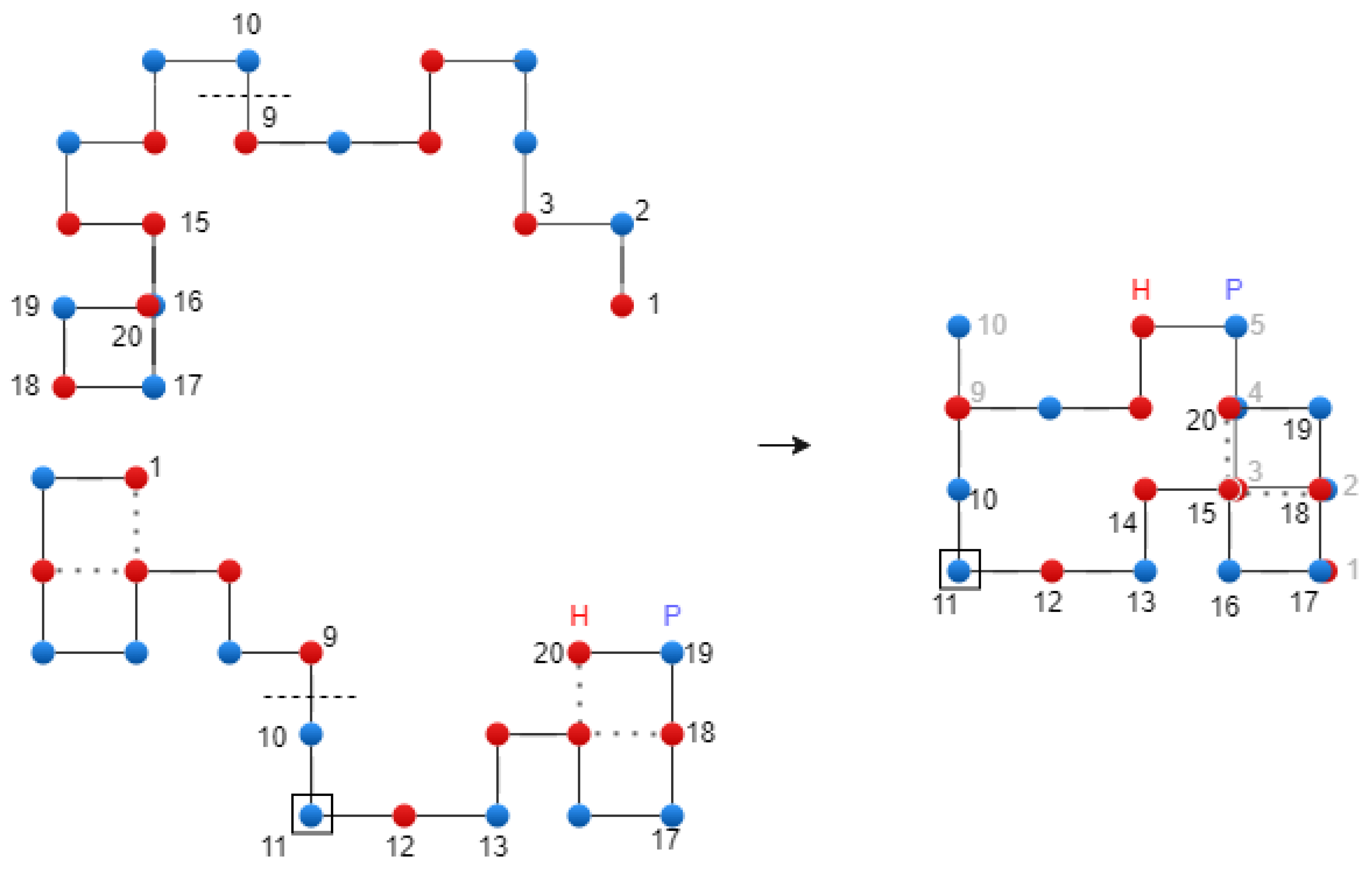
Translational crossover on the 2D Lattice – exemplification.
Adapted tournament selection. We proposed an adapted variant of tournament selection, which increases the probability of individuals with low energy values entering the next generation, while implicitly conserving the best individual. Specifically, the selection is applied to the previous population by choosing pairs of chromosomes at random, and after comparing them, the best one is copied into the position of the worst one. This way, the best chromosome is preserved through the generations.
Rotational crossover. In addition to the rotational crossover used in our previous work [43], we apply the translational crossover. For both types of crossover operators, the best chromosome () from the current population is protected. The crossover operation is performed using the following formula:
where is the best chromosome from the current population, and and are parent chromosomes. The reason for introducing , as parameter into the crossover operator is to protect this chromosome. Figure 6 shows the translational crossover.
Translational mutation. We employ translational, rotational, and diagonal mutations. Given a chromosome , where for 2D (or for 3D), it is mutated to a new chromosome, C’. To achieve this, a position g (1 ≤ g ≤ n), known as the mutation point, is randomly chosen for each conformation. The letter at position g is then replaced by one letter sampled uniformly from the set of possible directions.
For the rotational mutation, the modification is applied to the string, and the next letter after the g point remains unchanged. Then, the string is converted to the string. This modification produces a rotation of the second part of the chain by 90°, 180°, or 270°, respectively. In the case of translational mutation, the modification is applied to the string, and the next letter after the g point remains unchanged. Figure 7 shows the two types of mutation. A diagonal move is executed on the two letters of the string that form a corner. Finally, the mutation operation is performed using the following formula:
where is the best chromosome from the current population and t represents the iteration number (time). The reason for introducing , as parameter into the mutation operator is to protect it.
The algorithm. The steps of the algorithm establish the generation number. For every generation, the next operations are executed: a) rotational crossover, b) translational crossover, c) translational mutation, d) rotational mutation, e) diagonal mutation, and f) tournament selection. After iterating all generations, the algorithm returns the best conformation obtained.
Pseudocode of the ACGA algorithm skeleton is given in Algorithm 1.
| Algorithm 1 All Conformations Genetic Algorithm (ACGA) |
|
Figure 7.
Rotational and translational mutation on the 2D Lattice – exemplification.

5. Results Analysis
The algorithm has been implemented in the C++ programming language, and tests were conducted on a PC with a Intel(R) Core i7, 2.8 GHz, processor with 4 physical CPU and 4 logical CPU, and 8 GB of RAM running Windows 10. Two implementation variants were developed: one using an OOP style for better software qualities (readability, maintainability, usability) but with slightly poorer execution time performance, and another using the standard C style, which is approximately 40 times faster, mainly due to a more optimized implementation of the selection operation. The results presented in this report are based on the second implementation variant.
To evaluate the efficiency of the algorithm, experiments were conducted on nine popular benchmark sequences with varying lengths ranging from 20 AAs to 85 AAs (see Table 1). The first eight sequences were taken from Unger1993 [9], and the ninth sequence was taken from Huang2010 [16] The table contains information about the sequence ID, the protein length, and the string.
The population size and the number of generations were chosen to allow a wide range of possible conformations to be evaluated. For the selection, mutation, and crossover operators, we tested multiple configurations and adopted the ones that produced the best results after parameter tuning. For the algorithm parameters, we considered various combinations of the following parameters to explore the solution space:
1). Population size: 10, 50, 100, 300, 500, 1000, 2000, 5000, 10000, 20000, 50000;
2). Number of generations: 50, 100, 200, 300;
3). Translational mutation percent: 0.3;
4). Rotational crossover percent: 0.4;
5). Adapted tournament selection percent: 0.35.
For each combination, we repeated the execution 20 times and computed the average energy obtained. We have established 20 considering the aspect to have enough data to have enough data to be able to make simple (like data normality assumption verification) or even advanced statistical analyses (combined analyses where different assumptions must be met).
Table 2 shows the best results obtained for the nine benchmark sequences, which are highly influenced by the population size. The empty value represents that we have no data in the literature for it.
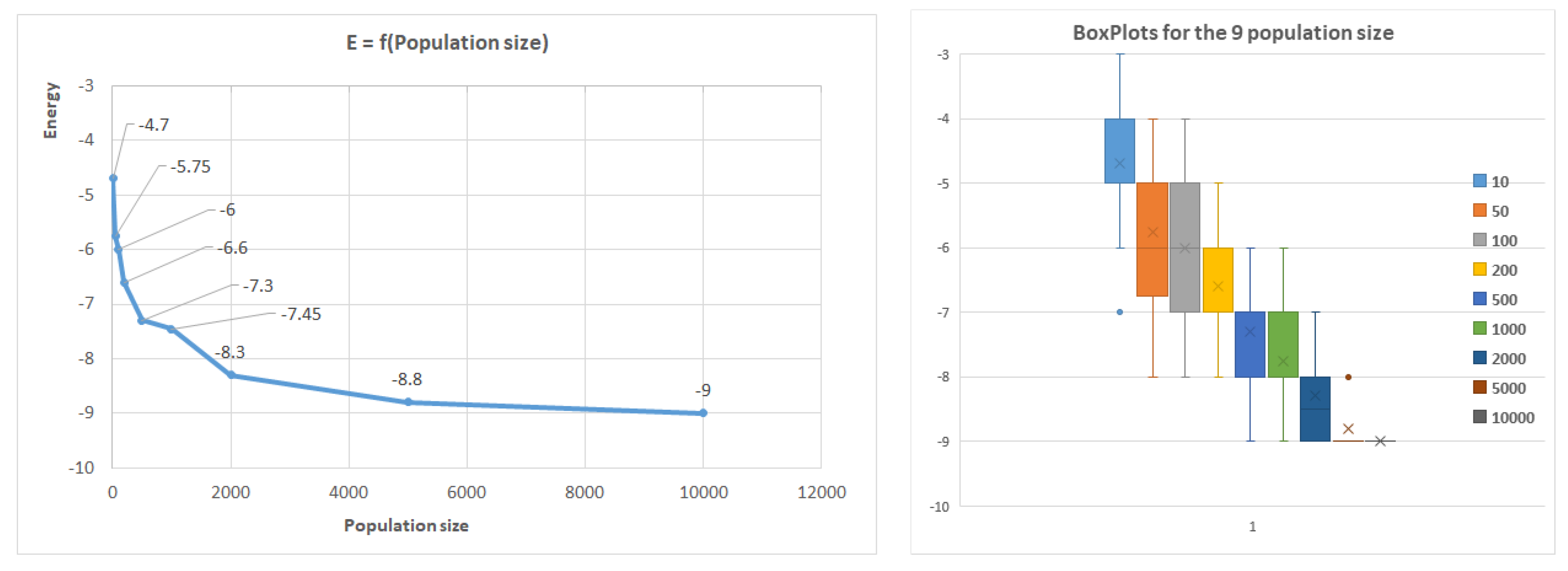
Figure 8 further illustrates how the population size affects the results, with the first benchmark sequence of length 20 used as an example. Similar trends were observed for other sequences, where shorter sequences (less than 50 AAs) reached optimal conformations rapidly by increasing the population size, while longer sequences did not reach the optimum.
The algorithm indicates good convergence, as the optimum conformation is typically achieved within 100 generations for small conformations. However, for larger conformations, significant improvements were not observed after 100 generations. The algorithm’s robustness was confirmed by repeating executions with the same parameters 20 times, resulting in a relatively low standard deviation. The box plot in Figure 8 presents the quartile median calculus.
Table 3 and Table 4 show the best conformations obtained by ACGA for the 2D square and 3D cubic lattices, respectively. In conclusion, even for long proteins, the ACGA approach offers a reasonable possibility of finding solutions very close to the optimal ones.

Table 2.
Best energy for 2D and 3D square lattice for the 9 considered benchmarks.
| ID Seq | Length | Optimal 2D | ACGA 2D | Optimal 3D | ACGA 3D |
|---|---|---|---|---|---|
| 1 | 20 | -9 | -9 | -11 | -11 |
| 2 | 24 | -9 | -9 | -13 | -13 |
| 3 | 25 | -8 | -8 | -9 | -9 |
| 4 | 36 | -14 | -14 | -18 | -18 |
| 5 | 48 | -23 | -22 | -31 | -31 |
| 6 | 50 | -21 | -21 | -34 | -31 |
| 7 | 60 | -36 | -35 | -55 | -49 |
| 8 | 64 | -42 | -38 | -59 | -49 |
| 9 | 85 | -53 | -48 | - | -73 |
Table 3.
2D conformations obtained by ACGA for the benchmark sequences.
| ID Seq | Optimal conformations on 2D square HP model |
|---|---|
| 1 | ULLDRDLDLDRRURDRUUL |
| 2 | LULDLDRDRURRRDRURULULDL |
| 3 | RULURUUURDDRURDDLDRDLLUU |
| 4 | LDLDRDLDDLLURULLURRUULDLUULDDDLDRDD |
| 5 | RURDRURDRRRDLDLULDLULDLULDLDRRRDLDRRRRURULLLDR |
| 6 | RDLLUURURDRURDRDLLDDLLDLLLLLLUULURRURDDLDRRURUULD |
| 7 | URDDDRUURDDDLDRRUUUUULLURRURRRRDLDLULDDRRRURDDLLLLDRRDLLDRR |
| 8 | RDLLULDLULDLUURURDRURDRRRDRDLDRDLDRDLDLULDLULDDLUUURRRRULLLURRR |
| 9 | RRRRULLLURULLDDLULDLLDLUUURDRURRURRUUULDDLLDLULDLLDLUURRURRRRULLLLLLURURDRURDRURRDL |
Table 4.
3D conformations obtained by ACGA for the benchmark sequences.
| ID Seq | Optimal conformations on 3D square HP model |
|---|---|
| 1 | DLLURUFDLDRRUUURDBL |
| 2 | RRULUBDRDLDLUBUFULDLFRR |
| 3 | RBRULUURBLDDRDLLUULLFRRD |
| 4 | FLLLDRFLLLURURDRFDLULURRURDBLBULDLL |
| 5 | DRDRURRULURULLLDDRUFRDLDRFFLLURBRRULLULDLBRDFDB |
| 6 | RDLLULFDRURDRURULLUBDLLUFRDLFDRUURDRDLDLFRRUULLDR |
| 7 | RDLFRDLDRRURDDBLURULLLDRDLLUUUBRRDLDRRRULBDRDLLUUULDDDFRDLD |
| 8 | BRRULLFRDRURDDLLFURRULLULDLDRDDFURDRURULLLURRRULLFFDRDLDRBUULDD |
| 9 | FFLDLBRRDRRUULDBURDDDRFLFULLURURDRUBDRFFLULDLDLLURULURRDFRDLDLUULDDLFRULURRURDDRDLLU |
Figure 8.
Average energy related to population size in the case of the first benchmark.
The Web-Based Tool for 3D Protein Folding supports five molecular visualisation modes:
- 2D Grid View – Classic square lattice with H and P residues colour-coded.
- 3D Grid View – Cubic lattice with interactive 3D navigation.
- Ribbon View – Stylised representation highlighting the protein backbone.
- Space-filling View – Van der Waals surface model showing spatial occupation.
- Surface View – Solvent-accessible surface representation.
Comparison 1. The comparative analysis of the implemented algorithms gave the following observation: The following conclusion was drawn from the comparative study of the implemented algorithms:
- MC achieved the best energy result () and demonstrated dynamic search behaviour with strong exploratory capability. However, due to its fixed temperature, it is prone to high fluctuations and occasional instability.
- SA displayed smoother convergence, better stability, and was more resilient to local optima thanks to its cooling schedule. Nonetheless, it resulted in a slightly higher final energy (), indicating slower convergence in practice.
- GA was effective at exploring diverse conformations and maintaining population diversity. Its performance depends strongly on the balance between exploration and exploitation parameters, such as mutation rate and selection pressure.
Comparison 2. In comparison with the CPSP-tools suite [44,45], developed at the University of Freiburg, HP Protein Visualizer offers a more integrated and interactive approach. While both tools enable minimum energy computation and H-H contact identification in HP lattice models, the Visualizer extends functionality by providing detailed energy distribution plots, contact maps, geometric descriptors, and solvent-accessibility metrics. Moreover, it allows for side-by-side structure comparison. In terms of integration and export capabilities, HPview is limited to basic PDB output with minimal compatibility, whereas HP Protein Visualizer supports export in multiple formats, including PDB, CSV, JSON, and SVG.
6. Discussion
MC proved the advantage of including fast convergence to good solutions, simplicity of implementation, and high efficiency in small search spaces. However, the limitations include a risk of restriction in local optima due to the fixed temperature, and large fluctuations that may lead to inconsistent solutions.
SA proved a better avoidance of local optima due to its controlled cooling mechanism, stable convergence without extreme oscillations, and robust performance in complex search spaces. Its disadvantages include slower convergence (requiring more iterations) and, in this case, a suboptimal final energy compared to MC (-3.5 compared to -4).
The ACGA algorithm was efficiently optimized from a computational point of view, enabling the use of large populations to maintain the diversity of individuals in the context of limited computing resources. Experiments have been conducted for several benchmark HP sequences, and the comparative analysis showed that the proposed genetic algorithms offer valuable advantages for PSP on the HP model, providing optimal solutions in most cases, i.e., from a maximum of 20 trials, we give the standard deviation.
In comparison to all these previous results, our approach addresses both 2D square and 3D cubic cases, and we achieved optimum conformations for sequences of length less than or equal to 50. Concerning the 2D square and 3D cubic models, our results are similar for larger sequences.
Unlike HP Protein Visualizer, which prioritises exploratory use and algorithmic approaches through simplified lattice models AlphaFold and RoseTTAFold aim for highly accurate real-world predictions. While they require substantial computational resources, HP-based tools can be executed in a web browser and are more accessible for didactic and exploratory use.
7. Conclusion
The HP model is an ab initio paradigm to model and understand protein folding and is one of the most extensively studied physical models for protein structure prediction from sequences. While the HP model appears very simple, solving it is proven NP-hard. Based on this fact, it is a very good benchmark problem for GA.
We have introduced a novel hybrid Genetic Algorithm that also offers interpretability for PSP that goes beyond considering only the SAW conformations. Instead, our approach allows any conformations in the populations at all stages. This increased flexibility improves the likelihood of obtaining good conformations, even starting from non-SAW ones, as the energy associated with these conformations shows chaotic behavior.
Our primary focus has been on computational efficiency, as it enables reasonable computation times even for large populations. Working with large populations is crucial to achieving the necessary diversity for convergence. The results obtained on a popular benchmark dataset are highly promising, with the optimal solution being achieved in most cases, and for others, the distance from the optimal solution is minimal.
To further improve the algorithm, we plan to explore parallel computation, which can significantly enhance computational performance, allowing the use of even larger populations. Larger populations further increase the chances of reaching optimal solutions for all cases. Parallelization will be a key focus of our future work. Additionally, we intend to apply the parallel AGCA to real proteins and compare its results with the native conformations from the Protein Data Bank (PDB) [27] and those obtained using the AlphaFold algorithm. This comparison will provide valuable insights into the performance of our algorithm on real biological proteins.
Author Contributions
Conceptualization, I.S.; methodology, I.S.; software, I.S., C.-D.M; validation, I.S., C.-D.M.; formal analysis, I.S., C.-D.M. and I.-L.B.; investigation, I.S., C.-D.M., I.-L.B.; resources, I.S., C.-D.M.; data curation, I.S.; writing—original draft preparation, I.S. and C.-D.M.; writing—review and editing, C.-D.M and I.-L.B.; visualization, I.S., C.-D.M., I.-L.B.; supervision, I.-L.B.; project administration, I.S. and C.-D.M.; funding acquisition, C.-D.M. All authors have read and agreed to the published version of the manuscript.
Funding
This research received no external funding.
Institutional Review Board Statement
Not applicable.
Informed Consent Statement
Not applicable.
Data Availability Statement
Acknowledgments
This research received financial support from ’1 Decembrie 1918’ University of Alba Iulia, Romania, through Order no. 3259 of 13th February 2025. The authors thank the Research Group on Artificial Intelligence and Data Science for Healthcare Innovation (REFLECTION) and the Research Center on Artificial Intelligence, Data Science, and Smart Engineering (ARTEMIS), of the George Emil Palade University of Medicine, Pharmacy, Science and Technology of Targu Mureş, Romania, for support of research infrastructure. The CA22137 COST Action, the Randomized Optimization Algorithms Research Network (ROAR-NET), with concerns in identifying benchmarking issues. The authors thank Eng. Simona Ispas, is responsible for the graphic design.
Conflicts of Interest
The authors declare no conflicts of interest.
References
- Baynes, J.W.; Dominiczak, M.H. Medical Biochemistry FIFTH EDITION; Elsevier, 2019. fifth edition.
- Felix-Saul, J.C.; García-Valdez, M.; Merelo Guervós, J.J.; Castillo, O. Extending Genetic Algorithms with Biological Life-Cycle Dynamics. Biomimetics 2024, 9. [CrossRef]
- Rashid, M.; Newton, M.A.H.; Hoque, M.; Sattar, A. Mixing Energy Models in Genetic Algorithms for On-Lattice Protein Structure Prediction. BioMed research international 2013, 2013, 924137. [CrossRef]
- Rashid, M.A.; Iqbal, S.; Khatib, F.; Hoque, M.T.; Sattar, A. Guided macro-mutation in a graded energy based genetic algorithm for protein structure prediction. Computational Biology and Chemistry 2016, 61, 162–177. [CrossRef]
- Hardy, J.; Selkoe, D.J. Amyloid hypothesis of Alzheimer’s disease: progress and problems on the road to therapeutics. Science 2002, 297, 353–356.
- Leaver-Fay, A.; .; et al. Rosetta3: an object-oriented software suite for the simulation and design of macromolecules. Methods in enzymology 2011, 487, 545–574.
- Abraham, M.J.; et al. GROMACS: High performance molecular simulations through multi-level parallelism from laptops to supercomputers. SoftwareX 2015, 1, 19–25.
- Anfinsen, C.B. Principles that govern the folding of protein chains. Science 1973, 181, 223–230.
- Unger, R.; Moult, J. Genetic algorithms for protein folding simulations. Journal of molecular biology 1993, 231 1, 75–81.
- Custódio, F.; Barbosa, H.; Dardenne, L. Investigation of the three-dimensional lattice HP protein folding model using a genetic algorithm. Genetics and Molecular Biology - GENET MOL BIOL 2004, 27. [CrossRef]
- Jiang, T.; Cui, Q.; Shi, G.; Ma, S. Protein folding simulations of the hydrophobic–hydrophilic model by combining tabu search with genetic algorithms. The Journal of Chemical Physics 2003, 119, 4592–4596. [CrossRef]
- Cox, G.; Mortimer-Jones, T.; Taylor, R.; Johnston, R. Development and optimisation of a novel genetic algorithm for studying model protein folding. Theoretical Chemistry Accounts 2004, 112, 163–178. [CrossRef]
- Cox, G.; Johnston, R. Analyzing energy landscapes for folding model proteins. The Journal of chemical physics 2006, 124, 204714. [CrossRef]
- Liang, F.; Wong, W.H. Evolutionary Monte Carlo for protein folding simulations. The Journal of Chemical Physics 2001, 115, 3374–3380. [CrossRef]
- Zhou, C.; et al. Enhanced hybrid search algorithm for protein structure prediction using the 3D-HP lattice model. Journal of Molecular Modeling 2013, 19, 3883–3891. [CrossRef]
- Huang, C.; Yang, X.; He, Z. Protein folding simulations of 2D HP model by the genetic algorithm based on optimal secondary structures. Computational biology and chemistry 2010, 34, 137–42. [CrossRef]
- Benitez, C.; Parpinelli, R.; Lopes, H. Parallelism, hybridism and coevolution in a multi-level ABC-GA approach for the protein structure prediction problem. Concurrency and Computation: Practice and Experience 2011, 24, 635 – 646. [CrossRef]
- Rashid, M.; Newton, M.A.H.; Hoque, M.; Sattar, A. A local search embedded genetic algorithm for simplified protein structure prediction. In Proceedings of the 2013 IEEE Congress on Evolutionary Computation, CEC 2013, 06 2013. [CrossRef]
- Rashid, M.A.; Newton, M.H.; Hoque, M.T.; Sattar, A. Collaborative Parallel Local Search for Simplified Protein Structure Prediction. In Proceedings of the 2013 12th IEEE International Conference on Trust, Security and Privacy in Computing and Communications, 07 2013, pp. 966–973. [CrossRef]
- Dill, K.A. Theory for the folding and stability of globular proteins. Biochemistry 1985, 24, 1501.
- Lau, K.F.; Dill, K.A. A lattice statistical mechanics model of the conformational and sequence spaces of proteins. Macromolecules 1989, 22, 3986–3997. [CrossRef]
- Boumedine, N.; Bouroubi, S. A new hybrid genetic algorithm for protein structure prediction on the 2D triangular lattice. TURKISH JOURNAL OF ELECTRICAL ENGINEERING AND COMPUTER SCIENCES 2021, 29, 499–513. [CrossRef]
- Mazidi, A.; Roshanfar, F. PSPGA: A New Method for Protein Structure Prediction based on Genetic Algorithm. Journal of Applied Dynamic Systems and Control 2020, 3, 9–16.
- Rezaei, M.; Kheyrandish, M.; Mosleh, M. A novel algorithm based on a modified PSO to predict 3D structure for proteins in HP model using Transfer Learning. Expert Systems with Applications 2024, 235, 121233. [CrossRef]
- S., G.; E.R., V. Protein Secondary Structure Prediction Using Cascaded Feature Learning Model. Applied Soft Computing 2023, 140, 110242. [CrossRef]
- Berger, B.; Leighton, T. Protein Folding in the Hydrophobic-Hydrophilic (HP) Model is NP-Complete. Journal of Computational Biology 1998, 5, 27–40. [CrossRef]
- Burley, S.K.; et al. RCSB Protein Data Bank (RCSB.org): delivery of experimentally-determined PDB structures alongside one million computed structure models of proteins from artificial intelligence/machine learning. Nucleic Acids Research 2023, 51, D488–D508. [CrossRef]
- Chira, C.; Horvath, D.; Dumitrescu, D. Hill-Climbing search and diversification within an evolutionary approach to protein structure prediction. BioData mining 2011, 4, 23. [CrossRef]
- Rotar, C. An Evolutionary Technique for Multicriterial Optimization Based on Endocrine Paradigm. 06 2004, Vol. 3103, pp. 414–415. [CrossRef]
- Bahi, J.M.; Cote, N.; Guyeux, C. Chaos of Protein Folding. Neural Networks (IJCNN) 2011, pp. 1948–1954.
- Bahi, J.M.; Côté, N.; Guyeux, C.; Salomon, M. Protein Folding in the 2D Hydrophobic–Hydrophilic (HP) Square Lattice Model is Chaotic. Cognitive Computation 2011, 4, 98–114.
- Jumper, J.; Evans, R.; Pritzel, A.; Green, T.; Figurnov, M.; Ronneberger, O.; Tunyasuvunakool, K.; Bates, R.; Zidek, A.; Potapenko, A.; et al. Highly accurate protein structure prediction with AlphaFold. Nature 2021, 596, 583–589.
- Callaway, E. What’s next for AlphaFold and the AI protein-folding revolution. Nature 2022, 604, 234–238.
- Krishna, R.; et al. Generalized biomolecular modeling and design with RoseTTAFold All-Atom. Science 2024, 384, eadl2528. [CrossRef]
- Baek, M.; DiMaio, F.; Anishchenko, I.; Dauparas, J.; Ovchinnikov, S.; Lee, G.R.; Wang, J.; Cong, Q.; Kinch, L.N.; Schaeffer, R.D.; et al. Accurate prediction of protein structures and interactions using a three-track neural network. Science 2021, 373, 871–876.
- Cruz-Fernández, M.; et al. Model Parametrization-Based Genetic Algorithms Using Velocity Signal and Steady State of the Dynamic Response of a Motor. Biomimetics 2025, 10. [CrossRef]
- Crescenzi, P.; Goldman, D.; Papadimitriou, C.; Piccolboni, A.; Yannakakis, M. On the Complexity of Protein Folding. Journal of Computational Biology 1998, 5, 423–465. [CrossRef]
- Zhang Hongjin, W.H. Enhanced genetic algorithm for indoor low-illumination stereo matching energy function optimization. Alexandria Engineering Journal 2025, 121, 1–17. [CrossRef]
- Cristea, D. Hybrid Combinatorial Problems Used for Multimodal Optimisation. In Proceedings of the 2024 IEEE 24th International Conference on Bioinformatics and Bioengineering (BIBE), 2024, pp. 1–8.
- Sauer, R.T. Protein folding from a combinatorial perspective. Folding and Design 1996, 1, R27 – R30. [CrossRef]
- Metropolis, N.; Rosenbluth, A.W.; Rosenbluth, M.N.; Teller, A.H.; Teller, E. Equation of state calculations by fast computing machines. The journal of chemical physics 1953, 21, 1087–1092.
- Kirkpatrick, S.; Gelatt, C.; Vecchi, M. Optimization by simulated annealing. Science 1983, 220, 671–680.
- Sima, I.; Parv, B. Protein Folding Simulation Using Combinatorial Whale Optimization Algorithm. In Proceedings of the 2019 21st International Symposium on Symbolic and Numeric Algorithms for Scientific Computing (SYNASC), 2019, pp. 159–166.
- Mann, M.; Backofen, R.; Will, S. Faster exact protein structure prediction with the CPSP approach. Constraints 2005, 10, 5–30.
- Milde, F.; Giegerich, R.; Will, S. CPSP-tools–Exact and complete algorithms for high-throughput 3D lattice protein studies. In Proceedings of the Bioinformatics Research and Applications. Springer, 2010, pp. 21–32.
Figure 5.
Conformations on 2D Lattice.
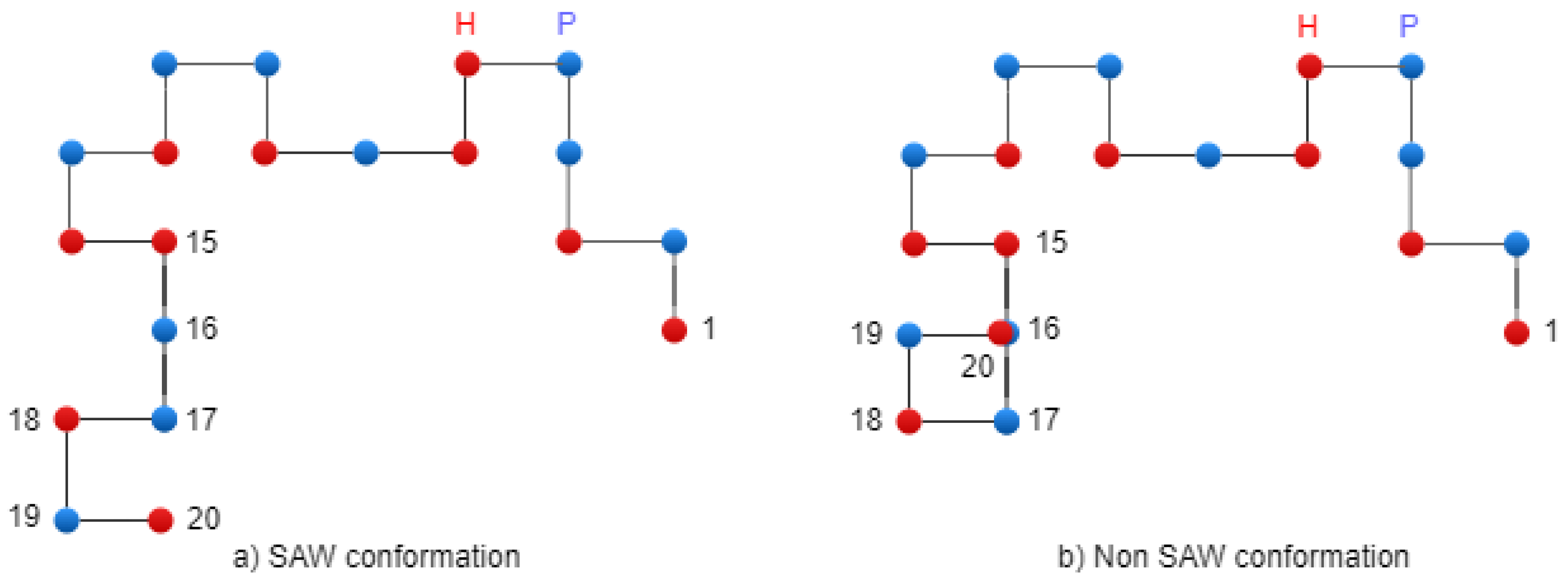
Table 1.
Benchmark data set
| ID | No of | Sequence |
|---|---|---|
| Seq | AA | |
| 1 | 20 | HPHP PHHP HPPH PHHP PHPH |
| 2 | 24 | HHPP HPPH PPHP PHPP HPPH PPHH |
| 3 | 25 | PPHP PHHP PPPH HPPP PHHP PPPH H |
| 4 | 36 | PPPH HPPH HPPP PPHH HHHH HPPH HPPP PHHP PHPP |
| 5 | 48 | PPHP PHHP PHHP PPPP HHHH HHHH HHPP PPPP HHPP HHPP HPPH HHHH |
| 6 | 50 | HHPH PHPH PHHH HPHP PPHP PPHP PPPH PPPH PPPH PHHH HPHP HPHP HH |
| 7 | 60 | PPHH HPHH HHHH HHPP PHHH HHHH HHHP HPPP HHHH HHHH HHHH PPPP HHHH HHPH HPHP |
| 8 | 64 | HHHH HHHH HHHH PHPH PPHH PPHH PPHP PHHP PHHP PHPP HHPP HHPP HPHP HHHH HHHH HHHH |
| 9 | 85 | HHHH PPPP HHHH HHHH HHHH PPPP PPHH HHHH HHHH HHPP PHHH HHHH HHHH HPPP HHHH |
| HHHH HHHH PPPH PPHH PPHH PPHPH |
Disclaimer/Publisher’s Note: The statements, opinions and data contained in all publications are solely those of the individual author(s) and contributor(s) and not of MDPI and/or the editor(s). MDPI and/or the editor(s) disclaim responsibility for any injury to people or property resulting from any ideas, methods, instructions or products referred to in the content. |
© 2025 by the authors. Licensee MDPI, Basel, Switzerland. This article is an open access article distributed under the terms and conditions of the Creative Commons Attribution (CC BY) license (http://creativecommons.org/licenses/by/4.0/).
Copyright: This open access article is published under a Creative Commons CC BY 4.0 license, which permit the free download, distribution, and reuse, provided that the author and preprint are cited in any reuse.


