
Submitted:
28 June 2025
Posted:
01 July 2025
You are already at the latest version
Abstract
We give for the first time explicit formulas for the coefficients needed for the 4th order Edgeworth expansions of a multivariate standard estimate. We call these the Edgeworth coefficients. They are Bell polynomials in the cumulant coefficients. Standard estimates include most estimates of interest, including smooth functions of sample means and other empirical estimates. We also give applications to ellipsoidal and hyperrectangular sets.
Keywords:
Edgeworth expansions
; standard estimates
; multivariate Edgeworth coefficients
; ellipsoidal and hyperrectangular sets
1. Introduction and Summary
Suppose that is a standard estimate, as defined in §2, of an unknown parameter of a statistical model, based on a sample of size n. For example may be a smooth function of a sample mean, or a smooth functional of an empirical distribution. A smooth function of a standard estimate is also a standard estimate: see Withers (2024). §2 summarises the multivariate Edgeworth expansions of Withers and Nadarajah (2010) for the distribution and density of in powers of about the multivariate normal in terms of the Edgeworth coefficients, the -coefficients of (11). For , these are needed for the st term of the multivariate Edgeworth expansions. They are Bell polynomials in the cumulant coefficients of (5). They are given for by (12) and for by (12)–(14) in terms of the symmetrizing operator , and explicitly in Appendix A. §3 derives expansions on ellipsoidal and hyperrectangular sets.
When , §4 simplifies these Edgeworth coefficients using dual notation. Examples include the distribution and density of a sample mean, and of bivariate entangled gamma random variables.
§5 and §6 give conclusions and discussion, and suggests some future directions. Appendix B gives explicitly the bivariate Hermite polynomials needed for bivariate Edgeworth expansions to .
Univariate estimates. Suppose that is a standard estimate of with respect to n, (typically the sample size). That is, is non-lattice,
as , and its rth cumulant can be expanded as
where the cumulant coefficients may depend on n but are bounded as , and is bounded away from 0. Here and below ≈ indicates an asymptotic expansion that need not converge. So (1) holds in the sense that
where means that is bounded in n. Withers (1984) replaced the artifical assumptions of Cornish and Fisher (1937) and Fisher and Cornish (1960) by (1), and gave the distribution, density and quantiles of
as asymptotic expansions in powers of :
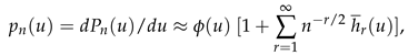
 where is the probability that A is true,
is a unit normal random variable with even moments , and are polynomials in u and also in the standardized cumulant coefficients . For example
where is the kth Hermite polynomial. By Withers (2000), for ,
(A1) gives for . Since is even/odd for r odd/even,
From (4), it follows that
For a discussion of when to truncate (2)–(4), see Withers and Nadarajah (2012a).
where is the probability that A is true,
is a unit normal random variable with even moments , and are polynomials in u and also in the standardized cumulant coefficients . For example
where is the kth Hermite polynomial. By Withers (2000), for ,
(A1) gives for . Since is even/odd for r odd/even,
From (4), it follows that
For a discussion of when to truncate (2)–(4), see Withers and Nadarajah (2012a).
NOTE 1.1.
Edgeworth’s expansion was for the mean of n independent identically distributed random variables on R from a distribution with rth cumulant . So (1) holds with , and other . An explicit formula for its general term was given in Withers and Nadarajah (2009).
For examples of the many applications of Cornish-Fisher expansions and the extensions of Hill and Davis (1968), see Withers and Nadarajah (2011, 2014, 2015). Applications to finance include Simonato (2011) and Zhang et al. (2011). For an application to Rayleigh fading amplitudes, see Withers and Nadarajah (2008). TianLi et al. (2009) used them for GPS accuracy. Winterbottom (1974, 1980, 1984) and Abdel-Wahed and Winterbottom (1983) successfully used them for system reliability, even though binomial random variables fall on a lattice.
Now suppose that is another standard estimate of w with the same asymptotic variance . Denote its standardized cumulant coefficients by . Suppose that
Then one can expand about rather than . The above expressions for become
So if for example we choose so that , then
and the number of terms in the analogues of are greatly reduced. The disadvantage is that is more complicated than . See Withers and Nadarajah (2010). For expansions about a matching Student’s, gamma, or F distribution, see Withers and Nadarajah (2011, 2012b, 2014).
2. Multivariate Edgeworth Expansions
Ordinary Bell polynomials. For a sequence from R, the partial ordinary Bell polynomial , is defined by the identity
 where for They are tabled on p309 of Comtet (1974). (The partial exponential Bell polynomials are not used in this paper.) The complete ordinary Bell polynomial, is defined in terms of S of (1) by

Multivariate estimates. Suppose that is a standard estimate of
with respect to n. That is, is non-lattice, as , and for , the rth order cumulants of can be expanded as
and the cumulant coefficients may depend on n but are bounded as . So the bar replaces each by k. The use of is reserved for this purpose. For example and We use this bar notation repeatedly to avoid double subscripts . As ,
the multivariate normal on , with density and distribution
V may depend on n, but we assume that is bounded away from 0. Set

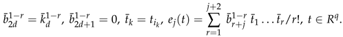
 where here and below, we use the tensor summation convention of implicitly summing each over its range . For example
 where the rth Edgeworth coefficient, , is a function of the . One could use unsymmetrized . For example by (2) needs the cross term in . So we could use in . But as (3) below illustrates, there is a big advantage in making symmetric in using the operator that symmetrizes over . So the for that we need are

 These formulas are mostly new. The terms involving are given explicitly for the first time in Appendix A. By Withers and Nadarajah (2010), the distribution and density of of (6), can be expanded as

 is the multivariate Hermite polynomial. By Withers (2020), for ,


 for of (8). These give and , and so of (15) to . For for needed for when , see Appendix B. is just with replaced by of (19). For example,
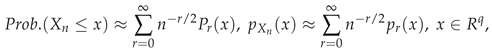
We call the partial moments of So by (15), the Edgeworth expansions to for the distribution and density of of (6) about those of , are given by
for of (8). These give and , and so of (15) to . For for needed for when , see Appendix B. is just with replaced by of (19). For example,
We call the partial moments of So by (15), the Edgeworth expansions to for the distribution and density of of (6) about those of , are given by
 for and of (18). Each has terms, but many are duplicates, as it is of great advantage to make symmetric in . The density of relative to its asymptotic value is
for of (17). So is a simple measure of the accuracy of the Central Limit Theorem (CLT) approximation. An exception is
for and of (18). Each has terms, but many are duplicates, as it is of great advantage to make symmetric in . The density of relative to its asymptotic value is
for of (17). So is a simple measure of the accuracy of the Central Limit Theorem (CLT) approximation. An exception is
Example 1.
If the distribution of is symmetric about w, then for r odd, and by (13), . So,

 since In this case is a measure of the accuracy of the CLT approximation. Also,
Example 2.
Let be the sample mean from a distribution with finite cross cumulants . Then , and only the leading coefficient in (5) is non-zero.
. For , the non-zero are
By (27)–(29), for and have only r terms.
NOTE 2.1.
For the univariate Hermite polynomial of (6), and
, we define the jth marginal Hermite polynomial as

Takemura and Takeuchi (1988) showed how to extend (4) to the multivariate case by replacing (8) by
It would very useful to obtain these multivariate explicitly. How does one extend the univariate formula for in terms of the ? Their §5 shows that the Cornish-Fisher expansions (4) are valid under the usual conditions for validity of the Edgeworth expansion (2).
NOTE 2.2.
Standard estimates have a natural extension to Type b estimates . These are estimates for which the cumulant expansion (5) is replaced by
Examples are 1-sided confidence interval limits. These have the form
where is a standard estimate and are smooth functions. See Withers and Nadarajah (2010) for more details.
3. Secondary or Derived Expansions
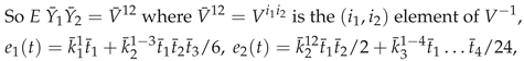
Let V have Hermitian form where .
As in (18)–(20), we use tensor summation and the bar notation, and
From the 2nd Edgeworth expansion in (15), it follows that for ,

 As is a linear combination of , we can write in terms of
This gives and of (1). So it gives to . For a sample mean, and for needed for , are given by Example 2.2. If , then for r odd, so that
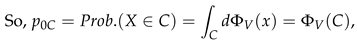
We now consider three such C. Ellipsoidal C. Take for some .
(We might choose u such that or .) of (8) is given by
As is a linear combination of , we can write in terms of
This gives and of (1). So it gives to . For a sample mean, and for needed for , are given by Example 2.2. If , then for r odd, so that
We now consider three such C. Ellipsoidal C. Take for some .
(We might choose u such that or .) of (8) is given by


 Similarly unless k is even and where are even integers and is a string of js of length k.
For of (13), set
where now for and so that are independent. Set
Similarly, using to mean a sum over distinct ,
of (9) is now given by (15), (17), (18). Note that
We can write in terms of
For of (6), set
where is an estimate , (empirical, semi-parametric, or parametric depending on the model used). So
the quantile of . It is often true that
(An exact confidence region for w is only possible if is normal: see 5.3.2 of Anderson (1958).) where and is a gamma random variable with mean . So if ,
with probability , and typically,
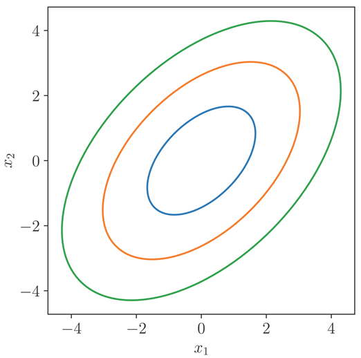
By way of illustration, Figure 3.1 plots the elliptical contours when , for when
So the asymptotic correlation of and is 1/2.
Figure 3.1: when for
courtesy of Dr Paul Teal:
 |
One can do similarly for , using and 2-dimensional slices of these ellipsoids. For related references on confidence regions, see Withers and Nadarajah (2012a).
The R functions. If then for , and
is given in Example 3.2 using a recurrence formula. (A simpler way is just to use (7).)
Now take . Then
 To get a recurrence formula for , set
This recurrence formula for of (20) gives
So we need . By Example 3.2,
Transforming to
where is the confluent or degenerate hypergeometric function: see 9.21 of Gradshteyn and Ryzhik (2000) and p504 of Abramowitz and Stegun (1964). Now suppose that . Then
where of (20) and is independent of .
By Theorem 2.2 of Withers and Nadarajah (2012a), for
Its extension to is given in §3 there for parametric and non-parametric models. Take . So . For and ,
(We might choose such that or .) For ,
So now is given by (16) and (17) in terms of these new . Similarly and are given by Example 3.1 with these new . So now we have of (9). If we choose , then
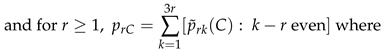
Take . So . This choice gives a set of q simultaneous intervals. For and
So for k odd. ( is no longer 0.) But each of those non-zero require q numerical integrations. Consider the case .
For more on these types of expansions and their inverses, see Hill and Davis (1968) and their simplifications given in §4–§5 of Withers and Nadarajah (2015). However in these papers the need to express results in terms of did not arise there. For the case of a sample mean with estimated covariance, it is possible to avoid the use of : see Xu and Gupta (2006).
4. The Distribution of for
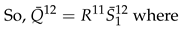
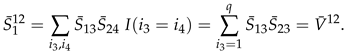
As above, we set . We now switch notation to

 So and are given by (33) with and 2:
and so on. The and needed here are given in Appendix B. Let us write the cumulant expansion (5) as
So The density of , , is given by (15) and (18) in terms of and of (18). As is symmetric,
for of (12)–(14). So is just with 1 and 2 reversed.
Then is given for by (27)–(29) in terms of
The needed in (3) for are as follows.
(15) and (18) now give the density of to . Set
The distribution of is given by (15) and (19) in terms of . is just above with replaced by of (5). That is,
(15) and (19) now give to for . For example for and , the values of are given in Example B.1. For , of (1) and (9) is given by replacing above by of (5) and of (Section 3). By §3,
These expressions can be read off those for in Appendix B. If , then for odd. For Examples 3.1 and 3.2, and of (4) is given by (15) in terms of . For this is given by (4). Let be a sample mean of a distribution with cumulants . By Example 2.2, for , and we need the following Edgeworth coefficients.
For is with superscripts 1 and 2 reversed. The needed for of (1) and (9) are those given above for . For a specific case of a bivariate sample mean, consider An entangled gamma model. Let be independent gamma random variables with means . For , set , and let be the mean of a random sample of size n distributed as . So, and where are independent gamma random variables with means . The rth order cumulants of are and otherwise . For example , and
So, Set Then V has correlation . This ranges from 0 at to 1 at So and are positively entangled. (For a negatively entangled example, replace by : the correlation is then . An extension to is ) For set
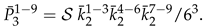
By Example 3.1, (so
Now consider the entangled exponential case . So , V and are given by (19),
So and are given by (33) with and 2:
and so on. The and needed here are given in Appendix B. Let us write the cumulant expansion (5) as
So The density of , , is given by (15) and (18) in terms of and of (18). As is symmetric,
for of (12)–(14). So is just with 1 and 2 reversed.
Then is given for by (27)–(29) in terms of
The needed in (3) for are as follows.
(15) and (18) now give the density of to . Set
The distribution of is given by (15) and (19) in terms of . is just above with replaced by of (5). That is,
(15) and (19) now give to for . For example for and , the values of are given in Example B.1. For , of (1) and (9) is given by replacing above by of (5) and of (Section 3). By §3,
These expressions can be read off those for in Appendix B. If , then for odd. For Examples 3.1 and 3.2, and of (4) is given by (15) in terms of . For this is given by (4). Let be a sample mean of a distribution with cumulants . By Example 2.2, for , and we need the following Edgeworth coefficients.
For is with superscripts 1 and 2 reversed. The needed for of (1) and (9) are those given above for . For a specific case of a bivariate sample mean, consider An entangled gamma model. Let be independent gamma random variables with means . For , set , and let be the mean of a random sample of size n distributed as . So, and where are independent gamma random variables with means . The rth order cumulants of are and otherwise . For example , and
So, Set Then V has correlation . This ranges from 0 at to 1 at So and are positively entangled. (For a negatively entangled example, replace by : the correlation is then . An extension to is ) For set
By Example 3.1, (so
Now consider the entangled exponential case . So , V and are given by (19),
 For and , the values of are given in Example B.1.
So if , then so that our measure of the accuracy of the CLT is for and
If , then , and our measure of the accuracy of the CLT is for , and for .
As in Example 2.1, suppose that the distribution of is symmetric about w. By (31),
and needed for (32) is with replaced by of (5). Now suppose that where and are independent copies of a random vector Then the cumulants of of odd order are zero, and the cumulants of even order are twice those of
Consider the case , the bivariate entangled gamma of Example 5.2. So , the odd cumulants of are zero, and the odd are zero. Denote of Example 3.2 as . Then
By Example 2.2, , where
Now consider the exponential case . So
So for Here we used the values of given in the example of Teal (2024). Takeuchi (1978) gave explicit expressions for the Cornish-Fisher expansion when .
5. Conclusions
Most estimates of interest are standard estimates, including functions of sample moments, like the sample correlation, and any smooth multivariate function of Fisher’s k-statistics: see Stuart and Ord (1991) for these. In §2 we gave the density and distribution of to , for any standard estimate, in terms of functions of the cumulants coefficients of (5), the coefficients of (11)–(14). §3 gave explicit detail when using the dual notation . §3 gave as examples Edgeworth expansions for the probability of lying in an ellipsoidal or hyperrectangular set.
6. Discussion
A good approximation for the distribution of an estimate, is vital for accurate inference. It enables one to explore the distribution’s dependence on underlying parameters. The analytic results given here avoid the need for simulation or jack-knife or bootstrap methods while providing greater accuracy than them. Hall (1992) used the Edgeworth expansion to show that the bootstrap gives accuracy to . Hall (1988) said that “2nd order correctness usually cannot be bettered”. But this is not true using these analytic results. Simulation, while popular, can at best shine a light on behaviour when there is only a small number of parameters.
Estimates based on a sample of independent but not identically distributed random vectors, are also generally standard estimates. For example for a univariate sample mean where has rth cumulant , then where is the average rth cumulant. For some examples, see Skovgaard (1981a, 1981b) and Withers and Nadarajah (2010, 2020). The last is for a function of a weighted mean of complex random matrices. It gives an application in electrical engineering to channel capacity for multiple arrays.
For conditions for the validity of multivariate Edgeworth expansions, see Skovgaard (1986) and its references.
Cornish and Fisher (1937) and Fisher and Cornish (1960) did not deal with the question of when these expansions diverge. We showed how to confront this in the numerical examples in Example 4.2 and Withers (1984).
Lastly we discuss numerical computation. We have used Teal (2024) for the numerical calculations in Example 4.2. One could also download R-4.4.1 for Windows and google for the routines needed. dmvnorm computes the density function of the multivariate normal specified by mean and co-variance matrix. Use mvtnorm for the multivariate normal. See also qmvnorm for quantiles. rmvnorm generates multivariate normal variables. Googling ’bivariate hermite polynomials r’ gives
One can then use install.packages("calculus"). However we have not used this route.
Some future directions.
1. Hill and Davis (1968) showed how to generalise the expansions of Cornish and Fisher about to expansions about an arbitrary continuous distribution. Their results are cumbersome as they involve partition theory. In Withers and Nadarajah (2015) we overcame this using Bell polynomials. It would be straightforward to apply these to expansions about in Example 3.1, to obtain the percentiles of and . However in the latter case we first need to derive the cumulant coefficients of from those of . This can be done by applying Withers (2024).
2. It would very useful to obtain the multivariate of (35) explicitly.
3. The multivariate expansions considered here have been about the multivariate normal. However as noted at the end of §1, expansions about other distributions can greatly reduce the number of terms in each and by matching bias and/or skewness. While this has been done for by Withers and Nadarajah (2011, 2012a, 2014) about Student’s distribution , the F-distribution, and the gamma, to date this has yet to be done for multivariate expansions about, for example, a multivariate gamma distribution.
4. The results given here are the first step for constructing confidence intervals and confidence regions. See Withers (1989).
5. The results here can be extended to tilted (saddlepoint) expansions by applying the results of Withers and Nadarajah (2010). These are very useful where convergence fails, that is, where the CLT cannot be improved upon, typically due to being in a tail. The tilted version of the multivariate distribution and density of a standard estimate are given by Corollaries 3, 4 there. Tilting was 1st used in statistics by Daniels (1954). He gave an approximation to the density of a sample mean. Jensen (1988) gave a univariate extension to where is the sum of i.i.d. observations and N is Poisson. The extension of the present results from to would be useful for both univariate and multivariate observations. For a review of references on tilting, see Withers and Nadarajah (2010).
6. Teal (2024) wrote a python program to obtain both analytic and numerical values of multivariate normal moments and multivariate Hermite polynomials when . It would be useful to have these extended to and 4. (The dual notation for and when or 4 is straightforward.)
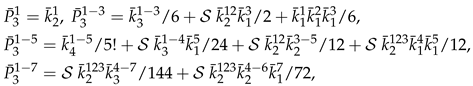
Appendix A: The Edgeworth coefficients needed for (11)
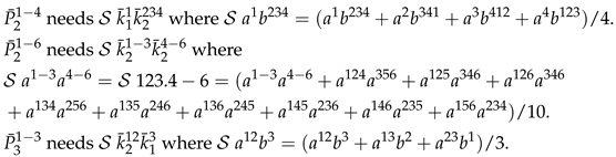
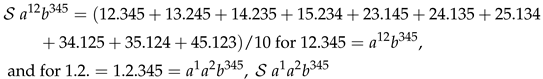
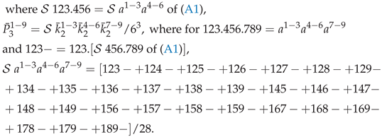
Here we give for the first time the symmetric form of the coefficients needed for (11) for , that is, for the Edgeworth expansions (15) to , using the symmetrising operator . They are given for by (12), and for by (13)–(14) and the following.


Appendix B: and of (2) for .
Here we give the bivariate normal moments of (1) and the bivariate Hermite polynomials of (2) for . These are needed for the Edgeworth expansions to .
The 1st 9 univariate Hermite polynomials are
 These are needed for of (2), (3), that is, for the univariate Edgeworth expansions to . See Stuart and Ord (1991).
Let be a q-variate normal random variable with mean , positive-definite covariance V, with density and distribution of (7). Set as in (8), so that Y has odd moments 0 and even moments

 where sums over the m permutations of giving distinct terms. For example,
Teal (2024) has written a python program to obtain the bivariate moments using (A2). Let be the multivariate Hermite polynomial is defined by of (20), (21). For is given by (8)–(26). In these expressions can be replaced by any integers in . For example
Now consider the bivariate case, and denote the moments of Y by
Two special cases are
The needed here are those up to order
For example to derive from of (A2), replace by 1 and by 2. can be read off using symmetry. For example . Formulas for the general were given by Isserlis (1918) and Withers (2). By (Section 4),
This is the formula used in Teal (2024) to obtain bivariate Hermite polynomials. is said to be of order. Most of those of order up to are needed to expand the density of to , but not those of order 8, (nor those of order 6 if the distribution of is symmetric about w). But we include them here for completeness.
where sums over the m permutations of giving distinct terms. For example,
Teal (2024) has written a python program to obtain the bivariate moments using (A2). Let be the multivariate Hermite polynomial is defined by of (20), (21). For is given by (8)–(26). In these expressions can be replaced by any integers in . For example
Now consider the bivariate case, and denote the moments of Y by
Two special cases are
The needed here are those up to order
For example to derive from of (A2), replace by 1 and by 2. can be read off using symmetry. For example . Formulas for the general were given by Isserlis (1918) and Withers (2). By (Section 4),
This is the formula used in Teal (2024) to obtain bivariate Hermite polynomials. is said to be of order. Most of those of order up to are needed to expand the density of to , but not those of order 8, (nor those of order 6 if the distribution of is symmetric about w). But we include them here for completeness.
We can write in terms of of (A5) and :
 These are actually simpler formulas than their univariate forms because of the use of . The other up to order 9 are
The method of proof is illustrated as follows
Now expand the 2nd term to get
Similarly for , expand
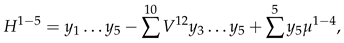
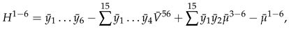
The above formulas for can be called their short form as each uses . The explicit form when of (A7) is substituted can be called its long form. Our short forms for were checked against the long forms given by Teal (2024). Here is a selection of his results for comparison.
For example the short and long forms for have 5 and 10 terms, and those for have 8 and 13 terms.
These are actually simpler formulas than their univariate forms because of the use of . The other up to order 9 are
The method of proof is illustrated as follows
Now expand the 2nd term to get
Similarly for , expand
The above formulas for can be called their short form as each uses . The explicit form when of (A7) is substituted can be called its long form. Our short forms for were checked against the long forms given by Teal (2024). Here is a selection of his results for comparison.
For example the short and long forms for have 5 and 10 terms, and those for have 8 and 13 terms.
Take of (19). Then
So if then
If , then
These results were computed by Teal (2024), using (A6), and are used in Example 4.2.
Appendix I Code for Bivariate Normal Moments and Bivariate Hermite Polynomals
2.12.25 ex Paul: Here is a latex file which has all the moment evaluations and Hermite polynomial evaluations corrected.
The code to generate it is publicly available at https://github.com/paultnz/bihermite/blob/main/hermite8.py so you can refer to it in the paper and hopefully that will satisfy your reviewers. It can be applied to any values of the subscripts and any values of mu02, mu20, mu11, y1 and y2.
#!/usr/bin/env python3
#
# Paul Teal - pault@nmr.nz
# Thursday 7 November, 2024
# Monday 2 December, 2024
from itertools import product
from math import comb
from fractions import Fraction as fr
import sympy as sy
import re
def split_string(str,maxlen=100):
# This is just for limiting the maximum length of latex display lines
sections = re.split(r’(?=[+-])’,str)
result = []
current = ’’
for ss in sections:
current += ss
if len(current) >= maxlen:
result.append(current)
current = ’’
if current:
result.append(current)
return result
def mup(Elist):
# recursive function for evaluating moments
if Elist == []:
return 1
if Elist == [1,1]:
return mu20
if Elist == [2,2]:
return mu02
if Elist == [1,2]:
return mu11
if Elist == [2,1]:
return mu11
Rout = 0
for ii in range(len(Elist)-1):
left = mup([ Elist[ii], Elist[-1] ])
right = mup(Elist[:ii] + Elist[ii+1:-1])
Rout += left * right
return Rout
def sub2(sb1,sb2):
return mup([1] * sb1 + [2] * sb2)
def biHermite(n, m, y1=0, y2=0, mu=0):
# Generate terms for (y1 + j*Y1)^n
terms1 = []
for k in range(n + 1):
terms1.append((comb(n, k) * (1j ** k), n-k, k))
# Generate terms for (y2 + j*Y2)^m
terms2 = []
for k in range(m + 1):
terms2.append((comb(m, k) * (1j ** k), m-k, k))
# Combine terms from both expansions
terms = 0
for (coef1, a_pow, b_pow), (coef2, c_pow, d_pow) in product(terms1, terms2):
coef_all = coef1 * coef2
if coef_all.imag == 0: # ignore imaginary
coef_all = int(coef_all.real)
combined = coef_all * y1**a_pow * y2**c_pow * sub2(b_pow,d_pow)
terms += combined
return terms
if __name__ == "__main__":
# Example usage: the first iteration is purely symbolic, then the
# second and third use some specific values
for loop in range(3):
if loop==0:
mu20, mu02, mu11, y1, y2= sy.symbols(’mu20 mu02 mu11 y1 y2’)
elif loop==1:
#override symbols with specific values
mu20 = fr(2,3); mu02 = fr(2,3); mu11 = -fr(1,3); y1 = fr(1,3); y2 = fr(1,3)
elif loop==2:
y1 = fr(2,3); y2 = fr(2,3)
if loop<2:
# Print values of mu
print(’\\begin{align*}’)
for mn in range(4,9+1,2):
for m in range( (mn+2)//2):
n = mn-m
l2 = sub2(m,n)
print(f’\\mu_{{{m}{n}}} =& ’ + sy.latex(sy.simplify(l2)) + ’\\\\’)
print(’\\end{align*}’)
print(’%%%%%%%%%%%%%%%%%%%%%%%%%%%%%%%%%%%%%%%%%%%%%%%%%%%%%%%%%%%%%%%’)
print(’\\begin{align*}’)
for nm in range(1,10):
for m in range(0,(nm+2)//2):
n = nm - m
result = sy.expand(biHermite(n, m, y1, y2),mul=True)
la = sy.latex(result)
print(f’H_{{{n}{m}}} =&’,sep=’’,end=’’)
if not result.free_symbols:
print(f’{la} \\approx {result.evalf():.4f}\\\\’)
else:
lines = split_string(la,150)
for line in lines[:-1]:
print(line,’\\\\& ’)
print(lines[-1],’\\\\’)
print(’\\end{align*}’)
print(’%%%%%%%%%%%%%%%%%%%%%%%
References
- Abdel-Wahed, A.R. and Winterbottom, A. (1983) Approximating posterior distributions of system reliability. The Statistician, 32, 224–228. [CrossRef]
- Abramowitz, M. and Stegun, I. A. (1964) Handbook of mathematical functions. U.S. Department of Commerce, National Bureau of Standards, Applied Mathematics Series 55.
- Anderson, T. W. (1958) An introduction to multivariate analysis. John Wiley, New York.
- Comtet, L. Advanced Combinatorics; Reidel: Dordrecht, The Netherlands, 1974.
- Cornish, E.A. and Fisher, R. A. (1937) Moments and cumulants in the specification of distributions. Rev. de l’Inst. Int. de Statist. 5, 307–322. Reproduced in the collected papers of R.A. Fisher, 4. [CrossRef]
- Fisher, R. A. and Cornish, E.A. (1960) The percentile points of distributions having known cumulants. Technometrics, 2, 209–225. [CrossRef]
- Gradshteyn, I.S., and Ryzhik, I.M., (2000) Tables of integrals, series and products. 6th edition. Academic Press, New York. The generalized hypergeometric function is defined in §9.14.
- Gradshteyn, I.S., and Ryzhik, I.M., (2000) Tables of integrals, series and products. 6th edition. Academic Press, New York. The generalized hypergeometric function is defined in §9.14.
- Hill, G.W. and Davis, A.W. (1968) Generalised asymptotic expansions of Cornish-Fisher type. Ann. Math. Statist., 39, 1264–1273. [CrossRef]
- On a formula for the product-moment coefficient of any order of a normal frequency distribution in any number of variables. Biometrika, 12, 134–139. JSTOR 2331932.
- Jensen, J.L. (1988) Uniform saddlepoint approximations, Adv. Appl. Prob. 20, 622-634.
- Simonato, J.G. (2011) The performance of Johnson distributions for computing value at risk and expected shortfall. Journal of Derivatives (19) 7–24. [CrossRef]
- Skovgaard, I.M. (1981a) Edgeworth expansions of the distributions of maximum likelihood estimators in the general (non i.i.d.) case. Scand. J. Statist., 8, 227-236.
- Skovgaard, I. M. (1981b) Transformation of an Edgeworth expansion by a sequence of smooth functions. Scand. J. Statist., 8, 207-217.
- Skovgaard, I. M. (1986) On multivariate Edgeworth expansions. Int. Statist. Rev., 54, 169–186. [CrossRef]
- Stuart, A. and Ord, K. (1991). Kendall’s advanced theory of statistics, 2. 5th edition. Griffin , London.
- Takemura, A. and Takeuchi, K. (1988) Some results on univariate and multivariate Cornish-Fisher expansions: algebraic properties and validity. Sankhya, Series A50, 111–136.
- Takeuchi, K. (1978) A multivariate generalization of Cornish-Fisher expansion and its applications. (In Japanese.) Keizaigaku Ronshu, 44, (2), 1–12.
- Teal, P. (2024) A code to calculate bivariate Hermite polynomials.https://github.com/paultnz/bihermite/blob/main/bihermite.py Its input is V11,V12,V22 and y1,y2, not V11,V12,V22 and x1,x2.
- TianLi, S., ShuNing, W. and WeiLian, A. (2009) GPS positioning accuracy estimation using Cornish-Fisher expansions. International Conference on comms. and mobile computing, IEEE Computer Soc., 152–155.
- Winterbottom, A. (1980) Asymptotic expansions to improve large sample confidence intervals for system reliability. Biometrika, 67, 351–357. [CrossRef]
- Winterbottom, A. (1984) The interval estimation of system reliability component test data. Operations Research, 32, 628–640. [CrossRef]
- Withers, C.S. (1984) Asymptotic expansions for distributions and quantiles with power series cumulants. Journal Royal Statist. Soc. B, 46, 389–396. Corrigendum (1986) 48, 256. For typos, see p23–24 of Withers (2024). [CrossRef]
- Withers, C.S. (1989) Accurate confidence intervals when nuisance parameters are present. Comm. Statist. - Theory and Methods, 18, 4229–4259. [CrossRef]
- Withers, C.S. (2000) A simple expression for the multivariate Hermite polynomials. Statistics and Prob. Letters, 47, 165–169. [CrossRef]
- Withers, C.S. (2024) 5th-Order multivariate Edgeworth expansions for parametric estimates. Mathematics, 12,905, Advances in Applied Prob. and Statist. Inference. https://www.mdpi.com/2227-7390/12/6/905/pdf. [CrossRef]
- Withers, C.S. (2025) New methods for multivariate normal moments. Stats. 8(2), 46. [CrossRef]
- Withers, C.S. and Nadarajah, S.N. (2009) Charlier and Edgeworth expansions via Bell polynomials. Probability and Mathematical Statistics, 29, 271–280. For typos, see p24–25 of Withers (2024).
- Withers, C.S. and Nadarajah, S. (2010) Tilted Edgeworth expansions for asymptotically normal vectors. Annals of the Institute of Statistical Mathematics, 62 (6), 1113–1142. [CrossRef]
- Withers, C.S. and Nadarajah, S. (2011) Generalized Cornish-Fisher expansions. Bull. Brazilian Math. Soc., New Series, 42 (2), 213–242. [CrossRef]
- Withers, C.S. and Nadarajah, S.N. (2012a) Improved confidence regions based on Edgeworth expansions. Computational Statistics and Data Analysis, 56 (12), 4366–4380. [CrossRef]
- Withers, C.S. and Nadarajah, S.N. (2012b) Cornish-Fisher expansions about the F-distribution. Applied Mathematics and Computation, 218 (15), 7947–7957. [CrossRef]
- Withers, C.S. and Nadarajah, S. (2014) Expansions about the gamma for the distribution and quantiles of a standard estimate. Methodology and Computing in Applied Prob., 16 (3), 693-713. [CrossRef]
- Withers, C.S. and Nadarajah, S. (2015) Edgeworth-Cornish-Fisher-Hill-Davis expansions for normal and non-normal limits via Bell polynomials. Stochastics An International Journal of Probability and Stochastic Processes, 87 (5), 794–805. [CrossRef]
- Withers, C.S. and Nadarajah, S. (2020) The distribution and percentiles of channel capacity for multiple arrays. Sadhana, SADH, Indian Academy of Sciences, 45 (1), 1–25. [CrossRef]
- Xu, J. and Gupta, A.K. (2006) Improved confidence regions for a mean vector under general conditions. Computational Stat. and Data Analysis, 51 1051-1062. [CrossRef]
- Zhang, L., Mykland, P.A. and Ait-Sahalia, Y. (2011) Edgeworth expansions for realised volatility and related estimators. Journal of Econometrics (160) 190–203. [CrossRef]
Disclaimer/Publisher’s Note: The statements, opinions and data contained in all publications are solely those of the individual author(s) and contributor(s) and not of MDPI and/or the editor(s). MDPI and/or the editor(s) disclaim responsibility for any injury to people or property resulting from any ideas, methods, instructions or products referred to in the content. |
© 2025 by the authors. Licensee MDPI, Basel, Switzerland. This article is an open access article distributed under the terms and conditions of the Creative Commons Attribution (CC BY) license (http://creativecommons.org/licenses/by/4.0/).
Copyright: This open access article is published under a Creative Commons CC BY 4.0 license, which permit the free download, distribution, and reuse, provided that the author and preprint are cited in any reuse.


