
Submitted:
16 July 2025
Posted:
17 July 2025
You are already at the latest version
Abstract
Remaining useful life (RUL) estimation is an integral part of prognostics and health management of engineering systems. Using RUL estimation, failures could be detected and maintained before they occur. Advancements in sensor technology permitted monitoring the health state of engineering systems producing a lot of data. This data is utilized for building data-driven RUL estimation models. Today both in practice and literature data-driven models for RUL estimation are very popular since the construction of these models usually does not require domain knowledge, it is easy to adapt existing models for different engineering systems and provide accurate estimations. Artificial Neural Networks are widely used in data-driven computing for modeling nonlinear regression and dynamic systems. Nonlinear Auto-regressive neural network with eXogenous inputs (NARX) model is used for dynamic modeling and multi-step long-term forecasting. NARX makes predictions by iteratively simulating the dynamic behavior of underlying nonlinear time series. Since the system monitoring data are dynamic nonlinear time series, this feature of NARX makes it a suitable model for RUL estimation. In this study, a genetic algorithm-based series-parallel mode NARX (GABPM-NARX) model is proposed for RUL estimation. The proposed approach is applied to the C-MAPSS dataset from the NASA data repository. The results of the analysis are satisfactory showing that the proposed parallel mode NARX model is a promising method for RUL estimation.
Keywords:
remaining useful life
; convolutional neural network
; NARX model
; prognostics
; turbofan engine
1. Introduction
Both in production and service industries, prognostics, and health management (PHM) of engineering systems is very important for safe, reliable, and cost-efficient operation. Failure of the equipment during operation may have serious consequences. In terms of safety, there may be serious injuries, loss of life, and damage to the environment. In terms of financial losses, companies incur corrective maintenance costs (which are usually much higher than preventive maintenance costs) and opportunity costs due to the stoppage of production or services. Prognostics deals with estimating the time to failure of a system which is called as remaining useful life (RUL) in the literature [1]. Estimation of an engineering system’s RUL enables a company to plan the maintenance workforce and spare part supply resulting in more effective and efficient health management.
Prognostics models for RUL estimation are classified as physics-based, data-driven, and hybrid models [2]. Physics-based models express the system degradation by mathematical equations exploiting the system knowledge [3]. This approach requires expertise in system structure and dynamics, and it could be very difficult to construct mathematical equations representing the system degradation. Also, these models are system-specific so they cannot be generalized for other systems. Data-driven models do not require expertise in the system domain, and they can be generalized for other systems. These approaches utilize sensor technology to collect data that reflects the system deterioration. In the last two decades data-driven methods have been used extensively in PHM [4,5,6,7,8,9,10,11,12,13,14,15,16,17,18,19,20]. The downside of the data-driven approaches is that they require a lot of data. In the case of limited data, hybrid models can be used for estimation of RUL. Hybrid models usually utilize data driven modelling for estimating the system state based on the sensor measurements (measurement model) then system degradation is expressed by physics-based models to estimate the RUL (degradation model) [21,22]. For the review of the topic see [22,23,24]. In this manuscript for a sufficient data case, a new data-driven methodology is proposed for the estimation of RUL utilizing Nonlinear Auto Regressive neural network with eXogenous inputs (NARX). NARX is a special kind of recurrent neural network. The proposed methodology is applied to NASA C-MAPSS data which is a benchmark dataset from the NASA data repository [25]. Although the data belongs to turbofan engines, the developed methodology can be generalized for any system.
Artificial Neural Networks (ANNs) are one of the data-based prognostics commonly used in literature. ANNs are computational algorithms inspired by the complex functionality of the human brain, where interconnected neurons process information in parallel [26]. These models do not use traditional statistical methods, but they are built as massively parallel networks, and trained to predict outputs [27]. ANNs are used effectively in modeling nonlinear relations and dynamical systems [28]. ANN is a very successful instrument in modeling the relationship between inputs and outputs in complex systems where the obvious exact relationship between inputs and outputs in the data is unknown [29]. With its ability to learn effectively from supervised and unsupervised input data, it can be applied to various fields such as modeling, time series analysis, pattern recognition, signal processing, and control [30,31]. ANNs can be divided into two categories: feedforward neural networks (FNNs) and recurrent neural networks (RNNs) [32]. The difference between them is that an RNN has a feedback mechanism between neurons, while an FNN does not. There would be one or more feedback connections between RNN neurons. The feedback mechanism can be quite diverse, from one neuron feeding back to another, a neuron feeding back to more than one neuron, more than one neuron feeding back to a neuron, or even a neuron feeding back to itself. The state of a network at any given moment depends on its previous state, which is achieved by feedback [33]. RNNs make predictions with dynamic modeling by iteratively simulating the dynamic behavior underlying nonlinear time series with an autonomous system with multi-step long-term predictions [34]. This structure is very useful for the analysis of dynamic systems. Since an engineering system and the sensors that monitor its state have a very dynamic and complex relation, we propose a new RUL prediction methodology based on the NARX model. The contributions of this paper can be summarized as follows:
- The predictive power of the NARX for solving dynamic and complex problems is recognized and proposed as a promising new model for the estimation of RUL.
- The hidden layer size and the delay size are two important parameters for the NARX architecture. In literature, as of our knowledge, these parameters are determined by trial. We utilized the genetic algorithm (GA) to determine the optimal values for hidden layer size and delay size, so the proposed model is called the genetic algorithm-based series-parallel mode NARX (GABPM-NARX) model.
- The developed GA fitness function for parameter optimization is independent of the model form so that it could be used for optimizing the parameters of other data-driven RUL estimation models in the literature.
- The proposed GABPM-NARX framework exhibits superior prediction accuracy in Remaining Useful Life (RUL) estimation compared to existing methodologies in literature. Owing to its robust performance and generalization capabilities, this method is poised to play a significant role in future RUL prediction research and applications. Its distinctive architecture empowers the model to extract enriched representations from complex degradation patterns, positioning GABPM-NARX as a promising benchmark in prognostics and health management.
To decrease the negative effect of the sensor noise on the performance of the NARX model, median filtering is utilized. The proposed median filtering approach also can be utilized in the data preparation stage for other existing models in literature.
The remainder of this paper is organized as follows. Section 2 provides a review of the literature. For fast access to concise information, the most crucial aspects of literature are summarized in a table. Section 3 provides a brief review of the NARX model and GA as preliminary. A detailed explanation of the proposed methodology is given in Section 4. A numerical experiment of the proposed methodology run on the C-MAPPS data set and given in Section 5. Finally, Section 6 provides conclusions.
2. Related Work
This section provides a concise review of the current literature on RUL estimation that utilizes the NASA C-MAPSS turbofan engine data. We decided to give the literature review in a table format since it gives the most important information in a concise form and makes the comparison of literature easy (Table 1). The papers in Table 1 are compared in terms of the data preprocessing steps, the framework used in modeling, and the metrics used for performance evaluation. In addition, the papers in the literature were analyzed in terms of keywords by years in Figure 1. The network density diagram shows that the most frequently used keywords in the papers are remaining useful life, deep learning, prognostics and health management, prognostics, C-MAPSS, predictive maintenance, prediction, Long Short-Term Memory (LSTM), turbofan engine, convolutional neural network (CNN), and machine learning.
3. Preliminary
3.1. NARX Model
The Nonlinear Auto Regressive neural network with eXogenous inputs (NARX) model is a type of RNN that can capture the nonlinear and dynamic relationships between input and output variables. In time series it is natural to have long-term dependencies. Auto Regressive part of the NARX allows the output depend not only on the previous outputs but also on the current and past inputs. Due to this feature, NARX is successful in predicting time series [6,40,41]. The NARX model can be used also for system identification [42], control [43] and signal processing [44] applications. It can handle complex data with high accuracy and robustness. The ability of the NARX model to maintain predictive or actual time series of historical data affects its performance [45]. NARX converges faster than other neural network models, generalizes well, and shows effective learning [46]. In addition, the NARX model belongs to the model class that is computationally equivalent to Turing machines [47].
The basic element of any kind of ANN is a neuron. The structure of a neuron is shown in Figure 2. Here the neuron has input arcs, and each arch has a weight associated with it. Weighted input signals are combined and a bias added to the sum to obtain intermediate output . The final output is obtained by applying an activation function to. The NARX model is formed by the interconnected layers of neurons in a special recurrent architecture.
For a general NARX model, input and output relation can be defined by the formula in Equation (1):
While represents either real outputs or network outputs depending on the architecture, represents network inputs. Time delay parameters expressed by and respectively indicate the number of past outputs and past inputs to be used for feedback, and denotes the discrete time step. Thus, the feedback and input layers are time-delayed and contain historical data [47]. The network structure of a general NARX model is shown in Figure 3. The model comprises an input layer, a hidden layer, and an output layer.
NARX models have two different architectures: series-parallel (also called as open loop) (Figure 4a) and parallel (also called as closed loop) architecture (Figure 4b). In the series-parallel architecture, the real output values are given as additional inputs whereas in the parallel architecture predicted output values are given as additional inputs. Formulation of series-parallel and parallel architecture is given in Equations (2) and (3) respectively:
In Equation (2) is the real output value at time and in Equation (3) is the prediction of the output for time at time . is input values, and is the mapping function. As it can be seen from Equation (2), in the series-parallel architecture is predicted using past real output values with time delay and input values with time delay . As opposed to in parallel architecture is predicted using past predicted output values with time delay and input values with time delay as shown in Equation (3). The series-parallel and parallel architectures are shown in Figure 4.
The advantage of the series-parallel architecture is that the accuracy of the prediction increases by the use of the actual output values also as inputs. For example, if the problem is to estimate next year's wheat yield, past years' yield values can be used. RUL estimation appropriate NARX architecture is series-parallel architecture.
3.2. Population-Based Metaheuristics Method: Genetic Algorithm (GA)
The genetic algorithm (GA) is a population-based metaheuristic search algorithm inspired by evolutionary theory [48,49]. It focuses on the selection of suitable individuals by natural selection from a population of characters (a set of potential solutions). This process is based on transferring the good genes of the current generation to the future generations so that the chromosomes of future individuals are shaped accordingly. GA iteratively constructs the chromosome structures of future individuals from the good genes in the chromosome structures of ancestors. It is a good method for solving difficult combinatorial optimization problems. In this way, GA optimizes the model expressed around a problem-specific fitness function. GA consists of a population with a character set, control parameters, fitness function, crossover, mutation, selection, and coding operations [50]. The features of GA use a solution space in the search, provide probabilistic transitions, work with a parameter set, and focus on the return of the fitness function [51].
GA uses crossover and mutation functions to generate appropriate chromosome structures that optimize the fitness function. Crossover is the function to generate daughter solutions, that is, new chromosomes, by randomly selecting a crossover point from two parent solutions. Crossover GA is also one of the most important functions for generating suitable new chromosomes. The mutation function, on the other hand, ensures that the algorithm does not get stuck in the local optimal solution, so that genetic diversity is preserved, and the valuable information contained in the chromosomes is not prematurely lost (Grossmann & Sargent, 1978).
4. Proposed methodology for RUL estimation
4.1. Flowchart of the Proposed Methodology for RUL Estimation
The flowchart of the proposed methodology for RUL estimation is shown in Figure 5. First, feature selection is performed based on the raw data set to identify the most relevant features that give information about the degradation of the system. For this purpose, graphical and correlation analyses are utilized. The selected features are normalized using the z-score normalization method. Then, the RUL column is rectified with the piece-wise linear function. Finally, the noise in the data is removed by the median filter method. These steps are explained in detail and exemplified in the numerical example section. The processed training set is transferred to the NARX model. The parallel architecture is selected, and the GA is used to determine the number of hidden layers in the model architecture. Finally, the trained NARX model is used for the estimation of RUL values.
4.2. Genetic Algorithm-Based Series-Parallel Mode NARX Model (GABPM-NARX)
Mathematical formulation of the parallel mode NARX model is developed hierarchically starting from the neuron which is the basic element of the architecture. Let us assume that the architecture has m hidden layer, and each layer has s neurons. The formulation of neuron of hidden layer for time is given in Equation (4).
In Equation (4), is the logistic activation function and its formulation is given in Equation (5). and represents the indexes for neuron and exogenous variable sizes respectively. is the input bias. is the value of exogenous variable at time and are the input layer weight of it at neuron . represents the time delayed value of exogenous variable and represents time delayed estimated output. and represent the input layer weights for time delayed exogenous variable and time delayed estimated output, respectively.
A hidden layer is composed of s neurons. The formulation of hidden layer at time is given in Equation (6).
Here is the weight of neurons. Finally, the output layer combines all the hidden layers and it is formulation given in Equation (7).
Here is the activation function for the output, which is . The output bias is and the output layer weights are . Inserting Equations (4) and (6) in Equation (7), we obtained Equation (8) which is the expression of the parallel mode NARX model.
Hidden layers learn the relationship between inputs and output. Therefore, the size of hidden layers affects the performance of the NARX model. One of the other important parameters is the delay size that defines the auto-regressive part. In previous studies that utilized NARX model, the hidden layer and the delay size were determined manually by trial and error [45,52]. In this study, GA is used for determining the optimal/near-optimal values of these parameters.
To perform the optimization by GA, a special fitness function is constructed. The fitness function of GA is called as , and its calculation formula is expressed in Equation (9).
Here, and are the predicted RUL and actual RUL values of the row of the training dataset, respectively. is the total number of samples in the training data. is found utilizing Levenberg-Marquardt learning algorithm which is the popular algorithm in literature [53,54].
Once the GABPM-NARX model is constructed the training data is fed into the model to learn the relation between inputs and output. Then trained model can be used for estimating RUL values.
5. Experimental Study
5.1. C-MAPSS Dataset
The dataset provides the run-to-failure trajectories of a fleet of turbofan engines. It is generated utilizing the Commercial Modular Aero-Propulsion System Simulation (C-MAPSS) model developed at NASA [25], [55]. The dataset includes four different subsets (FD001, FD002, FD003, and FD004) that are simulated under different combinations of operating conditions and failure modes. Table 2 provides detailed information on the data subsets. The data subsets consist of multivariate time series that record the information in the sensor channels to be able to characterize the failure evolution. Each subset is divided into training and test sets. The engines always run normally at the beginning of the time series and develop a fault at some point during the series. In the training set, the error grows until it becomes a system error. In the test set, the time series ends sometime before the system failure. The goal is to estimate the RUL on the C-MAPSS test set. In addition, a vector of actual RUL values is provided for the test data. The data is presented in 26 columns. In the dataset column 1 gives the engine ID number, column 2 gives the running cycle, column 3-5 gives operational settings, and column 6-26 gives the 21 different sensor measurements. Each row of the data set is a snapshot of the data obtained during a single processing cycle.
A diagram of the turbofan engine is shown in Figure 6. Key components include a fan, low-pressure compressor (LPC), high-pressure compressor (HPC), fuel oil, high-pressure turbine (HPT), low-pressure turbine (LPT), and nozzle. Sensors monitor the health of the key components of the turbofan engine. The description of the 21 sensors is shown in Table 3.
5.2. Data Preparation
Data preparation steps in order are feature selection, normalization, RUL label rectification, and noise-cleaning. Details of these steps are given below.
5.2.1. Feature Selection-Graphical and Correlation Analysis
The measurement data of some sensors do not change at all during the life of the turbofan engine or change around fixed values, so they do give none or very little information about the health state of the engine. Including irrelevant sensors in the study would increase variation and the noise thereby decreasing the prediction accuracy. These sensors should be removed by feature selection methods. In this study, feature selection is performed by graphical and correlation analysis.
Figure 7 gives examples (due to space limitation) of time series graphs showing the different behaviors of the sensor measurements. Measurements of sensors 1, 5, 10, 16, 18, and 19 stay constant through the whole engine life as in Figure 7a. Measurements of sensor 6 change between 21.6 and 21.61 without any trend and is given in Figure 7b. Measurements of sensors 2-4, 7-10, 11-15, 17, and 20-21 show a trend as in Figure 7c.
Pearson correlation coefficient analysis is a filtering method for determining exclusions from a dataset based on the degree of correlation. Pearson correlation coefficient measures the linear relation between two variables and is expressed in Equation (10). As gets closer to +1 positive linear relation between two variables increases, as gets closer to -1 negative relation between two variables increases, and as r get closer to 0 relation between two variables decreases. Table 4 gives Pearson correlation coefficients between RUL and each sensor. Table 4 supports the results of the graphical analysis. The correlation between RUL and constant sensors is zero. The correlation between RUL and Sensor 6 is -0.11. Correlation between RUL and sensors with a trend ranging from -0.78 to 0.75. As a result of two analyses, sensors 2,3,4,7,8,9,11,12,13,14,15,17,20, and 21 are selected as features.
The age of an engine (the running cycle) also provides important information for the estimation of the RUL. The Pearson correlation coefficient between RUL and the running cycle is calculated as -0.746 indicating that the running cycle should be added to the feature set. As a result, the feature set included 14 selected sensor values and the running cycle.
5.2.2. Z-Score Normalization
The scale of the measurement values of the sensors are different from each other, and this will negatively impact the model training process. Therefore, the sensor data must be normalized. There are many ways to normalize variables, in this study z-score normalization, the most popular technique, was utilized [56,57]. The formula of z-score normalization is shown in Equation (11) [58]. Here is the measurement of sensor, is the mean of sensor measurements, is the corresponding standard deviation, and is the normalized value of the measurement of sensor.
5.2.3. Piece-Wise Linear Function
RUL labels for the training dataset start with maximum life of the engines and decrease by one for each flight cycle until the failure occurs. When failure occurs, the RUL label becomes zero. Accordingly, the shape of RUL is a time-decreasing linear function. But in practice, the deterioration of the system is almost constant at the beginning, and it starts decreasing with the first signs of engine degradation. Reflecting on this observation, a piece-wise linear RUL function has been proposed in [59] and adopted in the literature [15,60,61]. RUL label rectification formula is expressed in Equation (12). Here represents the constant RUL value in early life. In this study is set to 125 cycle as suggested in [62]. Based on this value, graph of the piece-wise linear RUL function is shown in Figure 8.
5.2.4. Noise Cleaning with Median Filter
Noise in the sensor measurements decreases the model performance. Median filtering, developed by [63], is a useful non-linear signal processing technique for regulating noise in data. It is a popular filtering method in image processing [64,65,66]. In image processing, the median filter is applied to the data in sliding windows of odd size. By filtering the center of the window is replaced by the median of the window. Figure 9 shows the a median filter and a mean (smoothing) filter applied to discrete step function, a ramp function, a pulse function, and a triangle function with a window of five pixels [67]. It can be seen from the Figure 9 that median filter does not affect the step function and ramp functions. For the pulse functions, pulses whose periods are less than one-half of the window width, are suppressed. For the triangle function it flattens the peak of the triangle.
In this study, median filtering is used to regulate the noise in FD001 dataset. Window size is taken as a whole data size for not losing important information. As an example, Figure 10 shows the signal distribution for Sensor 3 and Sensor 15 with and without median filter. It can be seen that median filter smooths the noise without changing the shape of the signal trajectories.
5.3. Experimental Setup
Let us summarize the preparation of FD001 dataset, given in section 5.2. In the first step sensors 2,3,4,7,8,9,11,12,13,14,15,17,20, and 21 are selected using graphical and correlation analysis. Based on its high correlation the running cycle is added to the feature set. Time series plots of the selected sensors are given in Figure 11 In the second step normalization is performed applying the z-score method to the sensors. The running cycle is not normalized. In the third step RUL labels are rectified by setting as 125 flight cycle. In the fourth step median filtering is utilized to clean the noise in the sensor data. Although there is a separate training data set, to evaluate the internal performance of the model testing data set is divided into 5% validation and 5% testing in the fifth step.
Time delay size is determined by examining the sensor values. The sensors values are approximately similar in the 4 cycle-time windows, as shown in Figure 12. From another point of view, when examined within the framework of maintenance logic, a time period of about 4 cycles can inform the malfunction.
Hidden layer size and delay size determined by the GA using the fitness function given in Equation (9). The GA parameters are expressed in Table 5.
As stated in Section 4.2, Levenberg-Marquardt learning algorithm is used for the estimation of RULiestimated_sample values in Equation (9). Figure 13 shows the fitness function value of the GA. In the initial generations, there was a rapid improvement in fitness function, and in the next generations, appropriate value was obtained with minimal improvements. Optimum value of hidden layer size determined as 10 and delay size determined as 4.
Next parallel NARX model is constructed. Model parameters of the NARX Model (time delay size, size of hidden layer, type of learning algorithm, and error formula) are given in Table 6.
Using 10 hidden layers, the proposed GABPM-NARX model is constructed, and its architecture is given in Figure 14.
Once the GABPM-NARX model is constructed, it is trained using three different learning algorithms, the Levenberg-Marquardt Method, Scaled Conjugate Gradient Method, and Bayesian Regulation Method. The best results were obtained when the Levenberg-Marquardt Method was used, and only the result of this model is given below.
5.4. Evaluation of Training Process
The training data set can be represented in matrix format as follows. There are 20631 rows of training data belonging to 100 engines. Each row represents one flight cycle. The values of 14 sensors are selected as features. Let be the lifetime of the system , . The maximum lifetime is 362 flight cycles belonging the engine number 69 and the minimum lifetime is 128 flight cycles belonging to engine 39. Sensor measurements of system during its lifetime can be represented by the matrix , . Here is the vector of sensor measurements for system during its lifetime . So, the whole data set is a matrix with dimension 15
20631. The dataset was partitioned into training, validation, and test subsets, with respective allocations of 60%, 20%, and 20%.
Using this data, the GABPM-NARX model is trained using the Levenberg-Marquardt algorithm to learn the relation between inputs and output. The regression determination coefficient of the simple linear regression model between output values and target values can be used as the first metric to evaluate the success of the model training process. As is well known, R can take values in the interval [0,1]. The closer the value of R to 1, the better the training process is. The regression results are shown in Figure 15. The R-value is approximately 0.9973, indicating that the training process was successful.
As a second metric for the evaluation of the training process, the Mean squared error (MSE) is utilized. MSE is the mean of the square differences between output and target (. Low MSE values indicate successful training. Progression of MSE as a function of training iteration (epoch) g is given in Figure 16. Model performance was assessed based on the Mean Squared Error (MSE) across training, validation, and test sets over 31 epochs, as presented in Figure 16. The training curve exhibited a consistent decline in MSE, reflecting effective learning and convergence. The validation curve showed moderate fluctuation and reached its lowest value (24.2886) at epoch 25, indicating optimal generalization capacity. The test curve closely followed the validation trend and remained stable throughout, supporting the model’s robustness on unseen data. The slight deviation observed beyond epoch 25 suggests early signs of overfitting, reinforcing the suitability of epoch 25 as the preferred checkpoint for model deployment. Overall, these results demonstrate adequate convergence and generalization, confirming the reliability of the model for predictive applications.
The error, an error histogram was generated to analyze the distribution of prediction errors at a sampling frequency of 20 Bins (Figure 17). The x-axis represents discrete error intervals, while the y-axis indicates the number of occurrences per interval. A prominent peak is observed at the zero-error bin, exceeding 2.0 × 10⁶ instances. This pronounced concentration suggests that the majority of predictions fall precisely on the expected values, indicative of a highly accurate modeling process. The surrounding error bins exhibit negligible frequencies, further reinforcing the model’s precision and minimal bias. The histogram’s narrow distribution and central peak support the hypothesis that the system's residuals are tightly clustered around zero, confirming consistent and reliable performance under the given operating conditions.
Residual diagnostics were performed to assess the adequacy of the time series model. As depicted in Figure 18, the autocorrelation function (ACF) of the residuals revealed a significant spike at lag 0, indicating strong instantaneous dependence. However, autocorrelations at other lags were negligible and remained within the 95% confidence bounds, suggesting the absence of serial correlation. This pattern implies that the residuals exhibit characteristics consistent with white noise, supporting the model’s effectiveness in capturing temporal structure.
Model training dynamics were evaluated over 31 epochs using gradient magnitude, adaptive mu parameter, and validation failure count as diagnostic indicators (Figure 19). The gradient curve exhibited a high initial value with a declining trend, stabilizing toward later epochs (final value: 310.181), which indicates effective convergence behavior. The mu parameter showed notable fluctuations, with a pronounced drop around epoch 15 and stabilizing at a minimal value of 0.01 by epoch 31—suggesting progressive adjustment of the learning rate. Validation failure count remained minimal during the initial training phase but escalated in the final third of the epochs, reaching 6 failures at epoch 31. This late-stage rise may indicate the onset of overfitting or instability, warranting further hyperparameter tuning or early stopping mechanisms. Collectively, these metrics provide critical insight into the model’s convergence and generalization capacity.
5.5. Evaluation of the Test Process
After the training process, FD001 test data is fed into the GABPM-NARX model. The root-mean-square error (RMSE) and Score measurements were used to compare the performance of the method with other methods in the literature.
5.5.1. The Root-Mean-Square Error (RMSE)
The RMSE, which is widely used as a metric to evaluate regression models, expresses the deviation between the estimated value and the actual value. The RMSE gives the same penalty value for the under estimation and over estimation. The calculation formula is given in Equation (13). N is the total number of samples in the test data.
5.5.2. Score
The score measurement function calculates the penalty in case of under and over estimation by different formulas. As it can be seen from Equation (14), Score measurement penalizes over estimation more [25]. The reason is that the overestimating RUL can cause serious results.
Metric sensitivity to error magnitude was evaluated by plotting Score and Root Mean Squared Error (RMSE) functions against varying error values (Figure 20). The Score Function exhibits a linear V-shaped profile, symmetric around the origin, indicating a direct proportionality between the metric and the absolute error. In contrast, the RMSE Function follows a parabolic trajectory, with its minimum centered at zero error, reflecting quadratic sensitivity to error magnitude. The linear behavior of the Score Function emphasizes uniform penalization regardless of error direction, whereas the RMSE’s curvature amplifies larger deviations. This comparative analysis highlights the differential weighting mechanisms embedded within each metric, offering insight into their respective implications for model optimization and error evaluation.
5.5.3. Results
The RUL estimation results of 8 randomly selected engines are shown in Figure 21. It can be seen that GABPM-NARX model successfully catches the trend of actual rule values. To intuitively validate the effectiveness of the proposed GABPM-NARX framework at different regression complexities, we present comparisons of the estimated and actual RUL values at different degrees for different engines on a sample basis (Figure 21). The GABPM-NARX model estimates consistently show better agreement with the actual RUL curves. This performance can be attributed to the spatio-temporal feature extraction and fusion mechanism, which utilises temporal degradation models through both sensor-level correlations via self-observation and levels appropriately determined by NARX in GA. These example predictions demonstrate the superior generalisation capacity and robustness of the proposed GABPM-NARX across different data complexities and model configurations.
and values of the GABPM-NARX model are 3.0331 and 12.5216 respectively. These metrics are calculated for the end of the observation period for all engines. Comparison of these values with the literature is given in Table 1. In terms of , the GABPM-NARX model was better than literature.
6. Discussion
The proposed methodology, which combines median filtering, NARX modeling and genetic algorithm-based parameter tuning, represents an innovative pipeline for the prediction of remaining useful life (RUL). The median filter was found to be effective in reducing noise in the sensor data, an essential pre-processing step that is often undervalued in existing prediction studies. This is consistent with previous work that emphasizes the importance of robust data cleaning to improve signal integrity and model performance.
The use of the NARX model takes advantage of the temporal dynamics inherent in degradation trends, as time series data typically exhibits memory-dependent behavior in RUL estimation. In contrast to traditional feedforward networks, NARX structures are better suited to capture such dependencies. Our results support the growing body of literature suggesting that recurrent architectures, especially those with external feedback loops, are useful in prognostic health management (PHM) systems.
While previous research often determines the architecture of the model empirically, our third contribution — a genetic algorithm-based search for the optimal hidden layer size and time delay — introduces a more systematic and scalable optimization strategy. This optimization approach is not only model-independent but also generalizable, so that it could benefit a larger number of data-driven forecasting systems beyond NARX.
Although the GABPM-NARX model does not outperform all benchmark methods on the FD001-C-MAPSS dataset, its performance confirms its suitability as a predictive model and highlights several opportunities for refinement. These include exploring ensemble-based schemes, hybridizing physics-informed constraints with data-driven models, and incorporating transfer learning strategies to account for dataset shifts under different operating conditions or machine types.
Future research could also address adaptive or real-time tuning of NARX configurations as degradation progresses to maintain prediction accuracy in transient environments. Furthermore, cross-validation across multiple C-MAPSS subsets would strengthen the claim of generalizability and pave the way for use in real-world scenarios.
Overall, this study highlights the potential of integrating evolutionary optimization with dynamic neural networks and creates a foundation for more intelligent and adaptive predictive modeling systems.
7. Conclusions
This paper presents a methodology for predicting RUL based on NARX models and GA. As the first contribution, we proposed to utilize median filtering to clean the noise from data in the data preparation step. Since long-term dependencies are naturally observed in time series, we proposed to utilize the NARX model for RUL prediction. In literature hidden layers and delay size of the NARX model are determined experimentally. As our third contribution, we find the optimal hidden layer and delay size for the NARX model utilizing GA. The fitness function developed for the GA is not dependent on the model form so it can be used for parameter optimization of other data-based RUL estimation models.
The performance of the proposed methodology is shown on the FD001-C-MAPPS dataset. Although the performance of the GABPM-NARX model is not the best in the literature, this study shows that the NARX model is promising in prognostic studies. Future research will be conducted to improve the prediction accuracy of the proposed GABPM-NARX model.
Author Contributions
Conceptualization, Ulusoy, Selda and Şaşmaztürk, Mahmut Sami, methodology, Ulusoy, Selda., Şaşmaztürk Mahmut Sami.; software, Şaşmaztürk, Mahmut Sami., Çelik, Mete.; resources, Şaşmaztürk, Mahmut Sami., Çelik, Mete.; data curation, X.X.; writing—original draft preparation, Ulusoy Selda., Şaşmaztürk, Mahmut Sami. and Çelik, Mete.; writing—review and editing, Ulusoy Selda., Şaşmaztürk, Mahmut Sami. and Çelik, Mete.; visualization, Ulusoy Selda., Şaşmaztürk, Mahmut Sami. and Çelik, Mete.; All authors have read and agreed to the published version of the manuscript.
Funding
This research received no external funding
Informed Consent Statement
Not applicable.
Acknowledgments
The authors have reviewed and edited the output and take full responsibility for the content of this publication.
Conflicts of Interest
The authors declare no conflicts of interest.
Abbreviations
The following abbreviations are used in this manuscript:
| C-MAPPS | Commercial Modular Aero-Propulsion System Simulation |
| GA | Genetic Algorithm |
| GABPM-NARX | Genetic algorithm-based series-parallel mode NARX |
| NARX | Nonlinear Auto-Regressive neural network with eXogenous inputs |
| PHM | Prognostic Health Management |
| RUL | Remaining Useful Life |
References
- Galar, D., et al. Remaining useful life estimation using time trajectory tracking and support vector machines. in Journal of physics: Conference series. 2012. IOP Publishing.
- Zio, E. , Prognostics and Health Management (PHM): Where are we and where do we (need to) go in theory and practice. Reliability Engineering & System Safety, 2022. 218: p. 108119.
- Gebraeel, N. , et al., Prognostics and remaining useful life prediction of machinery: advances, opportunities and challenges. Journal of Dynamics, Monitoring and Diagnostics, 2023: p. 1-12.
- He, Y. , et al., A systematic method of remaining useful life estimation based on physics-informed graph neural networks with multisensor data. Reliability Engineering & System Safety, 2023. 237: p. 109333.
- Hong, C.W. , et al., Remaining useful life prognosis for turbofan engine using explainable deep neural networks with dimensionality reduction. Sensors, 2020. 20(22): p. 6626.
- Khelif, R. , et al., Direct remaining useful life estimation based on support vector regression. IEEE Transactions on industrial electronics, 2016. 64(3): p. 2276-2285.
- Kong, Z. , et al., Convolution and long short-term memory hybrid deep neural networks for remaining useful life prognostics. Applied Sciences, 2019. 9(19): p. 4156.
- Li, J., X. Li, and D. He, A directed acyclic graph network combined with CNN and LSTM for remaining useful life prediction. IEEE Access, 2019. 7: p. 75464-75475.
- Liu, H. , et al., Remaining useful life prediction using a novel feature-attention-based end-to-end approach. IEEE Transactions on Industrial Informatics, 2020. 17(2): p. 1197-1207.
- Liu, Y., et al. Prediction of remaining useful life of turbofan engine based on optimized model. in 2021 IEEE 20th International Conference on Trust, Security and Privacy in Computing and Communications (TrustCom). 2021. IEEE.
- Liu, Y., et al. Prediction of remaining useful life of turbofan engine based on optimized model. in 2021 IEEE 20th International Conference on Trust, Security and Privacy in Computing and Communications (TrustCom). 2021. IEEE.
- Nguyen, K.T., K. Medjaher, and C. Gogu, Probabilistic deep learning methodology for uncertainty quantification of remaining useful lifetime of multi-component systems. Reliability Engineering & System Safety, 2022. 222: p. 108383.
- Peng, C. , et al., A remaining useful life prognosis of turbofan engine using temporal and spatial feature fusion. Sensors, 2021. 21(2): p. 418.
- Sateesh Babu, G., P. Zhao, and X.-L. Li. Deep convolutional neural network based regression approach for estimation of remaining useful life. in Database Systems for Advanced Applications: 21st International Conference, DASFAA 2016, Dallas, TX, USA, April 16-19, 2016, Proceedings, Part I 21. 2016. Springer.
- Wang, J., et al. Remaining useful life estimation in prognostics using deep bidirectional LSTM neural network. in 2018 Prognostics and System Health Management Conference (PHM-Chongqing). 2018. IEEE.
- Wang, T. , et al., A spatiotemporal feature learning-based RUL estimation method for predictive maintenance. Measurement, 2023. 214: p. 112824.
- Wu, J.-Y. , et al., A joint classification-regression method for multi-stage remaining useful life prediction. Journal of Manufacturing Systems, 2021. 58: p. 109-119.
- Yu, K., D. Wang, and H. Li. A prediction model for remaining useful life of turbofan engines by fusing broad learning system and temporal convolutional network. in 2021 8th International Conference on Information, Cybernetics, and Computational Social Systems (ICCSS). 2021. IEEE.
- Zheng, S., et al. Long short-term memory network for remaining useful life estimation. in 2017 IEEE international conference on prognostics and health management (ICPHM). 2017. IEEE.
- Zhu, J. , et al., Res-HSA: Residual hybrid network with self-attention mechanism for RUL prediction of rotating machinery. Engineering Applications of Artificial Intelligence, 2023. 124: p. 106491.
- Hagmeyer, S. and P. Zeiler, A comparative study on methods for fusing data-driven and physics-based models for hybrid remaining useful life prediction of air filters. IEEE Access, 2023.
- Liao, L. and F. Köttig, Review of hybrid prognostics approaches for remaining useful life prediction of engineered systems, and an application to battery life prediction. IEEE Transactions on Reliability, 2014. 63(1): p. 191-207.
- Chao, M.A. , et al., Fusing physics-based and deep learning models for prognostics. Reliability Engineering & System Safety, 2022. 217: p. 107961.
- von Rueden, L. , et al., Informed Machine Learning–A Taxonomy and Survey of Integrating Prior Knowledge into Learning Systems. IEEE Transactions on Knowledge & Data Engineering, 2023. 35(01): p. 614-633.
- Saxena, A., et al. Damage propagation modeling for aircraft engine run-to-failure simulation. in 2008 international conference on prognostics and health management. 2008. IEEE.
- Wang, S.-C. and S.-C. Wang, Artificial neural network. Interdisciplinary computing in java programming, 2003: p. 81-100.
- Anderson, D. and G. McNeill, Artificial neural networks technology. Kaman Sciences Corporation, 1992. 258(6): p. 1-83.
- Sarle, W.S. Neural networks and statistical models. in Proceedings of the 19th annual SAS users group international conference. 1994.
- Murata, N., S. Yoshizawa, and S.-i. Amari, Network information criterion-determining the number of hidden units for an artificial neural network model. IEEE transactions on neural networks, 1994. 5(6): p. 865-872.
- Haykin, S. , Neural networks: a comprehensive foundation. 1998: Prentice Hall PTR.
- Özdoğan-Sarıkoç, G. , et al., Reservoir volume forecasting using artificial intelligence-based models: artificial neural networks, support vector regression, and long short-term memory. Journal of Hydrology, 2023. 616: p. 128766.
- Khaldi, R. Chiheb, and A. El Afia. Feedforward and recurrent neural networks for time series forecasting: comparative study. in Proceedings of the International Conference on Learning and Optimization Algorithms: Theory and Applications. 2018. [Google Scholar]
- Yi, Z. , Convergence analysis of recurrent neural networks. Vol. 13. 2013: Springer Science & Business Media.
- Haykin, S. and J. Principe, Making sense of a complex world [chaotic events modeling]. IEEE Signal Processing Magazine, 1998. 15(3): p. 66-81.
- Zheng, S., et al. Long Short-Term Memory Network for Remaining Useful Life estimation. in 2017 IEEE International Conference on Prognostics and Health Management, ICPHM 2017. 2017. Institute of Electrical and Electronics Engineers Inc.
- Khelif, R. , et al., Direct Remaining Useful Life Estimation Based on Support Vector Regression. IEEE Transactions on Industrial Electronics, 2017. 64(3): p. 2276-2285.
- Peringal, A., M. B. Mohiuddin, and A. Hassan, Remaining useful life prediction for aircraft engines using lstm. arXiv:2401.07590, 2024.
- Wang, T. , et al., Parallel processing of sensor signals using deep learning method for aero-engine remaining useful life prediction. Measurement Science and Technology, 2024. 35(9): p. 096129.
- Du, X. , et al., Fusion-Based Dual-Task Architecture for Predicting the Remaining Useful Life of an Aeroengine. Journal of Aerospace Engineering, 2025. 38(3): p. 04025004.
- Nazaripouya, H., et al. Univariate time series prediction of solar power using a hybrid wavelet-ARMA-NARX prediction method. in 2016 IEEE/PES transmission and distribution conference and exposition (T&D). 2016. IEEE.
- Xie, H., H. Tang, and Y.-H. Liao. Time series prediction based on NARX neural networks: An advanced approach. in 2009 International conference on machine learning and cybernetics. 2009. IEEE.
- Ma, Y. , et al., The NARX model-based system identification on nonlinear, rotor-bearing systems. Applied Sciences, 2017. 7(9): p. 911.
- Altan, A., Ö. Aslan, and R. Hacıoğlu. Real-time control based on NARX neural network of hexarotor UAV with load transporting system for path tracking. in 2018 6th international conference on control engineering & information technology (CEIT). 2018. IEEE.
- Ruslan, F.A., Z.M. Zain, and R. Adnan. Flood water level modeling and prediction using NARX neural network: Case study at Kelang river. in 2014 IEEE 10th International Colloquium on Signal Processing and its Applications. 2014. IEEE.
- Boussaada, Z. , et al., A nonlinear autoregressive exogenous (NARX) neural network model for the prediction of the daily direct solar radiation. Energies, 2018. 11(3): p. 620.
- Lin, T. , et al., Learning long-term dependencies in NARX recurrent neural networks. IEEE transactions on neural networks, 1996. 7(6): p. 1329-1338.
- Siegelmann, H.T., B. G. Horne, and C.L. Giles, Computational capabilities of recurrent NARX neural networks. IEEE Transactions on Systems, Man, and Cybernetics, Part B (Cybernetics), 1997. 27(2): p. 208-215.
- Mirjalili, S. , Evolutionary algorithms and neural networks. Studies in computational intelligence, 2019. 780.
- Holland, J.H. , Adaptation in natural and artificial systems: an introductory analysis with applications to biology, control, and artificial intelligence. 1992: MIT press.
- Srinivas, M. and L.M. Patnaik, Genetic algorithms: A survey. computer, 1994. 27(6): p. 17-26.
- Grossmann, I.E. and R. Sargent, Optimum design of heat exchanger networks. Computers & Chemical Engineering, 1978. 2(1): p. 1-7.
- Ardalani-Farsa, M. and S. Zolfaghari, Chaotic time series prediction with residual analysis method using hybrid Elman–NARX neural networks. Neurocomputing, 2010. 73(13-15): p. 2540-2553.
- Fayaz, S.A., M. Zaman, and M.A. Butt, A hybrid adaptive grey wolf Levenberg-Marquardt (GWLM) and nonlinear autoregressive with exogenous input (NARX) neural network model for the prediction of rainfall. International Journal of Advanced Technology and Engineering Exploration, 2022. 9(89): p. 509.
- Ngia, L.S. and J. Sjoberg, Efficient training of neural nets for nonlinear adaptive filtering using a recursive Levenberg-Marquardt algorithm. IEEE Transactions on Signal Processing, 2000. 48(7): p. 1915-1927.
- Frederick, D.K., J. A. DeCastro, and J.S. Litt, User's guide for the commercial modular aero-propulsion system simulation (C-MAPSS). 2007.
- Ruan, D., Y. Wu, and J. Yan. Remaining useful life prediction for aero-engine based on lstm and cnn. in 2021 33rd chinese control and decision conference (ccdc). 2021. IEEE.
- Zhu, Y., et al. Aircraft engine remaining life prediction method with deep learning. in 2022 International Conference on Artificial Intelligence and Computer Information Technology (AICIT). 2022. IEEE.
- Han, J., M. Kamber, and D. Mining, Concepts and techniques. Morgan Kaufmann, 2006. 340: p. 94104-3205.
- Heimes, F.O. Recurrent neural networks for remaining useful life estimation. in 2008 international conference on prognostics and health management. 2008. IEEE.
- Arunan, A. , et al., A change point detection integrated remaining useful life estimation model under variable operating conditions. Control Engineering Practice, 2024. 144: p. 105840.
- Lim, P., et al. Estimation of remaining useful life based on switching Kalman filter neural network ensemble. in Annual Conference of the PHM Society. 2014.
- Li, F., et al. A light gradient boosting machine for remainning useful life estimation of aircraft engines. in 2018 21st International Conference on Intelligent Transportation Systems (ITSC). 2018. IEEE.
- Tukey, J. , Exploratory data analysis, reading, mass. Preliminary edition. 1971, Addison-Wesley, Boston, MA, USA.
- Fahmy, S.A., P.Y. Cheung, and W. Luk. Novel FPGA-based implementation of median and weighted median filters for image processing. in International Conference on Field Programmable Logic and Applications, 2005. 2005. IEEE.
- Sun, T., M. Gabbouj, and Y. Neuvo, Center weighted median filters: some properties and their applications in image processing. Signal processing, 1994. 35(3): p. 213-229.
- Zhu, R. and Y. Wang, Application of Improved Median Filter on Image Processing. J. Comput., 2012. 7(4): p. 838-841.
- Pratt, W. , Noise Cleaning. Digital Image Processing, Second Edition, John Wiley & Sons, Inc., New York, 1991: p. 285-302.
Figure 1.
Keywords network visualization.
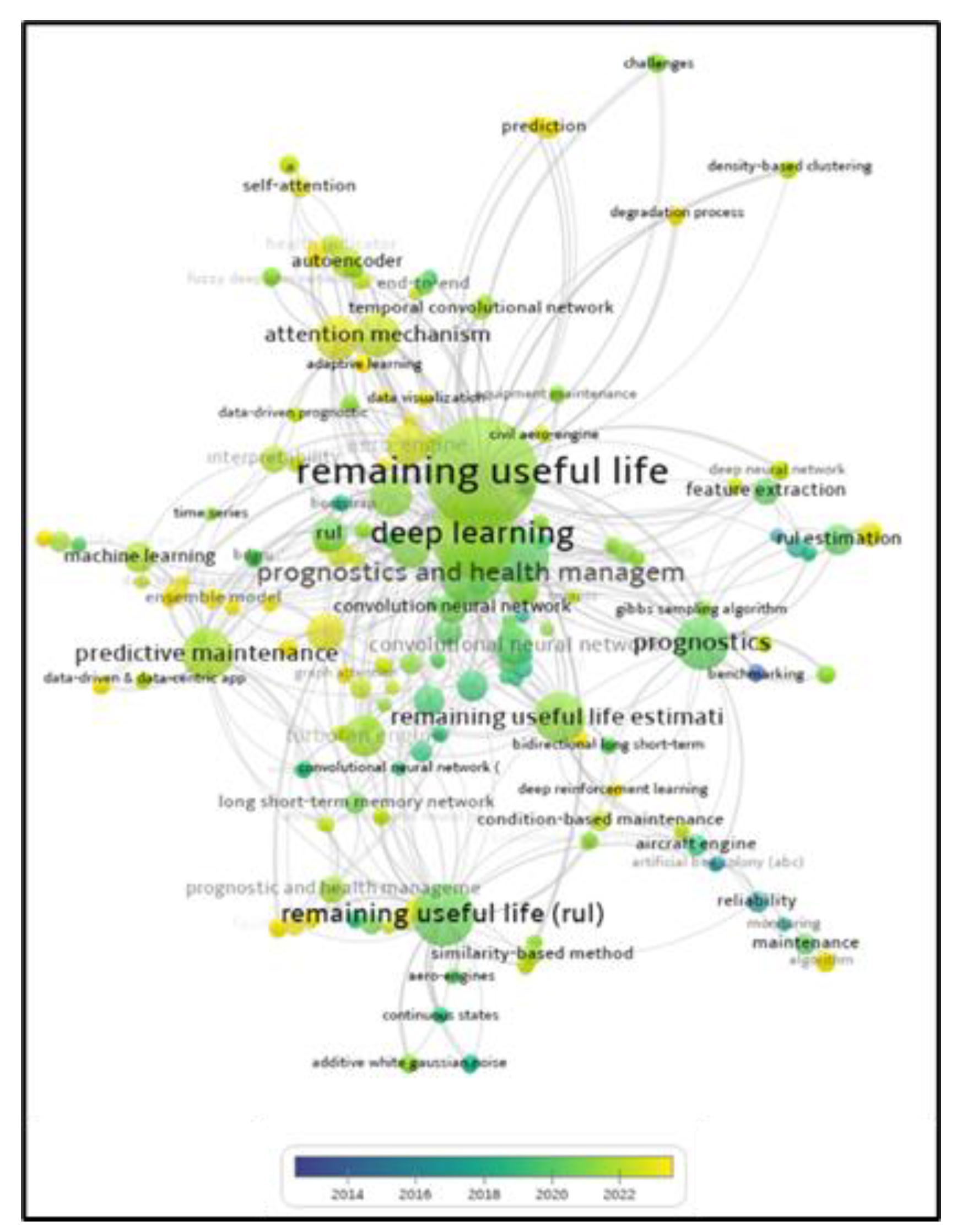
Figure 2.
Structure of ANN neurons.
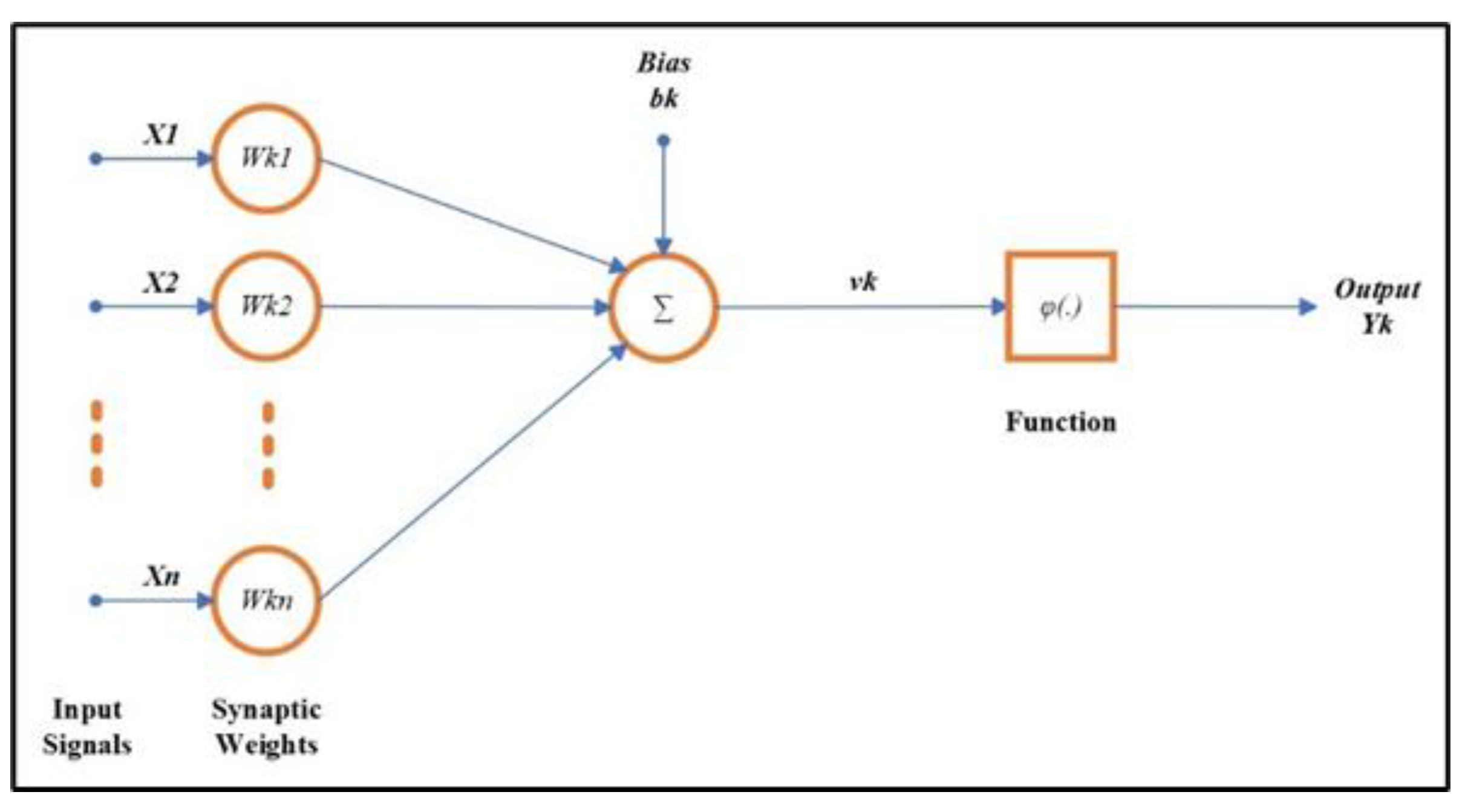
Figure 3.
Structure of ANN neurons.
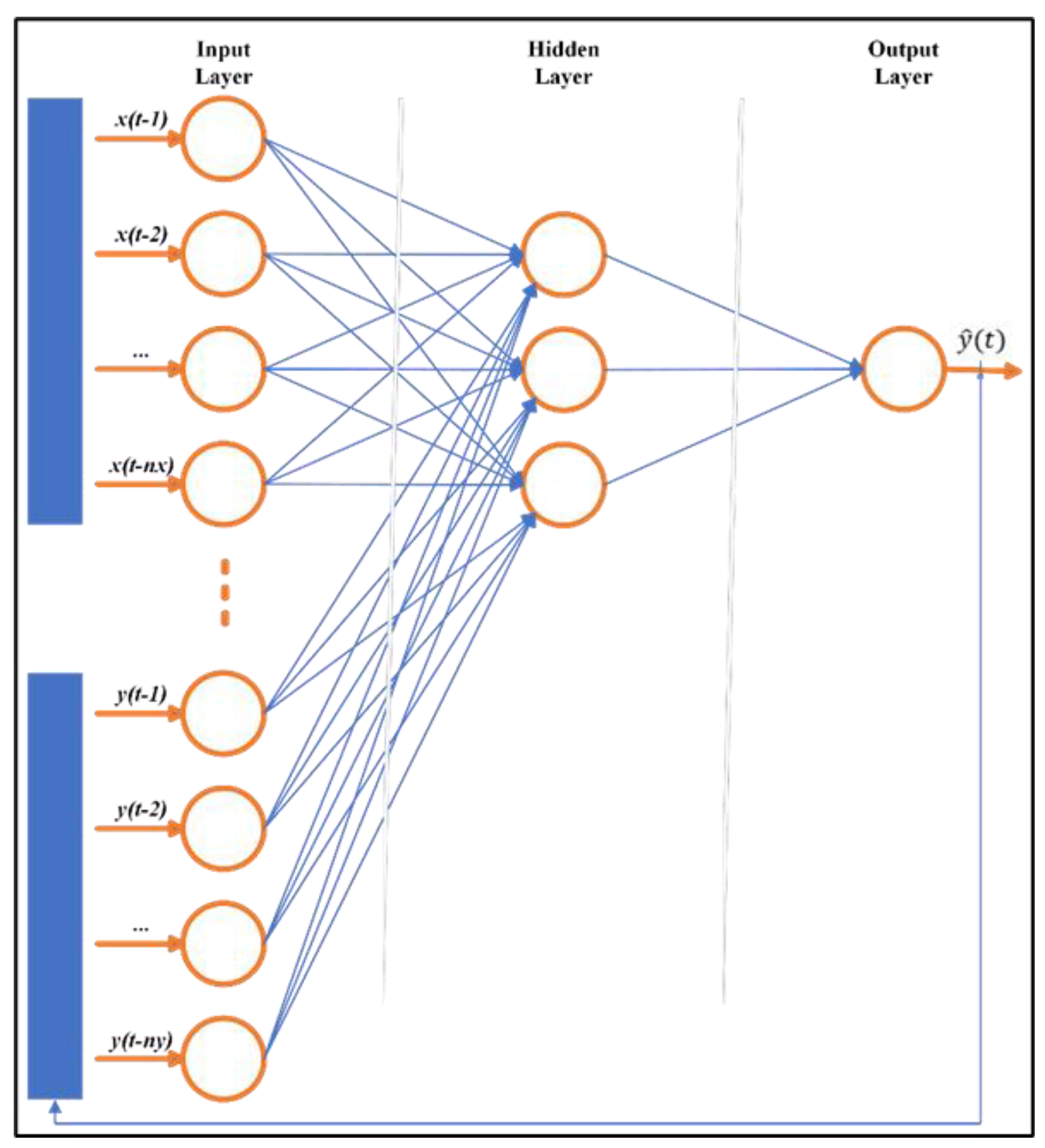
Figure 4.
a) Serries-parallel (open loop), b) Parallel (close loop) architecture in NARX model.
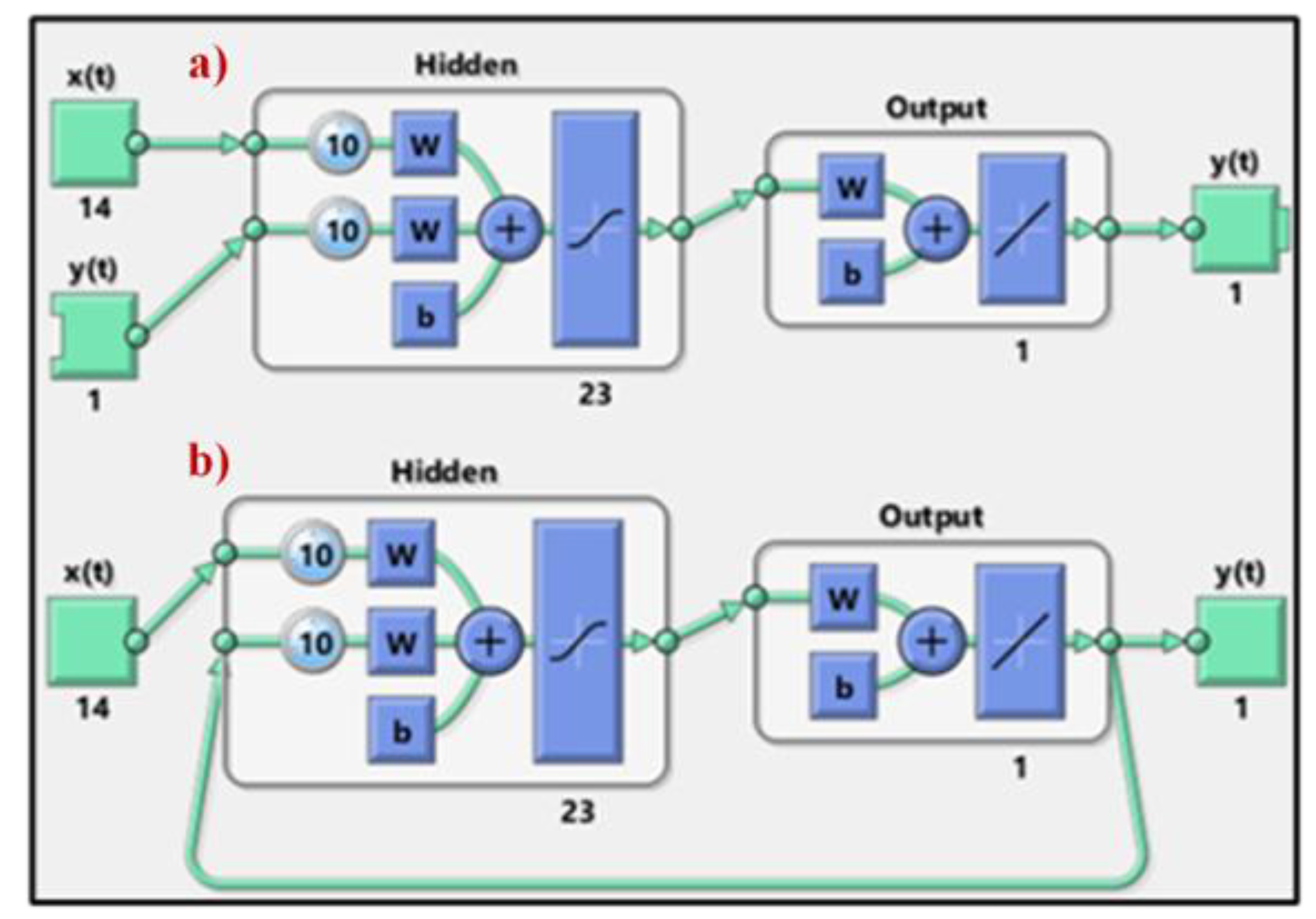
Figure 5.
Flowchart of the proposed methodology for RUL estimation.
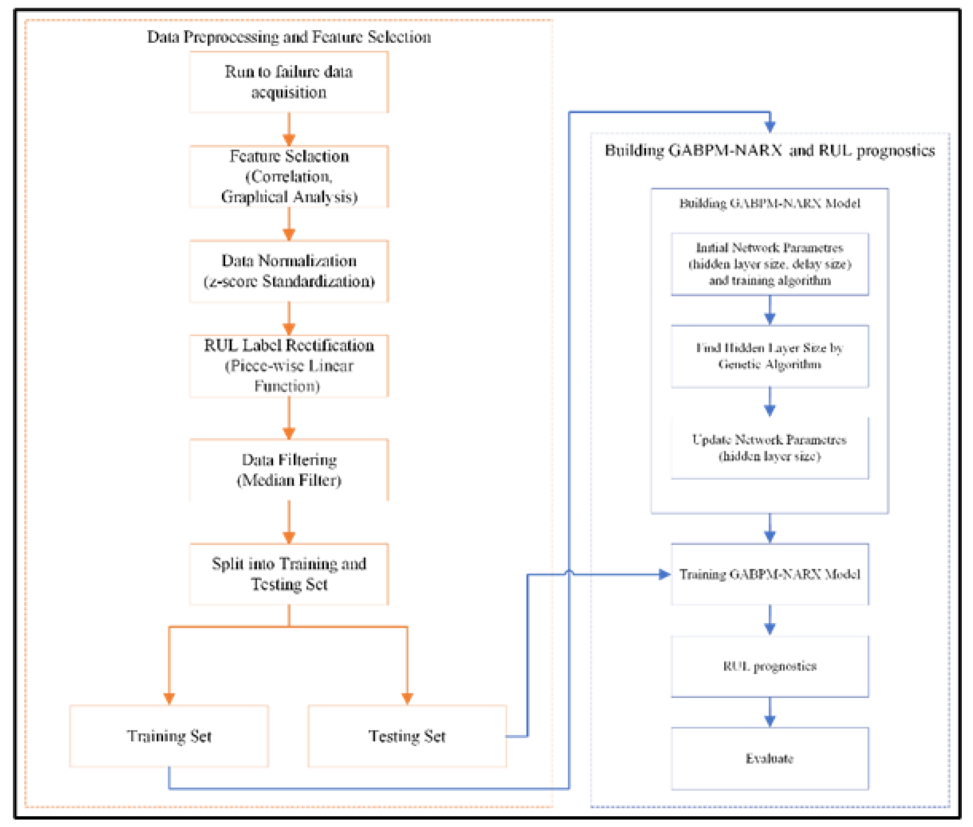
Figure 6.
Diagram of the turbofan simulation engine modules in C-MAPSS [25].
Figure 6.
Diagram of the turbofan simulation engine modules in C-MAPSS [25].
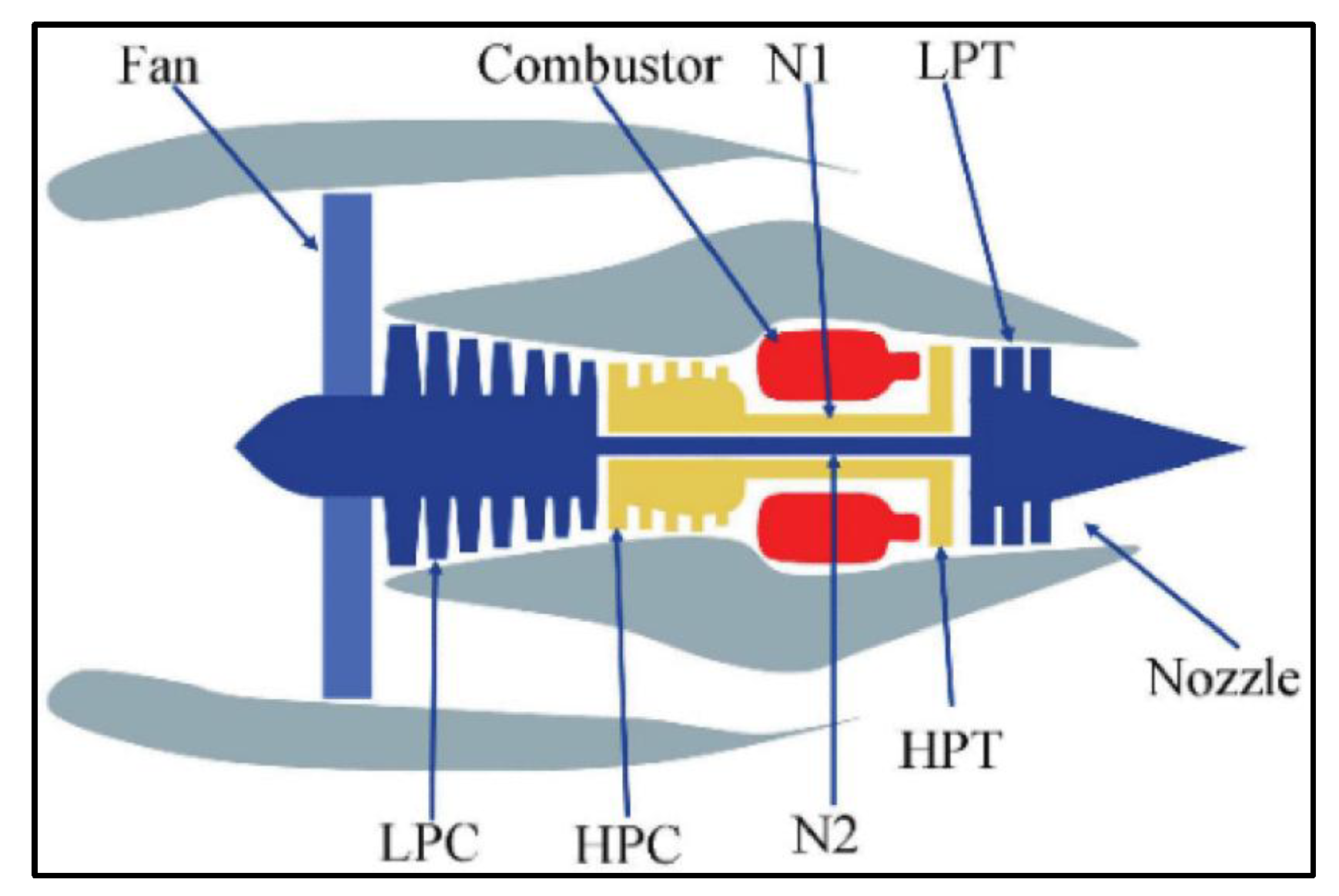
Figure 7.
Example times series plots of sensors.
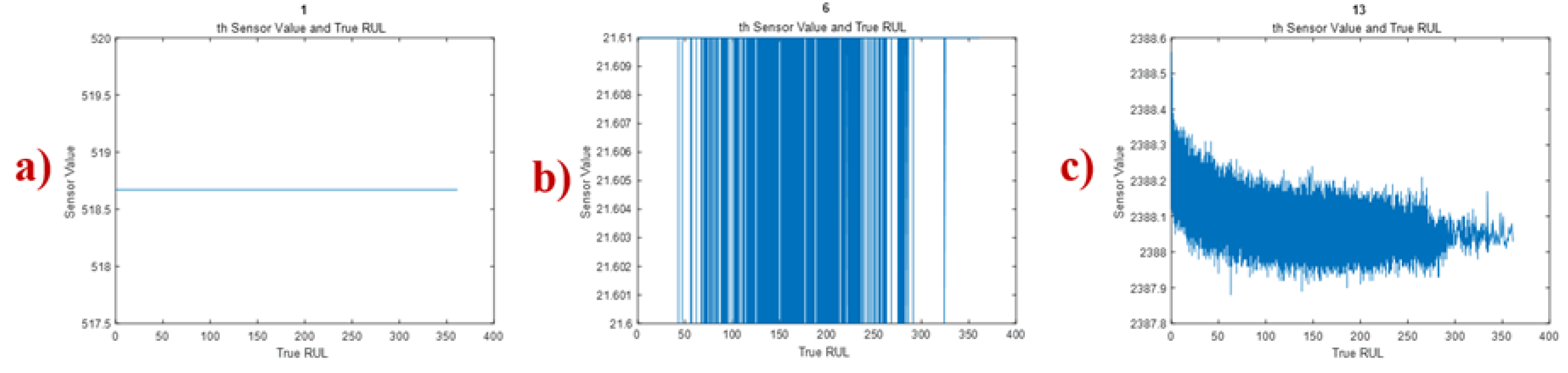
Figure 8.
Piece-wise RUL function of C-MAPSS dataset (piece-wise maximum RUL is 125-time cycles).
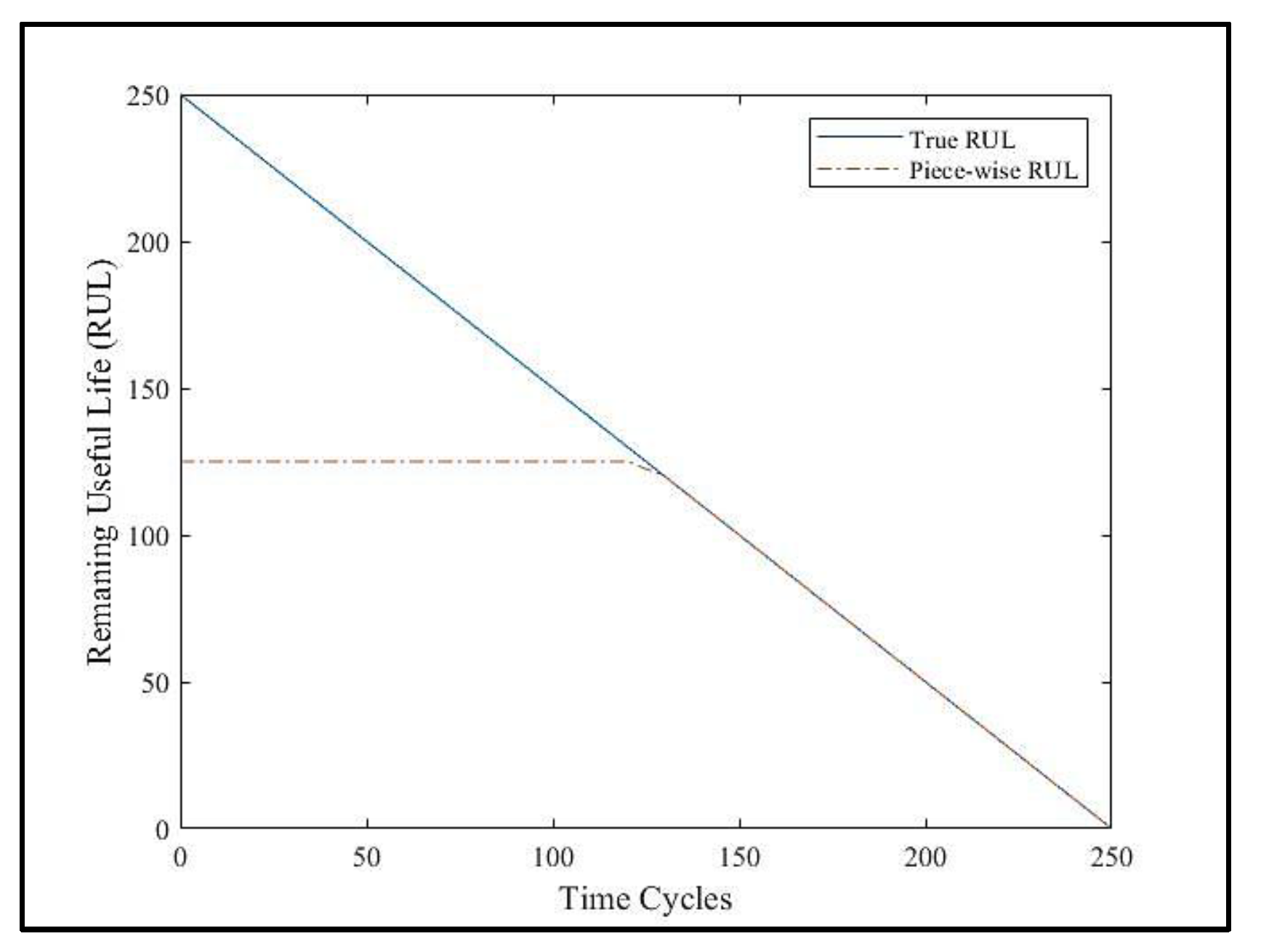
Figure 9.
Median filtering on different signals (Pratt, 1991).
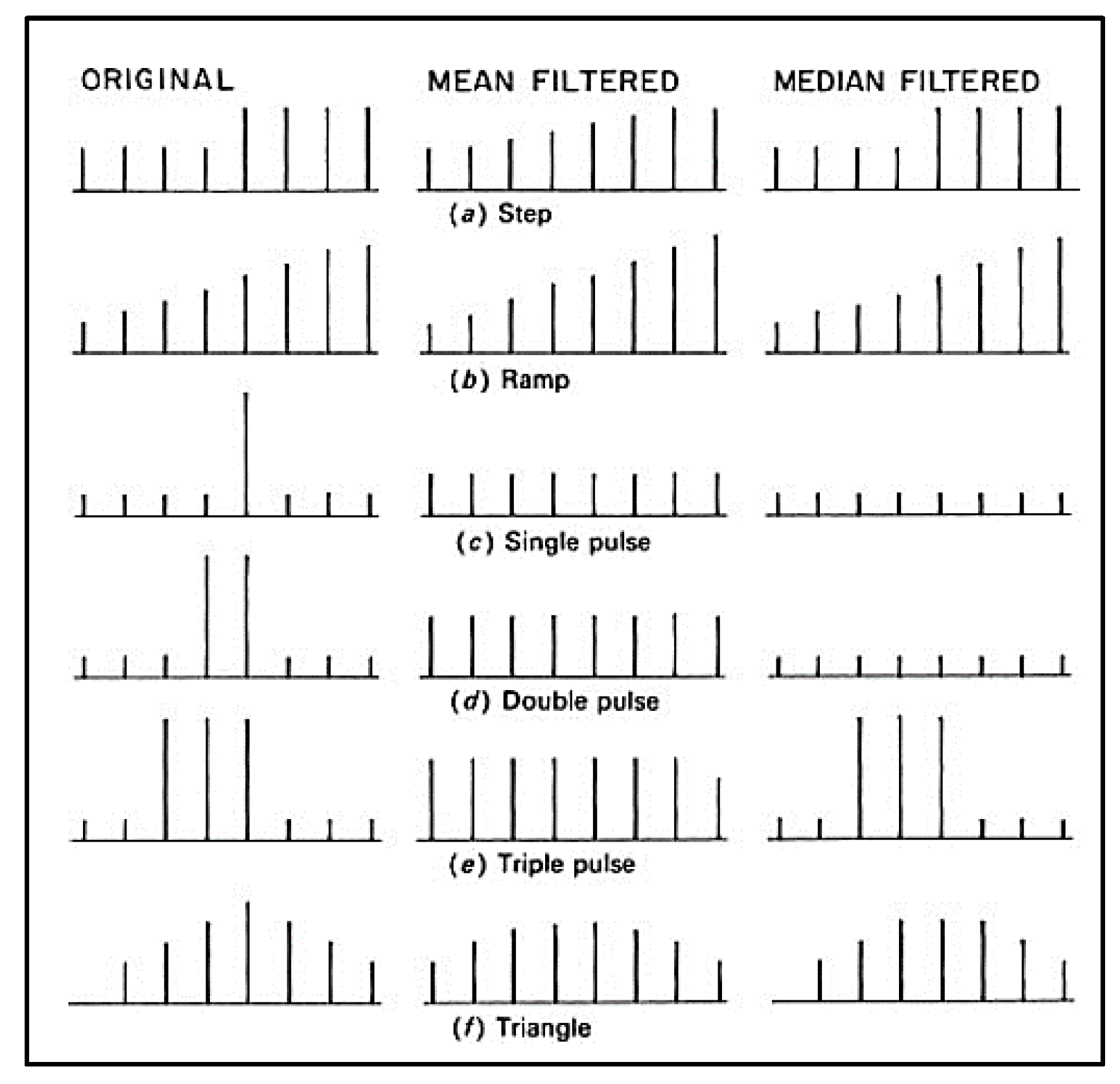
Figure 10.
Median filtering on C-MAPSS Sensor 3 and 15.
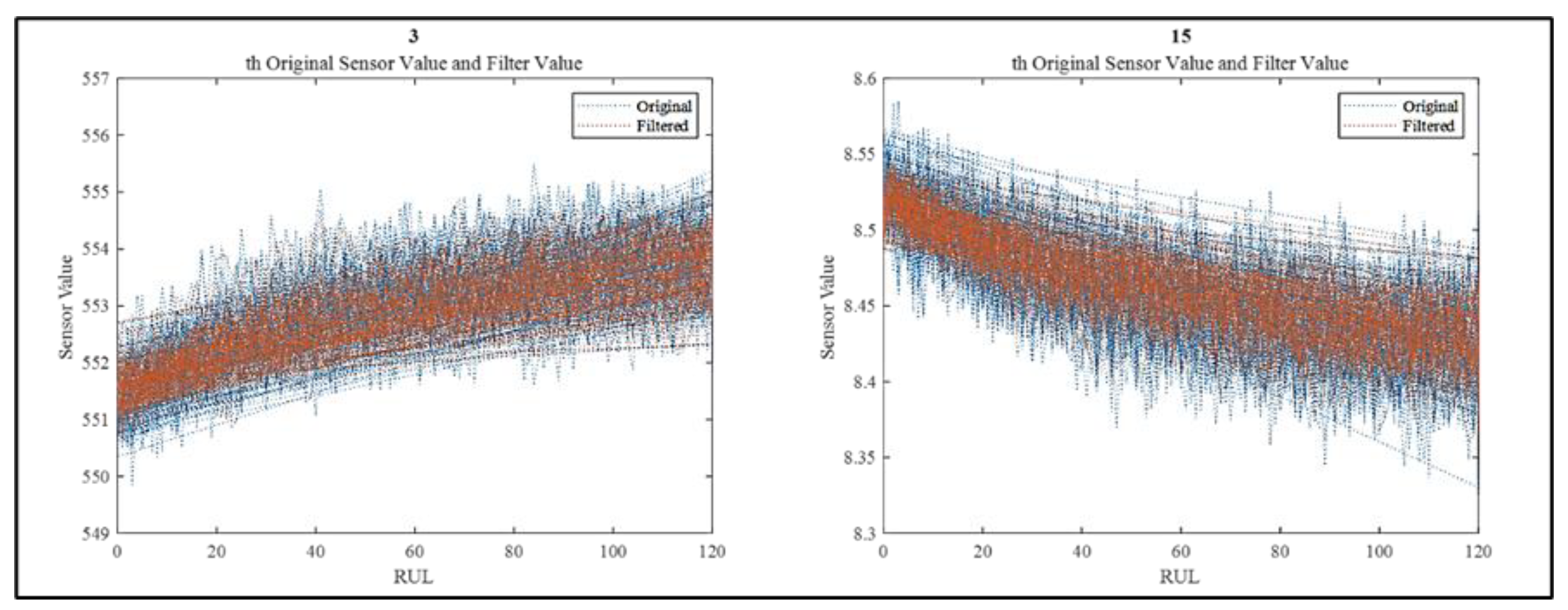
Figure 11.
Time series plot of the selected sensors.
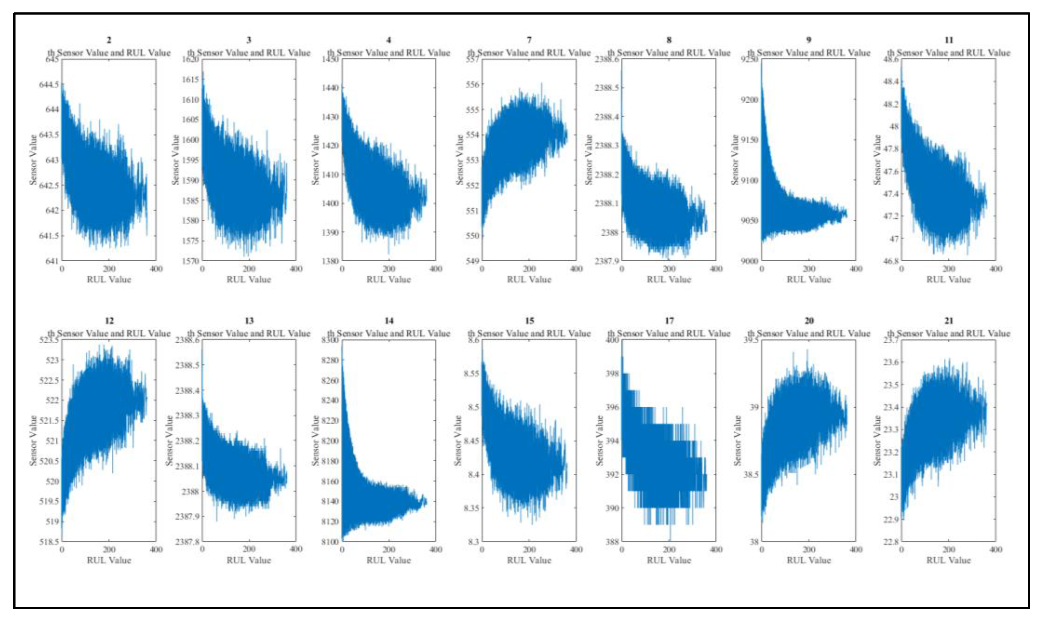
Figure 12.
Example of last similar 4 cycle-time window.
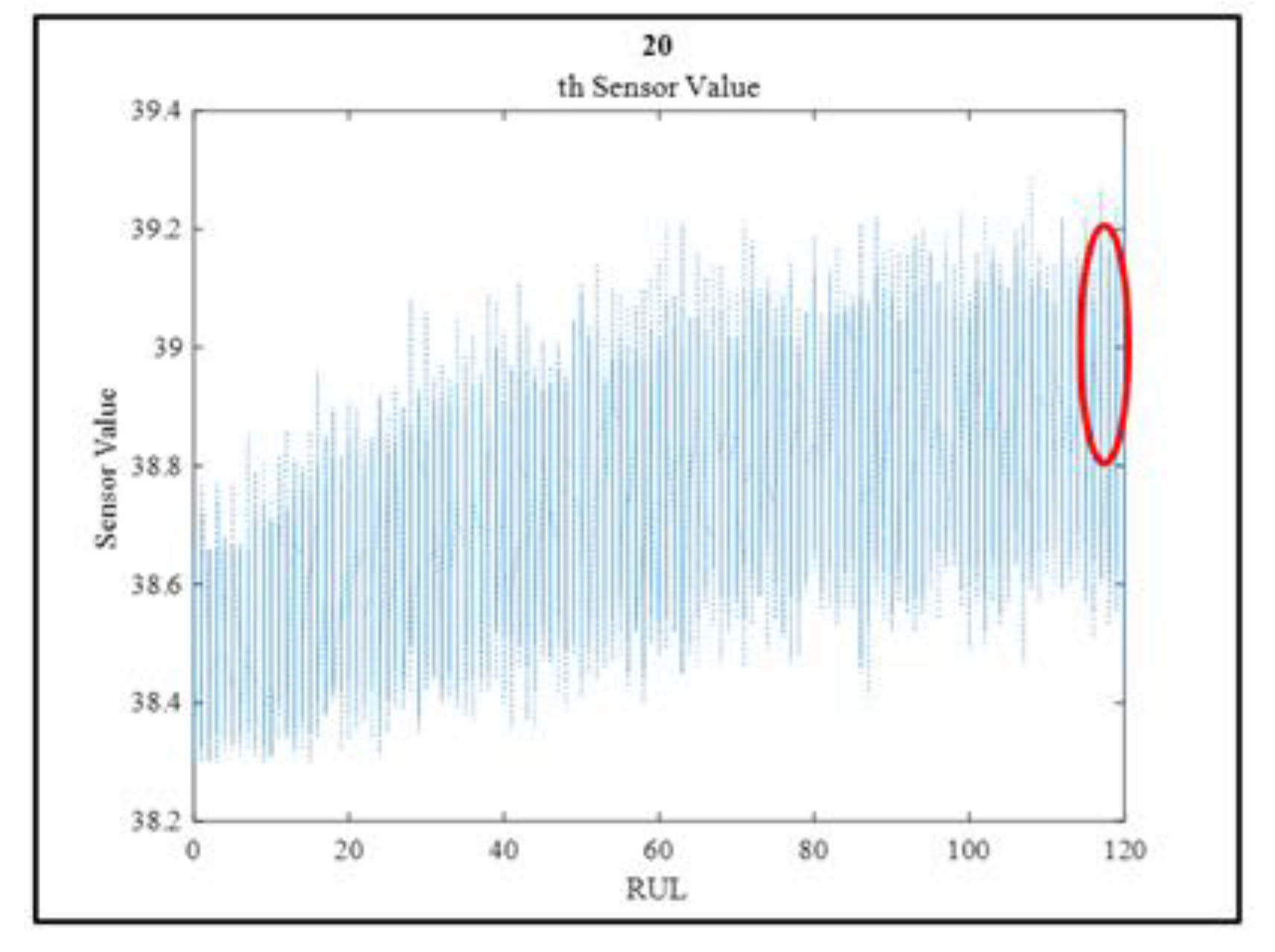
Figure 13.
Fitness function of the GA.
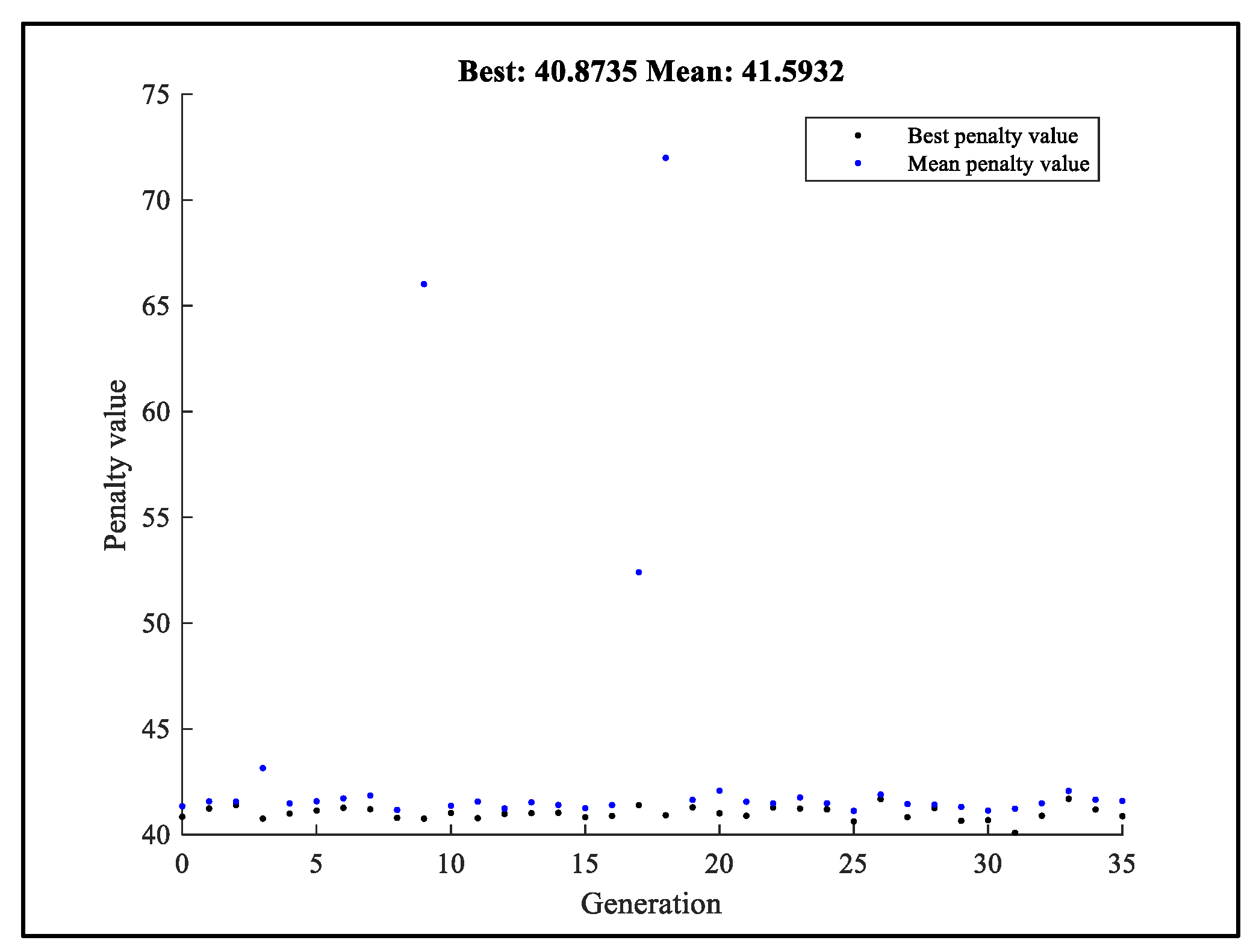
Figure 14.
Proposed GABPM-NARX model architecture for RUL estimation.
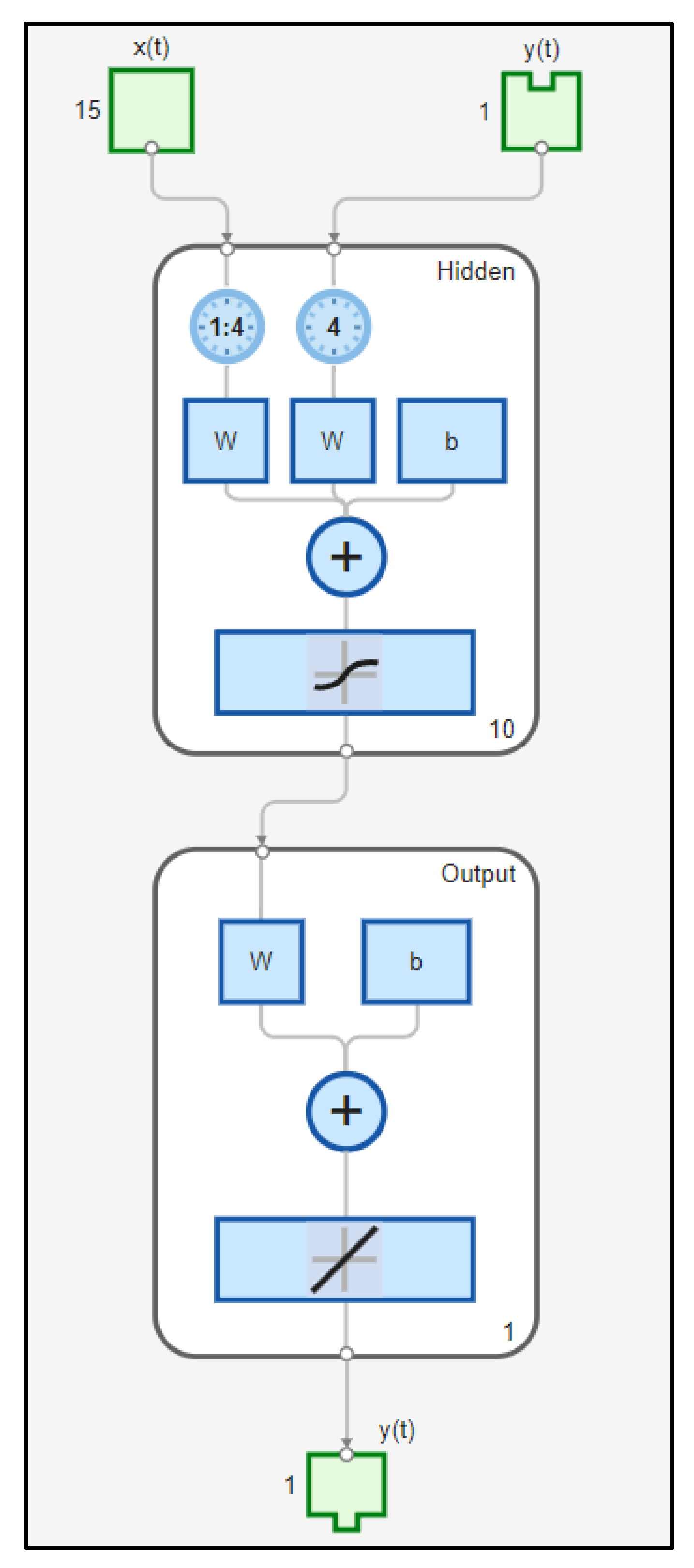
Figure 15.
GABPM-NARX model regression plot.
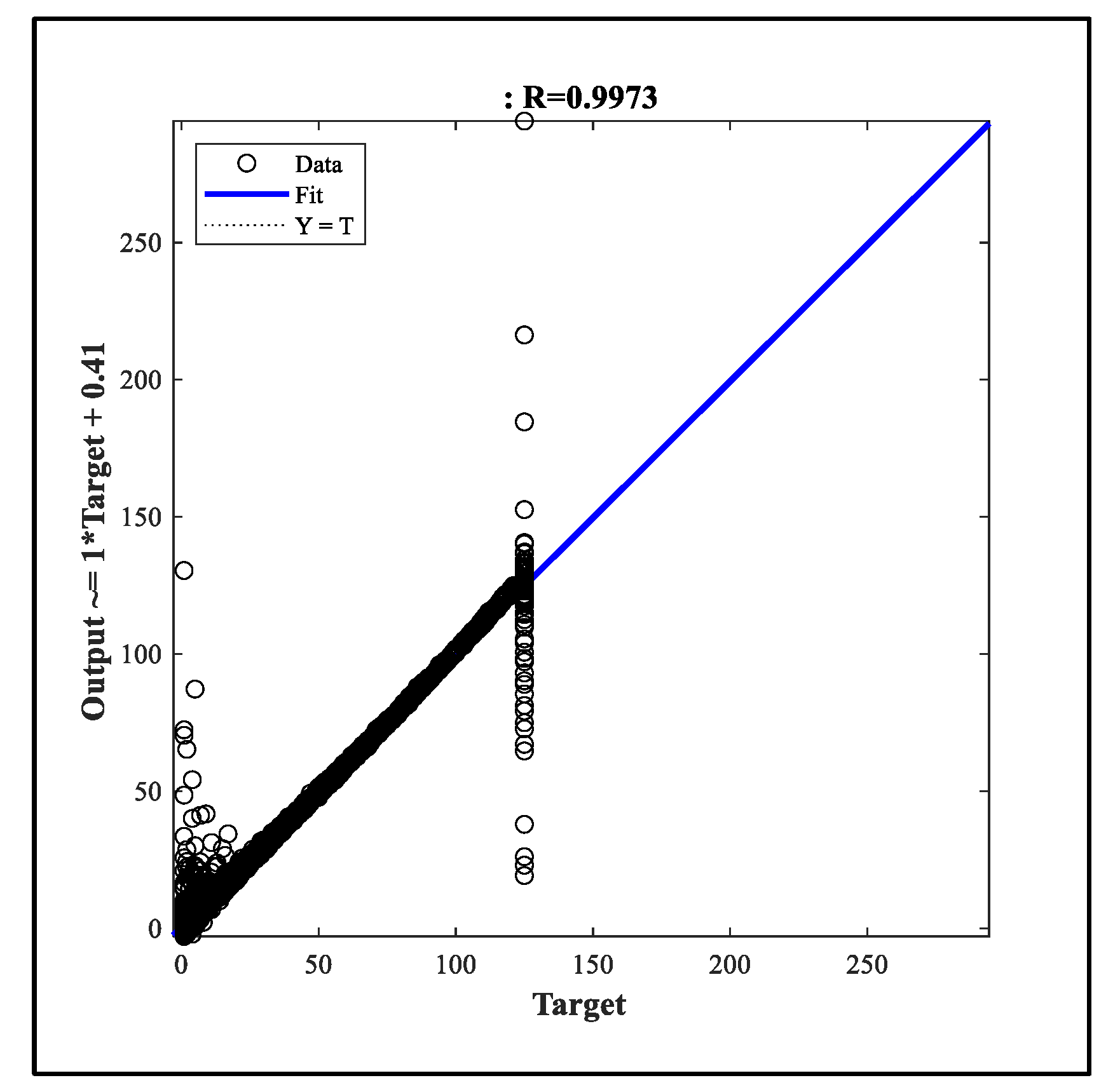
Figure 16.
GABPM-NARX model performance plot.
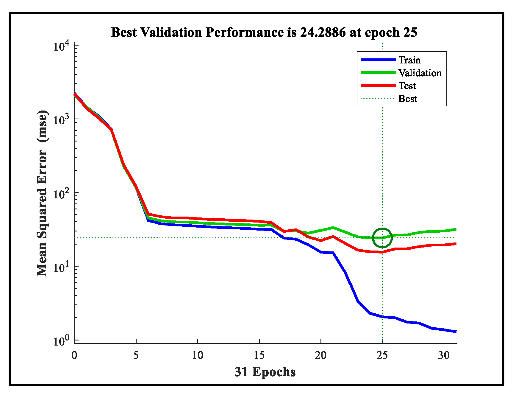
Figure 17.
GABPM-NARX model error histogram.
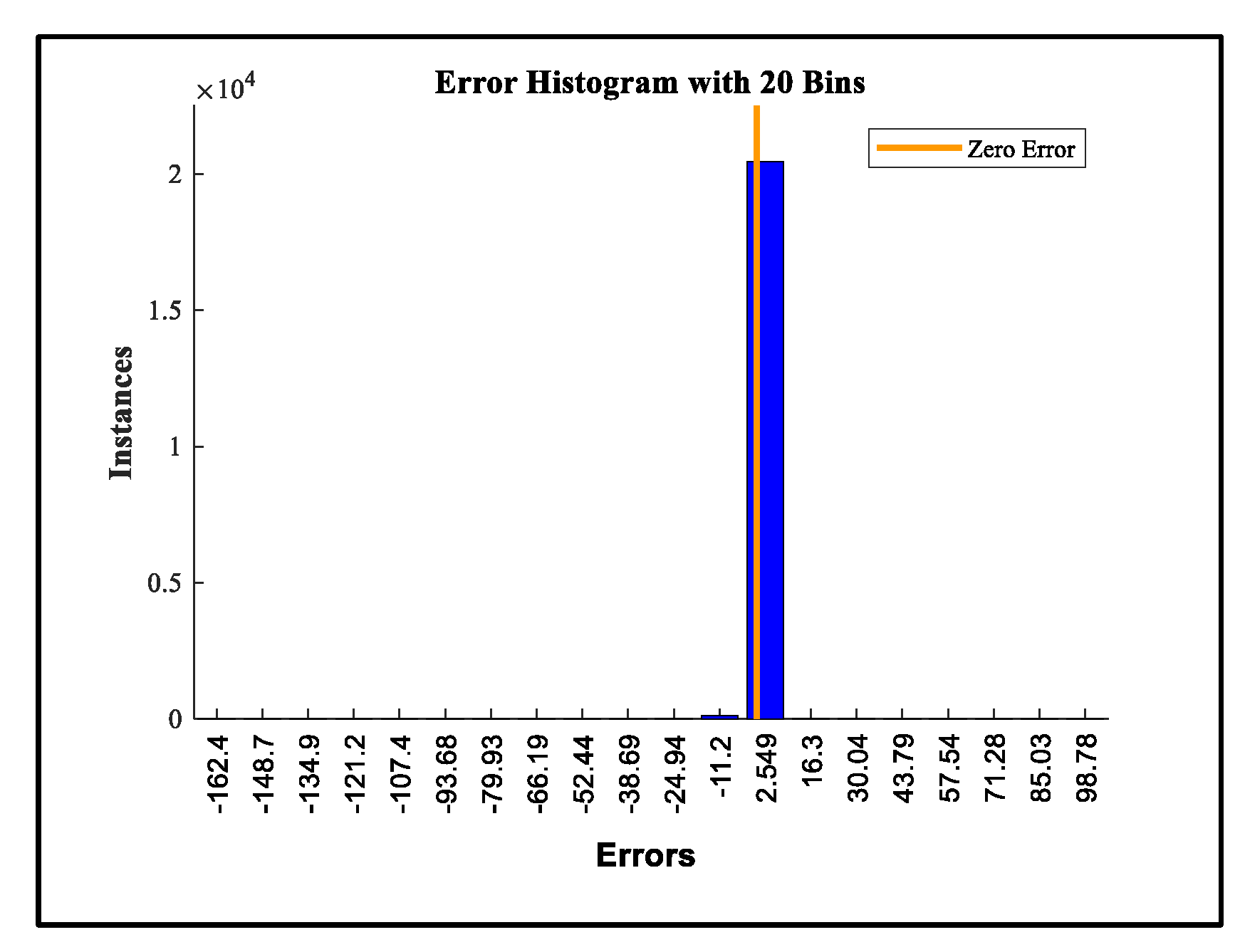
Figure 18.
GABPM-NARX autocorrelation function (ACF) histogram.
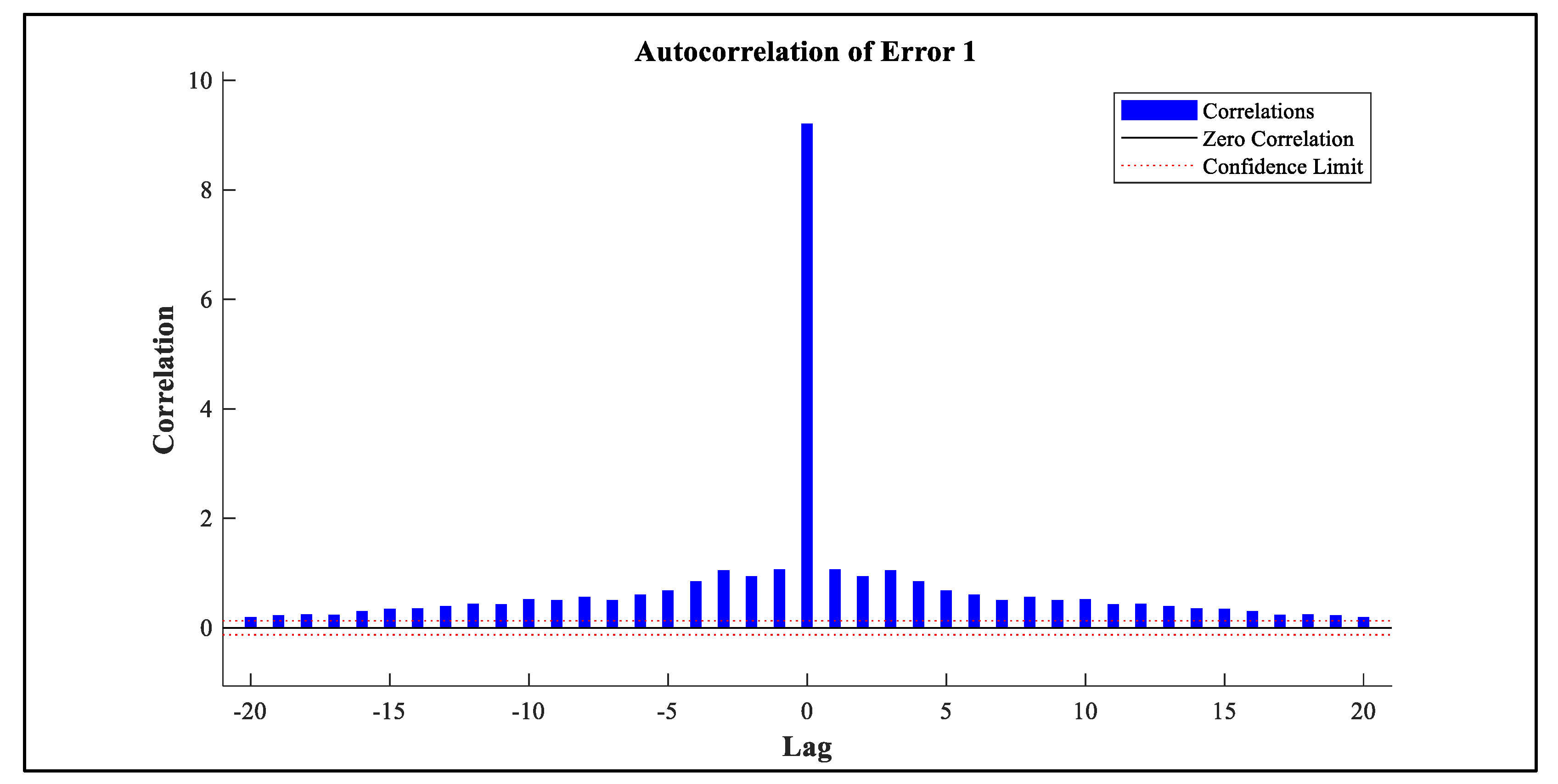
Figure 19.
GABPM-NARX Training Dynamics of Optimization Parameters Across Epochs.
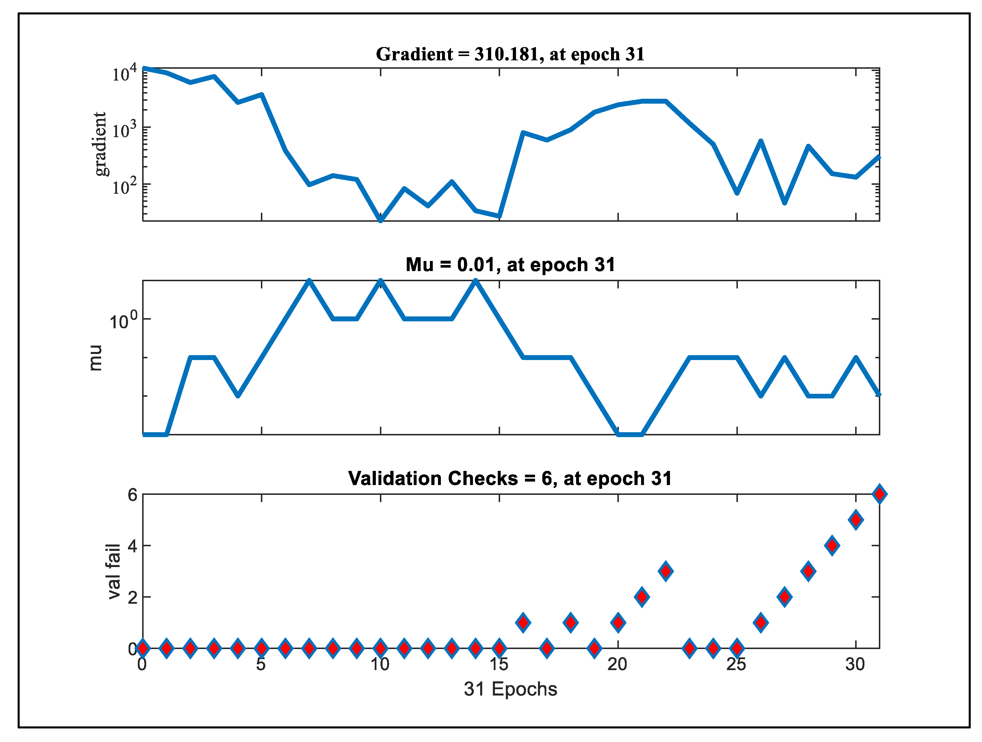
Figure 20.
Evaluation of Metric Structure Under Varying Error Conditions.
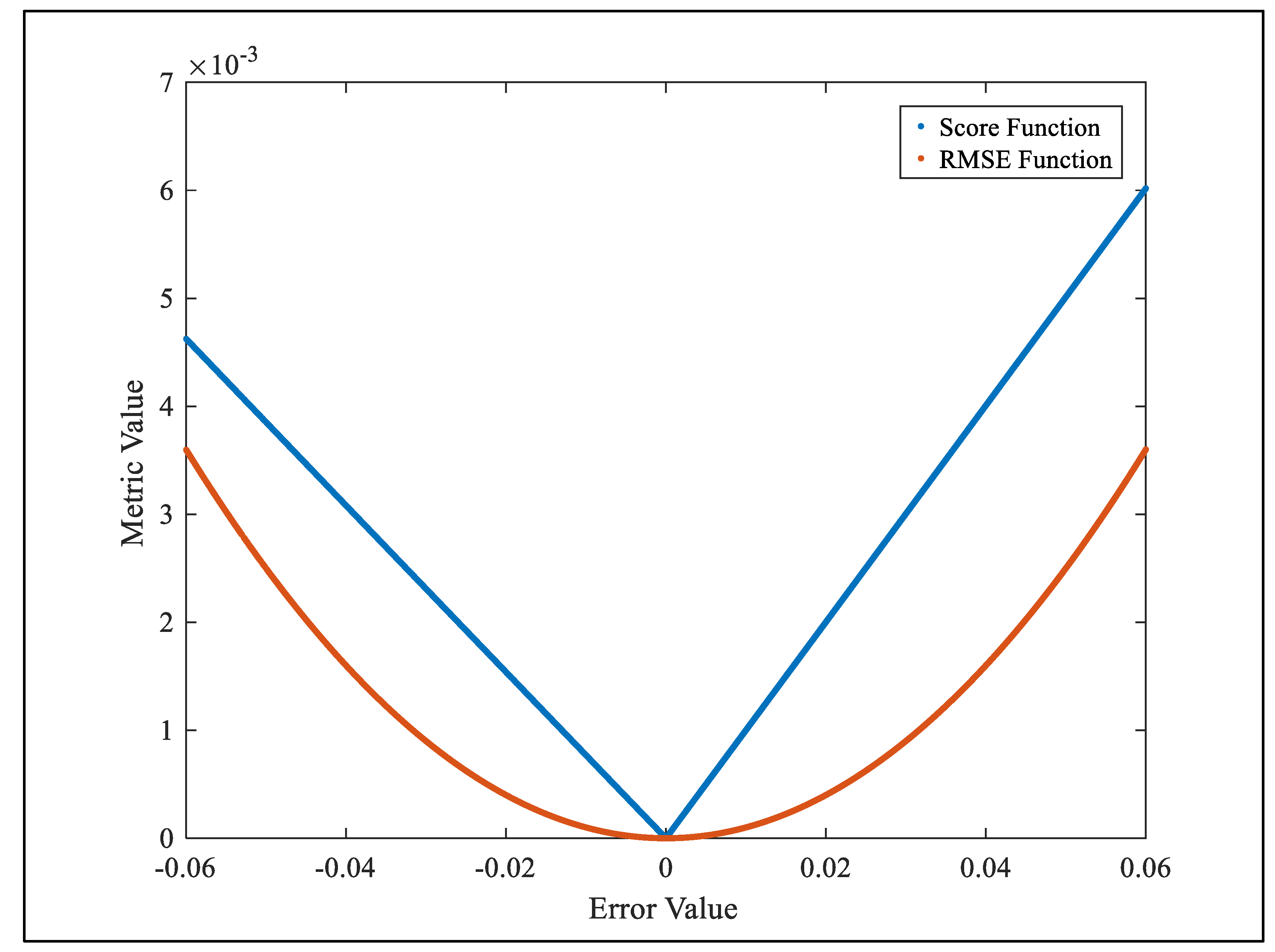
Figure 21.
Examples of RUL prediction results.
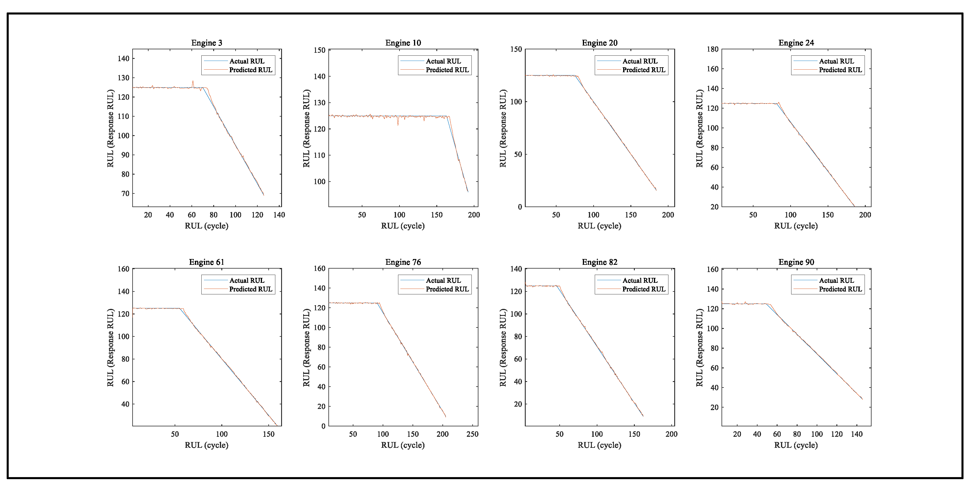

Table 1.
Literature summary on RUL estimation.
| References | Year | Framework | Data Preprocessing Steps | C-MAPSSFD001 | Contributions/Superiorities | |
|---|---|---|---|---|---|---|
| RMSE or MSE | Score | |||||
| [35] | 2017 | LSTM | Data normalization, RUL label rectification |
16.14; | 338 | Utilizing multiple layers of LSTM cells in combination with standard front layers to reveal hidden patterns in data. |
| [5] | 2020 | CNN, LSTM | Feature selection, Data normalization, RUL label rectification |
10.41 | N/A | Modelling a model by combining 1D CNN, LSTM, and Bi-LSTM algorithms. Intuitively identify critical features affecting RUL with Shapley additive Shapley explanation (SHAP). |
| [11] | 2020 | Multi Head CNN, LSTM | Feature selection, RUL label rectification |
12.19 | 259 | Recommending an approach that combines prediction error analysis (PEA) with the multi-head CNN-LSTM to improve prediction accuracy. |
| [15] | 2018 | BiLSTM | Feature selection, Data normalization, RUL label rectification |
13.65 | 295 | Proposing BiLSTM that can learn the dependencies of sensor data in both forward and backward directions. |
| [8] | 2019 | DAG CNN+LSTM | Feature selection, Data normalization, RUL label rectification |
11.96 | 229 | Proposing a directed acyclic graph (DAG) network combining a CNN and LSTM. Using a sliding time window (TW) to extract the data so that the model inputs have an equivalent short-term time series. |
| [7] | 2019 | LSTM+CNN | Feature selection, Data normalization, RUL label rectification |
16.16 | 303 | Using the threshold of variance detection method in feature selection. Coordinating the health index (HI) and selected variables into the input. Proposing a health index-based approach using LSTM+CNN. |
| [9] | 2020 | Novel Feature-Attention-Based End-to-End, CNN | Feature selection, Data normalization, RUL label rectification |
12.42 | 225 | Extracting distinguishing features of variables with a feature-attention mechanism. Forecasting with the recommended Feature-Attention-Based End-to-End approach. |
| [13] | 2021 | LSTM, 1- FCLCNN |
Feature selection, Data normalization, RUL label rectification |
11.17 | 204 | Two models to improve prediction by splitting data after data preprocessing; modeling as LSTM and 1-FCLCNN then combining models in terms of the spatiotemporal features and becoming one-dimensional CNN input. |
| [18] | 2021 | BLS, TCN | Feature selection, Data normalization, RUL label rectification |
12.08 | 243 | Combining two models into a broader learning system (BLS) and temporal convolutional network (TCN) for prediction. |
| [10] | 2021 | Bi-LSTM | Feature selection, RUL label rectification |
13.78 | 255 | Proposing the attention mechanism to give higher weight to important features by weighting the Bi-LSTM outputs, thus increasing the accuracy of the estimation. |
| [12] | 2022 | LSTM, Probabilistic deep learning methodology | Feature selection, Data normalization, Right padding, RUL label rectification |
149.5 (MSE) | 243.8 | Combining a probabilistic model (lognormal distribution) with a recurrent neural network model. Analytical formulation to assess the system's reliability and SRUL probability based on its structure. |
| [14] | 2016 | CNN | Data normalization, RUL label rectification |
18.44 | 1286.7 | On different time scales, the conspicuous patterns of the sensor signals are detected by the convolutional layer and the pooling layer. In this paper proposing deep learning for RUL estimation in prognostic problems, a new CNN-based architecture is proposed for estimating the RUL of the system from multivariate time series data. |
| [36] | 2017 | SVR | Feature selection, Data filtering, Extracting Trend Features |
N/A | 448.7 | Utilized in a health indicator that combines sensory data into a one-dimensional signal |
| [17] | 2021 | Classification + SVR, Gradient Boost, LSTM, CNN | Feature selection, Health stage classification |
16.89 | 732 | Predicting the classification of stages automatically at the stage level. |
| [16] | 2023 | Double deep CNN | Feature selection, Data filtering, RUL label rectification |
12.85 | 224 | The segment layer, information extraction layer, and information aggregation layer were created to learn the spatiotemporal fusion properties of the data. |
| [4] | 2023 | ARMA+GCN and GRU | Data filtering, Feature selection, Data standardization RUL label rectification |
11.60 | 191.05 | ARMAGCN and GRU-based designed approach is proposed for RUL estimation and the proposed physics-based loss function is expected to improve the accuracy of RUL estimation. |
| [20] | 2023 | CNN+GRU and self attention mechanisms | Data normalization, RUL label rectification |
11.91 | 227 | CNN and GRU as a hybrid network combined with a self-attention mechanism. |
| [37] | 2024 | LSTM- MLP | Data normalization, Feature Selection, Noise Reduction |
796.42 (MSE) | N/A | LSTM MLP: The LSTM model significantly outperforms the MLP in capturing temporal dependencies in engine degradation. LSTM maintains predictive performance across different engine units, demonstrating scalability. - The study highlights how LSTM-based RUL prediction can shift maintenance strategies from reactive to proactive, reducing downtime and costs. |
| [38] | 2024 | Multi-IFFGRU | Feature Selection, Normalization, Sliding Window Segmentation, Feature Filtering |
9.82 | 98.17 | The multi-branch structure ensures independent feature extraction for each sensor. - The Inception module enhances spatial feature extraction, addressing CNN limitations. Assigns importance weights to extracted features, improving prediction accuracy. Extensive ablation experiments confirm the necessity of each module. Despite improvements, the model maintains reasonable computational costs. |
| [39] | 2025 | Fusion-based dual-task architecture | Normalization, Feature Selection, Sliding Window Segmentation, RUL Label Reconstruction |
5.67 | 15.95 | - The integration of DM identification and RUL prediction improves accuracy. - ResNet extracts single-flight features, while LSTM captures temporal dependencies. The model refines RUL predictions using degradation information. The model maintains high accuracy across different degradation modes. |
| Proposed GABPM-NARX model | 2025 | NARX with meta-heuristic support | Feature selection, Data normalization, Data filtering, RUL label rectification |
3.0331 | 12.5216 | Utilizing effective data preprocessing steps allows the prediction model to obtain more accurate predictions of RUL. Solving the non-linear mathematical model written to increase the prediction success to determine the parameters in the NARX network with the meta-heuristic method, thus modeling with the NARX in a way that increases the prediction accuracy. |
Table 2.
C-MAPSS dataset.
| Dataset | FD001 | FD002 | FD003 | FD004 |
|---|---|---|---|---|
| Number of engines/units | 100 | 260 | 100 | 249 |
| Number of training samples | 20631 | 53579 | 24270 | 61249 |
| Number of test samples | 100 | 259 | 100 | 248 |
| Operating conditions | 1 | 6 | 1 | 6 |
| Fault conditions | 1 | 1 | 2 | 2 |
Table 3.
Data description of C-MAPSS sensors.
| Sensors | Symbol | Particulars | Units |
|---|---|---|---|
| Sensor 1 | T2 | Total temperature at fan inlet | °R |
| Sensor 2 | T24 | Total temperature at LPC outlet | °R |
| Sensor 3 | T30 | Total temperature at HPC outlet | °R |
| Sensor 4 | T50 | Total temperature at LPT outlet | °R |
| Sensor 5 | P2 | Pressure at fan inlet | psia |
| Sensor 6 | P15 | Total pressure in bypass-duct | psia |
| Sensor 7 | P30 | Total pressure at HPC outlet | psia |
| Sensor 8 | Nf | Physical fan speed | rpm |
| Sensor 9 | Nc | Physical core speed | rpm |
| Sensor 10 | epr | Engine pressure ratio | … |
| Sensor 11 | Ps30 | Static pressure at HPC outlet | psia |
| Sensor 12 | Phi | Ratio of fuel flow to Ps30 | pps/psi |
| Sensor 13 | NRf | Corrected fan speed | rpm |
| Sensor 14 | NRc | Corrected core speed | rpm |
| Sensor 15 | BPR | Bypass ratio | … |
| Sensor 16 | farB | Burner fuel-air ratio | … |
| Sensor 17 | htBleed | Bleed enthalpy | … |
| Sensor 18 | Nf_dmd | Demanded fan speed | Rpm |
| Sensor 19 | PCNfR_dmd | Demanded corrected fan speed | Rpm |
| Sensor 20 | W31 | HPT coolant bleed | lbm/s |
| Sensor 21 | W32 | LPT coolant bleed | lbm/s |
1 Tables may have a footer.
Table 4.
Pearson correlation coefficients (selected sensors are given in bold characters).
| Sensors | RUL |
|---|---|
| Sensor 1 | - |
| Sensor 2 | -0.68 |
| Sensor 3 | -0.66 |
| Sensor 4 | -0.76 |
| Sensor 5 | - |
| Sensor 6 | -0.11 |
| Sensor 7 | 0.74 |
| Sense 8 | -0.63 |
| Sensor 9 | -0.47 |
| Sensor 10 | - |
| Sensor 11 | -0.78 |
| Sensor 12 | 0.75 |
| Sensor 13 | -0.63 |
| Sensor 14 | -0.37 |
| Sensor 15 | -0.72 |
| Sensor 16 | - |
| Sensor 17 | -0.68 |
| Sensor 18 | - |
| Sensor 19 | - |
| Sensor 20 | 0.71 |
| Sensor 21 | 0.71 |
Table 5.
GA parameters and mathematical models.
| Genetic algorithm | |
|---|---|
| Decision variable |
delaySize hiddenLayerSize |
| Fitness function (minimize) | RMSE_sample_NARX_fitness_func |
| Constraints |
delaySize>=0 hiddenLayerSize>=1 |
| Population size | 5 |
| Generations | 35 |
| Elite count | 3 |
Disclaimer/Publisher’s Note: The statements, opinions and data contained in all publications are solely those of the individual author(s) and contributor(s) and not of MDPI and/or the editor(s). MDPI and/or the editor(s) disclaim responsibility for any injury to people or property resulting from any ideas, methods, instructions or products referred to in the content. |
© 2025 by the authors. Licensee MDPI, Basel, Switzerland. This article is an open access article distributed under the terms and conditions of the Creative Commons Attribution (CC BY) license (http://creativecommons.org/licenses/by/4.0/).
Copyright: This open access article is published under a Creative Commons CC BY 4.0 license, which permit the free download, distribution, and reuse, provided that the author and preprint are cited in any reuse.


