Submitted:
29 June 2025
Posted:
30 June 2025
You are already at the latest version
Abstract
In traditional aggregate grading analysis, sieving is the most common technique, which separates samples using sieves with different mesh sizes. However, this approach is unscalable and environmentally unfriendly. In this study, we propose a deep grading for aggregate pre-screening based on the Segment Anything Model (SAM) and the Kolmogorov-Arnold Network (KAN). This method first utilizes SAM for automatic image segmentation, followed by minor manual interactive correction to modify the segmentation contour. Subsequently, the ellipse fitting is performed to calculate four geometric quantities (minor axis, major axis, area, perimeter) of each aggregate. Lastly, KAN is employed to predict to which particle size range an aggregate belongs and the volume from these four geometric quantities, thereby forming a compliant or non-compliant gradation curve for a cluster. Experimental results demonstrate that just with 2D images, deep grading can achieve >80% accuracy in compliance prediction for aggregate clusters, which reflects that deep grading is qualified as a pre-screening method.
Keywords:
Aggregate Gradation
; deep learning
; Image Segmentation
; KAN
1. Introduction
Aggregate grading [1] is a critical step in the construction industry, significantly influencing the quality and performance of concrete and asphalt, including workability, strength, and durability. Properly graded aggregates can minimize voids and ensure a dense and robust mix, thereby preventing cracking and enhancing the durability of concrete. Additionally, a well-graded mix requires less water to achieve the desired consistency, thereby reducing the risk of segregation during the pouring process.
Currently, the aggregate grading mainly relies on mechanical equipment and manual assistance, which consists of two steps: First, with vibrating screens or trommel screens, aggregates are separated into different sizes. Then, aggregates are sorted into stockpiles according to the size, and the size distributions will be tallied. Hereafter, we call for brevity this kind of aggregate grading method traditional. Though traditional aggregate grading has served the construction industry for decades, it has several intrinsic disadvantages that cannot be easily addressed. 1) Capital investment is high: The purchase and maintenance of heavy machinery such as screens and washing plants involves a substantial capital investment. Moreover, expenses for fuel, maintenance, and staffing can add up to the overall project budget. 2) Due to the limited size and efficiency of the machinery, it struggles to handle large-scale grading tasks in diverse scenarios. 3) The screening process generates significant noise and dust, requiring additional actions for dust control and environmental protection. To solve these problems, some researchers attempted to leverage the image segmentation algorithm for grading [2,3]. However, the traditional image processing algorithm has restricted segmentation ability to characterize the geometry of aggregates, i.e., mistakenly regarding some aggregates as background, failing to address some aggregates of non-convex shape, etc.
Artificial intelligence is reshaping the industry towards the significantly enhanced efficiency and productivity [4,5,6]. In this context, we explore the feasibility of applying deep learning algorithms to aggregate grading, which we hereafter refer to as “deep grading." As an initial step, we propose using deep grading to prescreen aggregates. The core task of grading involves determining whether aggregates can pass through a sieve of a specific size after sufficient vibration. Our central idea is that the state-of-the-art image segmentation algorithms can characterize the shape of aggregates directly and accurately. Then, based on these segmentation, we can compute various metrics to plot grading curves, thereby eliminating the need for machinery and its associated operations. Deep grading not only improves efficiency but also accurately identifies and stores the particle shape and size. Specifically, our proposed deep grading methodology consists of three steps:
i) Image segmentation. We first collect the image of aggregates and then use an advanced image segmentation algorithm to extract a two-dimensional (2D) profile of each aggregate. In recent years, significant advancements have been made in the field of image segmentation, particularly with the emergence of the Segment Anything Model (SAM, [7,8]). SAM is trained on a large and diverse dataset with 1B masks and 10,000,000 images. These images are annotated with segmentation masks that delineate object boundaries, which provide the model with the necessary information to learn how to identify and segment objects in images. Moreover, SAM utilizes a transformer-based architecture, which is effective in handling the complexities of image semantics. The powerful architecture and massive data enable the model to achieve high accuracy and generalization in identifying and segmenting objects in diverse images. Our proposed deep grading employs SAM for the automated segmentation of aggregate images to get 2D profiles of aggregates.
ii) Geometric information extraction. As Figure 1 shows, given the 2D profile of an aggregate, we use the elliptical fitting to construct the smallest ellipse to cover the aggregate. Then, four geometric quantities (short ax, long ax, area, perimeter) will be computed based on this ellipse, resulting in a feature vector of .
iii) Pre-screening. We construct a classifier to judge whether the given aggregates are qualified or not. Recently, the Kolmogorov-Arnold Network (KAN, [9]) represents a significant advancement in the basic deep learning architecture. This network draws its inspiration from the renowned Kolmogorov-Arnold representation theorem, which posits that any continuous multivariate function can be expressed as a sum of continuous univariate functions combined through addition. Specifically, Kolmogorov’s theorem indicates that for any , a continuous function can be decomposed as follows:
where and are continuous univariate functions. This theorem effectively transforms a d-dimensional multivariate function into a composition of univariate functions. Extensive experiments have shown that KAN has a strong representation ability. Therefore, we cast KAN as the classifier for predicting the category of each aggregate and the volume from the aforementioned four geometric quantities. To the best of our knowledge, it is the first time that KAN is applied in the field of civil engineering. Lastly, we carefully prepare the dataset, we show via systematic and comprehensive experiments that deep grading can deliver an over 80% prediction rate. This means that deep grading can serve as an effective pre-screening method.
As a paradigm innovation, deep grading has the potential of completely solving the aforementioned intrinsic issues in traditional aggregate grading. As Table 1 shows, first, the core of deep grading is the algorithm, which is easily enabled by combining simple apparatus like a camera and a computer. Thus, deep grading is cheaper than traditional grading. Second, deep grading is highly scalable, it is easy to quickly collect geometric information of a great amount of aggregates after the calibration. Third, deep grading is environmentally friendly, as no noise and dust are generated. Though not super precise, it is already satisfactory as a pre-screening method. In summary, our contributions are threefold:
- This study proposes the deep grading method for aggregate gradation, which is a paradigm shift. Compared to traditional aggregate grading, deep aggregate grading is cheaper, more scalable, and more environmentally friendly. This research pushes the application boundary of deep learning technologies in the sector of civil engineering. Furthermore, it holds potential for extension to all industries involving particle size distribution detection, such as pharmaceuticals, food processing, and mining.
- As the initial step, we introduce the SAM and KAN as the components of deep grading. To the best of our knowledge, this is the first time that SAM and KAN are used in the problem of aggregate grading analysis.
- Comprehensive and systematic experiments show that deep grading is competent for aggregate prescreening. Our research paves the way for the future large-scale application of deep grading in civil engineering. In addition, it is worth noting that our datasets are well-curated, which may be of independent interest. We open-source our dataset at Zenodo (https://zenodo.org/uploads/15661205) for practitioners’ free access and testing.
2. Related Work
Development of Aggregate Grading Methods. Grading [1] describes the mass distribution state of particles within various size ranges in granular materials, characterized by the mass percentage passing through each sieve aperture. Grading theory defines the ideal state of continuous gradation, where the gradation curve should conform to a specific distribution, such as the parabolic distribution, when the particle packing achieves the maximum density. Based on the particle size distribution characteristics, grading can be classified into three main types: continuous grading (with a continuous particle size distribution), gap grading (lacking specific intermediate particle sizes), and open grading (coarse particles form a skeletal structure). These types exhibit distinct mechanical and physical properties, leading to different performance characteristics [10,11]. Accurate grading is a critical aspect of engineering production. Sieving is commonly employed for gradation analysis, involving the physical separation and classification of materials based on the particle size. Mechanical sieving passes aggregates through a series of progressively finer screens. Each screen captures particles larger than a specified size, thereby separating them from finer materials. This method has been widely used in civil and material engineering for decades [12]. However, they require manual handling, leading to cumbersome and time-consuming procedures. Furthermore, when processing a great amount of samples or pursuing precise gradation, the accuracy is not guaranteed, and the scalability is limited, which fails them as modern digital and intelligent detection technologies.
Later, with breakthroughs in image processing technologies, aggregate analysis methods employing image processing techniques are developed towards faster and more accurate grading [13]. Unlike traditional gradation calculation methods that rely on cumulative weight percentages from physical sieving, digital aggregate analysis uses image parameters as independent variables. Image processing algorithms are employed to extract particle characteristics such as equivalent diameter and projected area, which are then used to compute gradation distribution. A gradation model is established by mapping geometric features to sieve sizes. Due to the limited capability of traditional image processing algorithm, the primary limitation of digital aggregate analysis lies in its inability to fully characterize the morphological information of aggregates in a single capture. The analysis is sensitive to imaging angles, which may introduce errors in aggregate assessment [3,14].
Nevertheless, due to the low cost of the 2D imaging equipment, ease of deployment, and high detection efficiency, digital image analysis holds a great potential. In the same vein, we propose deep grading that uses a large model (SAM) to segment images and trains a novel architecture (KAN) to explore the nonlinear relationship between planar aggregate parameters and actual sieving results, optimizing the feature mapping model to achieve both efficiency and engineering applicability. Empowered by the big data engine, deep learning models such as SAM are much superior to the traditional image processing algorithms. In this paper, we verify that deep grading can serve as a pre-screening method.
Image segmentation. Image segmentation is a pivotal task in computer vision, focused on partitioning an image into meaningful segments for analysis. Traditional methods [15,16] include thresholding, clustering techniques (such as K-means), and edge detection methods (like Canny and Sobel). However, with the rise of deep learning, convolutional neural networks (CNNs) [17] have emerged as the predominant approach, yielding numerous successful benchmarks, including U-Net [18] and Mask R-CNN [19]. Recently, the Segment Anything Model (SAM) [7], a prompt-based approach, has offered a flexible and powerful solution for segmentation tasks. Trained on extensive datasets, SAM demonstrates high adaptability and efficiency in automating complex segmentation processes across diverse datasets. Furthermore, SAM2 [8] enhances SAM by segmenting dynamic objects, such as those in videos.
KAN. Recent advances in Kolmogorov-Arnold Networks (KAN) have alleviated their theoretical and practical deficits. [9] introduced KAN, a novel architecture inspired by the Kolmogorov-Arnold decomposition theorem, which replaces fixed activation functions with learnable 1D splines to approximate complex high-dimensional functions efficiently. Subsequent studies have diversified KAN’s scope: physics-informed variants [20] achieved high-accuracy scientific simulations at reduced computational costs, while theoretical analyses [21] formalized its generalization bounds and model complexity. Further extensions include T-KAN for time-series modeling [22], which detects concept drift and interprets temporal nonlinearities via symbolic regression, and U-KAN [23], a vision-oriented backbone integrating KAN layers into tokenized feature representations. In contrast to these methodological innovations, our work is a pilot study to push the KAN’s application boundary to aggregate grading, demonstrating its unique potential to solve domain-specific challenges.
3. Deep Grading
The proposed deep grading consists of three steps. Now let us elaborate on them in detail:
Step 1: Image segmentation. In this step, we leverage the Segment Anything Model (SAM), a transformative framework for the segmentation task. SAM integrates a vision transformer [24] trained on large-scale, meticulously curated datasets and achieves unprecedented flexibility, zero-shot generalization. Its prompt-driven architecture and computational efficiency render it indispensable for both research and industrial applications. SAM’s success originates from three pillars: a rigorously defined segmentation task, a highly engineered model architecture, and a scalable data engine that ensures versatility across diverse contexts.
Task. Drawing inspiration from natural language processing (NLP) [25], SAM introduces a promptable segmentation framework that dynamically generates segmentation masks in response to prompts such as points, bounding boxes, text descriptions, or the existing masks. These prompts explicitly specify the target region(s) of interest to segment, enabling a real-time interactive refinement of segmentation outputs. A key challenge lies in resolving prompt ambiguity—for instance, a single point may correspond to multiple candidate objects. SAM addresses this by probabilistically generating multiple plausible masks for ambiguous prompts and selecting the optimal result through a ranked Intersection over Union (IoU) scoring mechanism [26]. This approach balances flexibility and precision, ensuring robust performance across diverse segmentation scenarios.
Model. SAM comprises three important components: an image encoder, a prompt encoder, and a mask decoder.
- Image encoder: A vision transformer (ViT-H/16) [24] pre-trained with 632M parameters forms the backbone, processing 1,024×1,024 resolution images into 16×16 patches to generate a 64×64 feature map. Despite its computational intensity, this encoder operates only once per image to generate a fixed embedding, enabling real-time downstream interactions. SAM’s modular design decouples the image encoder from lightweight prompt/mask decoders, allowing reusable image embeddings across multiple prompts—a critical feature for efficiency and practical deployment.
- Prompt encoder: Spatial prompts (points, boxes) are encoded as positional embeddings using sinusoidal encoding combined with learned representations. Points map to 2D coordinates, while boxes represent top-left and bottom-right coordinate pairs. Mask prompts derive embeddings via a convolutional neural network (CNN), and text prompts utilize CLIP embeddings [27]. All prompt types are projected into a unified 256-dimensional embedding space for seamless integration.
- Mask decoder: A lightweight Transformer decoder fused with a dynamic prediction head computes per-pixel foreground probabilities through bidirectional cross-attention between image and prompt embeddings. To resolve ambiguous prompts, the decoder simultaneously outputs multiple candidate masks and ranks them via learned Intersection over Union (IoU) prediction heads, ensuring robust handling of segmentation uncertainty.
Data. The SA-1B dataset, the largest segmentation dataset to date, comprises 11 million high-resolution, licensed images and 1.1 billion high-quality masks. It is designed to train and evaluate advanced computer vision models like the Segment Anything Model (SAM). The dataset was assembled using a three-phase data engine developed by Meta researchers, which ensures scalability and diversity:
- Assisted-Manual Phase: Professional annotators use an interactive tool powered by SAM to label masks manually. This phase integrates human expertise with model assistance to refine the mask and lay the foundation for subsequent stages.
- Semi-Automatic Phase: The model automatically generates confident mask predictions, which annotators then review and refine. This hybrid approach balances automation with human oversight, enhancing dataset quality and efficiency.
- Fully Automatic Phase: SAM generates masks without human intervention, leveraging the prior training to produce 99.1% of the final masks. This phase ensures scalability, which can create billions of masks while maintaining privacy and image licensing standards.
The SA-1B dataset has become a cornerstone for advancing computer vision and multimodal AI applications.
Step 2: Geometric information extraction. As shown in Figure 1, we extract the geometric information from the obtained mask. We use the elliptical fitting to find the ellipse to approximate the 2D profile in the least-square sense. Mathematically, given a set of 2D points , the goal is to find the ellipse that minimizes the sum of the squared algebraic or geometric residuals. Mathematically, an ellipse is defined implicitly by
with the ellipse discriminant constraint:
The algebraic least-square fitting minimizes the algebraic residual:
To avoid trivial solutions, Bookstein’s constraint is applied [28]:
Construct the design matrix with rows:
Then, Eq. (4) is solved via singular value decomposition:
Parameters are the last column of .
The geometric least-square fitting minimizes the orthogonal (geometric) distance :
where
Let , the nonlinear optimization is solved iteratively using the Levenberg-Marquardt algorithm [29]:
where is the Jacobian matrix of residuals , and is a damping parameter.
Then, based on the obtained ellipse, four geometric quantities (short ax, long ax, area, perimeter) will be computed. The calculation methods for these metrics are as follows:
- Axes: Given the ellipse obtained by fitting the edges of each aggregate, the information from the fitted ellipse includes the major (long) axis and the minor (short) axis are immediately obtained, since they are basic parameters for describing the shape of the ellipse.
- Area: The area of the aggregates is not based on the ellipse but the mask generated by SAM. The area of each mask is computed by counting the number of pixels in the mask.
- Perimeter: Similarly, based on the segmentation mask obtained by SAM, the perimeter can be computed by counting the number of pixels in the profile of the mask.
Through the aforementioned methods, we can calculate four key parameters for each aggregate from a two-dimensional image: the long axis (a), short axis (b), area, and perimeter. This will result in a vector , associated with each vector. These metrics provide a quantitative description of the geometric characteristics of the aggregates, which provides an important basis for subsequent aggregate gradation analysis.
Step 3: Pre-screening. In this step, due to its strong approximation ability, we adopt KAN to judge to which category (particle size range) the given aggregate belongs and the volume of the aggregate. The reason why we predict the volume is to calculate the weight of the aggregate based on a default mean density. As Figure 2 shows, KAN is a network constructed based on the Kolmogorov-Arnold theorem. The activation function in Eq. (1) at each node is learned from data. Mathematically, an activation function or is encoded by a summation of a basis function and a spline function :
Furthermore,
and is parametrized as a linear combination of B-splines:
where is learned from data. Theoretically, is redundant given that the combination of the spline functions can already approximate any function. However, in practice, the spline function and basis function are split to better adjust the overall magnitude of the activation function.
Remark 1. We emphasize that our work’s significance lies in its top-tiered idea—a blueprint for automating grading through deep learning—rather than its specific components. Therefore, the priority here is to validate the paradigm itself: to show that the marriage of deep learning and grading is not just possible but practical, with today’s tools. Therefore, we translate the most state-of-the-art technologies for each step without modifying these technologies much. Minor tweaks to SAM and KAN also serve as proof that the paradigm is malleable enough to accommodate grading’s nuances. This is reasonable for interdisciplinary study that may care less about algorithmic breakthroughs and more about practical, domain-specific solutions. Lastly, we also invite others to iterate on the framework such as swapping newer models or techniques as the field evolves.
4. Dataset Curation
4.1. Single Aggregate
To ensure representativeness and validity, aggregates are procured from multiple construction sites, comprising predominantly grayish-white limestone. The experimental apparatus includes an electric sieve shaker, a calibrated series of square-hole stone test sieves (aperture sizes: 4.75–53 mm, seven gradations conforming to GB/T 14685-2022 ‘pebble and crushed stone for construction’ standard [30]), an electronic balance (with a measuring range meeting the weighing requirements and a sensitivity not exceeding of the aggregate sample mass), a forced-draft drying oven (105 ± 5∘C), and stainless steel basins. Prior to testing, aggregates undergo the standardized preparation: oven-drying to constant mass, followed by sequential sieving via the electric shaker. This protocol ensures the uniformity in the moisture context and granulometric distribution, aligning with the rigorous reproducibility criteria for subsequent analyses.
Step 1: Washing, drying, and weighing. Aggregate sourced from construction sites typically exhibits surface contamination from soil and fine particulate matter. To facilitate accurate subsequent profile measurements, these surface impurities must be thoroughly eliminated. The aggregate is first immersed in a stainless steel basin, subjected to aqueous rinsing until effluent becomes clear. Following this, the aggregate is transferred to a metal tray and oven-dried at 105∘C until the constant mass is attained (Figure 3). The dried sample mass is then documented for analytical consistency.
Step 2: Aggregate sieving. The aggregate sample is transferred to a series of test sieves that are sequentially stacked in descending aperture sizes on the sieve shaker. A cover is secured atop the assembly, and the shaker is activated to replicate manual sieving motion (Figure 4). A 10-minute automated cycle ensures the preliminary particle size classification; however, residual misclassification persists (e.g., particles retained on sieves they nominally should pass). Supplemental manual sieving is therefore employed: nested sieves are agitated in horizontal and vertical planes until the mass flow rate through each sieve falls below 0.1% of the total sample mass per minute. The undersized fraction is then integrated with the subsequent layer’s sample for iterative manual processing until all layers are resolved. Residues retained on each sieve and the pan are individually weighed. A mass balance tolerance of between pre- and post-sieving totals validates the process; otherwise, weighing is repeated.
Step 3: Scanning. We employ a handheld 3D laser scanner to capture the three-dimensional surface information of each aggregate. The acquired data are stored in STL (Stereolithography). Due to the weak texture characteristics of aggregate surfaces, high laser signal reflectivity, and partial occlusion of aggregate bases during scanning, the resulting digital models exhibit surface holes and point cloud noise. To remedy this problem, we perform the following procedures on a professional 3D point cloud processing platform: framing selection of aggregate models to remove external discrete noise points, multi-angle rotational inspection of aggregate surfaces, and manual hole-filling operations by clicking on surface voids. The complete 3D aggregate model is reconstructed as a fully enclosed entity (Figure 5).
Then, we compute the volume of each aggregate based on the 3D scanning result. To this end, an oriented tetrahedron-based decomposition method is implemented [31,32]. The STL file structure comprises triangular facets , each defined by three vertex coordinates . Mathematically, each triangular facet is connected to the coordinate origin to form oriented tetrahedrons . The volume of each tetrahedron is calculated using the vector operation formula:
where represents the volume of the i-th tetrahedron. The operation symbols · and × indicate vector dot product and cross product, respectively. The total aggregate volume is ultimately computed by tallying the volume of each oriented tetrahedron:
Step 4: Volume measurement for cross-verification. Following 3D scanning, each aggregate specimen also undergoes the measurement to determine its respective volume for cross-verification (Figure 6). This is necessary, because the 3D scan is not completely correct. By applying Archimedes’ principle [33,34] which posits that the buoyant force exerted on an object immersed in a fluid equals the weight of the displaced fluid—the volume of each specimen is derived from the differential mass measurements in air and water. Mathematically, we have
where is the volume of the aggregate, and are the masses of the aggregate in air and water, respectively, g is the gravity acceleration, and is the density of water. A buoyancy balance is employed to measure and , respectively, which are used to precisely determine the individual aggregate volume through Eq. (15).
The aggregates are marked during placement and measurement. Even if the mask indices are disordered, we can trace back to the corresponding masks using the marker numbers on the aggregates. A manual calibration method is employed to align each aggregate with its corresponding mask information, thereby establishing an aggregate dataset. As shown in Figure 7, we contrast the volumes computed from the 3D scan and the buoyant force. It is seen that the error is acceptable for large and middle aggregates, with no more than 5%. For small aggregates, the discrepancy is large. In our network training, for small aggregates, we take the volume measured by buoyancy as our gold standard.
Remark 2. This dataset is collected by laborious efforts, as it provides a comprehensive characterization at the individual level. This allows for the generation of various gradation curves and facilitates qualitative assessments of different distribution results. The detailed and comprehensive nature of this dataset enhances its utility for both academic research and practical applications in engineering. We believe that this dataset is highly valuable. We open-source this dataset at Zenodo (https://zenodo.org/uploads/15661205) for readers’ free download. This dataset may be of independent interest for practitioners.
4.2. Multiple Aggregate
Our task is deep grading, which is performed on a cluster of aggregates. As shown in Figure 9(a), since we register the single aggregate and record its geometric information, now we will fully shuffle and batch a good number of aggregates to construct the multi-aggregate cluster, which can form the gradation curve. Since we can manually select which aggregate enters into the cluster, it allows for the flexible arrangement of various gradation curves and the qualitative assessment of different gradation curves.
A gradation curve is a collection of many aggregates of different sizes and their corresponding volumes. Moreover, we find that the number of aggregates in each particle size range within this dataset is imbalanced, resulting in a significantly larger residual quantity of coarser aggregates compared to finer ones. Furthermore, the impact weight of medium and fine aggregates on the quality cumulative formula of the gradation curve is relatively light, leading to an overall distribution range that is not comprehensive. Therefore, we enhance the distribution of gradation curves by reusing some aggregates in constructing the dataset. Details can be found as follows:
Aggregate reuse: Each aggregate in the test set is reused between 2 to 150 times to synthesize compliant or non-compliant gradation curves. The compliant means that this batch of aggregates is qualified; vice versa. It is important to note that the aggregates used in this study are collected from a local specialized aggregate production manufacturer, where the production undergoes a strict quality control to ensure stable aggregate quality. Therefore, although reusing data does not introduce new features, these aggregates remain consistent within a reasonable range, making the data representative and reflective of the general characteristics of aggregates. In all, aggregate reusing enhances the data utilization efficiency and increases the diversity of aggregate gradation curve data.
Gradation curve construction: [30] specifies the particle size distribution requirements for square-hole sieves ranging from 4.75 mm to 53 mm. The standard defines the permissible passing percentage ranges for key sieve sizes as follows: Category 1 (37.5mm-53mm), Category 4 (19mm-26.5mm), and Category 6 (9.5mm-16mm) have corresponding percentage passing ranges of 95%-100%, 35%-70%, and 10%-30%, respectively. Category 7 (4.75mm-9.5mm) has the smallest openings, where all aggregates are retained on the sieve with 0% passing rate. The passing percentages for other sieve sizes are not specified in the standard. Therefore, we will focus on analyzing the percentage of these key sieve sizes in the gradation evaluation, which is to assess whether the curve is within the “safe zone" according to the professional standard. The closer the percentage of the gradation curve is to the median of the upper and lower limits of the specifications, the better it mitigates quality risks and avoids extreme issues such as concrete segregation or loose frameworks. From the perspective of reality, data related to the construction production process typically conforms to a normal distribution. We construct 1,000 gradation curves around the median, using a histogram to represent the passing percentages of the key sieve sizes of these 1,000 gradation curves. Based on the kernel density estimation, we fit the distribution of the passing percentages of the combined gradation curves. As Figure 8 shows, the histogram visually demonstrates a high degree of alignment with the expected normal distribution, exemplifying a successful quality control.
4.3. Image Acquisition
We have used a marker pen to write recognizable numbers on the surface of each aggregate after machine sieving. The aggregates are then arranged in numerical order and photographed. (Figure 9). This ensures that each image clearly presents the shape and size of each aggregate particle. During the photography, the aggregates are placed within a square boundary area with a side length of 0.8 meters. To reduce background glare and enhance contrast, white paper matching the dimensions of the square boundary is laid beneath the aggregates. Due to potential variations in camera angle and distance during shooting, the shapes of the aggregates in the images may be distorted. Therefore, each image is transformed from a perspective after data collection (as shown in Figure 9), converting it into a vertical perspective orthographic projection and removing irrelevant parts. Key steps in the perspective transformation include manually selecting four reference points on the plane of the aggregates, followed by applying an affine transformation matrix to correct the image. These can make the shapes of the aggregates in the images align with their true forms.
Figure 9.
Each image is transformed from a perspective, which manually selects four reference points on the plane of the aggregates, followed by applying an affine transformation matrix to correct the image.
Figure 9.
Each image is transformed from a perspective, which manually selects four reference points on the plane of the aggregates, followed by applying an affine transformation matrix to correct the image.
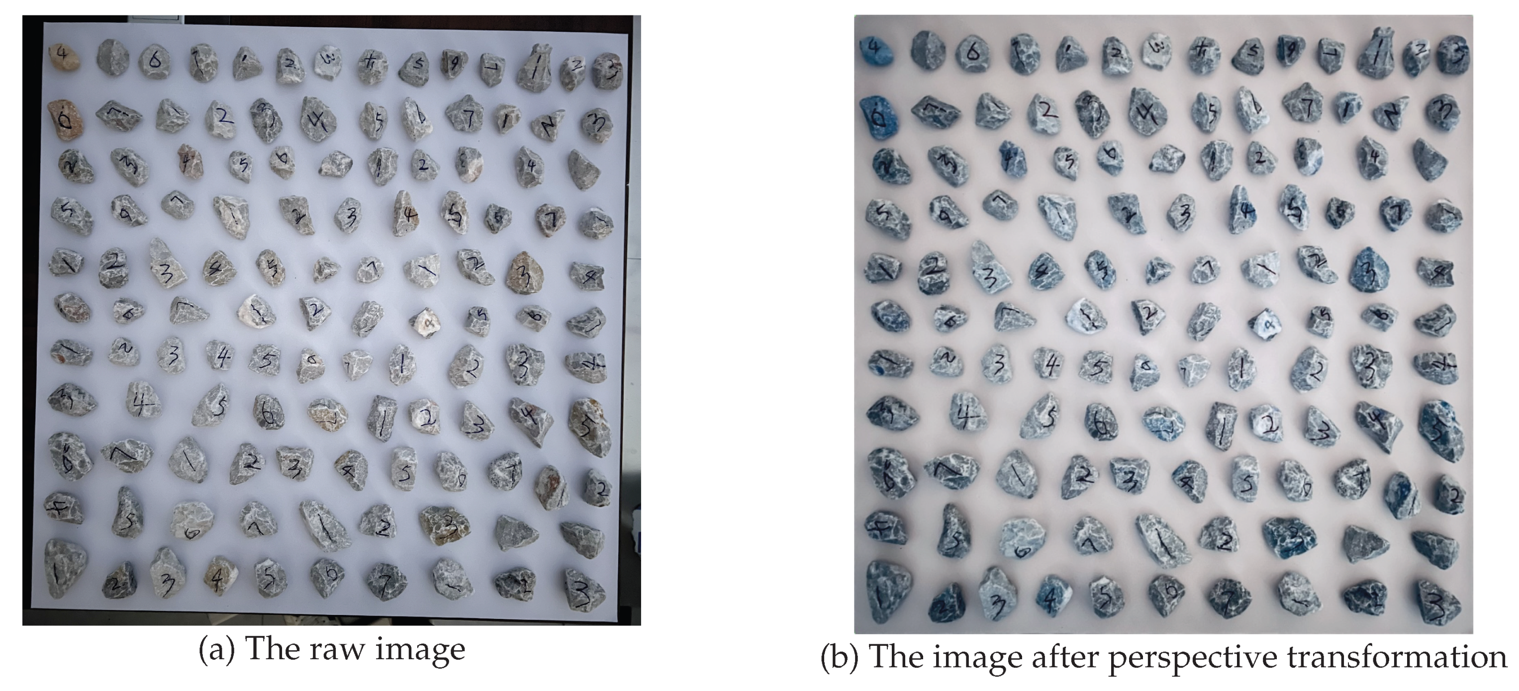
Moreover, since a single photo could not capture all aggregates of each group, multiple shots are taken for each group. This practice ensures a comprehensive record of the distribution and characteristics of the aggregate particles, avoiding any loss of information.
5. Experiment
Implementation environment: Our experiments are implemented in the following environment:
- Hardware environment: The experiments are performed on a computer equipped with an NVIDIA Quadro P2000 GPU, an Intel Core i7-8700K CPU, 16GB of RAM, and the Windows 10 operating system.
- Software environment: The experiments are based on the PyTorch framework under Python 3.10.
Dataset: In this study, we utilize our curated aggregate image dataset. For a comprehensive evaluation, we introduce random seeds and K-fold cross-validation. The code is executed multiple times, and each time the code runs with a different random seed. Based on this, K-fold cross-validation is applied, dividing the dataset into K equal-sized, mutually exclusive subsets. Each fold corresponds to a test set that includes model predictions for each aggregate’s particle size and volume results. K-fold cross-validation enables full utilization of the dataset by allowing each data point to be evaluated sufficiently.
Segmentation and post-processing: During the experiment, we employ SAM for segmentation. To ensure the accuracy of the synthetic gradation curves, we also slightly post-process the segmentation results obtained by SAM with a few interactive mouse-click correction to the contour of the mask. As Figure 10(a) shows, SAM is indeed powerful in terms of providing an accurate segmentation. There are significant variations in particle shape and size, but SAM still demonstrates the ability to accurately segment nearly all aggregates. Moreover, it can tell the shadow from the aggregate well. In Figure 10(b), a few mis-segmented places, such as the bottom left and bottom right, are corrected. Figure 10(c) shows that SAM can perform well in segmenting tiny aggregates. By visualizing the segmented mask images, it is evident that the model exhibits exceptional capability in capturing the edges of aggregate particles.
Predicting the category and volume of an aggregate: KAN predicts the gradation category and volume of each aggregate. As presented in Table 2, classification performance exhibits disparities across gradation categories due to class imbalance. Categories 1–3, with fewer aggregate samples, demonstrate lower precision, recall, and F1-scores compared to categories 4–7. The overall accuracy is 78%. Considering that two-dimensional information are limited to characterize the 3D stones, this level of individual accuracy actually confirms the general effectiveness of KAN.
A scatter plot (as shown in Figure 11) visualizes the deviation between the predicted and actual volumes, where the vertical axis represents the percentage deviation rate, the horizontal axis indexes individual aggregates, and distinct colors denote different gradation categories. Additionally, Table 3 presents the deviation rates between actual and predicted volumes for each aggregate category. The standard deviation indicates a high degree of data dispersion, suggesting significant fluctuations. This limitation arises because the input for the KAN relies on binary masks, which inadequately capture the full geometric features of irregular polyhedral aggregates, offering only partial single-view representations and thus compromising prediction reliability.
However, the deviations exhibit a symmetrical distribution, where positive and negative errors across gradation categories cancel out around a central mean value. This cancellation effect manifests that, at the population level, the mean deviation rate is substantially smaller than the standard deviation, demonstrating statistically significant error mitigation. Consequently, leveraging this error cancellation mechanism inherent to ensemble statistics allows effective circumvention of single-particle prediction uncertainties, which can generate an accurate judgment for the gradation curve.
Judge the gradation curve: KAN assesses 1,000 gradation curves and successfully predicts 858 of them, which validates the accuracy and effectiveness of the model. To visually illustrate the prediction performance, Figure 12 presents an overview of these gradation curves, where the solid blue line represents the actual mean values of the curves, the red dashed line indicates the predicted mean values, and the shaded bandwidth regions reflect their respective variability ranges. These quantitative metrics correspond to the mean values and standard deviations presented in Table 4. Notably, [30] exclusively regulates the gradation parameters for sieve openings of 53mm, 37.5mm, 19mm, 9.5mm, and 4.75mm. Accordingly, our gradation assessment specifically targets these key sieve dimensions.
Figure 13 presents the distribution of deviations between the actual and predicted passing percentages for key sieve sizes using a violin plot. The plot is annotated with the extreme values, third quartile (Q3), median, and first quartile (Q1) of these deviations, providing an intuitive reflection of the model’s predictive discrepancies across different particle sizes. As the particle size decreases, the dispersion increases. The width of the violin indicates the density of data points, with a wider width signifying higher concentration. It can be observed that the prediction performance for Category 1 is satisfactory, with over 95% of the data having deviation values within . For Category 4, the data deviation is controlled within the range. In contrast, the prediction performance for Category 6 is relatively poor, with 20.32% of the data falling within the to deviation range and 1.39% of the data within the to deviation range.
6. Discussion
6.1. Impact of Architecture in KAN
Here, we explore the impact of the KAN’s different architectures on the performance of pre-screening. We evaluate both 2-layer and 3-layer structures, with neuron counts per layer ranging from 8 to 32. As illustrated in Figure 14, different network structures are evaluated for the aggregate regression task. The optimal performance is achieved with 2 hidden layers (16, 16 neurons), yielding a standard deviation of 27.75% between actual and predicted volumesand a mean deviation of -2.49%. Interestingly, in classification tasks, the weighted average (Weighted Avg) remains consistent at 78% across all tested architectures, suggesting that classification performance is insensitive to hidden layer depth and neuron count. More layers may lead to overfitting, considering that KAN has a strong approximation capability.
6.2. Non-Invasiveness of Deep Grading
The non-destructive nature of deep grading—a method leveraging advanced imaging, sensor technologies, and deep learning—eliminates the need for physical handling or mechanical processing of aggregates. Traditional grading techniques, such as sieving or manual sorting, often subject samples to friction, impact, or compression, which can alter particle shape, induce microfractures, or dislodge surface features. These alterations risk destructing the sample, particularly for rare, fragile, or irreplaceable materials. For instance, in extraterrestrial exploration scenarios like analyzing lunar regolith to assess its suitability for construction (e.g., 3D-printed habitats or radiation-shielding structures), physical manipulation could destroy critical information about grain morphology, mineral composition, or electrostatic properties—factors vital for engineering lunar infrastructure. In contrast, deep grading enables the initial judgement of size and shape without contact. This capability is invaluable for limited or high-value samples, where even minor damage could invalidate downstream analyses or deplete scarce resources.
7. Conclusion
This study has introduced deep grading, a framework integrating SAM and KAN, for non-destructive pre-screening of aggregate quality. Rigorous dataset curation and experiments validate that deep grading achieves >80% accuracy in compliance prediction for aggregate clusters. Future research should prioritize dataset diversification and scaling to enhance segmentation precision. Innovations in multi-modal data fusion (e.g., integrating spectral or texture analysis) and adaptive segmentation algorithms could refine screening robustness. Furthermore, model compression techniques—such as quantization or knowledge distillation—would broaden the framework’s utility in resource-constrained industrial environments.
Funding
This work was supported by the Guangxi Science and Technology Program (Grant No. AB24010352).
References
- Fang, M.; Park, D.; Singuranayo, J.L.; Chen, H.; Li, Y. Aggregate gradation theory, design and its impact on asphalt pavement performance: a review. International Journal of Pavement Engineering 2019, 20, 1408–1424. [Google Scholar] [CrossRef]
- Bruno, L.; Parla, G.; Celauro, C. Image analysis for detecting aggregate gradation in asphalt mixture from planar images. Construction and Building Materials 2012, 28, 21–30. [Google Scholar] [CrossRef]
- Reyes-Ortiz, O.J.; Mejia, M.; Useche-Castelblanco, J.S. Digital image analysis applied in asphalt mixtures for sieve size curve reconstruction and aggregate distribution homogeneity. International Journal of Pavement Research and Technology 2021, 14, 288–298. [Google Scholar] [CrossRef]
- Peres, R.S.; Jia, X.; Lee, J.; Sun, K.; Colombo, A.W.; Barata, J. Industrial artificial intelligence in industry 4.0-systematic review, challenges and outlook. IEEE access 2020, 8, 220121–220139. [Google Scholar] [CrossRef]
- Gong, J.; Liu, Z.; Nie, J.; Cui, Y.; Jiang, J.; Ou, X. Study on the automated characterization of particle size and shape of stacked gravelly soils via deep learning. Acta Geotechnica 2025, 1–26. [Google Scholar] [CrossRef]
- Sun, Z.; Li, Y.; Pei, L.; Li, W.; Hao, X. Classification of coarse aggregate particle size based on deep residual network. Symmetry 2022, 14, 349. [Google Scholar] [CrossRef]
- Kirillov, A.; Mintun, E.; Ravi, N.; Mao, H.; Rolland, C.; Gustafson, L.; Xiao, T.; Whitehead, S.; Berg, A.C.; Lo, W.Y.; et al. Segment anything. In Proceedings of the Proceedings of the IEEE/CVF international conference on computer vision, 2023; pp. 4015–4026. [Google Scholar]
- Ravi, N.; Gabeur, V.; Hu, Y.T.; Hu, R.; Ryali, C.; Ma, T.; Khedr, H.; Rädle, R.; Rolland, C.; Gustafson, L.; et al. Sam 2: Segment anything in images and videos. arXiv 2024, arXiv:2408.00714 2024. [Google Scholar]
- Liu, Z.; Wang, Y.; Vaidya, S.; Ruehle, F.; Halverson, J.; Soljačić, M.; Hou, T.Y.; Tegmark, M. Kan: Kolmogorov-arnold networks. arXiv 2024, arXiv:2404.19756 2024. [Google Scholar]
- Weng, Y.; Li, M.; Tan, M.J.; Qian, S. Design 3D printing cementitious materials via Fuller Thompson theory and Marson-Percy model. Construction and Building Materials 2018, 163, 600–610. [Google Scholar] [CrossRef]
- Ma, H.; Xu, W.; Li, Y. Random aggregate model for mesoscopic structures and mechanical analysis of fully-graded concrete. Computers & Structures 2016, 177, 103–113. [Google Scholar]
- Tafesse, S.; Fernlund, J.; Bergholm, F. Digital sieving-Matlab based 3-D image analysis. Engineering Geology 2012, 137, 74–84. [Google Scholar] [CrossRef]
- Thaker, P.; Arora, N. Measurement of Aggregate Size and Shape Using Image Analysis. In Proceedings of the National Conference on Structural Engineering and Construction Management; 2020. [Google Scholar]
- Wang, D.; Wang, H.; Bu, Y.; Schulze, C.; Oeser, M. Evaluation of aggregate resistance to wear with Micro-Deval test in combination with aggregate imaging techniques. Wear 2015, 338, 288–296. [Google Scholar] [CrossRef]
- Prabha, D.S.; Kumar, J.S. Performance evaluation of image segmentation using objective methods. Indian J. Sci. Technol 2016, 9, 1–8. [Google Scholar]
- Yu, Y.; Wang, C.; Fu, Q.; Kou, R.; Huang, F.; Yang, B.; Yang, T.; Gao, M. Techniques and challenges of image segmentation: A review. Electronics 2023, 12, 1199. [Google Scholar] [CrossRef]
- Li, Z.; Liu, F.; Yang, W.; Peng, S.; Zhou, J. A survey of convolutional neural networks: analysis, applications, and prospects. IEEE transactions on neural networks and learning systems 2021, 33, 6999–7019. [Google Scholar] [CrossRef] [PubMed]
- Ronneberger, O.; Fischer, P.; Brox, T. U-net: Convolutional networks for biomedical image segmentation. In Proceedings of the Medical image computing and computer-assisted intervention–MICCAI 2015: 18th international conference, Munich, Germany,October 5-9, 2015, proceedings, part III 18. Springer, 2015; pp. 234–241.
- He, K.; Gkioxari, G.; Dollár, P.; Girshick, R. Mask r-cnn. In Proceedings of the Proceedings of the IEEE international conference on computer vision, 2017; pp. 2961–2969. [Google Scholar]
- Patra, S.; Panda, S.; Parida, B.K.; Arya, M.; Jacobs, K.; Bondar, D.I.; Sen, A. Physics informed kolmogorov-arnold neural networks for dynamical analysis via efficent-kan and wav-kan. arXiv, 2024; arXiv:2407.18373 2024. [Google Scholar]
- Zhang, X.; Zhou, H. Generalization bounds and model complexity for kolmogorov-arnold networks. arXiv, 2024; arXiv:2410.08026 2024. [Google Scholar]
- Xu, K.; Chen, L.; Wang, S. Kolmogorov-arnold networks for time series: Bridging predictive power and interpretability. arXiv, 2024; arXiv:2406.02496 2024. [Google Scholar]
- Li, C.; Liu, X.; Li, W.; Wang, C.; Liu, H.; Liu, Y.; Chen, Z.; Yuan, Y. U-kan makes strong backbone for medical image segmentation and generation. In Proceedings of the Proceedings of the AAAI Conference on Artificial Intelligence, 2025, Vol. 39, pp. 4652–4660.
- Dosovitskiy, A.; Beyer, L.; Kolesnikov, A.; Weissenborn, D.; Zhai, X.; Unterthiner, T.; Dehghani, M.; Minderer, M.; Heigold, G.; Gelly, S.; et al. An Image is Worth 16x16 Words: Transformers for Image Recognition at Scale. In Proceedings of the International Conference on Learning Representations, 2021.
- Brown, T.; Mann, B.; Ryder, N.; Subbiah, M.; Kaplan, J.D.; Dhariwal, P.; Neelakantan, A.; Shyam, P.; Sastry, G.; Askell, A.; et al. Language models are few-shot learners. Advances in neural information processing systems 2020, 33, 1877–1901. [Google Scholar]
- O Pinheiro, P.O.; Collobert, R.; Dollár, P. Learning to segment object candidates. Advances in neural information processing systems 2015, 28. [Google Scholar]
- Radford, A.; Kim, J.W.; Hallacy, C.; Ramesh, A.; Goh, G.; Agarwal, S.; Sastry, G.; Askell, A.; Mishkin, P.; Clark, J.; et al. Learning transferable visual models from natural language supervision. In Proceedings of the International conference on machine learning. PmLR; 2021; pp. 8748–8763. [Google Scholar]
- Bookstein, F.L. Fitting conic sections to scattered data. Computer graphics and image processing 1979, 9, 56–71. [Google Scholar] [CrossRef]
- Ranganathan, A. The levenberg-marquardt algorithm. Tutoral on LM algorithm 2004, 11, 101–110. [Google Scholar]
- for Market Regulation, S.A.; of the People’s Republic of China, S.A. GB/T 14685-2022, Pebble and crushed stone for construction. China Building Materials Federation, Beijng 2022.
- Allgower, E.L.; Schmidt, P.H. Computing volumes of polyhedra. Mathematics of computation 1986, 46, 171–174. [Google Scholar] [CrossRef]
- Szilvśi-Nagy, M.; Matyasi, G. Analysis of STL files. Mathematical and computer modelling 2003, 38, 945–960. [Google Scholar] [CrossRef]
- Hughes, S.; Lau, J. A technique for fast and accurate measurement of hand volumes using Archimedes’ principle. Australasian Physics & Engineering Sciences in Medicine 2008, 31, 56–59. [Google Scholar]
- Hughes, S.W. Archimedes revisited: a faster, better, cheaper method of accurately measuring the volume of small objects. Physics education 2005, 40, 468. [Google Scholar] [CrossRef]
Figure 1.
Compute four geometric quantities (short ax, long ax, area, perimeter) based on the smallest ellipse covering the 2D profile of each aggregate.
Figure 1.
Compute four geometric quantities (short ax, long ax, area, perimeter) based on the smallest ellipse covering the 2D profile of each aggregate.
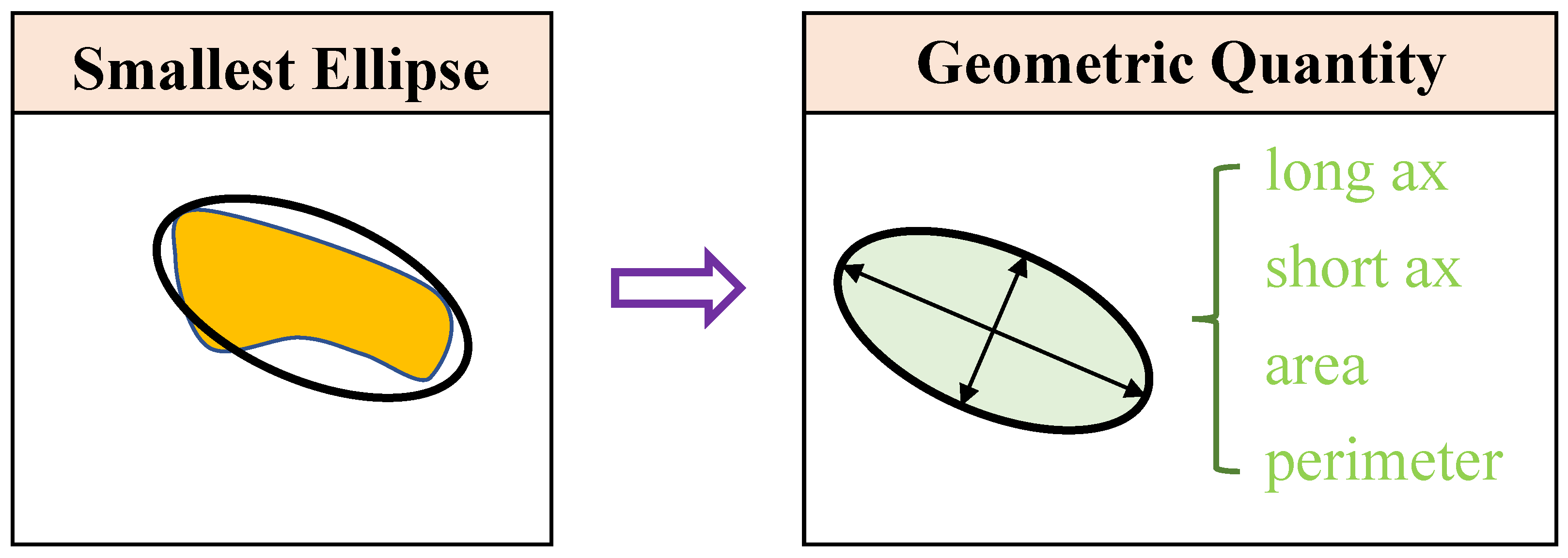
Figure 2.
The basic structure of KAN, where and are parametrized as a linear combination of B-splines whose coefficients are learned.
Figure 2.
The basic structure of KAN, where and are parametrized as a linear combination of B-splines whose coefficients are learned.
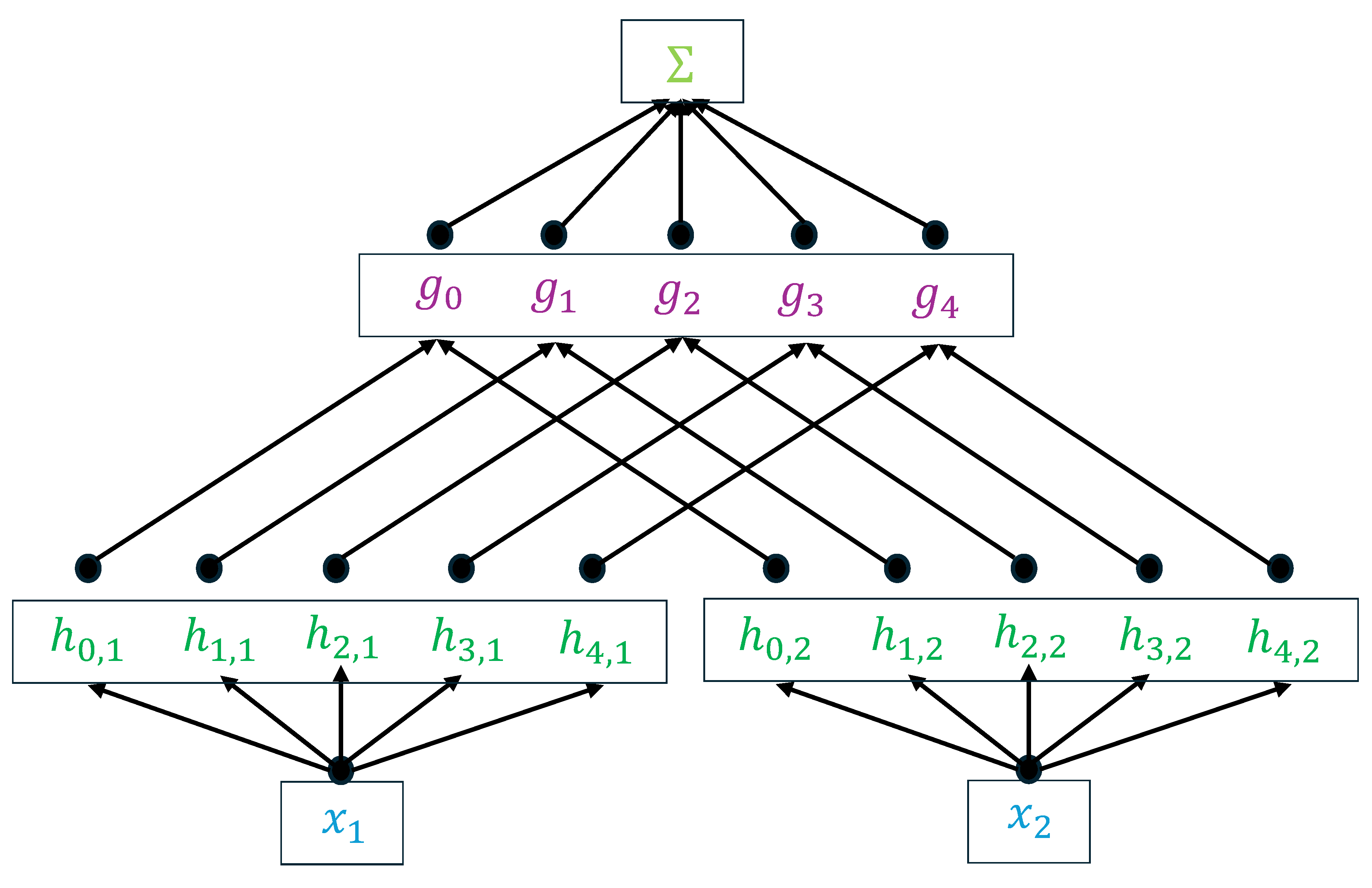
Figure 3.
Drying the aggregate until the weight does not change.

Figure 4.
Aggregate classification by the particle size.
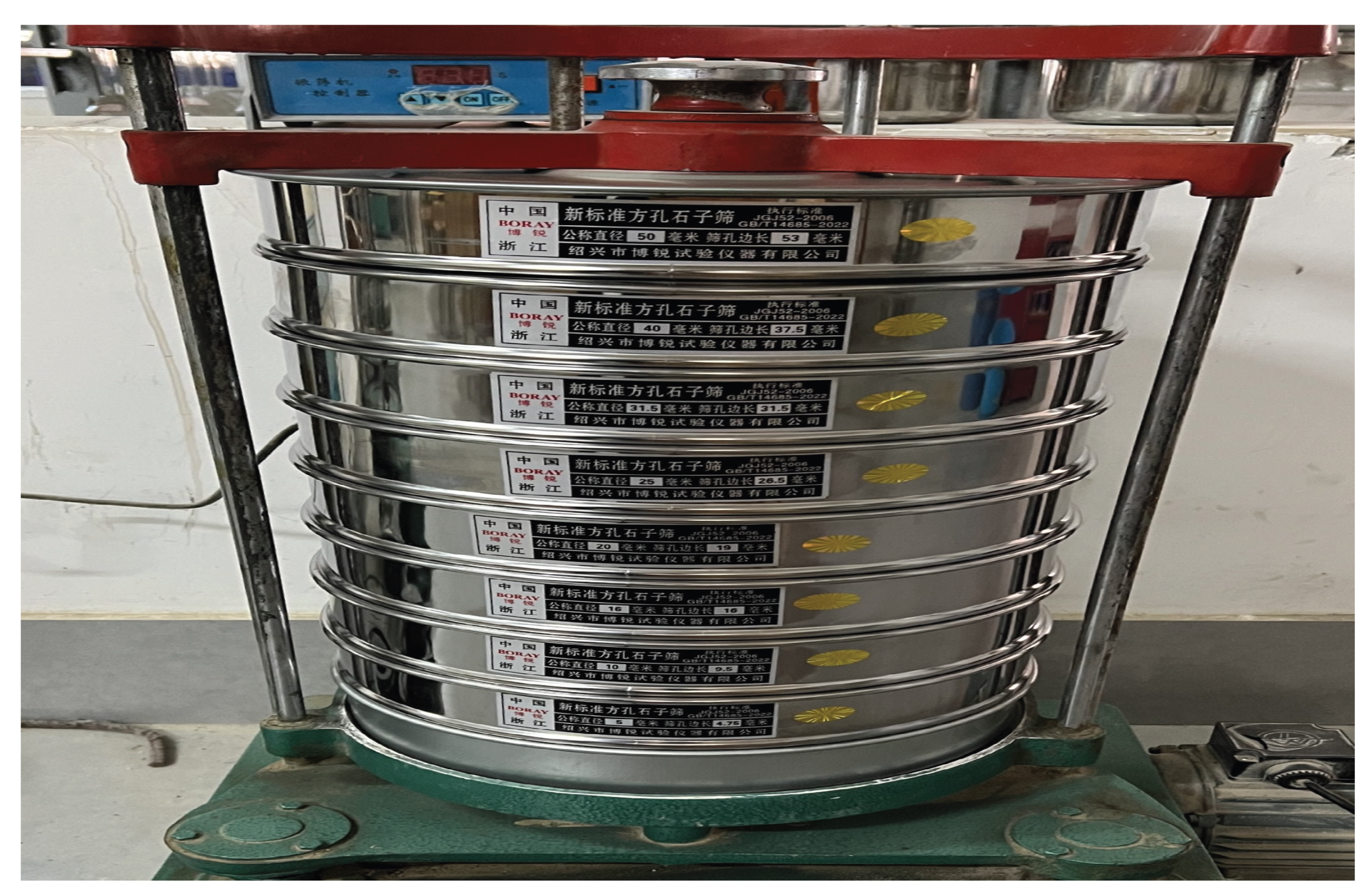
Figure 5.
A single aggregate is scanned to have a 3D geometric measurement.
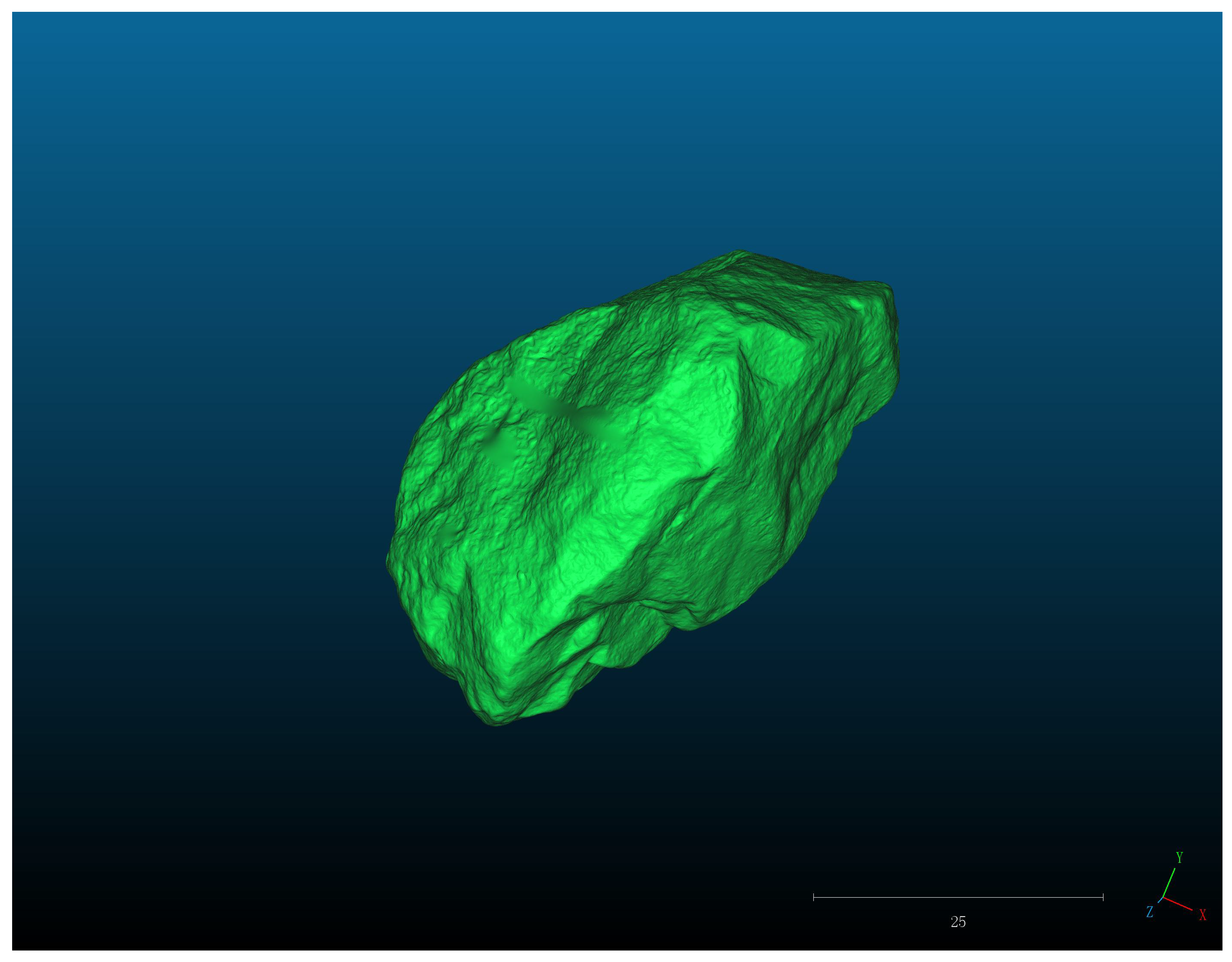
Figure 6.
The image of the buoyancy balance used for the volume measurement.
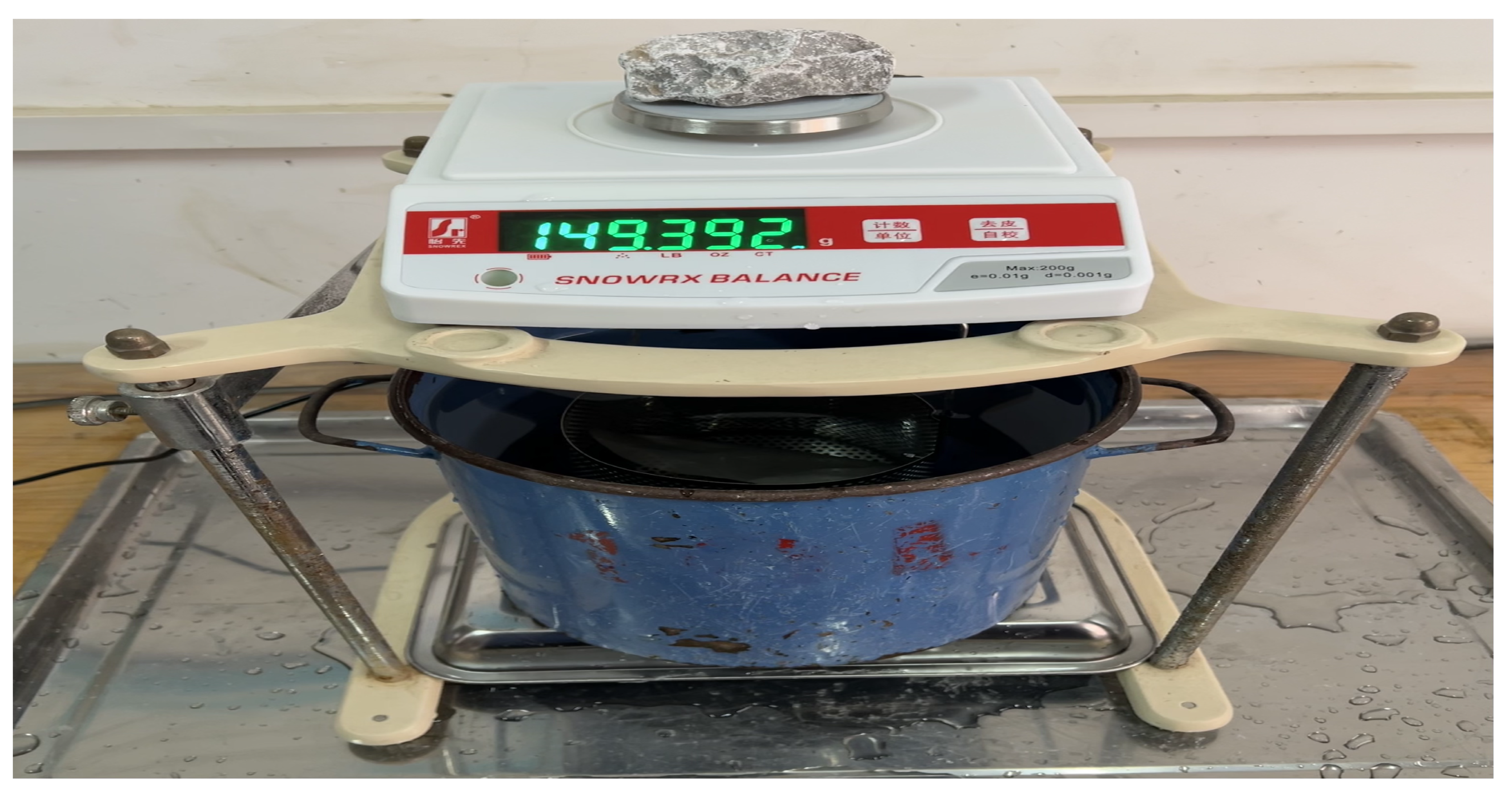
Figure 7.
We contrast the volumes computed from the 3D scan and the buoyant force. The errors in volume are acceptable for large and middle aggregates. In our network training, we take the volume measured by buoyancy as our gold standard.
Figure 7.
We contrast the volumes computed from the 3D scan and the buoyant force. The errors in volume are acceptable for large and middle aggregates. In our network training, we take the volume measured by buoyancy as our gold standard.
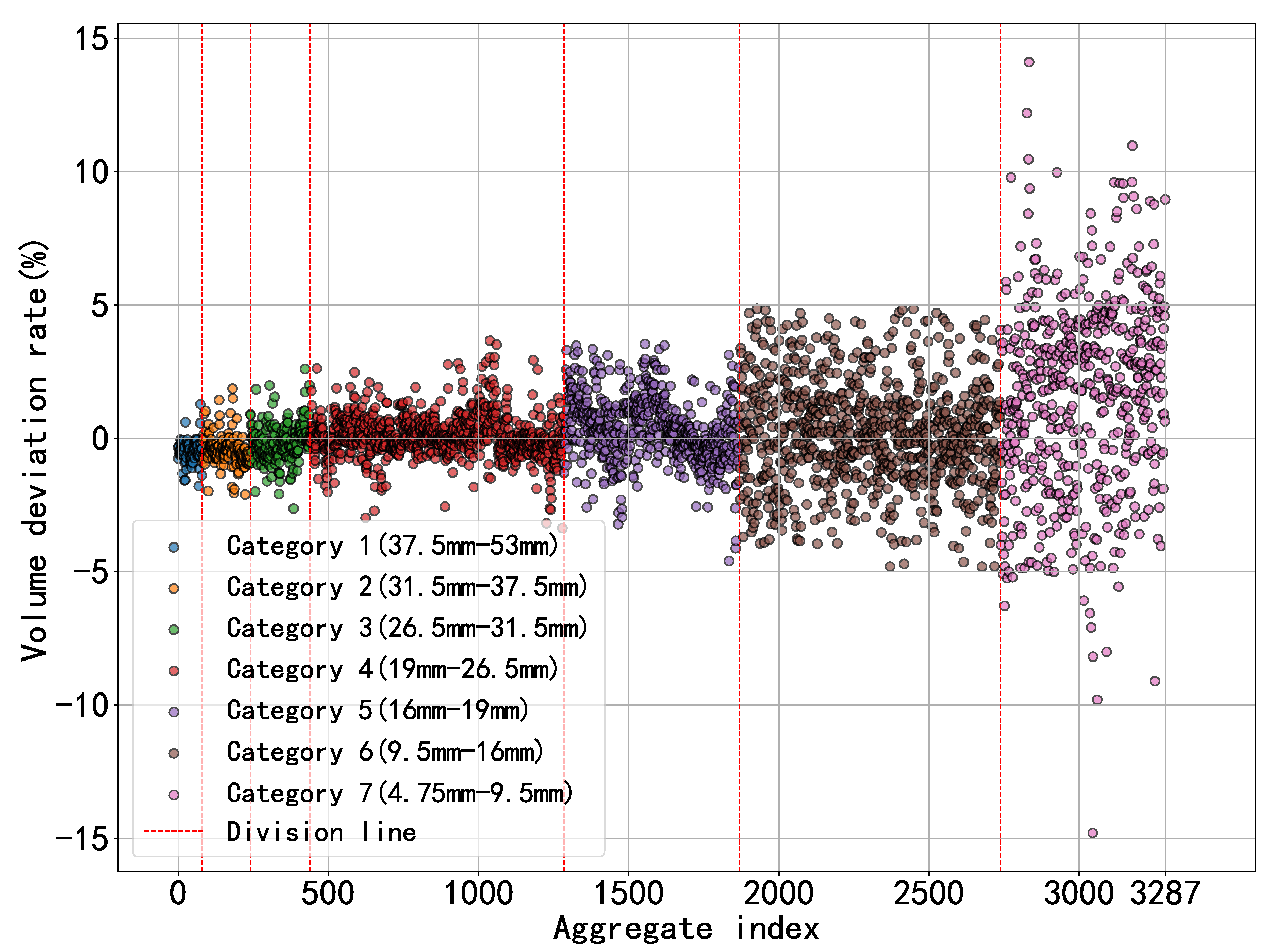
Figure 8.
The histogram of actual passing percentage for key sieve size.
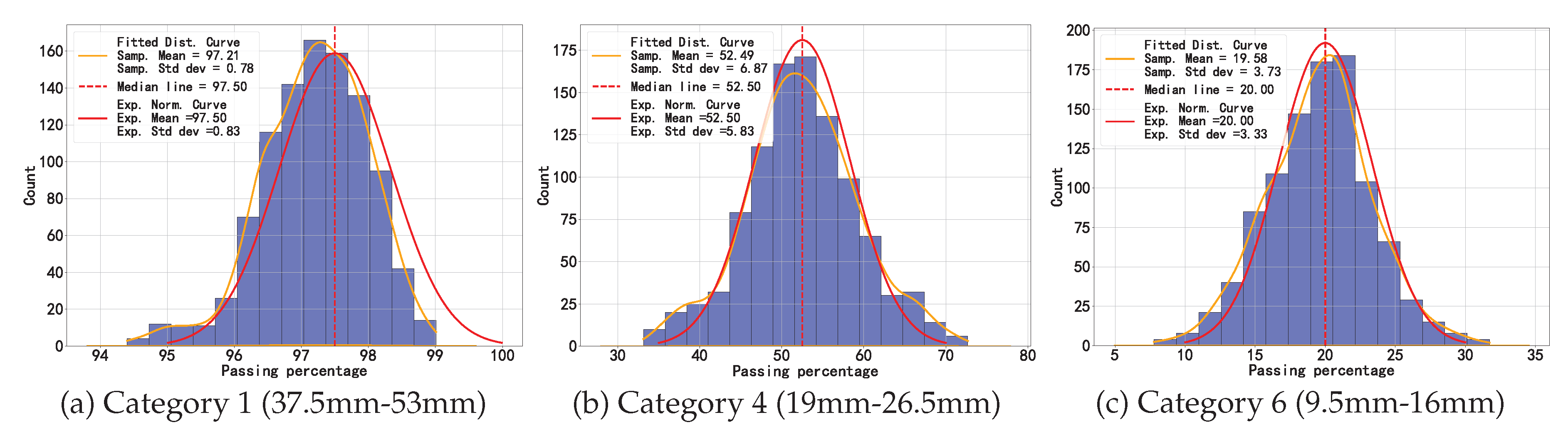
Figure 10.
The segmentation results of the SAM model.
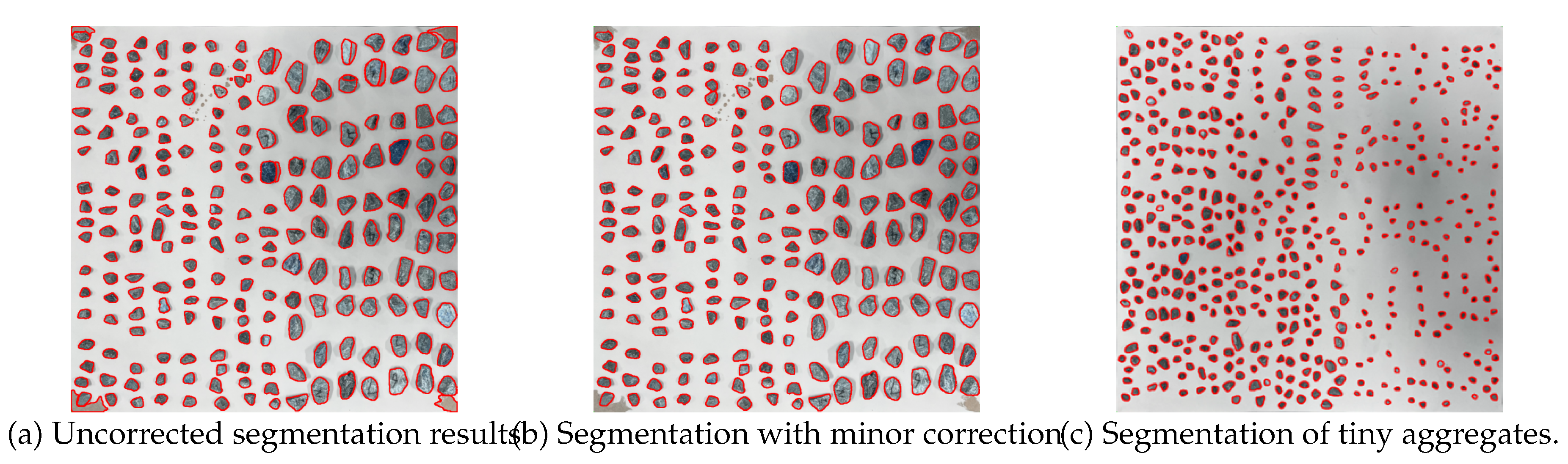
Figure 11.
The error between the predicted and the true volumes. The errors exhibit a symmetrical distribution, where positive and negative errors across gradation categories cancel out around a central mean value.
Figure 11.
The error between the predicted and the true volumes. The errors exhibit a symmetrical distribution, where positive and negative errors across gradation categories cancel out around a central mean value.
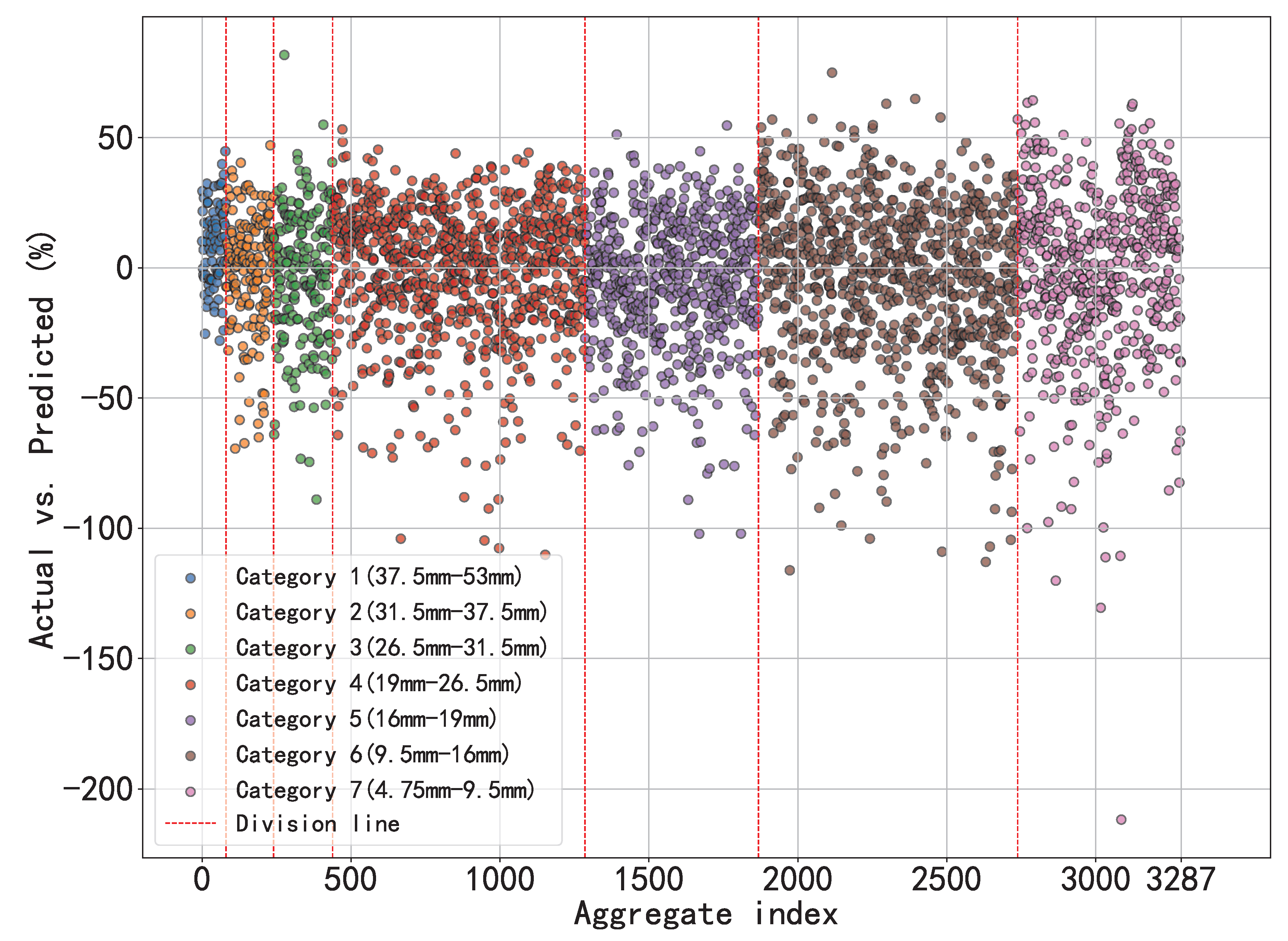
Figure 12.
Composite plot of 1000 gradation curves.
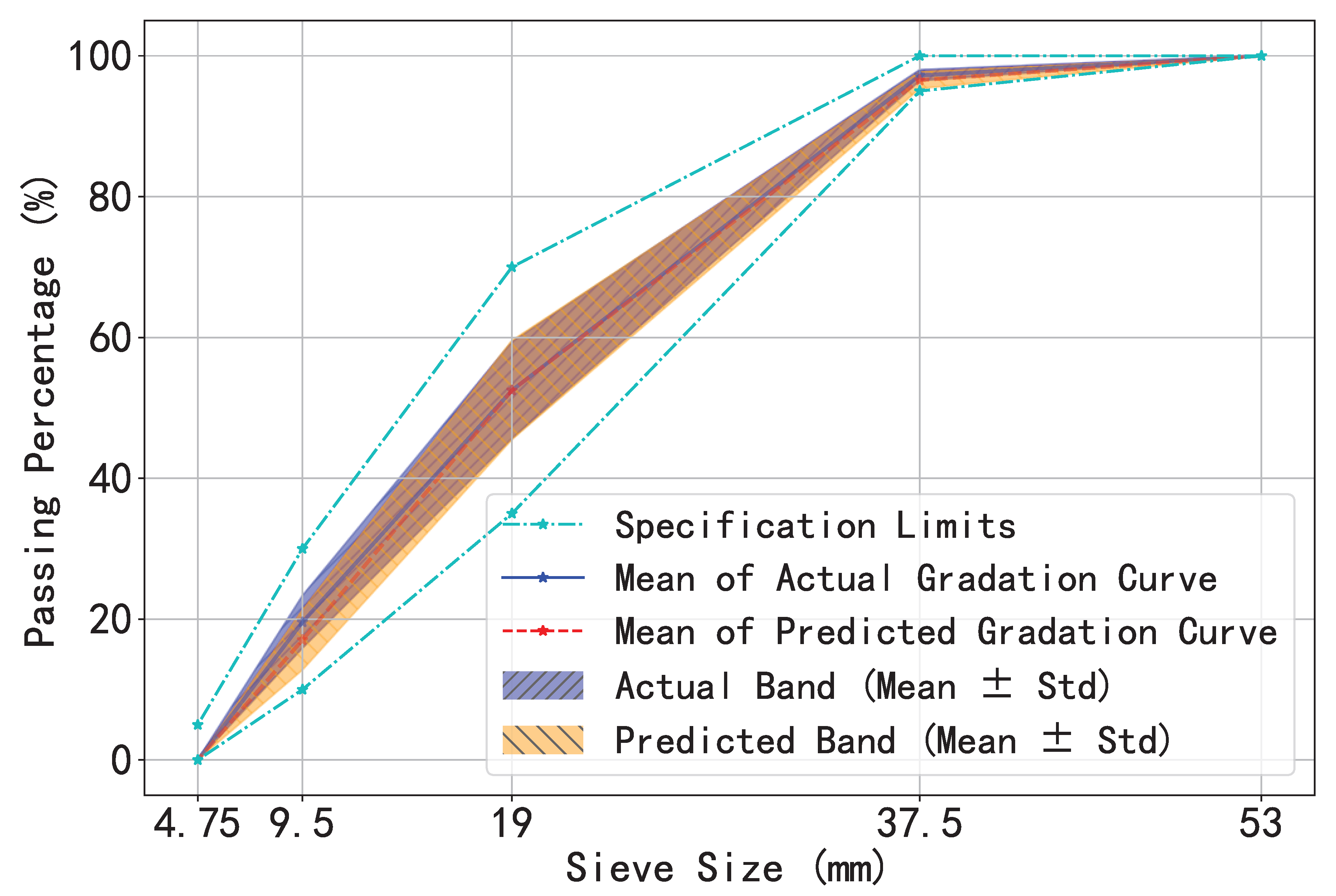
Figure 13.
The distribution of deviations between actual and predicted passing percentages.
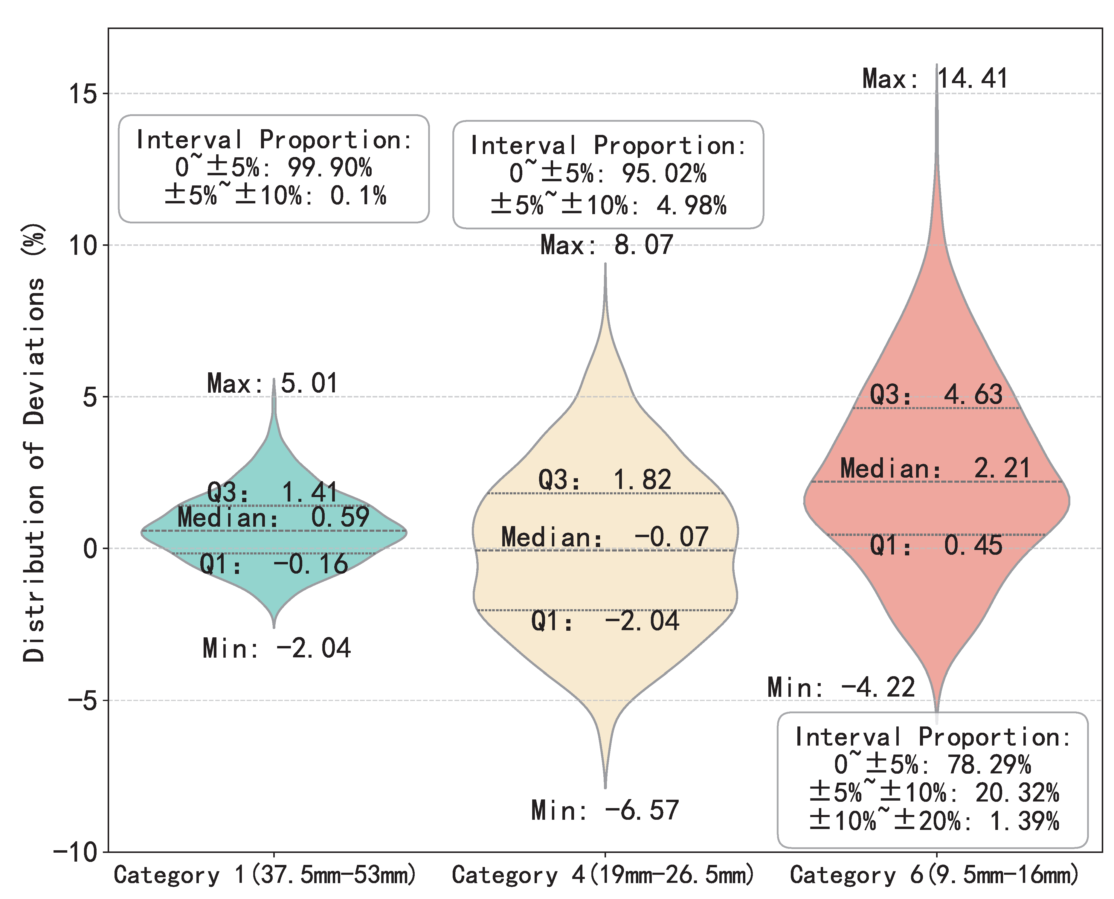
Figure 14.
The prediction deviation of different hidden layer architectures.
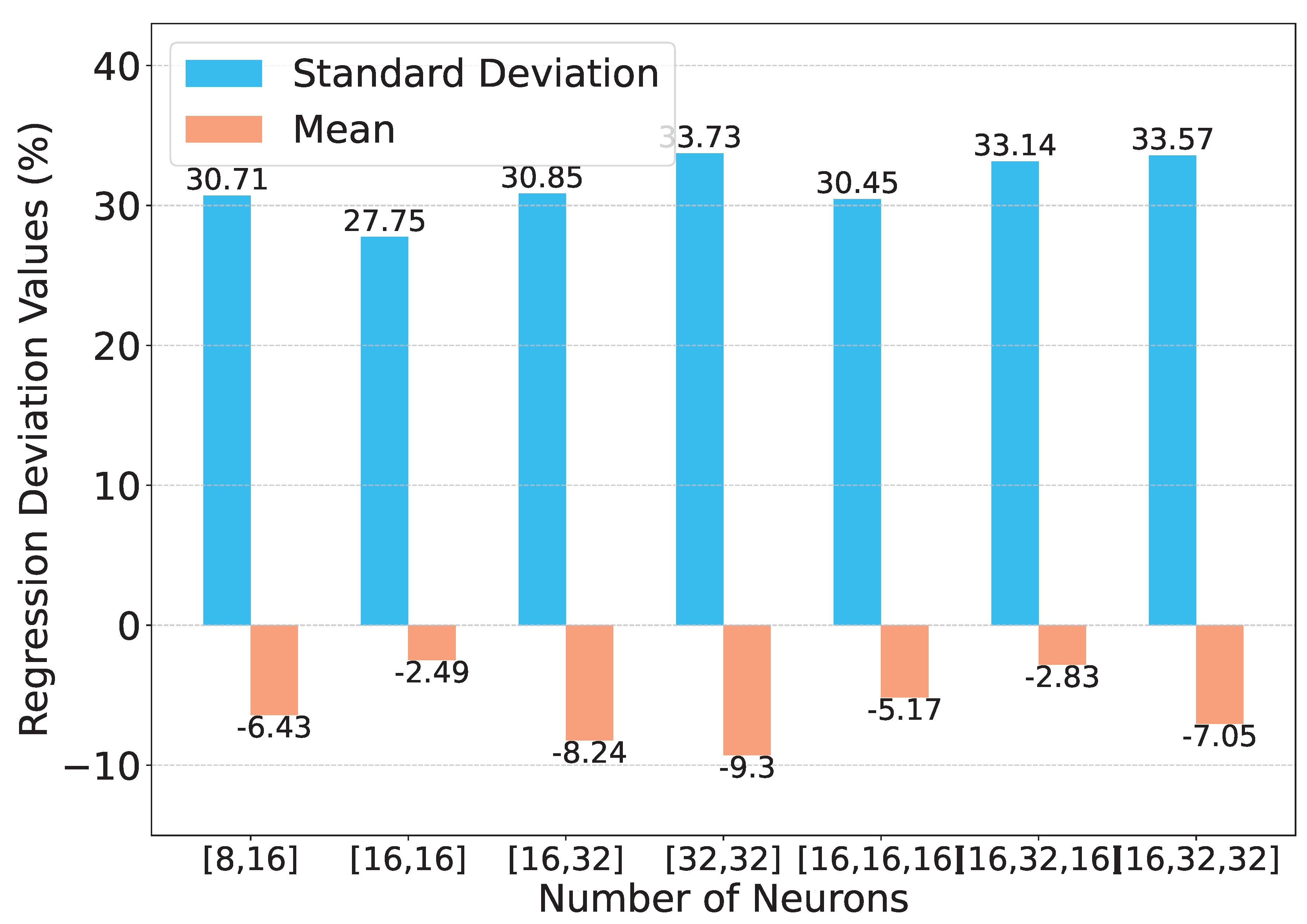

Table 1.
Comparison between traditional and deep grading.
| Cost | Scalability | Environmental Impact | |
|---|---|---|---|
| Traditional | high | low | high |
| Deep | low | high | low |
Table 2.
The classification accuracy (the precision, recall, and F1 score) on the individual aggregate.
Table 2.
The classification accuracy (the precision, recall, and F1 score) on the individual aggregate.
| Category | Precision(%) | Recall(%) | F1 Score(%) | Support |
|---|---|---|---|---|
| 1 (37.5mm-53mm) | 67 | 65 | 66 | 80 |
| 2 (31mm-37.5mm) | 58 | 59 | 58 | 160 |
| 3 (26.5mm-31mm) | 60 | 58 | 59 | 198 |
| 4 (19mm-26.5mm) | 81 | 84 | 82 | 847 |
| 5 (16mm-19mm) | 70 | 69 | 70 | 583 |
| 6 (9.5mm-16mm) | 85 | 81 | 83 | 870 |
| 7 (4.75mm-9.5mm) | 84 | 87 | 85 | 549 |
| accuracy (%) | 78 | 3287 | ||
| macro avg(%) | 72 | 72 | 72 | 3287 |
| weighted avg(%) | 78 | 78 | 78 | 3287 |
Table 3.
The actual vs the predicted volume deviation rate.
| Category | Standard Deviation (%) | Mean Value (%) |
|---|---|---|
| 1 (37.5mm-53mm) | 15.81 | 8.77 |
| 2 (31mm-37.5mm) | 22.48 | -1.61 |
| 3 (26.5mm-31mm) | 25.31 | -3.25 |
| 4 (19mm-26.5mm) | 24.84 | -0.84 |
| 5 (16mm-19mm) | 24.79 | -5.41 |
| 6 (9.5mm-16mm) | 30.26 | -3.89 |
| 7 (4.75mm-9.5mm) | 33.21 | -1.35 |
| Global Data | 27.75 | -2.49 |
Table 4.
The overall quantification of gradation curve
| Category | Actual Passing Percentage | Predicted Passing Percentage | ||
|---|---|---|---|---|
| Mean | Std | Mean | Std | |
| 1 (37.5mm-53mm) | 97.21 | 0.78 | 96.53 | 1.21 |
| 4 (19mm-26.5mm) | 52.49 | 6.87 | 52.50 | 7.02 |
| 6 (9.5mm-16mm) | 19.58 | 3.73 | 17.05 | 4.28 |
Disclaimer/Publisher’s Note: The statements, opinions and data contained in all publications are solely those of the individual author(s) and contributor(s) and not of MDPI and/or the editor(s). MDPI and/or the editor(s) disclaim responsibility for any injury to people or property resulting from any ideas, methods, instructions or products referred to in the content. |
© 2025 by the authors. Licensee MDPI, Basel, Switzerland. This article is an open access article distributed under the terms and conditions of the Creative Commons Attribution (CC BY) license (http://creativecommons.org/licenses/by/4.0/).
Copyright: This open access article is published under a Creative Commons CC BY 4.0 license, which permit the free download, distribution, and reuse, provided that the author and preprint are cited in any reuse.


