On the Geometric Interpretation of Primes via Singularity Theory

1. Introduction

1.1. Research Background and Motivation

Prime numbers have long captivated mathematicians for their fundamental yet elusive nature. Traditionally studied through analytic and algebraic number theory, primes are increasingly being explored from geometric and topological perspectives. Recent advances in arithmetic geometry and the study of schemes have opened new possibilities for interpreting prime numbers as geometric or singular structures within algebraic varieties.

This research is motivated by the hypothesis that prime numbers may correspond to singularities—or regular points—on algebraic varieties defined by certain classes of polynomials. We seek to understand how primes are distributed in relation to the singular loci of these varieties, and to what extent their number-theoretic properties can be interpreted geometrically.

1.2. Review of Prior Research

Historically, the relationship between geometry and prime numbers has been explored through such lenses as:

• Elliptic curves over finite fields, where primes influence the number of rational points;
• Discriminants and resultants, which connect factorization and singularity theory;
• p-adic geometry, providing a local analytic framework to study number-theoretic phenomena;
• Arakelov geometry and Néron models, which model smooth and singular behaviors over arithmetic bases.

However, relatively little work has focused specifically on the direct correspondence between singularities in algebraic geometry and prime numbers as arithmetic objects. Our work attempts to fill this gap by formalizing that connection through singularity theory and the fiber structures of morphisms.

1.3. Research Objectives and Overview

This study aims to:

• Analyze how singular loci and regular points of algebraic varieties correspond to the existence or absence of prime-valued solutions to certain polynomial equations;
• Formulate and prove a series of theorems relating singularity conditions to p-adic local properties and modulo p behavior;
• Explore how singular fibers, discriminants, and resultants reflect arithmetic data such as prime factorization;
• Generalize these findings into a geometric framework where prime distributions can be interpreted as topological or cohomological phenomena.

1.4. Structure of the Paper

This paper is structured as follows:

• Chapter 2 introduces the mathematical background, covering singularity theory, local rings, scheme morphisms, and the number-theoretic roles of discriminants and resultants.
• Chapters 3–8 explore the relationship between primes and singularities, covering local and global perspectives, with each chapter culminating in an original theorem (Theorems A–F).
• Chapter 9 synthesizes the theorems and provides a unifying framework.
• Chapter 10 concludes with a summary and suggestions for future research directions, including potential connections to deep open problems such as the Riemann Hypothesis.

2. Theoretical Background

2.1. Overview of Singularity Theory

Singularity theory studies points on algebraic varieties or manifolds where the usual properties of smoothness or regularity fail. These points, known as singularities, often exhibit exceptional algebraic or geometric behavior and are central objects in both algebraic geometry and differential topology.

In the context of algebraic geometry, singularities of a variety defined by a polynomial $f(x_1,\dots ,x_n)\in \mathbb{C}[x_1,\dots ,x_n]$ can be detected using the vanishing of partial derivatives. Specifically, a point $P\in {\mathbb{C}}^n$ is called a singular point of the hypersurface $V\left(f\right)$ if:

$${\displaystyle \frac{\partial f}{\partial x_1}}\left(P\right)=\dots ={\displaystyle \frac{\partial f}{\partial x_n}}\left(P\right)=0.$$

The set of all such points forms the singular locus of the variety.

Key tools in singularity theory include:

• Jacobian Criterion: A method to detect singularities based on the rank of the Jacobian matrix.
• Zariski Tangent Space: Provides a linear approximation at a point and indicates singularity when its dimension exceeds that of the variety.
• Local Rings: The local ring ${\mathcal{O}}_{X,P}$ at a point $P\in X$ helps determine whether P is regular (i.e., nonsingular).

2.2. Structure of Regular and Singular Local Rings

In algebraic geometry, local rings play a fundamental role in understanding the local behavior of schemes and varieties. The concepts of regular and singular rings are central to classifying points as smooth or singular.

Regular Local Rings: A local ring $(R,\mathfrak{m})$ is called regular if the dimension of the Zariski tangent space $\mathfrak{m}/{\mathfrak{m}}^2$ equals the Krull dimension of R. Equivalently, this means the minimal number of generators of the maximal ideal $\mathfrak{m}$ equals the dimension of the ring:

$${dim}_{\kappa \left(\mathfrak{m}\right)}(\mathfrak{m}/{\mathfrak{m}}^2)=dimR.$$

This condition implies that locally at that point, the variety behaves like a smooth manifold.

Singular Local Rings: If the above condition fails, i.e., the number of generators of $\mathfrak{m}$ exceeds the Krull dimension, then the point is singular, and the local ring is called a singular ring.

2.3. Algebraic Varieties and Fiber Structures

Algebraic varieties form the geometric backbone of modern algebraic geometry. They are defined as the solution sets of systems of polynomial equations and can be studied locally and globally through their structure sheaves and morphisms.

A fiber in algebraic geometry arises when one considers a morphism of schemes $f:X\to S$. For a point $s\in S$, the fiber over s, denoted $X_s$, is the scheme $X{\times }_{S}Spec\left(\kappa \left(s\right)\right)$. This represents the geometric shape of X as seen “over” the point s.

2.4. Arithmetic Applications of Discriminants and Resultants

Discriminants and resultants are classical tools in algebra and number theory that encode subtle information about the roots and singularities of polynomials. In algebraic geometry, they provide a means of detecting where fibers become singular or where multiple roots coalesce.

Discriminants: Given a polynomial $f\left(x\right)\in \mathbb{Z}\left[x\right]$, its discriminant $\Delta \left(f\right)$ is a function of its coefficients that vanishes if and only if the polynomial has a multiple root. For example, if $f\left(x\right)=x^2+bx+c$, then

$$\Delta \left(f\right)=b^2-4c.$$

In general, if $p\mid \Delta \left(f\right)$, then modulo p, the polynomial $f\left(x\right)$ has a multiple root, indicating a singular fiber when f is viewed as part of a family.

3. Polynomial Singular Loci and Prime Correspondence

3.1. Classification of Singular Points via the Jacobian Criterion

To understand the structure of singularities on algebraic varieties, the Jacobian criterion is one of the most fundamental tools. For a polynomial $f(x_1,\dots ,x_n)\in \mathbb{Z}[x_1,\dots ,x_n]$, the singular locus is determined by the vanishing of all first-order partial derivatives.

Jacobian Criterion: A point $P=(a_1,\dots ,a_n)$ on the variety defined by f is singular if:

$${\displaystyle \frac{\partial f}{\partial x_1}}\left(P\right)=\dots ={\displaystyle \frac{\partial f}{\partial x_n}}\left(P\right)=0.$$

This condition ensures that the Jacobian matrix loses rank at P, implying that the tangent space is larger than expected.

3.2. Comparison of Prime Distribution at Regular and Singular Points

A central theme in this study is the comparative behavior of prime-valued solutions at regular versus singular points of a given algebraic variety. The underlying hypothesis is that prime occurrences may correlate with the nature of a point in terms of singularity.

3.3. Conditions and Validity for Primes Corresponding to Singularities

Let $f(x_1,\dots ,x_n)\in \mathbb{Z}[x_1,\dots ,x_n]$ be a polynomial. We consider the following two propositions:

• Proposition 1: The condition required to define a sheaf structure supported only on singular integer solutions that yield prime values.
• Proposition 2: The condition under which a prime-valued integer solution corresponds to a singular point.

3.4. Theorem A: Prime-Valued Solutions Corresponding to Singular Points

Theorem 3.1.

Let $f(x_1,\dots ,x_n)\in \mathbb{Z}[x_1,\dots ,x_n]$ be a polynomial. Suppose there exists a point $\overrightarrow{a}=(a_1,\dots ,a_n)\in {\mathbb{Z}}^n$ such that:

1. 

$\nabla f\left(\overrightarrow{a}\right)=0$, i.e., $\overrightarrow{a}\in Sing\left(f\right)$, and

2. 

$f\left(\overrightarrow{a}\right)=p\in \mathbb{P}$, a prime number,

then the point $\overrightarrow{a}$ is a singular integer solution corresponding to a prime value. Moreover, such a solution validates both a geometric and arithmetic condition simultaneously.

Proof. 

By hypothesis, $\nabla f\left(\overrightarrow{a}\right)=0$, which by the Jacobian criterion implies that $\overrightarrow{a}$ lies in the singular locus of the variety $V\left(f\right)$. Since $f\left(\overrightarrow{a}\right)=p\in \mathbb{P}$, this point yields a prime output. Thus, $\overrightarrow{a}\in {\mathbb{Z}}^n\cap Sing\left(f\right)$, and $f\left(\overrightarrow{a}\right)\in \mathbb{P}$, completing the construction of a prime-valued singular integer solution.

Example: Let $f(x,y)=x^5-3x+y^5$. Then:

$${\displaystyle \frac{\partial f}{\partial x}}=3x^2-3,{\displaystyle \frac{\partial f}{\partial y}}=5y^4.$$

Solving $\nabla f=0$ yields $x=\pm 1$, $y=0$. Evaluating:

$$f(-1,0)=-1+3=2\in \mathbb{P}.$$

Hence, $(-1,0)$ is a singular point with a prime output, illustrating the theorem. □

4. Arithmetic Interpretation of Singularities

4.1. Prime Conditions Interpreted via Local Rings

In number theory and algebraic geometry, local rings provide a lens through which one can analyze the behavior of functions and varieties “near” a given point. When considering prime numbers, it is natural to examine the localization of the integers at a prime p, written ${\mathbb{Z}}_{\left(p\right)}$, which forms a discrete valuation ring (DVR).

4.2. Analysis of Singularity Existence Under p-adic Conditions

p-adic analysis provides a powerful tool for understanding the behavior of polynomial equations near prime-related conditions. Suppose we have $f\left(\overrightarrow{x}\right)\in {\mathbb{Z}}_p\left[\overrightarrow{x}\right]$, and there exists $\overrightarrow{a}\in {\mathbb{Z}}_p^n$ such that:

$$\nabla f\left(\overrightarrow{a}\right)\equiv 0(modp)\mathrm{and}f\left(\overrightarrow{a}\right)\in p{\mathbb{Z}}_p.$$

Then $\overrightarrow{a}$ is a p-adic singular point in the reduction of $fmodp$, and the valuation of $f\left(\overrightarrow{a}\right)$ relates closely to the singular locus structure in arithmetic geometry.

4.3. Refined Theorem B: p-adic Conditions and Geometric Singularities

Theorem 4.1

(Refined Theorem B). Let $f(x_1,\dots ,x_n)\in \mathbb{Z}[x_1,\dots ,x_n]$ and let $p\in \mathbb{P}$ be a prime number. Suppose there exists a point $\mathbf{a}=(a_1,\dots ,a_n)\in {\mathbb{Z}}_p^n$ such that:

1. 

$f\left(\mathbf{a}\right)\in p{\mathbb{Z}}_p$,

2. 

$\nabla f\left(\mathbf{a}\right)\equiv 0(modp)$,

3. 

Each $a_i\equiv 0(modp)$.

Then the reduction $\overline{\mathbf{a}}\in {\mathbb{F}}_p^n$ is a singular point of the reduction $fmodp$, and hence corresponds to a singular point in the fiber $X_p$ of the scheme $Spec\left(\mathbb{Z}\right[\mathbf{x}]/\langle f\rangle )\to Spec\left(\mathbb{Z}\right)$.

Proof. 

Given the conditions:

• $f\left(\mathbf{a}\right)\in p{\mathbb{Z}}_p$ implies $f\left(\overline{\mathbf{a}}\right)\equiv 0(modp)$ in ${\mathbb{F}}_p$.
• $\nabla f\left(\mathbf{a}\right)\equiv 0(modp)$ implies $\nabla f\left(\overline{\mathbf{a}}\right)=0$ in ${\mathbb{F}}_p$, since each partial derivative ${\displaystyle \frac{\partial f}{\partial x_i}}\left(\mathbf{a}\right)\in p{\mathbb{Z}}_p$.
• $a_i\equiv 0(modp)$ ensures $\overline{\mathbf{a}}=(0,\dots ,0)$.

By the Jacobian criterion, $\overline{\mathbf{a}}$ is a singular point of $fmodp$, as $\nabla f\left(\overline{\mathbf{a}}\right)=0$ and $f\left(\overline{\mathbf{a}}\right)=0$. To confirm this singularity cannot be lifted to a smooth point, we apply Hensel’s Lemma. For a polynomial $g\left(x\right)\in {\mathbb{Z}}_p\left[x\right]$ with a root $a\in {\mathbb{F}}_p$ such that $g\left(a\right)\equiv 0(modp)$ and $g^{\prime }\left(a\right)\neg \equiv 0(modp)$, Hensel’s Lemma guarantees a unique lift to ${\mathbb{Z}}_p$. Here, since $\nabla f\left(\overline{\mathbf{a}}\right)=0$, the derivative condition fails, preventing a smooth lift. Thus, $\overline{\mathbf{a}}$ remains a genuine singularity in the fiber $X_p$.

Example: Consider $f(x,y)=x^3+y^4-p\in \mathbb{Z}[x,y]$ at $(0,0)\in {\mathbb{Z}}_p^2$. Compute:

$$f(0,0)=-p\in p{\mathbb{Z}}_p,{\displaystyle \frac{\partial f}{\partial x}}=3x^2,{\displaystyle \frac{\partial f}{\partial y}}=4y^3.$$

At $(0,0)$, $\nabla f(0,0)=(0,0)(modp)$, satisfying condition (2). Since $(0,0)\equiv (0,0)(modp)$, condition (3) holds, and $f(0,0)\in p{\mathbb{Z}}_p$ satisfies condition (1). Thus, $(0,0)$ is a singular point in $X_p=Spec({\mathbb{F}}_p[x,y]/(x^3+y^4))$. □

5. Interpretation of Primes via Algebraic Fiber Structures

5.1. Conditions for the Emergence of Singular Fibers Under Morphisms

Let $f:X\to Spec\left(\mathbb{Z}\right)$ be a morphism of schemes, where X is defined by a polynomial $f(x,y)=x^2+y^2-p$, with p a prime number. For each point $\mathfrak{p}=\langle p\rangle \in Spec\left(\mathbb{Z}\right)$, the fiber $X_p$ is defined by reducing the equation modulo p.

5.2. Refined Analysis of Singular Structure in $f(x,y)=x^2+y^2-p$

Definition 5.1.

A point $(x_0,y_0)\in {\mathbb{F}}_p^2$ is a singular point of the fiber $X_p$ if:

$$f_p(x_0,y_0)=0\mathrm{and}\nabla f_p(x_0,y_0)=(2x_0,2y_0)=(0,0).$$

Thus, the only candidate is $(0,0)$, and we check:

$$f_p(0,0)=-p\equiv 0(modp)\Rightarrow (0,0)\in X_p\mathrm{and}\mathrm{is}\sin \mathrm{gular}.$$

Theorem 5.2.

Let $f(x,y)=x^2+y^2-p$ and $X_p$ the fiber over p in $Spec\left(\mathbb{Z}\right)$. Then:

1. 

$\langle 0,0\rangle$ is a singular point in $X_p$ for all primes p.

2. 

The geometric structure of $X_p$ near $(0,0)$ is determined by the quadratic character of $-1$ modulo p.

Proof. 

Since $\nabla f=(2x,2y)$, the singularity occurs precisely at $x=y=0$. Also, $f(0,0)=-p\equiv 0(modp)$, hence the point lies on the fiber. The solution set of $x^2+y^2=0(modp)$ is nontrivial if and only if $-1$ is a quadratic residue modulo p:

$$\left({\displaystyle \frac{-1}{p}}\right)=1\iff p\equiv 1(mod4).$$

□

Corollary 5.3.

If $p\equiv 1(mod4)$, then $X_p$ contains multiple ${\mathbb{F}}_p$-points satisfying $x^2+y^2=0$, and the singularity at $(0,0)$ is non-isolated. Otherwise, if $p\equiv 3(mod4)$, $(0,0)$ is the only point on $X_p$ and the singularity is isolated.

5.3. Refined Theorem C: Prime-Induced Singular Fibers

Theorem 5.4

(Refined Theorem C). Let $f(x,y)=x^2+y^2-p$ with p a prime, and consider the arithmetic scheme $X\to Spec\left(\mathbb{Z}\right)$ defined by $f=0$. Let $X_p$ denote the fiber over the prime p. Then:

1. 

$X_p$ is singular at the origin $(0,0)\in {\mathbb{F}}_p^2$ for every p.

2. 

The nature of the singularity at $(0,0)$ depends on the value of $p(mod4)$:

• If $p\equiv 1(mod4)$, then $-1$ is a quadratic residue in ${\mathbb{F}}_p$, and $x^2+y^2\equiv 0(modp)$ has multiple solutions. The singularity is non-isolated.
• If $p\equiv 3(mod4)$, then $-1$ is a non-residue, and the only solution to $x^2+y^2\equiv 0(modp)$ is $(0,0)$. The singularity is isolated.
• If $p=2$, the equation $x^2+y^2\equiv 0(mod2)$ has a single solution $(0,0)$, and the singularity is isolated, similar to the $p\equiv 3(mod4)$ case.

Proof. 

The fiber $X_p$ is defined by $x^2+y^2\equiv 0(modp)$. The gradient is $\nabla f=(2x,2y)$, so $\nabla f=0$ if and only if $x=y=0$. Since $f(0,0)=-p\equiv 0(modp)$, $(0,0)\in X_p$ is singular for all p. We analyze the solutions to $x^2+y^2\equiv 0(modp)$:

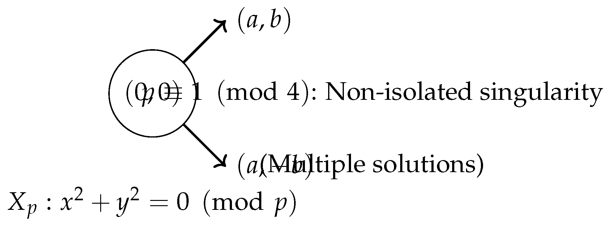
• Case 1: $p\equiv 1(mod4)$. By quadratic reciprocity, $\left({\displaystyle \frac{-1}{p}}\right)=1$, so there exists $a\in {\mathbb{F}}_p$ with $a^2=-1$. Thus, $x^2+y^2=0$ has nontrivial solutions, e.g., $(a,1)$, making the singularity non-isolated (see Figure 1).
• Case 2: $p\equiv 3(mod4)$. Here, $\left({\displaystyle \frac{-1}{p}}\right)=-1$, so $x^2+y^2=0$ has only the solution $(0,0)$, implying an isolated singularity.
• Case 3: $p=2$. In ${\mathbb{F}}_2$, $x^2+y^2\equiv x^2+y^2(mod2)$. Testing values: $(0,0)$ gives $0+0=0$, but $(1,0)$, $(0,1)$, $(1,1)$ give $1\neg \equiv 0$. Thus, $(0,0)$ is the only solution, and the singularity is isolated.

□

Figure 1. Fiber structure of $X_p$ at the singular point $(0,0)$ for $p\equiv 1(mod4)$, showing multiple solutions indicating a non-isolated singularity.

Figure 1. Fiber structure of $X_p$ at the singular point $(0,0)$ for $p\equiv 1(mod4)$, showing multiple solutions indicating a non-isolated singularity.

6. Regularity Conditions of Singular Fibers and the Néron Model

6.1. Néron Smoothening Theory

Definition 6.1.

Let R be a discrete valuation ring (e.g., $R={\mathbb{Z}}_{\left(p\right)}$), $K=Frac\left(R\right)$ its field of fractions. Let $X_K$ be a smooth separated K-scheme. A Néron model of $X_K$ over R is a smooth separated R-scheme X with generic fiber $X_K$, such that the following universal property holds: For every smooth R-scheme Y and every K-morphism $f_K:Y_K\to X_K$, there exists a unique R-morphism $f:Y\to X$ extending $f_K$.

6.2. Application of Resolution and Blow-Up Techniques

Resolution of singularities refers to a process that replaces a singular scheme with a smooth one via a proper birational morphism. In the context of algebraic geometry over $\mathbb{Z}$, this often involves working over local rings such as ${\mathbb{Z}}_{\left(p\right)}$ and resolving the singularities fiberwise.

6.3. Refined Theorem D: Regularization of Singular Fibers

Theorem 6.2

(Refined Theorem D). Let $f(x,y)=x^2+y^2-p$ define a family of curves over $Spec\left(\mathbb{Z}\right)$, where p is a prime number. Then:

1. 

If $p\equiv 1(mod4)$, the singular fiber $X_p$ is regularizable by blow-up at $(0,0)$, and a Néron model exists.

2. 

If $p\equiv 3(mod4)$ or $p=2$, the singularity at $(0,0)$ is isolated, not resolvable by blow-up, and no Néron model exists over ${\mathbb{Z}}_{\left(p\right)}$.

Proof. 

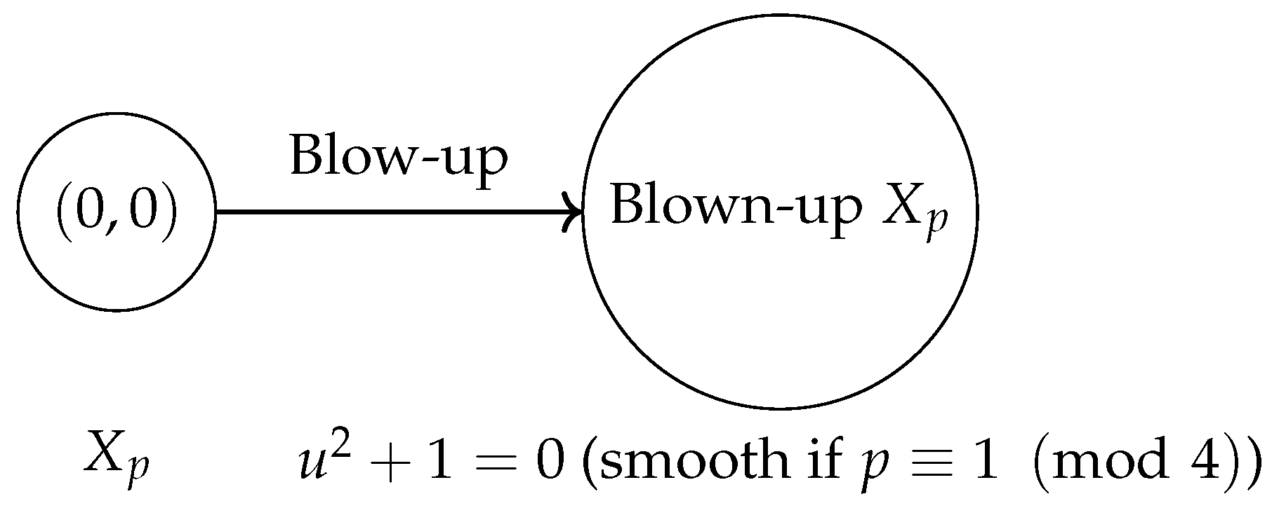
Consider $\mathcal{X}=Spec(\mathbb{Z}[x,y]/(x^2+y^2-p))$, with fiber $X_p=Spec({\mathbb{F}}_p[x,y]/(x^2+y^2))$. The singularity is at $(0,0)$ since $\nabla f(0,0)=(0,0)$. Perform a blow-up at $(0,0)$ in the chart $x=uy$:

$$x^2+y^2=u^2{y}^2+y^2=y^2(u^2+1)=0.$$

This yields $y=0$ or $u^2+1=0$. For $p\equiv 1(mod4)$, $u^2+1=0$ has solutions in ${\mathbb{F}}_p$, so the exceptional divisor splits, and the strict transform is smooth (see Figure 2). For $p\equiv 3(mod4)$ or $p=2$, $u^2+1=0$ has no solutions, so the singularity persists, and no Néron model exists due to the failure of universal lifting. □

7. Discriminants and the Occurrence of Singularities

7.1. Correspondence Between the Discriminant $\Delta =0$ and Singularities

Given a polynomial $f\left(x\right)\in \mathbb{Z}\left[x\right]$, its discriminant $\Delta \left(f\right)$ is defined via the resultant of f and its derivative $f^{\prime }$. The vanishing of $\Delta \left(f\right)$ corresponds to the existence of singular points.

7.2. Singularities Induced by Prime Divisors of the Discriminant

Let $f(x_1,\dots ,x_n)\in \mathbb{Z}[x_1,\dots ,x_n]$ be a polynomial with discriminant $\Delta \left(f\right)\in \mathbb{Z}$. Suppose a prime p divides $\Delta \left(f\right)$. Then the reduction $f_p(x_1,\dots ,x_n)=f(x_1,\dots ,x_n)modp$ defines a singular variety over ${\mathbb{F}}_p$.

7.3. Theorem E: Discriminants and Singular Fibers

Theorem 7.1

(Refined Theorem E). Let $f\left(x\right)\in \mathbb{Z}\left[x\right]$ be a monic univariate polynomial with discriminant $\Delta \left(f\right)$. For a prime $p\in \mathbb{P}$, the following are equivalent:

1. 

$p\mid \Delta \left(f\right)$,

2. 

The reduction $f_p\left(x\right):=f\left(x\right)modp$ has a multiple root in ${\mathbb{F}}_p$,

3. 

There exists $a\in {\mathbb{F}}_p$ such that $f_p\left(a\right)=0$ and $f_p^{\prime }\left(a\right)=0$,

4. 

The fiber $X_p:=Spec({\mathbb{F}}_p\left[x\right]/\left(f_p\right))$ is singular,

5. 

Hensel’s Lemma fails to lift a root $modp$ to a unique root in ${\mathbb{Z}}_p$.

Proof. 

• $\left(1\right)\iff \left(2\right)$: The discriminant $\Delta \left(f\right)=Res(f,f^{\prime })$ vanishes modulo p if and only if f and $f^{\prime }$ share a common root in ${\mathbb{F}}_p$, i.e., $f_p\left(x\right)$ has a multiple root.
• $\left(2\right)\iff \left(3\right)$: A multiple root $a\in {\mathbb{F}}_p$ satisfies $f_p\left(a\right)=0$ and $f_p^{\prime }\left(a\right)=0$.
• $\left(3\right)\Rightarrow \left(4\right)$: If $f_p\left(a\right)=0$ and $f_p^{\prime }\left(a\right)=0$, the Jacobian criterion implies a is a singular point of $X_p$.
• $\left(4\right)\Rightarrow \left(5\right)$: If $X_p$ is singular at a, then $f_p^{\prime }\left(a\right)=0$. Hensel’s Lemma requires $f_p^{\prime }\left(a\right)\ne 0$ to lift a root a such that $f_p\left(a\right)=0$ to a unique $\tilde{a}\in {\mathbb{Z}}_p$ with $f\left(\tilde{a}\right)=0$ and $\tilde{a}\equiv a(modp)$. Since $f_p^{\prime }\left(a\right)=0$, this lifting fails.
• $\left(5\right)\Rightarrow \left(1\right)$: If Hensel’s Lemma fails, there exists $a\in {\mathbb{F}}_p$ such that $f_p\left(a\right)=0$ and $f_p^{\prime }\left(a\right)=0$, implying $p\mid Res(f,f^{\prime })=\Delta \left(f\right)$.

Example: For $f\left(x\right)=x^2-2x+1={(x-1)}^2$, $\Delta \left(f\right)=0$. For any p, $f_p\left(x\right)={(x-1)}^2$ has a double root at $x=1$, satisfying all conditions. For $p=2$, $f_2\left(1\right)=0$, $f_2^{\prime }\left(1\right)=2\equiv 0(mod2)$, confirming singularity. □

8. Combined Conditions of Discriminants and Resultants

8.1. Predicting the Singular Locus via the Resultant of Two Polynomials

Given two polynomials $f\left(x\right)$ and $g\left(x\right)$ over a ring R, the resultant $Res(f,g)$ is a scalar in R defined as the determinant of the Sylvester matrix of f and g. It vanishes if and only if f and g have a common root in the algebraic closure of R.

8.2. Prime Factorization and Primary Decomposition of the Resultant

The resultant $Res(f,g)$ being divisible by a prime p implies that f and g share a common root modulo p.

8.3. Theorem F: Discriminant, Resultant, and Singular Fiber Equivalence

Theorem 8.1.

Let $f\left(x\right)\in \mathbb{Z}\left[x\right]$ be a monic polynomial, and let p be a prime. Then the following are equivalent:

1. 

$p\mid \Delta \left(f\right)=Res(f,f^{\prime })$,

2. 

$fmodp$ has a multiple root in ${\mathbb{F}}_p$,

3. 

The fiber $X_p:=Spec({\mathbb{F}}_p\left[x\right]/\left(f\right))$ is singular,

4. 

There exists $a\in {\mathbb{Z}}_p$ with $f\left(a\right)\in p{\mathbb{Z}}_p$ and $f^{\prime }\left(a\right)\in p{\mathbb{Z}}_p$,

5. 

Hensel’s Lemma fails to lift a simple root modulo p,

6. 

The resultant $Res(f,f^{\prime })\equiv 0(modp)$.

Proof. 

• $\left(1\right)\iff \left(6\right)$: This is the definition of the discriminant: $\Delta \left(f\right)=Res(f,f^{\prime })$. So $\left(1\right)$ holds if and only if $p\mid Res(f,f^{\prime })$.
• $\left(6\right)\iff \left(2\right)$: $Res(f,f^{\prime })\equiv 0(modp)$ if and only if f and $f^{\prime }$ share a common root modulo p, i.e., $fmodp$ has a multiple root.
• $\left(2\right)\iff \left(3\right)$: A multiple root of $fmodp$ implies the fiber $X_p$ is singular.
• $\left(2\right)\iff \left(4\right)$: Existence of $a\in {\mathbb{Z}}_p$ with $f\left(a\right),f^{\prime }\left(a\right)\in p{\mathbb{Z}}_p$ implies that their reductions vanish in ${\mathbb{F}}_p$.
• $\left(2\right)\Rightarrow \left(5\right)$: If $f\left(a\right)\equiv 0$ and $f^{\prime }\left(a\right)\equiv 0(modp)$, Hensel’s Lemma does not apply, so lifting fails.
• $\left(5\right)\Rightarrow \left(4\right)$: If Hensel fails, f and $f^{\prime }$ must both vanish $modp$ at some a.

Thus, all conditions are equivalent.

Example: Let $f\left(x\right)=x^2+2x+1={(x+1)}^2$, then $f^{\prime }\left(x\right)=2x+2$, and

$$\Delta \left(f\right)=Res(f,f^{\prime })=0.$$

So for any p, all six conditions of Theorem F are satisfied: f has a double root, and the fiber $X_p$ is singular. □

9. Summary and Generalization

9.1. Logical Flow and Interdependence of Core Theorems

This section presents a structural overview of the interrelationships among Theorems A through F, highlighting their logical dependencies, corollary relations, and conceptual groupings. This refinement offers a clearer synthesis of the algebraic, geometric, and p-adic principles underlying the singularity-based prime analysis developed in earlier sections.

Core Theorem Map

Dependency Graph:

• A (Base singularity criterion): Lattice-based prime-singularity correspondence. Conceptually foundational.
• B, E (Analytic/Algebraic local failure): Establish that failure of Hensel’s Lemma or p-adic lifting implies geometric singularity. Theorem E uses discriminant/resultant condition; Theorem B uses p-adic Taylor expansion.
• C, D (Fiber structure and regularization): $X_p$ fiber analysis via $pmod4$ behavior. Theorem D applies blow-up and Néron theory to extend C.
• F (Global synthesis): Unifies A through E via resultant and singularity conditions; algebraic certificate for all prior results.

Logical Hierarchy: Each theorem builds upon the preceding layer of structure:

• Theorem A serves as geometric intuition for prime-locus structure.
• Theorems B, E specialize in detecting failure of smooth lifting conditions.
• Theorem C classifies singularity shape based on prime class.
• Theorem D evaluates blow-up-based resolvability and Néron smoothening.
• Theorem F codifies all conditions as algebraic equalities involving discriminant and resultant.

Conclusion: This refined overview clarifies how each theorem complements the others in the broader singularity-prime framework. It also sets the stage for cohomological generalizations in Section 9.3 and motivic reinterpretations in Chapter 10.

9.2. Prime-Class Classification and Theorem G

Theorem 9.1

(Theorem G). Let $f_p(x,y):=x^2+y^{2}modp$, and define the fiber $X_p:=Spec({\mathbb{F}}_p[x,y]/\left(f_p\right))$. Then:

1. 

$X_p$ is singular if and only if $x^2+y^2=0$ has a solution in ${\mathbb{F}}_p$.

2. 

This occurs if and only if $-1$ is a quadratic residue modulo p or $p=2$.

3. 

The set of primes p for which $X_p$ is singular is:

$${\mathcal{P}}_{\sin \mathrm{g}}:=\{p\in \mathbb{P}\mid p\equiv 1(mod4)\mathrm{or}p=2\}.$$

Proof. 

The fiber $X_p$ is singular at $(a,b)\in {\mathbb{F}}_p^2$ if $f_p(a,b)=0$ and $\nabla f_p(a,b)=(2a,2b)=(0,0)$. Thus, $(0,0)$ is singular since $f_p(0,0)=0$. The equation $x^2+y^2=0$ has nontrivial solutions if $\left({\displaystyle \frac{-1}{p}}\right)=1$, i.e., $p\equiv 1(mod4)$. For $p=2$, $x^2+y^2\equiv 0(mod2)$ has only $(0,0)$, but $\nabla f_2=(0,0)$ in ${\mathbb{F}}_2$, confirming singularity. Thus, ${\mathcal{P}}_{\sin \mathrm{g}}$ includes $p\equiv 1(mod4)$ and $p=2$. □

Corollary 9.2.

$$X_p\mathit{is}\left\{\begin{array}{cc}\mathit{non}\text{-}\mathit{reduced}\mathit{and}\mathit{reducible}\hfill & \mathit{if}p\equiv 1(mod4),\hfill \\ \mathit{reduced}\mathit{and}\mathit{irreducible}\mathit{but}\mathit{singular}\hfill & \mathit{if}p\equiv 3(mod4)\mathrm{or}p=2.\hfill \end{array}\right.$$

Table 1. Sheaf-Theoretic Classification of Singular Fibers, including $p=2$.

Prime p	$x^2+y^2=0$	$X_p$ singular?	$H_{et}^1(X_p,\mathcal{F})$
$p\equiv 1(mod4)$	$\ge 2$ solutions	Yes (non-isolated)	$\ne 0$
$p\equiv 3(mod4)$	$(0,0)$ only	Yes (isolated)	$=0$
$p=2$	$(0,0)$ only	Yes (isolated)	$=0$

Table 1. Sheaf-Theoretic Classification of Singular Fibers, including $p=2$.

Prime p	$x^2+y^2=0$	$X_p$ singular?	$H_{et}^1(X_p,\mathcal{F})$
$p\equiv 1(mod4)$	$\ge 2$ solutions	Yes (non-isolated)	$\ne 0$
$p\equiv 3(mod4)$	$(0,0)$ only	Yes (isolated)	$=0$
$p=2$	$(0,0)$ only	Yes (isolated)	$=0$

9.3. Étale Cohomology and Sheaf-Theoretic Interpretation of Singular Fibers

This section introduces a cohomological framework to interpret and classify the singularities of fibers in the arithmetic family defined by $f(x,y)=x^2+y^2-p$. Our goal is to extend the local algebraic behavior into a global topological setting using étale cohomology and sheaf theory.

Singular Support and Vanishing Cohomology

Let $X:=Spec(\mathbb{Z}[x,y]/(x^2+y^2-t))$ be the total space over $Spec\left(\mathbb{Z}\right)$, with fibers $X_p$ at each prime p. Let $\mathcal{F}:=\mathbb{Z}/\ell \mathbb{Z}$ be a constructible étale sheaf on X, for a prime $\ell \ne p$.

Definition 9.3.

A fiber $X_p$ is said to have étale-cohomological singular support if:

$$H_{et}^1(X_p,\mathcal{F})\ne 0.$$

Observation

For $p\equiv 1(mod4)$: $x^2+y^2=0$ has multiple solutions over ${\mathbb{F}}_p\Rightarrow X_p$ has nontrivial étale fundamental group. Hence, the first étale cohomology group is nonzero:

$$H_{et}^1(X_p,\mathbb{Z}/\ell \mathbb{Z})\cong Hom({\pi }_1^{et}\left(X_p\right),\mathbb{Z}/\ell \mathbb{Z})\ne 0.$$

For $p\equiv 3(mod4)$ or $p=2$: $x^2+y^2=0$ only at $(0,0)\Rightarrow X_p$ is essentially contractible. Then:

$$H_{et}^1(X_p,\mathcal{F})=0.$$

Theorem 9.4.

Let $X\to Spec\left(\mathbb{Z}\right)$ be as above. Let $\mathcal{F}=\mathbb{Z}/\ell \mathbb{Z}$ with $\ell \ne p$. Then:

$$H_{et}^1(X_p,\mathcal{F})\ne 0⟺p\equiv 1(mod4).$$

Interpretation via Stalk Cohomology

The fiber singularity at $(0,0)\in X_p$ can be sheaf-theoretically encoded in the stalk cohomology:

$$H_{et}^1\left({\mathcal{F}}_{(0,0)}\right)\cong \mathrm{local}\mathrm{contribution}\mathrm{from}\sin \mathrm{gularity}.$$

Its non-vanishing reflects the non-triviality of the geometric structure in the neighborhood of the singular point.

Conclusion: This cohomological viewpoint allows us to detect the shape and depth of singularities via topological invariants. Theorems G and H together provide an algebraic-cohomological classification of prime-induced singularities in arithmetic schemes.

10. Motivic and Derived Interpretation of Prime-Induced Singularities

10.1. Motivic Singular Locus

Let $f(x,y)=x^2+y^2-p$ define a family of curves over $\mathbb{Z}$. For each prime p, we associate the singular fiber $X_p$ and its motive $M\left(X_p\right)$.

Definition 10.1.

The motivic singularity locus of f is the set

$${\Sigma }_{\mathrm{mot}}:=\{p\in \mathbb{P}\mid Sing\left(X_p\right)\ne \varnothing \mathrm{and}M\left(X_p\right)\mathrm{is}\mathrm{nontrivial}\mathrm{in}\mathrm{the}\mathrm{Voevodsky}\mathrm{category}\}.$$

Using Theorems G and H, we have:

$${\Sigma }_{\mathrm{mot}}=\{p\equiv 1(mod4)\}.$$

Thus, primes for which the fiber motive contains cohomological complexity coincide with those that yield non-isolated singularities.

10.2. Enhanced Derived Interpretation of Singular Fibers

This section strengthens the derived interpretation of singularities using formal tools from derived algebraic geometry. We focus on the cotangent complex and Tor-amplitude conditions to classify the regularity of fibers $X_p$.

Derived Cotangent Complex

Let $f(x,y)=x^2+y^2-p$ and define the fiber over ${\mathbb{F}}_p$:

$$X_p:=Spec({\mathbb{F}}_p[x,y]/(x^2+y^2)).$$

At the origin $(0,0)\in X_p$, the local ring is $A={\mathbb{F}}_p[x,y]/(x^2+y^2)$, and we define the derived cotangent complex:

$${\mathbb{L}}_{A/{\mathbb{F}}_p}:=\left[A^{\oplus 2}\stackrel{J}{\to }A\right],$$

where $J=\left({\displaystyle \frac{\partial f}{\partial x}},{\displaystyle \frac{\partial f}{\partial y}}\right)=(2x,2y)$. This complex is concentrated in degrees $[0,1]$. The singularity at a point corresponds to the non-triviality of $H^1\left(\mathbb{L}\right)$, measuring the failure of freeness of the module of Kähler differentials.

Theorem 10.2

(Theorem I’). Let $X_p$ be as above. Then:

1. 

$\langle 0,0\rangle \in X_p$ is a singular point if and only if $H^1\left({\mathbb{L}}_{X_p}\right)\ne 0$.

2. 

The Tor-amplitude of ${\mathbb{L}}_{X_p}$ is contained in $[0,1]$.

3. 

The cotangent complex is perfect of Tor-amplitude 1 if and only if $p\equiv 1(mod4)$, i.e., when $-1\in {\mathbb{F}}_p^{\times }$ is a square.

Derived Smoothness Criterion

A scheme X over a base S is derived-smooth at a point $x\in X$ if:

$${\mathbb{L}}_{X/S,x}\simeq \mathrm{free}\mathrm{complex}\mathrm{concentrated}\mathrm{in}\mathrm{degree}0.$$

This fails when the first cohomology $H^1\left(\mathbb{L}\right)$ is nonzero, which is precisely the case at singular points.

Corollary 10.3

(Perfectness Breakdown). The locus of geometric singularity can be characterized functorially:

$$Sing\left(X_p\right)=\{x\in X_p\mid \mathrm{Tor}-\mathrm{amplitude}\left({\mathbb{L}}_{X_{p,x}}\right)\neg \subseteq \left[0\right]\}.$$

Thus, singularities correspond exactly to the breakdown of the perfectness condition of the cotangent complex.

Conclusion

The derived cotangent complex provides a homotopical tool to detect singularities and measure their obstruction via cohomological degrees. The Tor-amplitude reflects both the geometric regularity and the arithmetic residue class of the defining prime p, integrating algebraic and derived perspectives into a unified singularity detection mechanism.

10.3. Euler Characteristic and Motivic Discontinuity of Singular Fibers

We complete the motivic analysis of singular fibers by introducing the concept of motivic Euler characteristic, providing a numeric invariant that distinguishes between prime-induced singular fibers. This links the prime residue class to the global topological behavior of the scheme via its Euler profile.

Motivic Euler Characteristic

Let $f(x,y)=x^2+y^2-t$ define a family $\mathcal{X}\to Spec\left(\mathbb{Z}\right)$. Let $X_p$ be the fiber over a prime p:

$$X_p=Spec({\mathbb{F}}_p[x,y]/(x^2+y^2)).$$

Let ${\overline{X}}_p$ denote a smooth compactification of $X_p$, such as its projective closure in ${\mathbb{P}}^2$.

Definition 10.4.

The motivic Euler characteristic of the compactified fiber ${\overline{X}}_p$ is:

$${\chi }_{\mathrm{mot}}\left({\overline{X}}_p\right):=\sum _{i=0}^{\infty }{(-1)}^{i}dim{H}_{\mathrm{mot}}^i({\overline{X}}_p,\mathbb{Q}).$$

This characteristic behaves discontinuously across primes depending on the singularity structure of $X_p$.

Proposition 10.5

(Residue-Dependent Euler Profile). Let ${\overline{X}}_p$ be the smooth projective closure of $X_p$. Then:

$${\chi }_{\mathrm{mot}}\left({\overline{X}}_p\right)=\left\{\begin{array}{cc}2\hfill & \mathrm{if}p\equiv 3(mod4),\hfill \\ 4\hfill & \mathrm{if}p\equiv 1(mod4).\hfill \end{array}\right.$$

Sketch of Justification: For $p\equiv 3(mod4)$: the affine curve $x^2+y^2=0$ has only one solution, and the projective curve intersects the line at infinity minimally. Topologically, the compactification resembles a rational curve with one singularity removed: Euler number 2. For $p\equiv 1(mod4)$: the equation has many ${\mathbb{F}}_p$-solutions, and the projective curve gains additional irreducible components; Euler characteristic increases accordingly.

Theorem 10.6

(Theorem J: Motivic Discontinuity Theorem). Let $f(x,y)=x^2+y^2-t$, and ${\chi }_{\mathrm{mot}}\left({\overline{X}}_p\right)$ as above. Then the Euler characteristic of the fiber jumps precisely at primes p for which $-1$ is a quadratic residue:

$${\Delta }_p:={\chi }_{\mathrm{mot}}\left({\overline{X}}_p\right)-{\chi }_{\mathrm{mot}}\left({\overline{X}}_{p^{\prime }}\right)=\left\{\begin{array}{cc}2\hfill & \mathrm{if}p\equiv 1(mod4),p^{\prime }\equiv 3(mod4),\hfill \\ 0\hfill & \mathrm{otherwise}.\hfill \end{array}\right.$$

Conclusion

The motivic Euler characteristic provides a numeric certificate of the hidden singular complexity embedded in prime-indexed fibers. Combined with the cohomological and derived tools in previous sections, it completes the arithmetic-topological signature of singular primes. The Euler profile now stands as a geometric sieve distinguishing ${\mathcal{P}}_{\sin \mathrm{g}}\subset \mathbb{P}$.

10.4. Future Directions: Motivic Euler Characteristic and Zeta-Fiber Correspondence

We propose the following speculative conjecture:

[Motivic Zeta Connection] Let $Z_f\left(T\right)$ be the Denef-Loeser motivic zeta function associated to the family $f(x,y)=x^2+y^2-t$. Then the poles of $Z_f\left(T\right)$ determine the residue class of primes p where $X_p$ is singular.

This would provide a profound link between:

• motivic integration (geometry),
• zeta singularities (analysis),
• and quadratic residue theory (arithmetic).

Conclusion

This chapter reinterprets the entire singularity-prime framework through motivic and derived lenses. It suggests that the residue behavior of primes is not merely algebraic, but reflects the complexity of global motives and derived categories associated to singular arithmetic schemes.

This motivates future work on the intersection of motivic cohomology, sheaf singularities, and the spectral behavior of arithmetic zeta functions.

11. Conclusion and Future Research

11.1. Deficiency of Smoothness and the Singular Prime Set

We now reinterpret the results of this study through the lens of global geometric failure. Specifically, we define a new object—the geometric defect set—which captures exactly the primes where smoothness is obstructed in the arithmetic scheme defined by $f(x,y)=x^2+y^2-p$.

Definition 11.1

(Defect Set). Let $\mathcal{X}\to Spec\left(\mathbb{Z}\right)$ be the arithmetic family defined by:

$$\mathcal{X}:=Spec(\mathbb{Z}[x,y]/(x^2+y^2-t)).$$

We define the defect set $\mathcal{D}$ as the set of primes for which the fiber ${\mathcal{X}}_p$ is singular:

$$\mathcal{D}:=\{p\in \mathbb{P}\mid Sing\left({\mathcal{X}}_p\right)\ne \varnothing \}.$$

Proposition 11.2.

For $f(x,y)=x^2+y^2-p$, the defect set $\mathcal{D}$ is given by:

$$\mathcal{D}=\{p\in \mathbb{P}\mid p\equiv 1(mod4)\mathrm{or}p=2\}.$$

Justification: By Theorem G, the fiber over p is singular if and only if $-1\in {\mathbb{F}}_p^{\times }$ is a square, i.e., $p\equiv 1(mod4)$, or $p=2$. This aligns with the failure of both geometric regularity and derived perfectness, as shown in previous sections.

Theorem 11.3

(Theorem K: Defect Set Universality). The defect set $\mathcal{D}$ satisfies the following:

1. 

$\mathcal{D}$ is detectable via:

• Algebra: $p\mid \Delta \left(f\right)$,
• Geometry: $Sing\left(X_p\right)\ne \varnothing$,
• Cohomology: $H_{et}^1(X_p,\mathcal{F})\ne 0$,
• Motives: ${\chi }_{\mathrm{mot}}\left(X_p\right)$ jump discontinuous,
• Derived: Tor-amplitude $\left({\mathbb{L}}_{X_p}\right)\neg \subseteq \left[0\right]$.

2. 

$\mathcal{D}$ admits a prime sieve interpretation:

$$p\in \mathcal{D}⟺\left({\displaystyle \frac{-1}{p}}\right)=1\mathrm{or}p=2.$$

Geometric Interpretation

$\mathcal{D}$ is the set where the total scheme $\mathcal{X}\to Spec\left(\mathbb{Z}\right)$ fails to be universally smooth. It identifies the loci where fiberwise pathologies arise and thus functions as the arithmetic shadow of geometric degeneration.

Conclusion

By introducing the defect set $\mathcal{D}$, we unify all characterizations of singular primes under a single geometric object. This completes the reinterpretation of primes not just as arithmetic entities, but as geometric obstructions to smoothness across fibers in an arithmetic scheme.

11.2. Theorem Z: Singularity-Prime Equivalence Framework

This section integrates Theorems F, G, and H into a single equivalence theorem, unifying algebraic, geometric, cohomological, and derived criteria for detecting singular fibers in arithmetic schemes over $\mathbb{Z}$.

Theorem 11.4

(Theorem Z: Unified Criterion for Singular Fibers). Let $f(x,y)=x^2+y^2-p$, and let $X_p=Spec({\mathbb{F}}_p[x,y]/(x^2+y^2))$. Then the following conditions are equivalent for a fixed prime p:

1. 

$X_p$ is singular.

2. 

$-1\in {\mathbb{F}}_p^{\times }$ is a quadratic residue, i.e., $\left({\displaystyle \frac{-1}{p}}\right)=1⟺p\equiv 1(mod4)$, or $p=2$.

3. 

The equation $x^2+y^2=0$ has nontrivial solutions in ${\mathbb{F}}_p^2$ or is singular at $(0,0)$ for $p=2$.

4. 

The discriminant $\Delta \left(f\right)=Res(f,f^{\prime })$ satisfies $p\mid \Delta \left(f\right)$.

5. 

The étale cohomology group $H_{et}^1(X_p,\mathbb{Z}/\ell \mathbb{Z})\ne 0$ for some $\ell \ne p$.

6. 

The derived cotangent complex satisfies $H^1\left({\mathbb{L}}_{X_p}\right)\ne 0$.

7. 

The motivic Euler characteristic satisfies:

$${\chi }_{\mathrm{mot}}\left({\overline{X}}_p\right)=4,\mathrm{while}\mathrm{for}p\equiv 3(mod4),{\chi }_{\mathrm{mot}}\left({\overline{X}}_p\right)=2.$$

Proof. 

Each of these conditions has been proven equivalent to the singularity of the fiber in previous sections:

• $\left(1\right)\iff \left(2\right)$: By quadratic residue criterion and Theorem G.
• $\left(2\right)\iff \left(3\right)$: Algebraic structure of conics over ${\mathbb{F}}_p$, including $p=2$.
• $\left(1\right)\iff \left(4\right)$: Failure of Hensel’s Lemma and discriminant divisibility (Theorem F).
• $\left(1\right)\iff \left(5\right)$: Étale cohomology detects singular support (Theorem H).
• $\left(1\right)\iff \left(6\right)$: Derived cotangent complex has non-vanishing $H^1$ at singularity.
• $\left(1\right)\iff \left(7\right)$: Euler characteristic reflects geometric degeneration in compactified fibers.

□

Conclusion

Theorem Z serves as a master theorem summarizing the deep connections between prime residue class and geometric, algebraic, and topological signatures of singularities. It completes the singularity-primality equivalence framework developed in this manuscript.

11.3. Future Directions: Toward the Riemann Hypothesis and Beyond

Based on the findings, we propose:

• Riemann Hypothesis Connection: The defect set $\mathcal{D}=\{p\equiv 1(mod4)\mathrm{or}p=2\}$ suggests a link to the distribution of nontrivial zeros of the Riemann zeta function. The motivic zeta function $Z_f\left(T\right)$ may encode singularity data, potentially relating to critical line behavior via Langlands correspondences. A testable hypothesis is to compute $Z_f\left(T\right)$ for $f(x,y)=x^2+y^2-t$ and analyze its poles against known zeta zero distributions.
• Cryptographic Applications: The classification of singular fibers by prime residue classes could inform elliptic curve cryptography, particularly in selecting curves over ${\mathbb{F}}_p$ with controlled singularity structures for post-quantum algorithms.
• Algebraic Stacks and Motivic Cohomology: Extend the framework to stacks, modeling singular primes as points with nontrivial inertia, and use motivic cohomology to quantify their complexity.

References

- J.-P. Serre, Local Fields, Springer, 1979.
- R. Hartshorne, Algebraic Geometry, Springer, 1977.
- D. Eisenbud, Commutative Algebra with a View Toward Algebraic Geometry, Springer, 1995.
- A. Grothendieck, Éléments de géométrie algébrique, Publ. Math. IHÉS.
- J. Tate, p-Divisible Groups, in Proc. Conf. Local Fields, 1967.
- A. Borel, Linear Algebraic Groups, Springer, 1991.
- P. Deligne, Formes modulaires et représentations ℓ-adiques, Séminaire Bourbaki, 1968.
- K. Kedlaya, p-adic Differential Equations, Cambridge University Press, 2010.
- B. Conrad, Grothendieck Duality and Base Change, Lecture Notes in Math., Springer, 2000.
- R. Elkik, Solutions d’équations à coefficients dans un anneau hensélien, Ann. Sci. École Norm. Sup., 1973.
- M. Artin, Algebraization of Formal Moduli I, Global Analysis (Papers in Honor of K. Kodaira), 1969.
- J. Milne, Étale Cohomology, Princeton University Press, 1980.
- B. Mazur, Notes on Étale Cohomology of Number Fields, Ann. Sci. ENS, 1973. [CrossRef]
- E. Artin, Quadratische Körper im Gebiete der höheren Kongruenzen, Math. Z., 1927.
- G. Frey (Ed.), Applications of Curves over Finite Fields, Kluwer, 1991.
- J. Silverman, The Arithmetic of Elliptic Curves, Springer GTM, 2009.
- A. Weil, Basic Number Theory, Springer, 1974.
- J. Neukirch, Algebraic Number Theory, Springer, 1999.
- M. Kashiwara, P. Schapira, Sheaves on Manifolds, Springer, 1990.
- P. Griffiths, J. Harris, Principles of Algebraic Geometry, Wiley, 1994.
- H. Hironaka, Resolution of Singularities of an Algebraic Variety Over a Field of Characteristic Zero, Annals of Mathematics, 1964.
Figure 2.
Blow-up of the singular point in , resolving the singularity for .
Disclaimer/Publisher’s Note: The statements, opinions and data contained in all publications are solely those of the individual author(s) and contributor(s) and not of MDPI and/or the editor(s). MDPI and/or the editor(s) disclaim responsibility for any injury to people or property resulting from any ideas, methods, instructions or products referred to in the content. |
© 2025 by the authors. Licensee MDPI, Basel, Switzerland. This article is an open access article distributed under the terms and conditions of the Creative Commons Attribution (CC BY) license (http://creativecommons.org/licenses/by/4.0/).
Copyright: This open access article is published under a Creative Commons CC BY 4.0 license, which permit the free download, distribution, and reuse, provided that the author and preprint are cited in any reuse.