Submitted:
25 June 2025
Posted:
26 June 2025
You are already at the latest version
Abstract
Soil moisture is a key parameter in agriculture. Its accurate prediction is essential for effective irrigation scheduling and water use efficiency. This study introduces a hybrid approach integrating Long Short-Term Memory (LSTM) network and Extreme Gradient Boosting (XGBoost) model for multistep soil moisture prediction for (24 hours, 72 hours, and 168 hours) ahead. The LSTM captures temporal dependencies and extracts high-level features from the dataset, while XGBoost uses these features to make final predictions. The proposed method was trained and evaluated on a real-world data from the D.A.T.A (Demonstrating Applied Technology in Agriculture) research farm at ABAC (Abraham Baldwin Agricultural College) Tifton, GA, USA, utilizing watermark soil moisture sensors and weather station’s data installed in the farm. Experimental results show that, the pro-posed method outperforms standalone models like LSTM, XGBoost, Gradient Boosting (GB), Extra Trees (ET) and others. It achieved R² values of 0.9867, 0.9854, and 0.9856 for 24, 72 and 168-hour predictions respectively. These results demonstrate the effectiveness of LSTM in extracting high-level temporal features, and XGBoost in making final predictions. The proposed hybrid model offers precise soil moisture prediction, making it a practical tool for real-time irrigation scheduling and enhancing water use efficiency in precision agriculture.
Keywords:
long short-term memory
; ensemble learning
; iot sensors
; artificial intelligence
; deep learning
; machine learning
; autonomous irrigation
; soil moisture
1. Introduction
1.1. Background and Motivation
Soil moisture, a critical parameter in agricultural practices, significantly influences crop growth, irrigation management, and climate modeling. Soil moisture levels can be measured by in-place probes or remote sensing techniques [1] and can fluctuate due to several factors, including evaporation, precipitation, transpiration, and irrigation. The amount of water present in the soil affects root water uptake, soil aeration, and microbial activity, directly impacting crop productivity [2]. Accurate soil moisture predictions are essential for optimizing irrigation schedules, reducing water wastage, and ensuring sustainable farming practices, particularly in water-scarce regions. In addition to its agricultural significance, soil moisture is fundamental to understanding the Earth’s hydrological cycle, meteorological processes, and climatic patterns [3,4]. It influences a wide range of activities, from crop yield prediction and irrigation scheduling to extreme weather forecasting and climate change studies.
Traditional soil moisture prediction methods, including empirical formulas, models based on soil water balance, and statistical approaches such as autoregressive integrated moving average (ARIMA) models, have been widely used [5,6]. However, these methods often fall short in handling the complex and dynamic relationships between soil moisture and environmental variables. Empirical formulas are simplistic and often inaccurate, while models based on soil water dynamics or water balance require site-specific data and can be computationally intensive. Statistical approaches, such as ARIMA, are limited by their inability to capture long-term dependencies and non-linear relationships [7]. To overcome these limitations, machine learning (ML) and deep learning (DL) models have emerged as powerful alternatives especially due to their ability to predict soil moisture levels with high accuracy and precision [8,9,10,11,12,13,14,15,16,17].
Traditional standalone ML models have shown promising results in predicting soil moisture for single-step forecasts, typically for short-term predictions (e.g., next few hours). However, when tasked with predicting soil moisture over longer periods, these models tend to struggle, especially when capturing the temporal dependencies and complex relationships between weather variables and soil moisture dynamics. The inability of traditional standalone ML models to generalize effectively over multistep predictions has been a major limitation in precision agriculture, where real-time predictions are crucial for making timely irrigation decisions. In contrast, DL models, particularly Long Short-Term Memory (LSTM) networks and variants like Bi-directional LSTMs (Bi-LSTM), have been shown to outperform traditional models in capturing the temporal dependencies in time-series data [5,18,19]. LSTM models are designed to handle sequential data and are effective at learning patterns over longer periods, making them suitable for multistep ahead predictions. However, while standalone models like LSTM are effective at extracting features from sequential data, they may benefit from the integration of additional ML models for final prediction.
The motivation behind this study is to improve soil moisture prediction accuracy over multiple time steps, focusing on 24-hour, 72-hour, and 168-hour prediction. By comparing standalone ML and DL models with hybrid models that combine the strengths of both DL and ML approaches, the study aims to assess the effectiveness of these models for multi-step predictions. This research aims to provide insights into the strengths and weaknesses of traditional ML and DL models, contributing to the development of more accurate and reliable tools for precision agriculture.
In particular, this study proposes a hybrid approach that combines LSTM with XGBoost. This hybrid model (LSTM + XGBoost) enhances the performance of multistep soil moisture predictions by leveraging LSTM’s ability to capture long-term spatial-temporal dependencies in the data, while XGBoost excels at handling complex, non-linear relationships to make accurate final predictions. By integrating both methods, we create a robust and effective model that can predict soil moisture for the next 24, 72 and 168 hours, effectively using historical soil moisture and weather data. The primary goal of this study is to improve irrigation scheduling optimization and water-use efficiency. The performance of the proposed hybrid model will be compared against several standalone ML/DL models, including Gradient Boosting (GB), Support Vector Machines (SVM), Extreme Gradient Boosting (XGBoost), Random Forest (RF), Ridge Regression (RR), Extra Trees (ET), AdaBoost, K-Nearest Neighbors (KNN), Decision Tree (DT), Multi-Layer Perceptron (MLP), Linear Regression (LR), ElasticNet, Convolutional Neural Networks (CNN), Recurrent Neural Networks (RNN), and Gated Recurrent Units (GRU) along with other hybrid methods.
1.2. Literature Review
1.2.1. LSTM methods for soil moisture prediction
LSTM models have been extensively utilized for soil moisture prediction due to their ability to capture long-term temporal dependencies. A study by [7] proposed an attention-aware LSTM model (ILSTM_Soil) for multistep soil moisture and temperature predictions, demonstrating strong performance with an R² of 0.9580 and an RMSE of 1.033 for 7-day predictions. This model outperformed traditional machine learning methods, including Elastic-Net, RF, SVR, and standard LSTM, effectively capturing the underlying patterns in soil moisture and temperature. In another study, [20] applied LSTM for short-term soil moisture predictions (1 to 24 hours), achieving an impressive R² of 0.98 for 1-hour forecasts, although accuracy declined as the prediction horizon increased, highlighting LSTM’s effectiveness for short-term forecasting and its limitations for long-term predictions.
A study [21] further explored LSTM’s potential for multistep prediction, using meteorological parameters such as air temperature, precipitation, and vapor pressure deficit to forecast volumetric soil moisture up to three days ahead in Serbia. The LSTM model outperformed both RF (MASE = 1.42, MAE = 0.021) and ARIMA (MASE = 2.85, MAE = 0.055), demonstrating its strong generalization capabilities and making it a promising tool for digital irrigation scheduling in diverse climatic conditions. In a greenhouse setting in Chiang Mai, Thailand, another study [22] found that LSTM outperformed Bi-LSTM, with an RMSE of 0.72 compared to 0.76, confirming LSTM’s effectiveness in improving irrigation scheduling. Additionally, the integration of LSTM with IoT-based systems in citrus orchards [23] demonstrated that the Bi-LSTM model (R² = 0.977) outperformed Multi-Layer Neural Networks (MLNN, R² = 0.865), effectively optimizing irrigation and fertilization management.
Lastly, a study in [15] introduced a multi-head LSTM model designed to enhance soil moisture prediction over different time frames. By processing data at various temporal scales and combining the outputs through weighted averaging, the multi-head LSTM model achieved a high R² of 95.04%, demonstrating its potential for accurate long-term soil moisture forecasting.
1.2.2. Hybrid LSTM models for soil moisture prediction
Hybrid models combining LSTM with other machine learning (ML) and deep learning (DL) techniques have shown significant improvements in soil moisture prediction accuracy. In a 2023 study [24], a Conv-LSTM model, which integrates Convolutional Neural Networks (CNN) with LSTM layers, was proposed to enhance spatial-temporal soil moisture predictions, particularly in regions with pronounced seasonal effects. The Conv-LSTM model achieved an R² of 0.92, demonstrating its potential for spatial-temporal predictions in agricultural applications. Additionally, the study highlighted the use of AI-based methods, such as permutation importance, for model interpretability, further solidifying the model’s applicability in precision agriculture.
A novel encoder-decoder LSTM model with residual learning (EDT-LSTM) was introduced in 2023 [25] to improve prediction accuracy by incorporating intermediate time-series data. Tested on FLUXNET site data, the model showed significant improvements in R², ranging from 7.95% for 1-day predictions to 19.71% for 10-day forecasts. This study underscores the potential of encoder-decoder models to enhance soil moisture forecasting in diverse agricultural settings, providing valuable insights for real-time irrigation management. In 2024, a hybrid particle swarm optimization (PSO) and LSTM model (PSO-LSTM) was proposed [13] to predict soil moisture at varying depths using Sentinel-1A satellite data. The model, tested with five input combinations based on vertical (VV) and cross (VH) polarization data, outperformed standalone LSTM by achieving a significantly lower normalized root mean square error (NRMSE) of 4.568–11.023%, compared to 18.056–30.156% for standalone LSTM. The PSO-LSTM model performed best using only VV polarization input, making it a highly effective approach for large-scale precision irrigation management. Another 2024 study [3] explored hybrid LSTM models, including feature attention-based LSTM (FA-LSTM) and generative adversarial network-based LSTM (GAN-LSTM), to further improve soil moisture prediction accuracy. Results showed that LSTM, combined with feature-attention mechanisms, outperformed CNN and transformer models, achieving R² values of 0.943 for 1-day predictions and 0.816 for 7-day predictions. These findings emphasize the promising potential of hybrid LSTM approaches for more accurate soil moisture predictions across diverse soil types and depths, offering substantial improvements over standalone models.
1.2.3. Classical ML/DL methods for soil moisture prediction
Classical ML and DL methods have been widely used to enhance the accuracy and efficiency of soil moisture prediction, especially for multistep forecasting. A study in 2023 [6] proposed a stacked ML method that integrates multiple algorithms (MLP, RF, and SVR) for multistep soil moisture prediction. The study used two input sets: Model A included meteorological factors like precipitation, temperature, humidity, and wind speed, while Model B focused solely on precipitation data. The stacked model outperformed individual models, achieving an R² of 0.962, surpassing MLP (R² = 0.957), RF (R² = 0.956), and SVR (R² = 0.951). This approach highlights how stacking ML models can mitigate individual model weaknesses and improve soil moisture estimation accuracy. Another study [9] utilized LightGBM for soil moisture prediction using high-resolution IoT sensor data from Brazilian farmlands. The model outperformed several other methods, including LR, DT, RF, MLP, LSTM, and Spectral Temporal GraphNN (StemGNN), with an R² of 0.98, MAE of 0.24, and RMSE of 0.48. The study emphasized the importance of incorporating context-aware indices such as past soil moisture and precipitation forecasts, demonstrating significant improvements in prediction accuracy for irrigation scheduling.
In 2021, a Deep Neural Network Regression (DNNR) model [11] was proposed for soil moisture prediction using data from three distinct locations. The model achieved an R² of 0.98 at the Yanqing site, highlighting the potential of deep learning methods to enhance the generalization ability of soil moisture models, thus enabling more accurate predictions across diverse climatic conditions. A 2020 study [26] introduced a Modified Flower Pollination Algorithm (MFPA) combined with Artificial Neural Networks (ANN), referred to as NN-MFPA, for soil moisture prediction. The model was compared with Particle Swarm Optimization (PSO)-ANN, Cuckoo Search (CS)-ANN, and MLP-FFN classifiers, with NN-MFPA achieving the lowest RMSE of 0.0019, outperforming other models. The method’s effectiveness was validated using the Wilcoxon rank test at a 5% significance level, proving its superiority for soil moisture prediction under varying weather conditions and making it suitable for sustainable agriculture and socio-economic stability.
In 2021, another study [27] used soil temperature as a predictor for soil moisture content. The study compared various methods including Multivariate Adaptive Regression Splines (MARS), RF, M5-Tree, MLR, and MLP. Initial models using only soil temperature showed low accuracy, but when incorporating periodicity factors such as year, month, day, and hour, prediction accuracy significantly improved. The study showed that MARS (R = 0.967, d = 0.983) and RF (R = 0.965, d = 0.981) performed best, with MLR consistently underperforming (R = 0.580, d = 0.488). These findings suggest that integrating periodicity with soil temperature improves soil moisture prediction, making it a robust solution for traditional estimation methods.
1.3. Contributions of the study
This study proposes a novel hybrid approach combining LSTM with XGBoost for multistep ahead soil moisture prediction, targeting the next 24 hours, 72 hours, and 168 hours. The LSTM captures long-term spatial-temporal dependencies in the data, while XGBoost handles complex, non-linear relationships, resulting in a more accurate and reliable prediction model. This approach contributes to the optimization of irrigation scheduling and the improvement of water-use efficiency by leveraging historical soil moisture and weather data. In addition, this research offers an in-depth performance comparison of the proposed hybrid model against several standalone and hybrid ML and DL models. It provides insights into the strengths and limitations of different approaches for multistep ahead soil moisture prediction. Overall, this study establishes a benchmark for soil moisture prediction, particularly in using lag-based soil moisture and weather data, contributing to more efficient irrigation practices and sustainable agricultural management.
1.4. Objectives of the Study
The primary objective of this study is to develop and evaluate a hybrid deep learning and machine learning model for multistep soil moisture prediction. Specifically, the study aims to:
1. Develop a hybrid LSTM + XGBoost model to predict soil moisture at 24-hour, 72-hour, and 168-hour intervals using historical soil moisture and weather data.
2. Evaluate the performance of the proposed hybrid model against standalone ML and DL models, including LSTM, XGBoost, GB, RF, and others.
3. Assess the ability of LSTM to capture long-term temporal dependencies in time-series soil moisture and meteorological data for improved feature representation.
4. Investigate the role of XGBoost in refining predictions by leveraging non-linear relationships within LSTM-extracted features.
2. Materials and Methods
2.1. Dataset description
The dataset used for this research was collected from March to December 2024, as part of the University of Georgia’s 4D farm (Digital and Data-Driven Demonstration Farm) on the Abraham Baldwins Agricultural College (ABAC) D.A.T.A. (Demonstrating Applied Technology in Agriculture) farm, located in Tifton, Georgia, USA (GPS coordinates: 31.485043, –83.543575). IoT device sensors were installed in the farm to measure soil moisture content and weather condition in the fields as shown in Table 1.
The farm is divided into four (4) fields namely; Front Field, North Pivot, South Pivot and West Field with a total of fourteen (14) watermark soil moisture sensors (Realm5 Inc.) named 4D 01 to 4D 14. The Front Field contains two soil moisture sensors (4D 01 and 4D 02) while the rest contain four sensors each; North Pivot (4D 03 – 4D 06), South Pivot (4D 07 - 4D 10) and West Field has (4D 11 – 4D 14).
This study focuses exclusively on the South Pivot field. For each timestamp, the soil moisture value used in the analysis was calculated as the average of the four active sensors located in that field. Each soil moisture device records soil moisture and temperature at three depths: 8 inches, 16 inches, and 24 inches, measured in kilopascals (kPa) and Celsius (C), respectively. A single on-site weather station records the following atmospheric parameters: air temperature, dew point, humidity, solar radiation, rainfall, wind speed, wind direction, wind gust, and air pressure.
2.2. Data acquisition and preprocessing
Firstly, we access the soil moisture and weather measurements from two separate web API endpoints via python requests. These measurements are recorded at different time intervals (weather data recorded every 15 minutes, soil moisture recorded every hour) and are merged together into a CSV datasheet. (Merged feature distribution is shown in Figure 2). Figure 1 shows the data acquisition and pre-processing pipeline, generating the final dataset for model training and testing. Since weather readings are measured and recorded in 15 min. intervals and soil moisture is recorded every hour, there are four instances of weather readings for each instance of soil moisture reading, hence these data were merged based on their timestamps.
Initially, the timestamp column was converted into a datetime object to ensure proper handling of time-dependent data. To capture temporal dependencies in soil moisture, lagged features are created for average moisture readings using different time intervals (LSTM window), including 1, 6, 12, 24, 48, and 96 hour historical readings These lagged features help the model understand the influence of past moisture measurements on current and future soil moisture levels.
Missing values in the dataset are addressed by removing any rows with incomplete data, ensuring that only valid, clean data is used for model training. The data is then normalized using the MinMaxScaler, which scales the features to a range between 0 and 1, improving the convergence speed of the machine learning models and ensuring that no feature dominates due to its scale. Data is split into 60% training, 20% validation and 20% testing.
Figure 1.
Data acquisition and processing workflow.
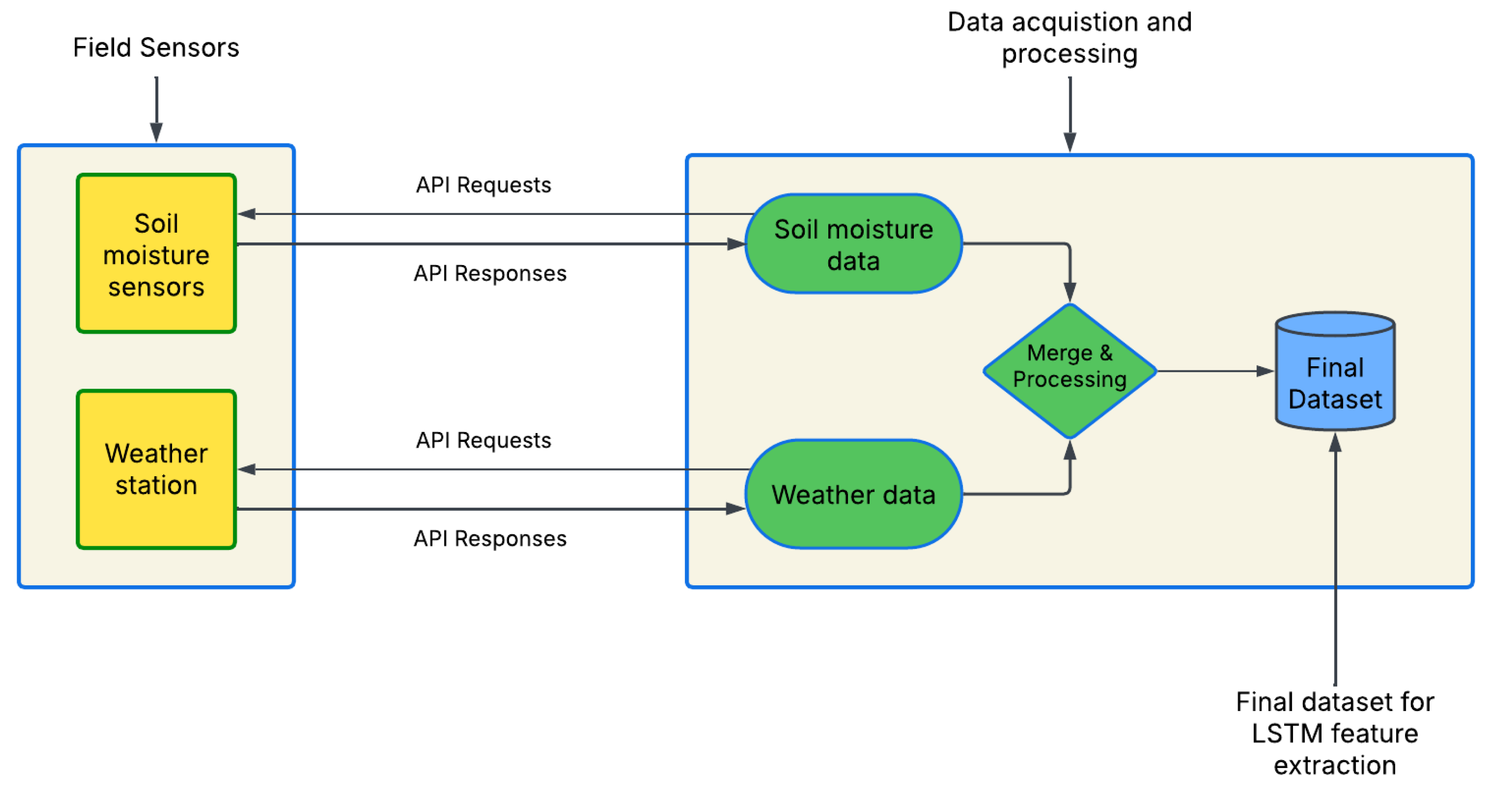
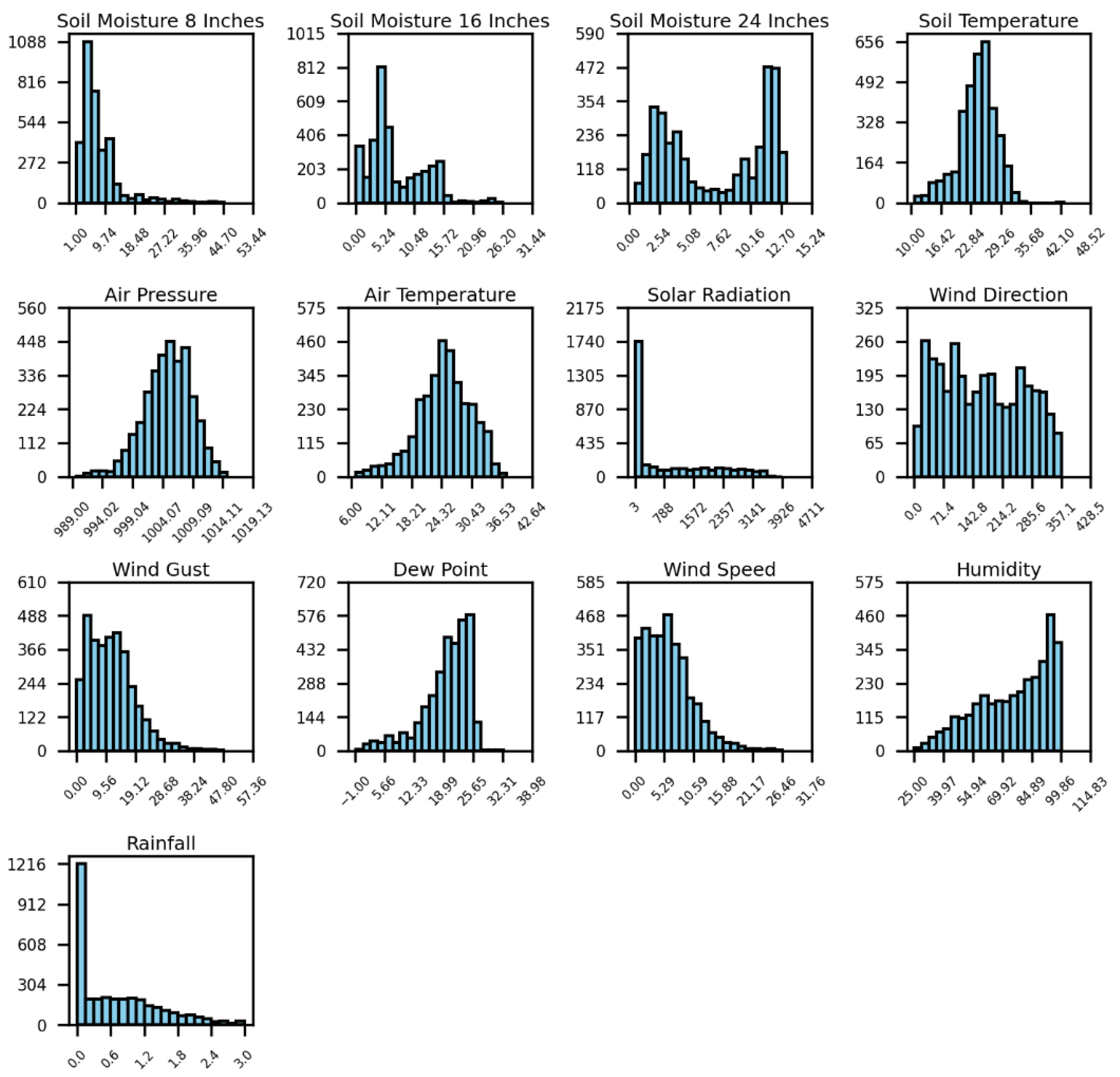
Figure 2 presents a visual representation of the feature frequencies for ten months (March 2024 to December 2024) in the South Pivot field. After merging the weather and soil moisture data, soil moisture is recorded at three depths—8, 16, and 24 inches—where the average value is used as the target variable for prediction. Soil temperature, measured by the IoT sensor device, is another parameter considered. The remaining features, including air temperature, air pressure (Pa), solar radiation (W/m2), wind direction (degrees), wind gust (kph), wind speed (kph), humidity (%), dew point temperature (C), and rainfall (in.), are measured by the weather station sensors.
Figure 1.
Feature distribution for model inputs during 2024 in the South Pivot field.
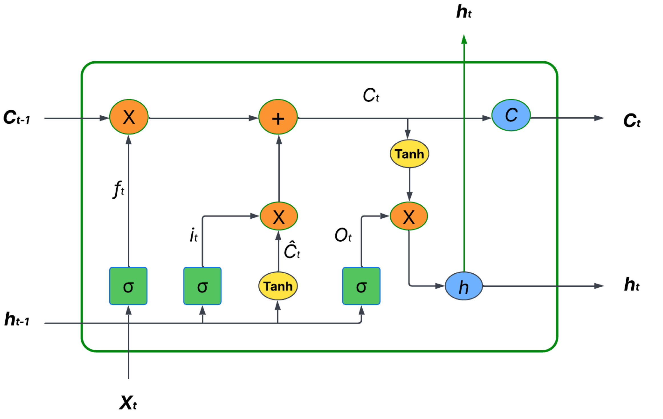
2.3. General LSTM architecture
An LSTM is a neural network derived from recurrent neural networks (RNN), designed to overcome vanishing and exploding gradient issues in time-series forecasting. They contain memory cells that store long-term dependencies, making them particularly effective for soil moisture prediction, where past moisture conditions influence future values. A standard LSTM unit consists of an input gate to update the cell state with new information, a forget gate which decides what information from previous states should be dropped and the output gate to determines the final output based on the cell state. Figure 3 represents a general LSTM architecture.
Figure 2.
General LSTM architecture with input gate, forget gate and output gate [28].
Figure 2.
General LSTM architecture with input gate, forget gate and output gate [28].
The standard LSTM block is presented by equations (1) to (6):
The input gate, denoted as it , determines which new information from the current input xt and the previous hidden state ht−1 should be added to the cell state. Its activation is calculated using the sigmoid function σ, applied to a weighted sum of the concatenated input and previous hidden state [ht−1, xt], along with its associated weight matrix Wi and bias bi. Similarly, the forget gate denoted as ft, decides what information to discard from the cell state based on its own weight matrix Wf, bias bf, and sigmoid activation σ. The output gate, Ot, controls what information from the current cell state will be output as the hidden state ht. It also uses the sigmoid function σ applied to a weighted combination of [ht−1, xt] with its weight matrix Wo and bias bo. The symbol ⊙ represents element-wise multiplication, a crucial operation within the LSTM to selectively filter and combine information. The hyperbolic tangent function tanh, is used to produce outputs in the range of (-1 to 1) often applied to the cell state when calculating the candidate values or the final hidden state.
2.4. Proposed LSTM architecture
The proposed LSTM model architecture consists of three sequential LSTM layers followed by a dropout layer and two fully connected (dense) layers, as summarized in Table 2. The input to the model is a 24-hour time series, where 24 represents the number of time steps, and 32 denotes the batch size as shown in Table 2. The first LSTM layer outputs a sequence of 256 features for each time step, which is passed to the second LSTM layer that reduces it to 128 features per time step. The third LSTM layer outputs only the final hidden state of size 64, capturing the summarized temporal representation. A dropout layer is applied for regularization. The output is then passed through a dense layer with 256 neurons (output features) and a final dense layer with 168 neurons which predicts soil moisture values for the next 168 hours (7-day forecast).
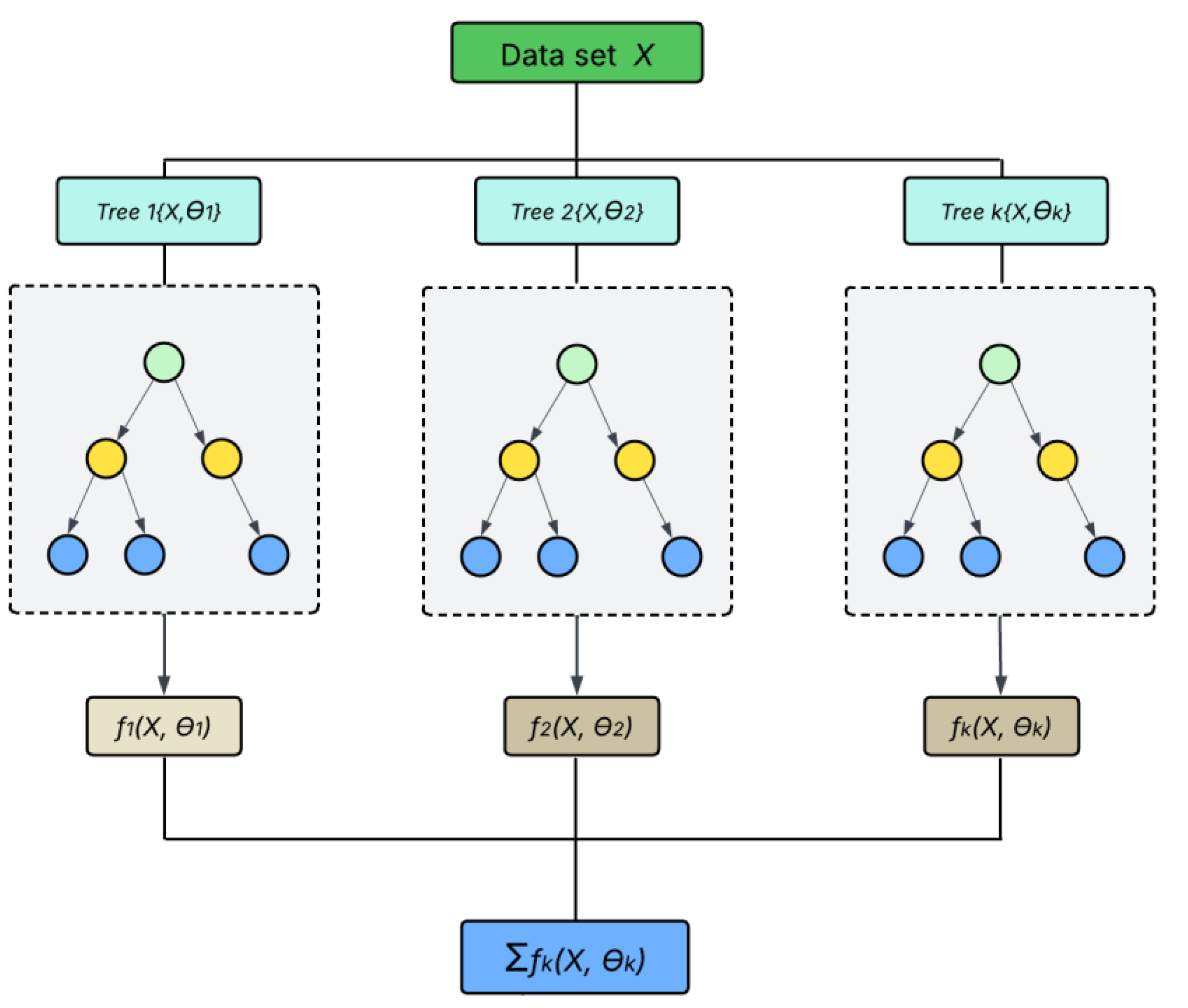
2.5. General XGBoost architecture
XGBoost is an ensemble learning method derived from regular gradient boosting method. It uses sequential decision trees as base learners with each tree responsible for correcting errors made by the previous tree in the process called boosting, thereby a good choice for time series data. Figure 4 presents the general XGBoost workflow.
Figure 3.
General XGBoost architecture [29].
Figure 3.
General XGBoost architecture [29].
2.6. Proposed XGBoost architecture
The proposed XGBoost model architecture is configured with key hyperparameters optimized for stability and performance, as shown in Table 3. It uses 500 boosting rounds (n_estimators = 500) to iteratively improve model accuracy, with a learning rate of 0.05 to control the step size and reduce the risk of overfitting. The maximum tree depth is set to 5 to balance model complexity and generalization. A fixed random seed (random_state = 42) ensures reproducibility of results across runs.
2.7. Experiment setup
This study experiments evaluated standalone ML, DL and a hybrid ML-DL models in predicting soil moisture trends over 24-hour, 72-hour, and 168-hour prediction. Firstly, the ML models tested included; XGBoost, RF, GB, SVR, LightGBM, LR, ElasticNet, CatBoost, DT, MLP, AdaBoost, and KNN. Secondly, five DL architectures were tested including; GRU, CNN, RNN, Bi-LSTM, and LSTM. The LSTM model architecture comprised three stacked LSTM layers followed by a dropout and a dense layer, allowing it to effectively model long-term temporal dependencies.
The GRU model followed this structure but used GRU units, offering comparable performance with reduced computational overhead. The CNN model consisted of a sequence of 1D convolutional (Conv1D) and max-pooling layers to extract localized temporal features, followed by a flattening operation and dense layer for prediction. The RNN model used three recurrent layers and a dense output layer, providing a baseline for evaluating short-term dependency modeling. The Bi-LSTM model integrated three bidirectional LSTM layers, enabling the network to process input sequences in both forward and backward directions and capture richer contextual information. These DL architectures are summarized in Table 4.
Lastly, beyond standalone models, we also developed hybrid architectures that combined LSTM-based temporal feature extraction with machine learning regressors for final prediction. These hybrid models included combinations of LSTM with other models like RF, LR, XGBoost, KNN, MLP, DT and CNN. While in other cases LSTM was used for feature extraction before passing them to a regressor for final prediction, in CNN + LSTM model, CNN layers performed initial feature extraction before passing the sequence to LSTM layers for further temporal modeling and prediction.
Finally, we proposed a hybrid model combining LSTM for feature extraction with XGBoost for the final prediction task. This approach capitalizes on the temporal learning capabilities of LSTM and the robust, non-linear decision-making strength of XGBoost. All models were evaluated across the same multi-step horizons (24, 72, and 168 hours) to ensure consistent comparison. Table 4 presents the DL models architectures used in the study along with their structural details.
2.8. Proposed method architecture
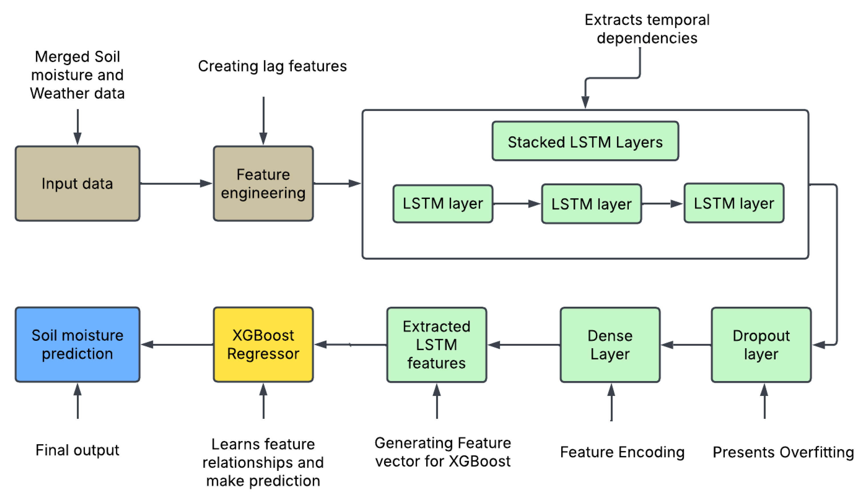
The proposed (LSTM + XGBoost) hybrid method consists of three sequentially stacked LSTM layers for temporal feature extraction, followed by dropout and dense layers for regularization and feature encoding, and finally an XGBoost regressor for final soil moisture prediction. The LSTM architecture begins with a 256-unit layer, followed by 128 and 64-unit LSTM layers, respectively. A dropout layer with a rate of 0.2 is applied after the final LSTM layer to mitigate the risk of overfitting by randomly deactivating neurons during training. The extracted temporal features are then passed through a dense layer with 64 units, serving as a compact encoded representation of the sequence. This feature vector is used as input to the XGBoost model, which performs the final multi-step soil moisture prediction. The LSTM model is trained using the Adam optimizer, ReLU activation function, and MSE loss over 100 epochs, using a (80%-20%) train -test split with 20% of the training data reserved for validation. The workflow for the proposed framework is shown in Figure 5.
Figure 5.
Proposed method architecture.
2.9. Model Performance Evaluation Metrics
We evaluated model performance using three common metrics: Coefficient of determination also known as the R-squared (R²), Mean Squared Error (MSE), and Mean Absolute Error (MAE). R² measures the proportion of variance in the dependent variable explained by the model, with values between 0 and 1 whereas the closer R² score is to 1, the better the model fits the data. MSE measures the average squared difference between predicted and actual values, where a lower MSE indicates better prediction accuracy while the MAE on the other hand, calculates the average magnitude of errors without considering their direction. It is less sensitive to outliers than MSE, making it suitable for cases where large errors should not overly impact model evaluation. The equations (7), (8) and (9) presents R2, MAE and MSE respectively;
where n is the number of samples, yi is the actual value for the i-th sample, ŷi is the predicted value for the i-th sample and y is the mean of the actual values.
2.10. Models training history
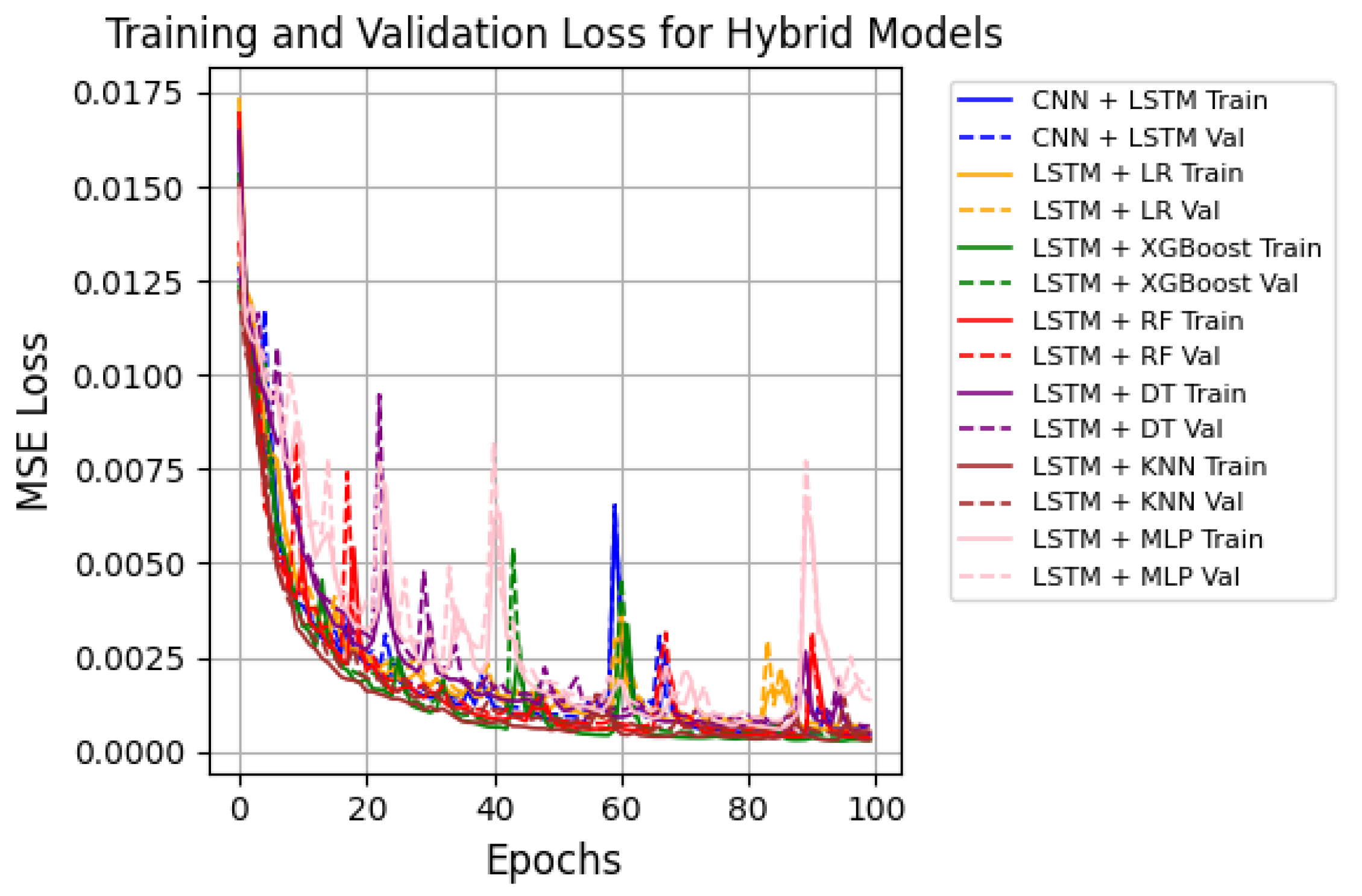
In summary, all DL and hybrid models were trained with a batch size of 32 and 100 epochs, demonstrating good generalization and convergence with a sharp decrease in MSE loss and increase in R2. Figure 6 and Figure 7 display the training and validation MSE loss curves for the proposed model and LSTM + RF, which recorded the second-best results, making it a useful benchmark for comparison. The training history of all hybrid models is shown in Figure 8. All models displayed effective learning, with error decreasing from approximately 0.0175 to near 0.0001. LSTM + XGBoost showed a smooth learning curve with minimal fluctuations, while LSTM + RF exhibited some loss variations but eventually converged as expected. A summary of the training history for all models is presented in Figure 8.
Figure 4.
MSE loss curve for LSTM + XGBoost.
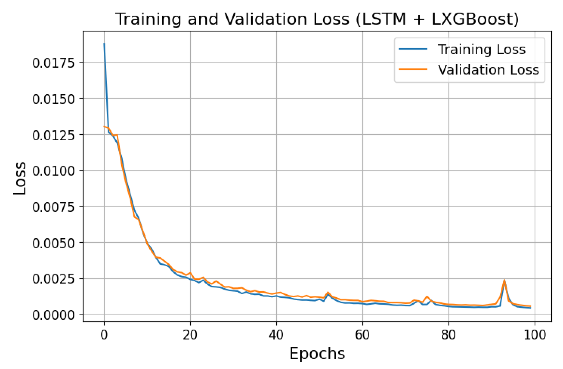
Figure 5.
MSE loss curve for LSTM + RF.
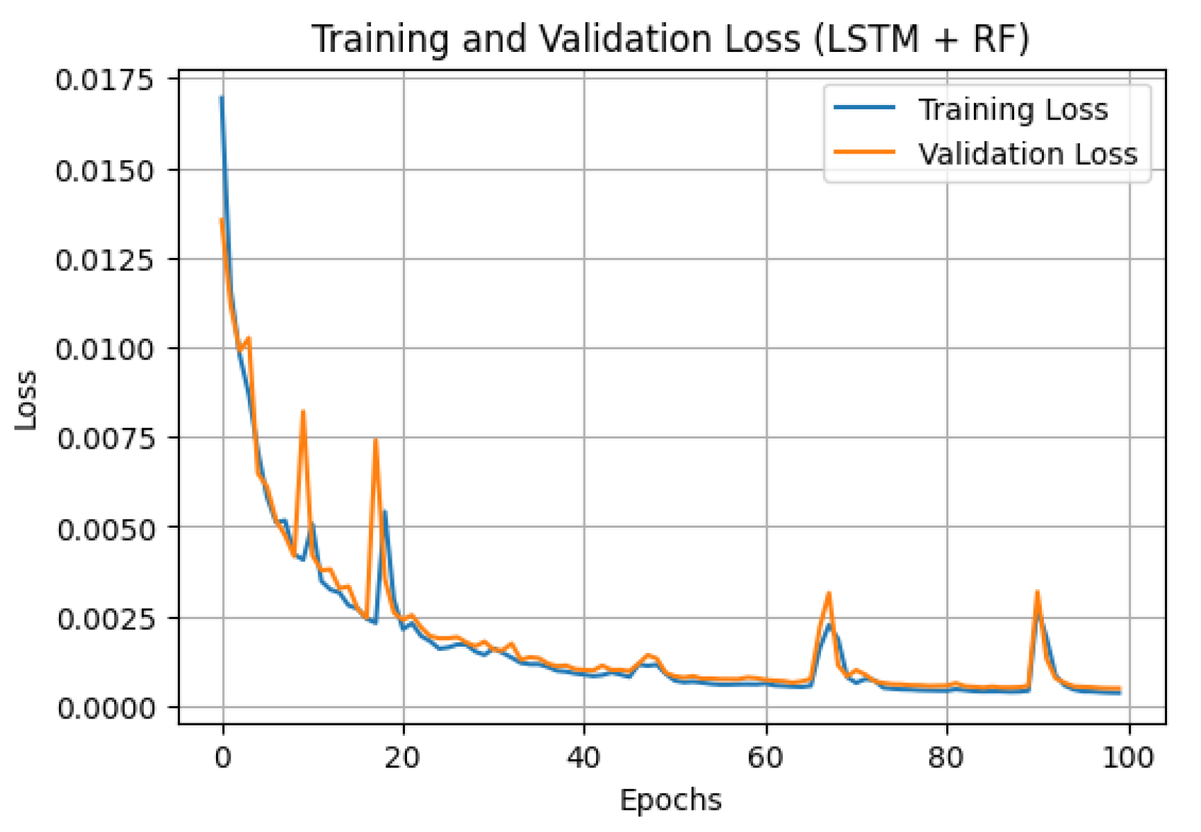
Figure 6.
MSE loss curves for all hybrid models.
3. Results
3.1. Standalone ML models result
Table 5 presents a summary result for multistep soil moisture prediction using standalone machine learning models for (24, 72 and 168) hour predictions. Results demonstrates that ET achieved the best performance recording (96.73%), (96.05%), and (95.60%) R2 values for 24 hours, 72 hours and 168 hours ahead respectively. It is followed closely by the RF which recorded (94.74%), (94.07%) and (91.73%) R2 scores for 24 hours, 72 hours and 168 hours ahead respectively while on the third place is the XGBoost model with (91.86%, 91.84% and 90.83%) R2 for 24 hours, 72 hours and 168 hours respectively. Additionally, these models showcase their superiority by recording lowest error scores led by ET that recorded average of (MAE = 0.4538 and MSE = 1.6417) while RF recorded an average of (MAE = 0.6793 and MSE = 2.1862). On the other hand, models like SVR recorded up to (MSE = 27.437 and MAE = 3.07), MLP (MSE = 26.781 and MAE = 3.5319), LR (MSE = 25.253 and MAE = 3.3593), and performed the worst recording. Overall results show that most standalone ML models generally do struggle to make multistep predictions unlike in single step (next hour predictions) due to dynamic and complex relationships between features that are exacerbated over time.
3.2. Standalone DL Models result
Table 6 presents the performance of DL models across 24-hour, 72-hour, and 168-hour prediction horizons. The results show that LSTM consistently achieved the best performance, with the highest R² scores across all prediction times, demonstrating its strong ability to capture temporal dependencies. The CNN model also performed competitively, closely matching LSTM in accuracy, particularly for short- and mid-range forecasts. While LSTM showed slightly higher error metrics, it maintained strong predictive capability. In contrast, the GRU and RNN models exhibited lower accuracy, especially over longer forecast horizons, highlighting their limitations in modeling complex temporal patterns in soil moisture dynamics.
3.3. Hybrid LSTM models result
Table 7 summarizes the performance of hybrid LSTM models across all prediction horizons. The LSTM + XGBoost combination consistently outperformed other hybrid approaches, achieving the highest R² scores (98.67%, 98.56%, and 98.54%) for 24 hours, 72 hours, and 168 hours, respectively. It was closely followed by the LSTM + RF and LSTM + KNN methods, both achieving over 98% R² values across all prediction horizons. The LSTM + MLP method performed the weakest but still achieved an average R² score above 92% for all three prediction horizons, outperforming most ML and some DL models, highlighting the strength of hybrid models. Additionally, hybrid models recorded the lowest error, with LSTM + XGBoost achieving MSE of 0.0002 and MAE of 0.0074 for the 168-hour prediction.
In general, the experiment results suggest that, hybrid LSTM models have the highest R² scores across all time steps compared to standalone ML and DL models. Specifically, the proposed model (LSTM + XGBoost) results demonstrate its effectiveness in capturing non-linear relationships using LSTM-extracted temporal features. Overall, the results highlight the advantage of integrating LSTM with robust ML regressors, particularly tree-based models like XGBoost, RF and KNN for improved multistep soil moisture prediction.
3.4. Model testing (Actual vs Prediction results) visualization
We evaluated model performance using a uniform sample size with normalized actual soil moisture values from the test set, focusing on the 168-hour prediction. Figure 9 shows the performance of the top-performing standalone ML (since there were too many ML models, we only selected the top performing models to maintain clarity and readability) including; ET, RF, and XGBoost chosen for their higher R² scores. Figure 10 and 11 represent DL and hybrid models respectively whereby in this case we presented all models since there were not as many ML models.
4. Discussion
This study evaluates a range of standalone ML, DL, and hybrid models for multistep soil moisture prediction. ML models, including ET, RF, and XGBoost, showed strong performance, with ET achieving the highest R² scores of 96.73%, 96.05%, and 95.60% for 24-hour, 72-hour, and 168-hour predictions, respectively, along with the lowest error (MAE = 0.4538, MSE = 1.6417). However, ML models generally exhibited higher error and lower R² as the prediction horizon extended. Models like SVR, MLP, and LR had even higher errors, especially at the 168-hour prediction (MSE up to 27 for SVR and 26 for MLP), underscoring the challenges of accurate multistep predictions using standalone ML models.
In contrast, DL models, particularly LSTM, outperformed others, with the highest R² values of 0.9762, 0.9752, and 0.9727 for 24-hour, 72-hour, and 168-hour predictions. CNN and Bi-LSTM also performed well but with slightly higher error metrics. GRU and RNN showed comparatively lower performance, especially for longer predictions. These results highlight the superior ability of LSTM, in particular, to capture temporal dependencies in soil moisture data for multistep predictions.
Finally, the hybrid LSTM models demonstrated the advantages of combining LSTM with traditional ML regressors. LSTM + XGBoost achieved the highest performance, with R² scores of 98.67%, 98.54%, and 98.56% for 24-hour, 72-hour, and 168-hour predictions, respectively, outperforming other hybrid combinations. Models like LSTM + RF and LSTM + KNN also performed well, with R² scores consistently above 98% across all time horizons. These hybrid models demonstrated significantly lower MSE and MAE compared to standalone ML and DL models. LSTM + XGBoost achieved 0.0002 MSE and 0.0074 MAE for 168-hour predictions, showcasing its robustness in capturing complex non-linear relationships and temporal dependencies. However, in the event of sudden heavy rains, soil moisture levels can experience abrupt spikes that could be challenging to capture with existing models; therefore, future works should focus on enhancing model responsiveness to extreme precipitation events using weather prediction models.
Overall, the results emphasize the effectiveness of hybrid models, particularly LSTM + XGBoost, in improving the accuracy of soil moisture predictions over extended periods. These models outperform standalone ML and DL models and provide a more reliable solution for optimizing irrigation scheduling and water-use efficiency in smart agriculture systems.
5. Conclusion
This study demonstrates the effectiveness of hybrid models, proposing an LSTM + XGBoost method, in predicting soil moisture content across multiple time horizons, showing significant improvements over both traditional ML and DL models. Standalone ML models are effective for short-term predictions (up to 24 hours) but struggle with longer multistep forecasts due to their inability to learn complex and dynamic relationships between features. In contrast, DL models capture temporal dependencies more effectively, yet hybrid models outperform both ML and DL models. The proposed LSTM + XGBoost hybrid method achieved superior performance, with R² scores of 98.67%, 98.54%, and 98.56% for 24, 72, and 168 hours, respectively, outperforming both standalone models.
Generally, hybrid models also recorded the lowest MSE and MAE across all prediction time horizons, highlighting their robustness in handling non-linear relationships and temporal dependencies between features. The results underscore the potential of hybrid approaches specifically the proposed model for soil moisture prediction, offering enhanced accuracy for optimizing irrigation scheduling and improving water-use efficiency in precision agriculture.
Author Contributions
D.K. conceptualized the study, developed the methodology, implemented the models, collected and curated the data, performed the formal analysis, and drafted the original manuscript. G.R, W.P., E.P., and A.M. provided technical guidance on methodology development and domain-specific input throughout the research process. D.Ki. and A.P. contributed to reviewing and improving the manuscript through proofreading and editorial suggestions. G.R. supervised the project, supported its administration, and secured the research funding. All authors have read and agreed to the published version of the manuscript.
Funding
This research was funded by the U.S. Department of Agriculture, National Institute of Food and Agriculture (USDA-NIFA), grant number 2023-68016-39403.
Data Availability Statement
All data generated, analyzed and experimented to support reported results of this study will be publicly available through an online repository at the project’s website through this link https://4dfarm.org/data/.
Acknowledgments
The authors sincerely appreciate the support of the U.S. Department of Agriculture, National Institute of Food and Agriculture (USDA-NIFA), for funding this research.
Conflicts of Interest
The authors declare no conflicts of interest.
Abbreviations
The following abbreviations are used in this manuscript:
| XGBoost | Extreme Gradient Boosting |
| RF | Random Forest |
| GB | Gradient Boosting |
| SVR | Support Vector Regressor |
| LightGBM | Light Gradient Boosting Method |
| LR | Linear Regression |
| DT | Decision Tree |
| MLP | Multi-Layer Perceptron |
| KNN | K-Nearest Neighbors |
| Bi-LSTM | Bi-directional Long Short Term Memory |
| LSTM | Long Short Term Memory |
| GRU | Gate Rated Unit |
| RNN | Recurrent Neural Network |
| DL | Deep Learning |
| ML | Machine Learning |
| ARIMA | AutoRegressive Intergrated Moving Averages |
| ET | Extra Trees |
| RR | Ridge Regression |
| CNN | Convolutional Neural Networks |
| ABAC | Abraham Baldwins Agricultural College |
References
- J. P. Walker, G. R. Willgoose, and J. D. Kalma, “In situ measurement of soil moisture: A comparison of techniques,” J Hydrol (Amst), vol. 293, no. 1–4, pp. 85–99, Jun. 2004, . [CrossRef]
- M. Schönauer et al., “Spatio-temporal prediction of soil moisture and soil strength by depth-to-water maps,” International Journal of Applied Earth Observation and Geoinformation, vol. 105, Dec. 2021, . [CrossRef]
- Y. Wang, L. Shi, Y. Hu, X. Hu, W. Song, and L. Wang, “A comprehensive study of deep learning for soil moisture prediction,” Hydrol Earth Syst Sci, vol. 28, no. 4, pp. 917–943, Feb. 2024, . [CrossRef]
- A. Rani, N. Kumar, J. Kumar, J. Kumar, and N. K. Sinha, “Chapter 6 - Machine learning for soil moisture assessment,” in Deep Learning for Sustainable Agriculture, R. C. Poonia, V. Singh, and S. R. Nayak, Eds., Academic Press, 2022, pp. 143–168. [CrossRef]
- K. Dolaptsis et al., “A Hybrid LSTM Approach for Irrigation Scheduling in Maize Crop,” Agriculture (Switzerland), vol. 14, no. 2, Feb. 2024, . [CrossRef]
- F. Granata, F. Di Nunno, M. Najafzadeh, and I. Demir, “A Stacked Machine Learning Algorithm for Multi-Step Ahead Prediction of Soil Moisture,” Hydrology, vol. 10, no. 1, Jan. 2023, . [CrossRef]
- Q. Li, Y. Zhu, W. Shangguan, X. Wang, L. Li, and F. Yu, “An attention-aware LSTM model for soil moisture and soil temperature prediction,” Geoderma, vol. 409, Mar. 2022, . [CrossRef]
- F. T. Teshome, H. K. Bayabil, B. Schaffer, Y. Ampatzidis, and G. Hoogenboom, “Improving soil moisture prediction with deep learning and machine learning models,” Comput Electron Agric, vol. 226, p. 109414, 2024, . [CrossRef]
- R. Togneri et al., “Soil moisture forecast for smart irrigation: The primetime for machine learning,” Expert Syst Appl, vol. 207, Nov. 2022, . [CrossRef]
- S. Ahmad, A. Kalra, and H. Stephen, “Estimating soil moisture using remote sensing data: A machine learning approach,” Adv Water Resour, vol. 33, no. 1, pp. 69–80, Jan. 2010, . [CrossRef]
- Y. Cai, W. Zheng, X. Zhang, L. Zhangzhong, and X. Xue, “Research on soil moisture prediction model based on deep learning,” PLoS One, vol. 14, no. 4, Apr. 2019, . [CrossRef]
- U. Acharya, A. L. M. Daigh, and P. G. Oduor, “Machine learning for predicting field soil moisture using soil, crop, and nearby weather station data in the red river valley of the north,” Soil Syst, vol. 5, no. 4, Dec. 2021, . [CrossRef]
- Z. Wu et al., “Estimating soil moisture content in citrus orchards using multi-temporal sentinel-1A data-based LSTM and PSO-LSTM models,” J Hydrol (Amst), vol. 637, Jun. 2024, . [CrossRef]
- R. Prasad, R. C. Deo, Y. Li, and T. Maraseni, “Soil moisture forecasting by a hybrid machine learning technique: ELM integrated with ensemble empirical mode decomposition,” Geoderma, vol. 330, pp. 136–161, Nov. 2018, . [CrossRef]
- P. Datta and S. A. Faroughi, “A multihead LSTM technique for prognostic prediction of soil moisture,” Geoderma, vol. 433, May 2023, . [CrossRef]
- K. KHOSRAVI et al., “Multi-step ahead soil temperature forecasting at different depths based on meteorological data: Integrating resampling algorithms and machine learning models,” Pedosphere, vol. 33, no. 3, pp. 479–495, Jun. 2023, . [CrossRef]
- Q. Li, C. Zhang, W. Shangguan, L. Li, and Y. Dai, “A novel local-global dependency deep learning model for soil mapping,” Geoderma, vol. 438, Oct. 2023, . [CrossRef]
- S. Kouadri, C. B. Pande, B. Panneerselvam, K. N. Moharir, and A. Elbeltagi, “Prediction of irrigation groundwater quality parameters using ANN, LSTM, and MLR models,” Environmental Science and Pollution Research, vol. 29, no. 14, pp. 21067–21091, Mar. 2022, . [CrossRef]
- D. F. Kandamali, X. Cao, M. Tian, Z. Jin, H. Dong, and K. Yu, “ Machine learning methods for identification and classification of events in ϕ -OTDR systems: a review ,” Appl Opt, vol. 61, no. 11, p. 2975, 2022, . [CrossRef]
- A. F. Jimenez, B. V. Ortiz, L. Bondesan, G. Morata, and D. Damianidis, “Long Short-Term Memory Neural Network for irrigation management: a case study from Southern Alabama, USA,” Precis Agric, vol. 22, no. 2, pp. 475–492, Apr. 2021, . [CrossRef]
- N. Filipović, S. Brdar, G. Mimić, O. Marko, and V. Crnojević, “Regional soil moisture prediction system based on Long Short-Term Memory network,” Biosyst Eng, vol. 213, pp. 30–38, Jan. 2022, . [CrossRef]
- P. Suebsombut, A. Sekhari, P. Sureephong, A. Belhi, and A. Bouras, “Field data forecasting using lstm and bi-lstm approaches,” Applied Sciences (Switzerland), vol. 11, no. 24, Dec. 2021, . [CrossRef]
- P. Gao et al., “Improved soil moisture and electrical conductivity prediction of citrus orchards based on IoT using deep bidirectional lstm,” Agriculture (Switzerland), vol. 11, no. 7, Jul. 2021, . [CrossRef]
- F. Huang et al., “Interpreting Conv-LSTM for Spatio-Temporal Soil Moisture Prediction in China,” Agriculture (Switzerland), vol. 13, no. 5, May 2023, . [CrossRef]
- Q. Li, Z. Li, W. Shangguan, X. Wang, L. Li, and F. Yu, “Improving soil moisture prediction using a novel encoder-decoder model with residual learning,” Comput Electron Agric, vol. 195, Apr. 2022, . [CrossRef]
- S. Chatterjee, N. Dey, and S. Sen, “Soil moisture quantity prediction using optimized neural supported model for sustainable agricultural applications,” Sustainable Computing: Informatics and Systems, vol. 28, Dec. 2020, . [CrossRef]
- S. Heddam, “3 - New formulation for predicting soil moisture content using only soil temperature as predictor: multivariate adaptive regression splines versus random forest, multilayer perceptron neural network, M5Tree, and multiple linear regression,” in Water Engineering Modeling and Mathematic Tools, P. Samui, H. Bonakdari, and R. Deo, Eds., Elsevier, 2021, pp. 45–62. [CrossRef]
- T. O’shea, V. Tech, T. J. O’shea, S. Hitefield, and J. Corgan, “End-to-End Radio Traffic Sequence Recognition with Deep Recurrent Neural Networks,” 2016, . [CrossRef]
- R. Guo, Z. Zhao, T. Wang, G. Liu, J. Zhao, and D. Gao, “Degradation state recognition of piston pump based on ICEEMDAN and XGBoost,” Applied Sciences (Switzerland), vol. 10, no. 18, Sep. 2020, . [CrossRef]
Figure 9.
Actual vs predicted soil moisture values for 168-hours using standalone ML models.
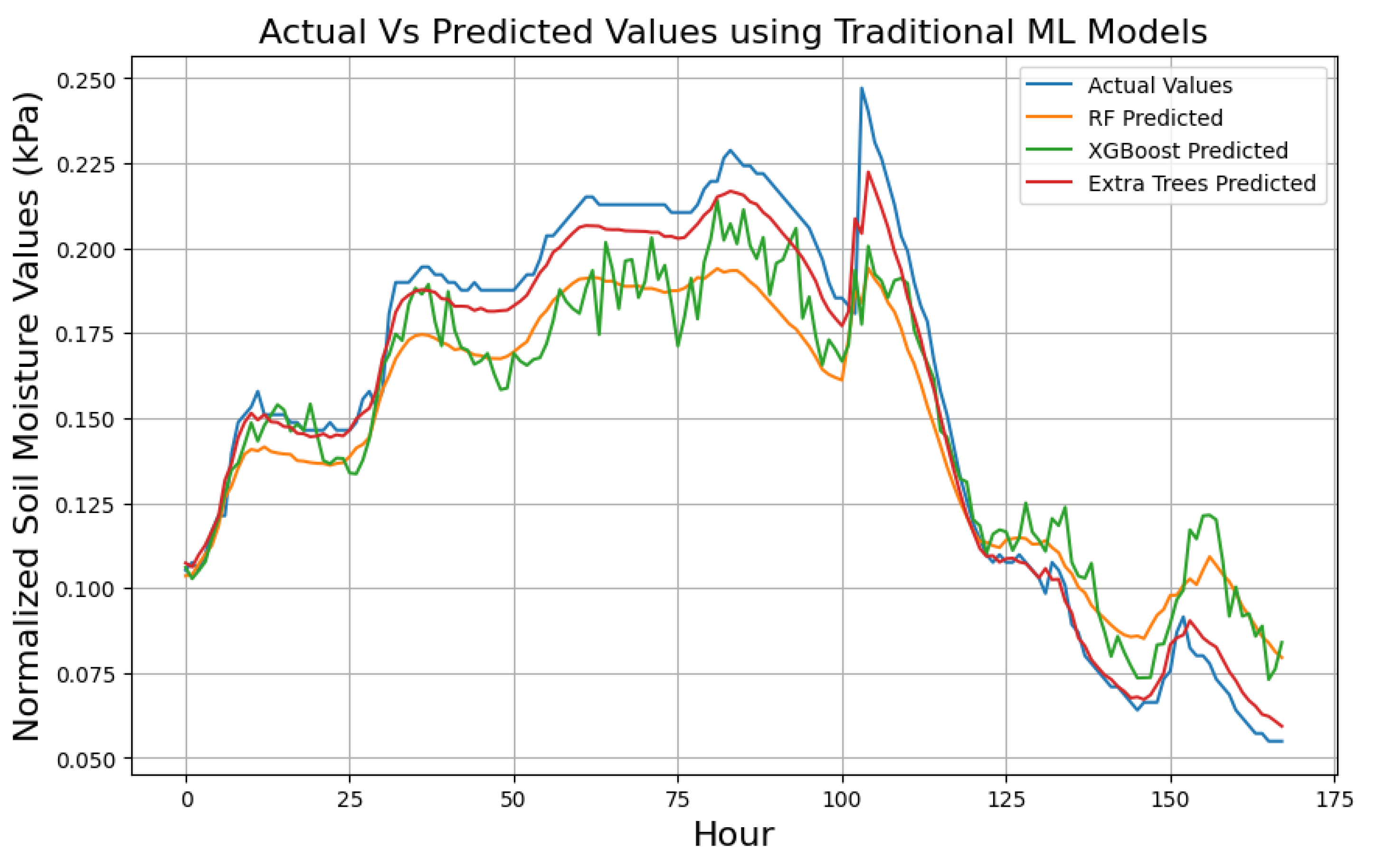
Figure 10.
Actual vs predicted soil moisture values for 168-hours using standalone DL models.
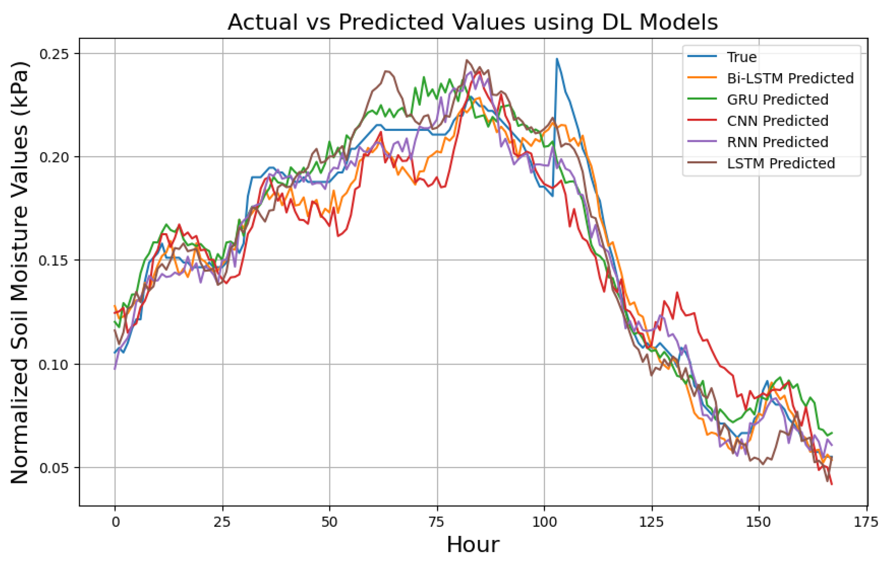
Figure 11.
Actual vs predicted soil moisture values for 168-hours using hybrid models.
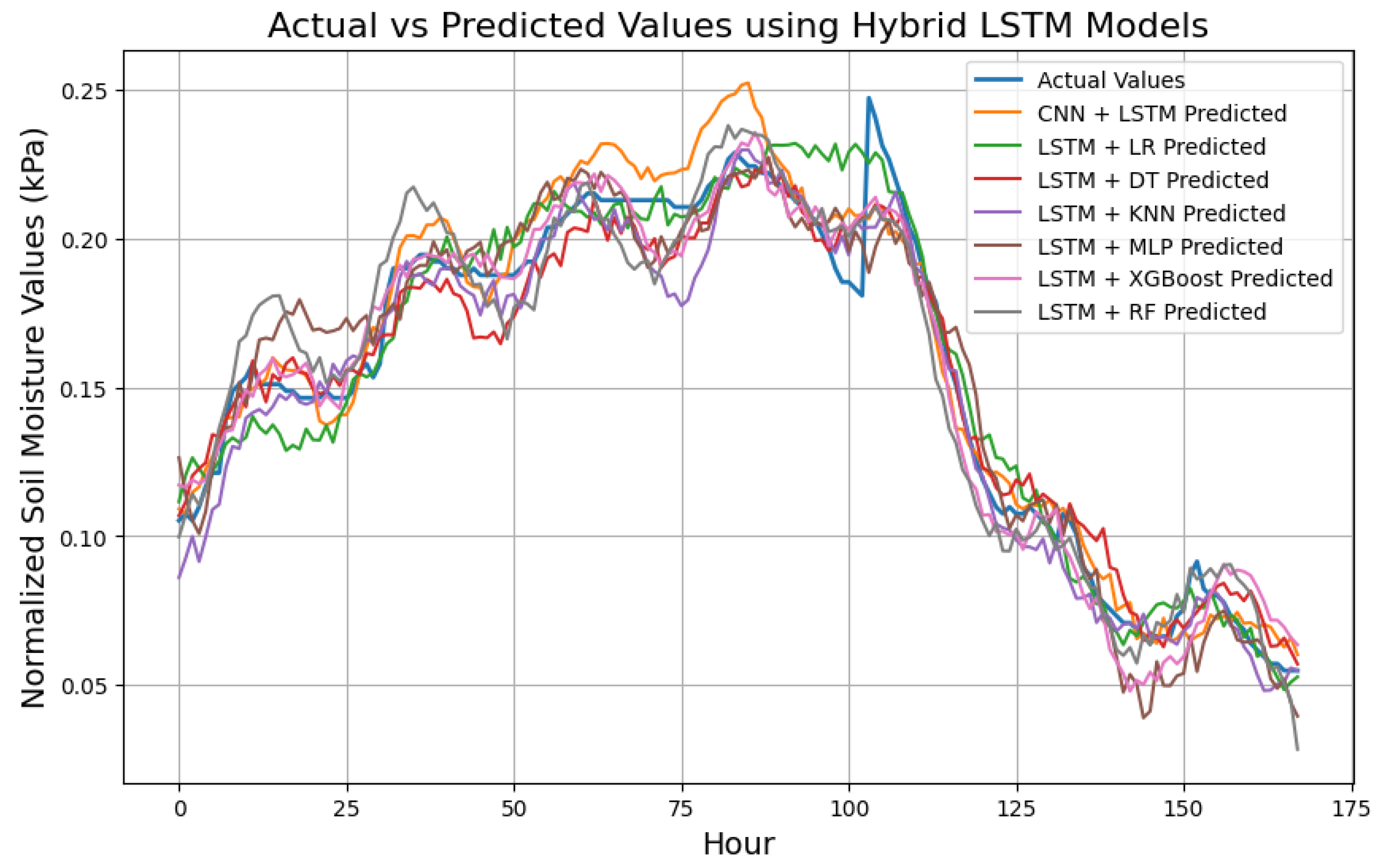

Table 1.
Watermark soil moistures and weather station distribution in the 4D D.A.T.A farm.
| Field Name | Device Name | Latitude | Longitude |
| Front Field | 4D01 | 31.48449 | -83.5452 |
| Front Field | 4D02 | 31.4845 | -83.544 |
| North Pivot | 4D03 | 31.4837728 | -83.5477376 |
| North Pivot | 4D04 | 31.4841216 | -83.5486016 |
| North Pivot | 4D05 | 31.4839808 | -83.5469888 |
| North Pivot | 4D06 | 31.4844096 | -83.5479488 |
| South Pivot | 4D07 | 31.4826464 | -83.5490432 |
| South Pivot | 4D08 | 31.4819584 | -83.5483456 |
| South Pivot | 4D09 | 31.4828736 | -83.54864 |
| South Pivot | 4D10 | 31.4822336 | -83.5472512 |
| West Field | 4D11 | 31.4814976 | -83.5514752 |
| West Field | 4D12 | 31.4814336 | -83.5508224 |
| West Field | 4D13 | 31.4826112 | -83.5502144 |
| West Field | 4D14 | 31.4826048 | -83.5510784 |
| Farm Weather Station | 31.48509752 | -83.54801174 | |
Table 2.
The proposed LSTM architecture.
| Layer | Output Shape | Parameters |
| LSTM | (32, 24, 256) | 271360 |
| LSTM | (32, 24, 128) | 197120 |
| LSTM | (32, 64) | 49408 |
| Dropout | (32, 64) | 0 |
| Dense | (32, 256) | 16640 |
| Dense | (32, 168) | 43296 |
Table 3.
Proposed XGBoost architecture.
| Hyperparameter | Value | Description |
| n_estimators | 500 | Number of boosting rounds (trees). |
| learning_rate | 0.05 | Step size used in the update to prevent overfitting |
| max_depth | 5 | Maximum depth of trees |
| random_state | 42 | Random seed for reproducibility. |
Table 4.
DL models architecture.
| Model | Layers | Output |
| LSTM | LSTM → LSTM → LSTM → Dropout→ Dense → Output | 168 time-steps |
| GRU | GRU → GRU → GRU → Dense → Output | 168 time-steps |
| CNN | Conv1D → MaxPooling → Conv1D → MaxPooling → Conv1D → Flatten → Dense → Output | 168 time-steps |
| RNN | RNN → RNN → RNN → Dense → Output | 168 time-steps |
| Bi-LSTM | Bi-LSTM → Bi-LSTM → Bi-LSTM → Dense → Output | 168 time-steps |
Table 5.
Multistep soil prediction results using Standalone ML models.
| 24 Hours | 72 Hours | 168 Hours | |||||||
| Model | MSE | MAE | R2 | MSE | MAE | R2 | MSE | MAE | R2 |
| RF | 2.1862 | 0.6793 | 0.9474 | 2.3530 | 0.8439 | 0.9407 | 2.6979 | 0.8953 | 0.9173 |
| SVR | 26.389 | 3.0212 | 0.3469 | 26.629 | 3.0228 | 0.3295 | 27.437 | 3.0700 | 0.3119 |
| DT | 5.7204 | 0.8667 | 0.8624 | 6.8018 | 0.9684 | 0.8286 | 6.9688 | 0.9640 | 0.7864 |
| GB | 3.9939 | 1.0681 | 0.9044 | 6.2844 | 1.6528 | 0.8380 | 6.6368 | 1.7598 | 0.7829 |
| MLP | 22.674 | 3.2572 | 0.4545 | 26.483 | 3.5384 | 0.3327 | 26.781 | 3.5319 | 0.1792 |
| LR | 11.671 | 1.7389 | 0.7192 | 23.604 | 3.0455 | 0.4052 | 25.253 | 3.3593 | 0.2260 |
| AdaBoost | 11.301 | 2.8148 | 0.7290 | 17.925 | 3.6179 | 0.5358 | 15.839 | 3.3744 | 0.4949 |
| ET | 1.6417 | 0.4538 | 0.9673 | 1.2966 | 0.5183 | 0.9605 | 1.4349 | 0.5450 | 0.9560 |
| RR | 11.667 | 1.7385 | 0.7208 | 23.598 | 3.0451 | 0.3902 | 25.247 | 3.3589 | 0.1779 |
| XGBoost | 3.3839 | 0.7440 | 0.9186 | 3.2386 | 0.9679 | 0.9184 | 3.3175 | 1.0118 | 0.9083 |
| ElasticNet | 11.198 | 1.6929 | 0.7306 | 22.536 | 2.9726 | 0.4322 | 23.895 | 3.2742 | 0.2677 |
Table 6.
Result summary for DL models in multistep soil moisture prediction.
| 24 Hours | 72 Hours | 168 Hours | |||||||
| Model | MSE | MAE | R2 | MSE | MAE | R2 | MSE | MAE | R2 |
| LSTM | 0.0007 | 0.0156 | 0.9781 | 0.0007 | 0.0158 | 0.9771 | 0.0006 | 0.0146 | 0.9738 |
| Bi-LSTM | 0.0005 | 0.0128 | 0.9662 | 0.0005 | 0.0126 | 0.9652 | 0.0005 | 0.0122 | 0.9627 |
| CNN | 0.0005 | 0.0136 | 0.9748 | 0.0005 | 0.0135 | 0.9741 | 0.0005 | 0.0131 | 0.9710 |
| GRU | 0.0014 | 0.0234 | 0.9311 | 0.0015 | 0.0228 | 0.9294 | 0.0015 | 0.0240 | 0.9098 |
| RNN | 0.0020 | 0.0269 | 0.9063 | 0.0023 | 0.0299 | 0.8878 | 0.0023 | 0.0301 | 0.8660 |
Table 7.
Result summary for Hybrid LSTM models for multistep soil moisture prediction.
| 24 Hours | 72 Hours | 168 Hours | |||||||
| Model | MSE | MAE | R2 | MSE | MAE | R2 | MSE | MAE | R2 |
| LSTM + RF | 0.0003 | 0.0086 | 0.9834 | 0.0004 | 0.0093 | 0.9827 | 0.0003 | 0.0082 | 0.9822 |
| LSTM + LR | 0.0006 | 0.0148 | 0.9719 | 0.0006 | 0.0153 | 0.9693 | 0.0006 | 0.0152 | 0.9652 |
| LSTM + XGBoost | 0.0003 | 0.0078 | 0.9867 | 0.0003 | 0.0080 | 0.9856 | 0.0002 | 0.0074 | 0.9854 |
| LSTM + KNN | 0.0003 | 0.0072 | 0.9838 | 0.0004 | 0.0078 | 0.9824 | 0.0003 | 0.0068 | 0.9821 |
| LSTM + MLP | 0.0015 | 0.0234 | 0.9271 | 0.0017 | 0.0239 | 0.9219 | 0.0014 | 0.0230 | 0.9193 |
| LSTM + DT | 0.0009 | 0.0108 | 0.9590 | 0.0009 | 0.0114 | 0.9579 | 0.0007 | 0.0102 | 0.9567 |
| CNN + LSTM | 0.0007 | 0.0151 | 0.9685 | 0.0006 | 0.0147 | 0.9699 | 0.0006 | 0.0150 | 0.9659 |
Disclaimer/Publisher’s Note: The statements, opinions and data contained in all publications are solely those of the individual author(s) and contributor(s) and not of MDPI and/or the editor(s). MDPI and/or the editor(s) disclaim responsibility for any injury to people or property resulting from any ideas, methods, instructions or products referred to in the content. |
© 2025 by the authors. Licensee MDPI, Basel, Switzerland. This article is an open access article distributed under the terms and conditions of the Creative Commons Attribution (CC BY) license (http://creativecommons.org/licenses/by/4.0/).
Copyright: This open access article is published under a Creative Commons CC BY 4.0 license, which permit the free download, distribution, and reuse, provided that the author and preprint are cited in any reuse.


