The Spacetime Algebra and Basic General Relativity

1. Foreword

This pedagogical paper was inspired by [1,2,3], which all outline notationally different yet equivalent methods of formulating General Relativity (GR) in the Spacetime Algebra (STA). However, while indeed more pedagogical than most papers and books (and still being excellent reads), a beginner would still find them to be difficult to parse. So the goal of this paper is to bridge the gap and present GR using STA in a geometrically-intuitive style, aimed for students and professors. It is the hope of the author that this paper can be a mostly self-contained crash-course to both the STA and using it for GR.1 Before continuing, the author would like to reiterate that [1,2,3] are excellent resources and should be read after this if more depth is desired.

The scope and study of GR is quite far-reaching, and presenting it in its entirety would undermine the pedagogical nature of this writ. Therefore the derivation of the Einstein equation from a stationary action will be ignored in favor of simply introducing the equation after deriving the curvature tensors (multivectors). Likewise the discussion of the Christoffel symbols will be limited to the presentation in Equation (4.22) and Equation (4.23). For more information on both the stationary action derivation and Christoffel symbols within the Geometric Algebra formalism, [1] is recommended with fervor.

2. Conceptual Overview

Conceptually, GR is not so complicated. It states that mass curves spacetime, which in turn modifies the dynamics. Constructing GR in the STA will be very straightforward: First, one must posit that every coordinate x infinitesimally close to another coordinate $x^{\prime }$ is related via an infinitesimal Lorentz transformation. Second, one must create a derivative and gradient which transform covariantly as one moves throughout coordinate space (thereby keeping tally of curvature that might or might not be there). Using these covariant derivatives (which represent parallel-transporting a multivector field, and therefore represent the action of the spacetime curvature on said field), one then builds the appropriate curvature multivectors (tensors). This ends up being the Einstein vector (tensor) which expresses the "curvature flux" through the hyperplane geometrically represented by the vector. Finally, one obtains the Einstein equation by setting the Einstein vector equal to the stress-energy vector (tensor). The stress-energy vector expresses the "energy flux" through the hyperplane of the vector. Thus, the Einstein equation is a statement that the energy flux2 results in a curvature flux.

3. The Spacetime Algebra

Both an algebraic and geometric interpretation are now to be given. Such a step was seen as necessary for the reader to fully grasp the approach to General Relativity (GR) in the Spacetime Algebra (STA). Moreover, including such an introduction will allow this document to serve as a mostly standalone text for learning the STA. This crash-course was written with reference to [1,4,5,6], with notation particularly inspired by [6].

3.1. Algebraic Essentials

The Spacetime Algebra is a real geometric (Clifford) algebra generated by the orthonormal vector basis

$${\gamma }_0,{\gamma }_1,{\gamma }_2,{\gamma }_3$$

(3.1)

which satisfies the inner product

$${\gamma }_{\mu }·{\gamma }_{\nu }={\displaystyle \frac{1}{2}}({\gamma }_{\mu }{\gamma }_{\nu }+{\gamma }_{\nu }{\gamma }_{\mu })={\eta }_{\mu \nu },$$

(3.2)

where ${\eta }_{\mu \nu }$ is the (mostly-minus) Minkowski metric, and $\mu ,\nu =0,1,2,3$. This implies that ${\gamma }_0^2=+1$, while ${\gamma }_1^2={\gamma }_2^2={\gamma }_3^2=-1$. As there is one unipotent basis vector with three anti-unipotent basis vectors, this algebra is denoted ${\mathbb{G}}_{1,3}$. Moreover, in the context of Minkowski geometric algebras, ${\mathbb{G}}_{1,n}$, positive squaring objects are referred to as timelike, negative squaring objects are referred to as spacelike, and nilpotent objects are referred to as lightlike. The basis in Equation (3.1) is called the standard basis, as opposed to the reciprocal basis

$${\gamma }^0,{\gamma }^1,{\gamma }^2,{\gamma }^3$$

(3.3)

which satisfies the inner product

$${\gamma }^{\mu }·{\gamma }_{\nu }={\displaystyle \frac{1}{2}}({\gamma }^{\mu }{\gamma }_{\nu }+{\gamma }_{\nu }{\gamma }^{\mu })={\delta }_{\nu }^{\mu },$$

(3.4)

where ${\delta }_{\nu }^{\mu }$ is the Kronecker delta. This implies ${\gamma }^j=-{\gamma }_j$ for $j=1,2,3$. Any vector a can be written as a linear combination of the standard basis

$$a=a^{\mu }{\gamma }_{\mu }=(a^0{\gamma }_0+a^1{\gamma }_1+a^2{\gamma }_2+a^3{\gamma }_3)$$

(3.5)

or of the reciprocal basis

$$a=a_{\mu }{\gamma }^{\mu }=(a_0{\gamma }^0+a_1{\gamma }^1+a_2{\gamma }^2+a_3{\gamma }^3).$$

(3.6)

Both Equation (3.5) and Equation (3.6) are given for consistency and to make it easier to connect to traditional formalisms. However, in general it is possible to work coordinate-free. The (geometric) product of any two vectors a and b is

$$ab=a·b+a\wedge b.$$

(3.7)

It is the sum of their inner product

$$a·b={\displaystyle \frac{1}{2}}(ab+ba)$$

(3.8)

and their outer product

$$a\wedge b={\displaystyle \frac{1}{2}}(ab-ba).$$

(3.9)

In coordinate form their inner product is $a·b=a^{\mu }{b}_{\mu }=a_{\mu }{b}^{\mu }$, and their outer product is $a\wedge b=a^{\mu }{b}^{\nu }{\gamma }_{\mu }{\gamma }_{\nu }(1-{\delta }_{\mu \nu })$. The quantities ${\gamma }_{\mu }{\gamma }_{\nu }={\gamma }_{\mu }\wedge {\gamma }_{\nu }={\gamma }_{\mu \nu }$ are the orthonormal basis bivectors,

$${\gamma }_{10},{\gamma }_{20},{\gamma }_{30},{\gamma }_{12},{\gamma }_{23},{\gamma }_{31}$$

(3.10)

where the ${\gamma }_{j0}$ are timelike and the ${\gamma }_{jk}$ are spacelike.

Before introducing the geometric product between bivectors, or between vectors and bivectors, a few concepts must be discussed. Firstly, geometric algebras are ${\mathbb{Z}}_2$-graded. Scalars are grade-0, vectors are grade-1, and bivectors are grade-2. For a d-dimensional algebra there are $d+1$ distinct grades, from grade-0 to grade-d, and in general a grade-k object is called a k-vector. Thus for the Spacetime Algebra, there are 5 grades, from grade-0 to grade-4. Scalars are grade-0, vectors are grade-1, and bivectors are grade-2. The orthonormal basis for trivectors, the grade-3 objects, is

$${\gamma }_{123},{\gamma }_{012},{\gamma }_{023},{\gamma }_{031}$$

(3.11)

and the basis for quadravectors, the grade-4 objects, is

$${\gamma }_{0123}.$$

(3.12)

Because there is only one basis element for grade-4, it is called the pseudoscalar3 and is relabeled as $I={\gamma }_{0123}$. The Spacetime Algebra can be written as the direct sum of its graded subspaces,

$${\mathbb{G}}_{1,3}=\underset{j=0}{\overset{4}{⨁}}{\mathbb{G}}_{1,3}^j={\mathbb{G}}_{1,3}^{0\oplus \dots \oplus 4}.$$

(3.13)

A general element of the Spacetime Algebra M is called a multivector, and is a linear combination of all bases, including 1, and the bases in Equation (3.1), Equation (3.10), Equation (3.11), and Equation (3.12). If $\mathrm{J}$ is the multivector index for this complete algebraic basis$\{1,{\gamma }_0,\dots ,{\gamma }_3,{\gamma }_{12},\dots ,{\gamma }_{30},{\gamma }_{123},\dots ,{\gamma }_{031},I\}$, then

$$M=M^{\mathrm{J}}{\gamma }_{\mathrm{J}}.$$

(3.14)

Alternatively, the grade projection can be defined as

$${〈M〉}_j\in {\mathbb{G}}_{1,3}^j,$$

(3.15)

satisfying

$${〈M〉}_{j\oplus k}={〈M〉}_j+{〈M〉}_k.$$

(3.16)

It is often convenient to express multivectors as the sum of their graded subcomponents, as will be seen in the upcoming discussion of conjugation. Another useful concept is that of blades. A j-blade is a grade-j object that can be expressed as the outer product of j vectors. For example, ${\gamma }_{12}$ is a 2-blade but ${\gamma }_{12}+{\gamma }_{30}$ is not. Combining the grade projector with the idea of blades enables a convenient definition of the geometric product between an arbitrary j-blade A and k-blade B,

$$AB={〈AB〉}_{|j-k|}+{〈AB〉}_{|j-k|+2}+\dots +{〈AB〉}_{j+k}.$$

(3.17)

Then the inner product is always the grade-lowering product

$$A·B={〈AB〉}_{|j-k|},$$

(3.18)

and the outer product is always the grade-raising product

$$A\wedge B={〈AB〉}_{j+k}.$$

(3.19)

The vector-bivector, trivector-trivector, and vector-trivector products can be easily extrapolated from Equation (3.17), and are seen to only contain the sum of their respective inner and outer products. The bivector-bivector product, however, includes an extra grade-preserving4 commutator product. That is, for bivectors B and $B^{\prime }$,

$$B{B}^{\prime }=B·B^{\prime }+[B,B^{\prime }]+B\wedge B^{\prime },$$

(3.20)

where the middle term is the commutator product,

$$[B,B^{\prime }]={\displaystyle \frac{1}{2}}(B{B}^{\prime }-B^{\prime }B).$$

(3.21)

Many geometric algebra sources denote the commutator product with the times operator, but this paper reserves that notation for the cross product,

$$B\times B^{\prime }=-[B,B^{\prime }]I,$$

(3.22)

which is equivalent to the Gibbs-Heaviside vector cross product.

3.1.1. Conjugations

There are three "grade-selective" (involutory) conjugations inherent to every geometric algebra. For a general multivector M the first is grade involution,

$$\widehat{M}={〈M〉}_0-{〈M〉}_1+{〈M〉}_2-{〈M〉}_3+{〈M〉}_4,$$

(3.23)

the second is reversion,

$$\tilde{M}={〈M〉}_0+{〈M〉}_1-{〈M〉}_2-{〈M〉}_3+{〈M〉}_4,$$

(3.24)

and the third is Clifford conjugation,

$$\overline{M}={〈M〉}_0-{〈M〉}_1-{〈M〉}_2+{〈M〉}_3+{〈M〉}_4.$$

(3.25)

Grade involution is so-named due to the fact it negates odd grades and ignores even grades. Reversion is so-named due to the fact it reverses all product orders. If N is also an arbitrary multivector, then $\widetilde{MN}=\tilde{N}\tilde{M}$. Clifford conjugation is the composition of grade involution and reversion, $\overline{M}=\widehat{\tilde{M}}=\tilde{\widehat{M}}$.

There are two additional conjugations which, unlike the first three, depend upon the use of a unit timelike vector. For convenience, the vector is chosen as ${\gamma }_0$. The first conjugation is parity conjugation,

$$M^{-}={\gamma }_{0}M{\gamma }_0,$$

(3.26)

and the second is Hermitian conjugation,

$$M^{†}={\gamma }_0\tilde{M}{\gamma }_0.$$

(3.27)

Both parity and Hermitian conjugation are well-known conjugations in physics. Geometrically, parity corresponds to the negative of a reflection in the ${\gamma }_0$ hyperplane defined in Section 3, while Hermitian conjugation corresponds to reversion followed by parity.

3.1.2. The Lorentz Group, $\mathrm{Spin}(1,3)$

At the heart of relativistic physics lies the Lorentz group, $\mathrm{Spin}(1,3)\approx \mathrm{SL}(2,\mathbb{C})$. This spin group exists naturally within the Spacetime Algebra,

$$\mathrm{Spin}(1,3)=\{\Lambda \in {\mathbb{G}}_{1,3}^{+}|\Lambda \tilde{\Lambda }=\tilde{\Lambda }\Lambda =1\},$$

(3.28)

where ${\mathbb{G}}_{1,3}^{+}={\mathbb{G}}_{1,3}^{0\oplus 2\oplus 4}$ is the even subalgebra of the Spacetime Algebra and $\Lambda$ is called a Lorentz rotor. The existence of this group is thanks to the basis bivectors of Equation (3.10), which form the Lie algebra $\mathfrak{spin}(1,3)\approx \mathfrak{sl}(2,\mathbb{C})$. In general, a Lorentz rotor is of the form

$$\Lambda =RL=e^{-{\displaystyle \frac{1}{2}}{B}_{\mathrm{sp}}}{e}^{{\displaystyle \frac{1}{2}}{B}_{\mathrm{ti}}}=e^{{\displaystyle \frac{1}{2}}\Omega },$$

(3.29)

where $B_{\mathrm{ti}}$ is a timelike bivector, $B_{\mathrm{sp}}$ is a spacelike bivector, and $\Omega =-B_{\mathrm{sp}}+B_{\mathrm{ti}}$ is the total5spacetime rotation rate. This means that R is a (Euclidean) rotation and L is a (Lorentz) boost. Note that in general, $LR\ne RL$. An arbitrary multivector is then Lorentz-transformed via a sandwich product,

$$M\mapsto \Lambda M\tilde{\Lambda }.$$

(3.30)

3.1.3. Duality in ${\mathbb{G}}_{1,3}$

The pseudoscalar I functions as the generator of duality. This holds in arbitrary (non-degenerate) geometric algebras. For a multivector M in the Spacetime Algebra,

$$★:M\mapsto M{I}^{-1}=-MI$$

(3.31)

is the duality map. In the Spacetime Algebra, this maps scalars to pseudoscalars, vectors to trivectors, timelike bivectors to spacelike bivectors, trivectors to vectors, and pseudoscalars to scalars. As the pseudoscalar is the generator of this duality, then maps of either the form (for $\theta \in \mathbb{R}$)

$$M\mapsto e^{\theta I}M$$

(3.32)

or

$$M\mapsto e^{{\displaystyle \frac{1}{2}}\theta I}M{e}^{-{\displaystyle \frac{1}{2}}\theta I}$$

(3.33)

are called duality rotations. Notice that Equation (3.33) leaves even-graded multivectors invariant.

3.2. The Mirror-Based View

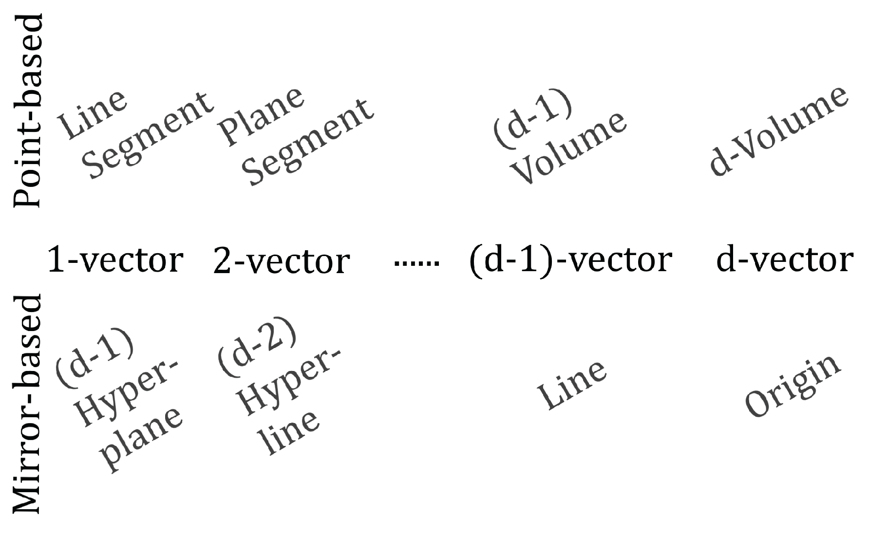
Geometric algebras are traditionally described in the point-based view which does not holistically incorporate geometric objects like space itself, hyperplanes, hyperlines, lines, or points as being represented by graded objects. The mirror-based view, which employs a top-down approach to geometry does exactly this. As shown in Figure 1. For a $(p+q)$-dimensional6 real geometric algebra, $d=p+q$ is the dimension of the (pseudo)Euclidean space. Vectors always represent $(d-1)$-dimensional hyperplanes, bivectors represent $(d-2)$-dimensional hyperlines. This pattern continues until $(d-1)$-vectors give 1-dimensional lines and d-vectors give 0-dimensional points.

If $A,B\in {\mathbb{G}}_{p,q}$ are respectively a j-blade and k-blade, then their outer product as specified by Equation (3.19) represents the subspace intersection of the two blades. Similarly, their outer product as specified by Equation (3.18) represents the subspace orthogonal to the higher graded blade which contains the subspace of the lower graded blade. If ★ represents the duality map like in Equation (3.31) then the regressive product is

$$A\vee B={★}^{-1}(★A\wedge ★B)$$

(3.34)

and represents the join of the two blades’ subspaces.

As all algebraic objects correspond to geometric objects within the mirror-based view, the geometric interpretation of real scalars is a natural question. The apparent answer to this question is that real scalars represent the space itself. Conceptually, this is a rather clever solution. Geometric objects in the space have orientations relative to the space, but the space cannot have an orientation with respect to itself that differs from plus-or-minus unity. Moreover, the scaling of any geometric object is equivalent to an outer product. That is, if $\alpha$ is a real scalar and M is some multivector (in any algebra), then

$$\alpha \wedge M=\alpha M.$$

(3.35)

This implies an interpretation of coefficients as intersections between geometric objects with scalar fields intrinsic to the space they inhabit. Furthermore, since the multivector is "preserved" on both sides of Equation (3.35), the intersection of a multivector with the space itself returns the multivector. That is, the operation $1\wedge M=M$ acts as the identity intersection.

4. General Relativity

As stated in the conceptual overview of Section 2, constructing General Relativity (GR) in the Spacetime Algebra (STA) will be very straightforward: Starting with infinitesimal Lorentz transformations and building up to the Einstein equation. If the reader has not yet read about the algebraic and geometric essentials presented in Section 3, it is recommended reading.

4.1. Tetrad Bases

When working with curved manifolds, there are objects called tangent spaces. If $\mathcal{M}$ is the manifold, then $T_x\mathcal{M}$ is the tangent space at coordinate x. Since the approach of this paper is to work with the (geometric) Spacetime Algebra (STA), the notation from [3] will be adopted: Promoting the tangent space to a tangent geometric algebra is labeled by $G{T}_x\mathcal{M}={\mathbb{G}}_{1,3}\left(x\right)$, and called the geometric tangent space (GTS).

Without reference to a specific GTS, the coordinate x is a vector in the STA,

$$x=x^{\mu }{\gamma }_{\mu }=x_{\mu }{\gamma }^{\mu }.$$

(4.1)

Recall, the standard basis $\left\{{\gamma }_{\mu }\right\}$ of the STA is given by Equation (3.1) and the reciprocal basis $\left\{{\gamma }^{\mu }\right\}$ of the STA in Equation (3.3). When moving to the GTS $G{T}_x\mathcal{M}$, one shifts from the standard basis to the coordinate basis$\left\{g_{\alpha }\right\}$ defined by

$$g_{\alpha }={\partial }_{\alpha }x,$$

(4.2)

and from the reciprocal basis to the reciprocal coordinate basis $\left\{g^{\mu }\right\}$ defined by

$$g^{\alpha }·g_{\beta }={\delta }_{\beta }^{\alpha }.$$

(4.3)

Here, ${\partial }_{\alpha }=g_{\alpha }·\partial$ is the spacetime derivative in the $g_{\alpha }$ direction. This derivative is dependent upon the definition of the spacetime gradient,

$$\partial ={\gamma }^{\mu }{\partial }_{\mu }={\gamma }^{\mu }{\displaystyle \frac{\partial }{\partial x^{\mu }}}.$$

(4.4)

It might appear recursive to define the coordinate basis $\left\{g_{\alpha }\right\}$ in terms of $g_{\alpha }·\partial$, and it is! But it is not a problem. In practice, ${\partial }_{\alpha }$ is defined first and then $\left\{g_{\alpha }\right\}$ follows. An example is with polar coordinates: First the indices are defined as $\alpha =t,r,\theta ,\varphi$ and correspond with the scalar values t (time), r (radius), $\theta$ (polar angle), and $\varphi$ (azimuthal angle). Then ${\partial }_{\alpha }$ is the derivative with respect to each scalar value. So if the coordinate vector is given in polar coordinates

$$x=t{\gamma }_0+rsin\theta (cos\varphi {\gamma }_1+sin\varphi {\gamma }_2)+rcos\theta {\gamma }_3,$$

then

$$\begin{array}{cc}\hfill g_t& ={\gamma }_0\hfill \\ \hfill g_r& =sin\theta (cos\varphi {\gamma }_1+sin\varphi {\gamma }_2)+cos\theta {\gamma }_3\hfill \\ \hfill g_{\theta }& =rcos\theta (cos\varphi {\gamma }_1+sin\varphi {\gamma }_2)-rsin\theta {\gamma }_3\hfill \\ \hfill g_{\varphi }& =rsin\theta (-sin\varphi {\gamma }_1+cos\varphi {\gamma }_2)\hfill \end{array}$$

(4.5)

is the coordinate basis. It is important to realize that the difference in notation will tell whether or not one is working with the coordinate basis or the standard basis: This paper’s convention uses ${\partial }_{\alpha }$ only for $g_{\alpha }·\partial$, and ${\partial }_{\mu }$ only for $\partial /\partial x^{\mu }$. A big selling point for Geometric Algebra is the fact that everything can be coordinate-free (as exemplified in $g^{\alpha }{\partial }_{\alpha }={\gamma }^{\mu }{\partial }_{\mu }$), but it is not always easiest to learn a subject coordinate-free. For a beginner, whatever coordinate system is being used could be quite ambiguous, thus the difference between the coordinate indices $\alpha$ and standard indices $\mu$ is useful.

The inner product of Equation (3.8) defines the (coordinate) metric tensor,

$$g_{\alpha \beta }=g_{\alpha }·g_{\beta }.$$

(4.6)

The metric tensor therefore has an elegant interpretation within the STA: The mutual overlap of the different coordinate basis vectors. Moreover, it is easy to see that the symmetric nature of the metric tensor comes from the fact that the inner product of two vectors is symmetric!

In general, $\left\{g_{\alpha }\right\}$ is non-orthonormal. But one can move into an orthonormal basis at coordinate x. This new basis is called the tetrad of x, $\left\{{\underline{\gamma }}_m\right\}$. The tetrad satisfies

$${\underline{\gamma }}_m·{\underline{\gamma }}_n={\eta }_{mn},$$

(4.7)

where ${\eta }_{mn}$ is the usual Minkowski metric, like in Equation (3.2). No matter the coordinate indices $\alpha ={\alpha }_0,{\alpha }_1,{\alpha }_2,{\alpha }_3$, the tetrad indices are $m=0,1,2,3$, as is the case with the standard basis indices $\mu =0,1,2,3$. The tetrad thereby functions as a basis for a local STA at coordinate x, ${\mathbb{G}}_{1,3}\left(x\right)$, which is just the GTS $G{T}_x\mathcal{M}$. In order to notationally distinguish the tetrad from the standard basis, the reader will notice an underbar is given and Latin indices replace Greek indices. But how does one move into a tetrad $\left\{{\underline{\gamma }}_m\right\}$ from a coordinate basis $\left\{g_{\alpha }\right\}$? Via the vierbein $\left\{e_{\alpha }^m\right\}$ and $\left\{{\underline{e}}_m^{\alpha }\right\}$:

$$g_{\alpha }=e_{\alpha }^m{\underline{\gamma }}_m\mathrm{and}{g}^{\alpha }={\underline{e}}_m^{\alpha }{\underline{\gamma }}^m.$$

(4.8)

The vierbein are like the positive square roots of the respective metric tensors $g_{\alpha \beta }$ and $g^{\alpha \beta }$. Notice that Equation (4.8) is equivalent to

$${\underline{e}}_m^{\alpha }{g}_{\alpha }={\underline{\gamma }}_m\mathrm{and}{e}_{\alpha }^m{g}^{\alpha }={\underline{\gamma }}^m.$$

(4.9)

As a last note, all bases and their reciprocals satisfy the following,

$$g^{\alpha }·g_{\beta }={\delta }_{\beta }^{\alpha }\mathrm{and}{\underline{\gamma }}^m·{\underline{\gamma }}_n={\delta }_n^m.$$

(4.10)

And

$$e_{\alpha }^m{\underline{e}}_n^{\alpha }={\delta }_n^m\mathrm{and}{e}_{\alpha }^m{\underline{e}}_m^{\beta }={\delta }_{\alpha }^{\beta }$$

(4.11)

hold for the vierbein.

To better understand these concepts, the metric tensor $g^{\alpha \beta }$, vierbein $\left\{e_{\alpha }^m\right\}$, and tetrad ${\underline{\gamma }}_m$ will now be calculated for Equation (4.5) (the coordinate basis in polar coordinates). Directly from the inner products $g^{\alpha }·g^{\beta }$,

$$g^{\alpha \beta }\leftrightarrow \left\{\begin{array}{cccc}1& 0& 0& 0\\ 0& -1& 0& 0\\ 0& 0& {\displaystyle \frac{1}{-r^2}}& 0\\ 0& 0& 0& {\displaystyle \frac{1}{-r^2{sin}^2\theta }}\end{array}\right\}.$$

(4.12)

The vierbein (positive square root) is trivial since the metric tensor is diagonal:

$$\left\{{\underline{e}}_m^{\alpha }\right\}\leftrightarrow \left\{\begin{array}{cccc}1& 0& 0& 0\\ 0& 1& 0& 0\\ 0& 0& {\displaystyle \frac{1}{r}}& 0\\ 0& 0& 0& {\displaystyle \frac{1}{rsin\theta }}\end{array}\right\}.$$

(4.13)

Then the tetrad must be

$$\begin{array}{cc}\hfill {\underline{\gamma }}_0& =g_t={\gamma }_0\hfill \\ \hfill {\underline{\gamma }}_1& =g_r=sin\theta (cos\varphi {\gamma }_1+sin\varphi {\gamma }_2)+cos\theta {\gamma }_3\hfill \\ \hfill {\underline{\gamma }}_2& ={\displaystyle \frac{1}{r}}{g}_{\theta }=cos\theta (cos\varphi {\gamma }_1+sin\varphi {\gamma }_2)-sin\theta {\gamma }_3\hfill \\ \hfill {\underline{\gamma }}_3& ={\displaystyle \frac{1}{rsin\theta }}{g}_{\varphi }=(-sin\varphi {\gamma }_1+cos\varphi {\gamma }_2).\hfill \end{array}$$

(4.14)

4.2. The Covariant Derivative

Because GR deals with a curved manifold (presumably Spacetime), there must be a derivative operator which accounts for said curvature! It would be of the form

$$D_{\alpha }={\partial }_{\alpha }+\Gamma .$$

(4.15)

where ${\Gamma }_{\alpha }=\Gamma \left(g_{\alpha }\right)$ is some as-of-yet undefined connection (the curvature tally). But heuristically determining the connection is easy! This is due to GR’s curvature being bound by the following restriction: A coordinate x infinitesimally close to coordinate $x^{\prime }$ is related by an infinitesimal Lorentz transformation. That is, if ${\Lambda }_{ϵ}$ is an infinitesimal Lorentz rotor, and the coordinates x and $x^{\prime }$ are respectively given the tetrads $\left\{{\underline{\gamma }}_m\right\}$ and $\left\{{\underline{\gamma }}_m^{\prime }\right\}$, then

$${\underline{\gamma }}_m^{\prime }={\Lambda }_{ϵ}{\underline{\gamma }}_m{\tilde{\Lambda }}_{ϵ}.$$

(4.16)

Yet this form isn’t much use as it stands. The goal is to heuristically determine the connection $\Gamma$ by first observing the explicit form of an infinitesimal rotation (which bounds the curvature by the aforewritten restriction) and claiming that it is the connection! The explicit form of ${\Lambda }_{ϵ}$ can be determined by inserting an infinitesimal scalar $ϵ$ (such that ${ϵ}^n\approx 0$ for $n>1$) into Equation (3.29) and applying its Taylor expansion:

$${\Lambda }_{ϵ}=e^{{\displaystyle \frac{1}{2}}ϵ\Omega }=1+{\displaystyle \frac{1}{2}}ϵ\Omega .$$

(4.17)

Immediately plugging this into Equation (4.16),

$$\begin{array}{cc}\hfill (1+{\displaystyle \frac{1}{2}}ϵ\Omega ){\underline{\gamma }}_m(1-{\displaystyle \frac{1}{2}}ϵ\Omega )& \\ \hfill & ={\underline{\gamma }}_m+{\displaystyle \frac{1}{2}}ϵ\Omega {\underline{\gamma }}_m-{\displaystyle \frac{1}{2}}ϵ{\underline{\gamma }}_m\Omega -{\displaystyle \frac{1}{4}}{ϵ}^2\Omega {\underline{\gamma }}_m\Omega \hfill \\ \hfill & ={\underline{\gamma }}_m+ϵ[\Omega ,{\underline{\gamma }}_m],\hfill \end{array}$$

(4.18)

where the last step invoked the definition of the commutator product, Equation (3.21). Now the heuristic identification of the connection is

$${\Gamma }_{\alpha }=[{\Omega }_{\alpha },·],$$

(4.19)

where ${\Omega }_{\alpha }=\Omega \left(g_{\alpha }\right)$ is the connection bivector and $(·)$ represents the argument upon which the commutator acts. Therefore the covariant derivative is defined as

$$D_{\alpha }={\partial }_{\alpha }+[{\Omega }_{\alpha },·],$$

(4.20)

and then

$$D=g^{\alpha }{D}_{\alpha }$$

(4.21)

is the covariant gradient. The connection has a nice interpretation as the generator of the Lorentz transformation between two coordinates, and geometrically represents the act of rotating about the hyperline described by the spacetime rotation rate ${\Omega }_{\alpha }$.

4.2.1. The Connection Bivector

An expression for directly calculating the connection bivector ${\Omega }_{\alpha }$ is natural in the STA. However, discussion about the Christoffel symbols in the STA is warranted. Recall that the metric tensor $g_{\alpha \beta }$ is the inner product of $g_{\alpha }$ and $g_{\beta }$, and thereby measures their mutual overlap. The Christoffel symbols of GR are defined as

$${\Gamma }_{\alpha \beta }^{\delta }={\displaystyle \frac{1}{2}}{g}^{\delta \epsilon }\left({\partial }_{\alpha }{g}_{\beta \epsilon }+{\partial }_{\beta }{g}_{\alpha \epsilon }-{\partial }_{\epsilon }{g}_{\beta \alpha }\right).$$

(4.22)

In the parentheses, the first term is the rate of change of the overlap $g_{\beta \epsilon }$ in the $g_{\alpha }$ direction, the second term is the rate of change of the overlap $g_{\alpha \epsilon }$ in the $g_{\beta }$ direction, and the third term is the (negative) rate of change of the overlap $g_{\beta \alpha }$ in the $g_{\epsilon }$ direction. These rates are then summed over the (reciprocal) overlap $g^{\delta \epsilon }$. Therefore the Christoffel symbols are a measure of how changes in overlap within different directions affect the overlap in another direction. Christoffel symbols play an important role through the Christoffel identity,

$$D_{\beta }{g}_{\alpha }={\Gamma }_{\alpha \beta }^{\delta }{g}_{\delta },$$

(4.23)

and greatly simplify the calculation of the connection bivector ${\Omega }_{\alpha }$. The Christoffel identity is quite elegant, saying that the covariant change of the coordinate basis $\left\{g_{\alpha }\right\}$ is simply the measure of how changes in overlap within different directions affect the overlap in another direction.

Calculating the connection bivector is straightforward: Consider the covariant derivative of the tetrad $\left\{{\underline{\gamma }}_m\right\}$, then isolate ${\Omega }_{\alpha }$. First, the covariant derivative of the tetrad is taken directly, giving

$$\begin{array}{cc}\hfill D_{\beta }{\underline{\gamma }}_m& ={\partial }_{\beta }{\underline{\gamma }}_m+[{\Omega }_{\beta },{\underline{\gamma }}_m]\hfill \\ \hfill & =[{\Omega }_{\beta },{\underline{\gamma }}_m]\hfill \end{array}$$

(4.24)

since ${\partial }_{\beta }{\underline{\gamma }}_m=0$. Second, the covariant derivative of the tetrad expressed as the vierbein-coordinate product in Equation (4.9) is taken, giving

$$\begin{array}{cc}\hfill D_{\beta }{\underline{\gamma }}_m& =D_{\beta }\left({\underline{e}}_m^{\alpha }{g}_{\alpha }\right)\hfill \\ \hfill & =D_{\beta }{\underline{e}}_m^{\alpha }{g}_{\alpha }+{\underline{e}}_m^{\alpha }{D}_{\beta }{g}_{\alpha }\hfill \\ \hfill & ={\partial }_{\beta }{\underline{e}}_m^{\alpha }{g}_{\alpha }+{\underline{e}}_m^{\alpha }{\Gamma }_{\alpha \beta }^{\delta }{g}_{\delta }.\hfill \end{array}$$

(4.25)

In the last line, the Christoffel identity of Equation (4.23) was used, as was the fact that the commutator product of a scalar is zero, $[{\Omega }_{\beta },{\underline{e}}_m^{\alpha }]=0$. Third, it must be realized that $[{\Omega }_{\beta },{\underline{\gamma }}_m]=\Omega ·{\underline{\gamma }}_m$ by Equation (3.18). Then, by an important property in Geometric Algebra for a k-vector A, ${\gamma }^{\mu }\left({\gamma }_{\mu }·A\right)=kA$, the connection bivector can be isolated,

$$\begin{array}{cc}\hfill {\underline{\gamma }}^m[{\Omega }_{\beta },{\underline{\gamma }}_m]& =-{\underline{\gamma }}^m[{\underline{\gamma }}_m,{\Omega }_{\beta }]\hfill \\ \hfill & =-{\underline{\gamma }}^m\left({\underline{\gamma }}_m·{\Omega }_{\beta }\right)\hfill \\ \hfill & =-2{\Omega }_{\beta }.\hfill \end{array}$$

(4.26)

Multiplying the last line of Equation (4.25) gives

$$\begin{array}{cc}\hfill -2{\Omega }_{\beta }& ={\underline{\gamma }}^m{\partial }_{\beta }{\underline{e}}_m^{\alpha }{g}_{\alpha }+{\underline{\gamma }}^m{\underline{e}}_m^{\alpha }{\Gamma }_{\alpha \beta }^{\delta }{g}_{\delta }\hfill \\ \hfill & ={\partial }_{\beta }{g}^{\alpha }{g}_{\alpha }+{\displaystyle \frac{1}{2}}{g}^{\alpha }{g}^{\delta \epsilon }\left({\partial }_{\alpha }{g}_{\beta \epsilon }+{\partial }_{\beta }{g}_{\alpha \epsilon }-{\partial }_{\epsilon }{g}_{\beta \alpha }\right)g_{\delta }\hfill \\ \hfill & ={\partial }_{\beta }{g}^{\alpha }{g}_{\alpha }+{\displaystyle \frac{1}{2}}{g}^{\alpha }{g}^{\epsilon }\left({\partial }_{\alpha }{g}_{\beta \epsilon }+{\partial }_{\beta }{g}_{\alpha \epsilon }-{\partial }_{\epsilon }{g}_{\beta \alpha }\right).\hfill \end{array}$$

(4.27)

Now, the lefthandside is a bivector, which means that the righthandside must also be a bivector. Therefore, the grade-2 projection of Equation (3.15) can be applied, filtering out any non-bivector terms:

$$\begin{array}{cc}\hfill -2{\Omega }_{\beta }& ={〈{\partial }_{\beta }{g}^{\alpha }{g}_{\alpha }+{\displaystyle \frac{1}{2}}{g}^{\alpha }{g}^{\epsilon }\left({\partial }_{\alpha }{g}_{\beta \epsilon }+{\partial }_{\beta }{g}_{\alpha \epsilon }-{\partial }_{\epsilon }{g}_{\beta \alpha }\right)〉}_2\hfill \\ \hfill & =\left({\partial }_{\beta }{g}^{\alpha }\right)\wedge g_{\alpha }+{\displaystyle \frac{1}{2}}{g}^{\alpha }\wedge g^{\epsilon }\left({\partial }_{\alpha }{g}_{\beta \epsilon }+{\partial }_{\beta }{g}_{\alpha \epsilon }-{\partial }_{\epsilon }{g}_{\beta \alpha }\right).\hfill \end{array}$$

(4.28)

The next simplification is a bit tricky, and involves examining the term $\left(g^{\alpha }\wedge g^{\epsilon }\right){\partial }_{\beta }{g}_{\alpha \epsilon }$ and seeing that it vanishes. The first observation is that the outer product is antisymmetric while the metric tensor is symmetric. And since the term is independent (the ${\partial }_{\beta }$ plays no part in the summation over $\alpha$ and $\epsilon$), it is possible to relabel $\alpha$ to $\epsilon$ and $\epsilon$ to $\alpha$. Mathematically,

$$\begin{array}{cc}\hfill \left(g^{\alpha }\wedge g^{\epsilon }\right){\partial }_{\beta }{g}_{\alpha \epsilon }& =\left(g^{\epsilon }\wedge g^{\alpha }\right){\partial }_{\beta }{g}_{\epsilon \alpha }\hfill \\ & =-\left(g^{\alpha }\wedge g^{\epsilon }\right){\partial }_{\beta }{g}_{\alpha \epsilon }.\hfill \end{array}$$

So like any object equal to its negative, it must be zero! Therefore

$$-2{\Omega }_{\beta }=\left({\partial }_{\beta }{g}^{\alpha }\right)\wedge g_{\alpha }+{\displaystyle \frac{1}{2}}{g}^{\alpha }\wedge g^{\epsilon }\left({\partial }_{\alpha }{g}_{\beta \epsilon }-{\partial }_{\epsilon }{g}_{\beta \alpha }\right).$$

(4.29)

Dividing both sides by $-2$,

$$\begin{array}{cc}\hfill {\Omega }_{\beta }& =-{\displaystyle \frac{1}{2}}\left[\left({\partial }_{\beta }{g}^{\alpha }\right)\wedge g_{\alpha }+{\displaystyle \frac{1}{2}}{g}^{\alpha }\wedge g^{\epsilon }\left({\partial }_{\alpha }{g}_{\beta \epsilon }-{\partial }_{\epsilon }{g}_{\beta \alpha }\right)\right]\hfill \\ \hfill & ={\displaystyle \frac{1}{2}}\left[g_{\alpha }\wedge \left({\partial }_{\beta }{g}^{\alpha }\right)+{\displaystyle \frac{1}{2}}{g}^{\epsilon }\wedge g^{\alpha }\left({\partial }_{\alpha }{g}_{\beta \epsilon }-{\partial }_{\epsilon }{g}_{\beta \alpha }\right)\right].\hfill \end{array}$$

(4.30)

The final simplification is for the last term:

$$\begin{array}{cc}\hfill {\displaystyle \frac{1}{2}}{g}^{\epsilon }\wedge g^{\alpha }\left({\partial }_{\alpha }{g}_{\beta \epsilon }-{\partial }_{\epsilon }{g}_{\beta \alpha }\right)& ={\displaystyle \frac{1}{2}}\left(g^{\epsilon }\wedge g^{\alpha }\right){\partial }_{\alpha }{g}_{\beta \epsilon }-{\displaystyle \frac{1}{2}}\left(g^{\epsilon }\wedge g^{\alpha }\right){\partial }_{\epsilon }{g}_{\beta \alpha }\hfill \\ & ={\displaystyle \frac{1}{2}}\left(g^{\epsilon }\wedge g^{\alpha }\right){\partial }_{\alpha }{g}_{\beta \epsilon }+{\displaystyle \frac{1}{2}}\left(g^{\alpha }\wedge g^{\epsilon }\right){\partial }_{\epsilon }{g}_{\beta \alpha }\hfill \\ & ={\displaystyle \frac{1}{2}}{g}^{\epsilon }\wedge \left(g^{\alpha }{\partial }_{\alpha }\right)g_{\beta \epsilon }+{\displaystyle \frac{1}{2}}{g}^{\epsilon }\wedge \left(g^{\alpha }{\partial }_{\alpha }\right)g_{\beta \epsilon }\hfill \\ & =g^{\epsilon }\wedge \partial g_{\beta \epsilon }.\hfill \end{array}$$

In the penultimate line, the indices of the second term were relabeled between $\alpha$ and $\epsilon$. Therefore, the explicit expression for the connection bivector $\Omega \left(g_{\beta }\right)={\Omega }_{\beta }$ is

$${\Omega }_{\beta }={\displaystyle \frac{1}{2}}\left(g_{\alpha }\wedge \left({\partial }_{\beta }{g}^{\alpha }\right)+g^{\epsilon }\wedge \partial g_{\beta \epsilon }\right).$$

(4.31)

The interpretation is again clear: The connection bivectors are the hyperlines about which the coordinate basis $\left\{g_{\alpha }\right\}$ changes (hyperaxes of rotation). This serves as a curvature tally, and the curvature tensors are to be expressed in terms of said tally. Notice the difference between a tally and a measurement: The connection bivector keeps a tally of the curvature, yet does not measure it directly. It is the curvature tensors that then use the connection bivectors’ tallies to "calculate a measurement".

To demonstrate a calculation using Equation (4.31), the connection bivectors are shown below from the polar coordinate basis of EQ.4.5:

$$\begin{array}{cc}\hfill {\Omega }_t& =0\hfill \\ \hfill {\Omega }_r& =0\hfill \\ \hfill {\Omega }_{\theta }& =r{g}^r\wedge g^{\theta }={\underline{\gamma }}^{12}\hfill \\ \hfill {\Omega }_{\varphi }& =r{sin}^2\theta g^r\wedge g^{\varphi }+r^{2}cos\theta sin\theta g^{\theta }\wedge g^{\varphi }=sin\theta {\underline{\gamma }}^{13}+cos\theta {\underline{\gamma }}^{23}.\hfill \end{array}$$

(4.32)

While bivectors are presented as hyperlines in Section 3, it is also important to understand that traditionally $g^{\alpha }\wedge g^{\beta }$ represents the differential area between the two directions. Thus, in the coordinate basis, Equation (4.32) says that the hyperlines for the t-connection bivector and r-connection bivector are zero, that the hyperline for the $\theta$-connection bivector is defined by the radially-growing differential area between $g^r$ and $g^{\theta }$, and that the hyperline for the $\varphi$-connection bivector is defined by the radially-growing and $\theta$-dependent differential areas between $g^r$ and $g^{\theta }$ respectively with $g^{\varphi }$.

4.3. The Einstein Equation

To discuss the Einstein equation, one must first derive the curvature multivectors (tensors). The first group of multivectors is the Riemann bivectors, the second is the Ricci vectors, and the last is the Ricci scalar. And to derive these multivectors, one must also understand what curvature is!

Curvature can be intuitively understood through the following question and answer. Q: Suppose somebody is in a field of hills and walks along path A followed by B and arrives at point P, and then somebody else takes path B followed by A and arrives at point Q; For what reason would the points P and Q be different? A: Each path is offset by the hills a different amount, so the order of paths matters! That is, computing the commutator of the paths recovers information about the curvature! To "walk the paths" in the math, one must use the covariant derivative/gradient to "tally the hills" of a multivector field. And to compare two "paths", the commutator of the covariant derivative/gradient naturally follows! This is the nature of what is called parallel transport.

The first step in obtaining the Riemann bivectors is by considering the commutator of two covariant gradients acting upon a multivector field M,

$$\begin{array}{cc}\hfill [D,D]M& =[g^{\alpha }{D}_{\alpha },g^{\beta }{D}_{\beta }]M\hfill \\ \hfill & =2g^{\alpha }\wedge g^{\beta }[D_{\alpha },D_{\beta }]M,\hfill \end{array}$$

(4.33)

where the factor of 2 comes from separating the coordinate basis vectors $g^{\alpha }$ and $g^{\beta }$ from their respective coefficients (this is because the outer product $g^{\alpha }\wedge g^{\beta }$ has a canceling factor of $1/2$ as defined in Equation (3.9)). The Riemann bivectors arises from the $2[D_{\alpha },D_{\beta }]M$ term, so that is what is next expanded:

$$\begin{array}{cc}\hfill 2[D_{\alpha },D_{\beta }]M& =\left(D_{\alpha }{D}_{\beta }-D_{\beta }{D}_{\alpha }\right)M\hfill \\ \hfill & =D_{\alpha }\left(D_{\beta }M\right)-D_{\beta }\left(D_{\alpha }M\right)\hfill \\ \hfill & =D_{\alpha }\left({\partial }_{\beta }M+[{\Omega }_{\beta },M]\right)-D_{\beta }\left({\partial }_{\alpha }M+[{\Omega }_{\alpha },M]\right)\hfill \\ \hfill & ={\partial }_{\alpha }{\partial }_{\beta }M+{\partial }_{\alpha }[{\Omega }_{\beta },M]+[{\Omega }_{\alpha },{\partial }_{\beta }M]+[{\Omega }_{\alpha },[{\Omega }_{\beta },M]]\hfill \\ \hfill & -{\partial }_{\beta }{\partial }_{\alpha }M-{\partial }_{\beta }[{\Omega }_{\alpha },M]-[{\Omega }_{\beta },{\partial }_{\alpha }M]-[{\Omega }_{\beta },[{\Omega }_{\alpha },M]]\hfill \\ \hfill & ={\partial }_{\alpha }[{\Omega }_{\beta },M]+[{\Omega }_{\alpha },{\partial }_{\beta }M]-{\partial }_{\beta }[{\Omega }_{\alpha },M]-[{\Omega }_{\beta },{\partial }_{\alpha }M]\hfill \\ \hfill & +[{\Omega }_{\alpha },[{\Omega }_{\beta },M]]-[{\Omega }_{\beta },[{\Omega }_{\alpha },M]],\hfill \end{array}$$

(4.34)

where the last line is obtained using $\left({\partial }_{\alpha }{\partial }_{\beta }-{\partial }_{\beta }{\partial }_{\alpha }\right)M=0$. Now, both ${\partial }_{\alpha }[{\Omega }_{\beta },M]+[{\Omega }_{\alpha },{\partial }_{\beta }M]-{\partial }_{\beta }[{\Omega }_{\alpha },M]-[{\Omega }_{\beta },{\partial }_{\alpha }M]$ and $[{\Omega }_{\alpha },[{\Omega }_{\beta },M]]-[{\Omega }_{\beta },[{\Omega }_{\alpha },M]]$ must be expanded separately. First,

$$\begin{array}{cc}\hfill {\partial }_{\alpha }& [{\Omega }_{\beta },M]+[{\Omega }_{\alpha },{\partial }_{\beta }M]-{\partial }_{\beta }[{\Omega }_{\alpha },M]-[{\Omega }_{\beta },{\partial }_{\alpha }M]\hfill \\ \hfill & =[{\partial }_{\alpha }{\Omega }_{\beta },M]+[{\Omega }_{\beta },{\partial }_{\alpha }M]+[{\Omega }_{\alpha },{\partial }_{\beta }M]\hfill \\ \hfill & -[{\partial }_{\beta }{\Omega }_{\alpha },M]-[{\Omega }_{\alpha },{\partial }_{\beta }M]-[{\Omega }_{\beta },{\partial }_{\alpha }M]\hfill \\ \hfill & =[{\partial }_{\alpha }{\Omega }_{\beta },M]-[{\partial }_{\beta }{\Omega }_{\alpha },M]\hfill \\ \hfill & =[{\partial }_{\alpha }{\Omega }_{\beta }-{\partial }_{\beta }{\Omega }_{\alpha },M].\hfill \end{array}$$

(4.35)

Second,

$$\begin{array}{c}[{\Omega }_{\alpha },[{\Omega }_{\beta },M]]-[{\Omega }_{\beta },[{\Omega }_{\alpha },M]]\hfill \\ ={\displaystyle \frac{1}{4}}\left({\Omega }_{\alpha }\left({\Omega }_{\beta }M-M{\Omega }_{\beta }\right)-\left({\Omega }_{\beta }M-M{\Omega }_{\beta }\right){\Omega }_{\alpha }\right)\hfill \\ -{\displaystyle \frac{1}{4}}\left({\Omega }_{\beta }\left({\Omega }_{\alpha }M-M{\Omega }_{\alpha }\right)-\left({\Omega }_{\alpha }M-M{\Omega }_{\alpha }\right){\Omega }_{\beta }\right)\hfill \\ ={\displaystyle \frac{1}{4}}\left({\Omega }_{\alpha }{\Omega }_{\beta }M-{\Omega }_{\alpha }M{\Omega }_{\beta }-{\Omega }_{\beta }M{\Omega }_{\alpha }+M{\Omega }_{\beta }{\Omega }_{\alpha }\right)\hfill \\ -{\displaystyle \frac{1}{4}}\left({\Omega }_{\beta }{\Omega }_{\alpha }M-{\Omega }_{\beta }M{\Omega }_{\alpha }-{\Omega }_{\alpha }M{\Omega }_{\beta }+M{\Omega }_{\alpha }{\Omega }_{\beta }\right)\hfill \\ ={\displaystyle \frac{1}{4}}\left(\left({\Omega }_{\alpha }{\Omega }_{\beta }-{\Omega }_{\beta }{\Omega }_{\alpha }\right)M-M\left({\Omega }_{\alpha }{\Omega }_{\beta }-{\Omega }_{\beta }{\Omega }_{\alpha }\right)\right)\hfill \\ =[[{\Omega }_{\alpha },{\Omega }_{\beta }],M].\hfill \end{array}$$

(4.36)

Therefore

$$\begin{array}{c}\hfill 2[D_{\alpha },D_{\beta }]M\\ \hfill & =[{\partial }_{\alpha }{\Omega }_{\beta }-{\partial }_{\beta }{\Omega }_{\alpha },M]+[[{\Omega }_{\alpha },{\Omega }_{\beta }],M]\hfill \\ \hfill & =[{\partial }_{\alpha }{\Omega }_{\beta }-{\partial }_{\beta }{\Omega }_{\alpha }+[{\Omega }_{\alpha },{\Omega }_{\beta }],M]\hfill \\ \hfill & =[R_{\alpha \beta },M],\hfill \end{array}$$

(4.37)

so the commutator of two covariant derivatives acting on a multivector field is equivalent to the commutator product of some bivectors with said multivector! These bivectors are

$$R(g_{\alpha }\wedge g_{\beta })=R_{\alpha \beta }={\partial }_{\alpha }{\Omega }_{\beta }-{\partial }_{\beta }{\Omega }_{\alpha }+[{\Omega }_{\alpha },{\Omega }_{\beta }],$$

(4.38)

the Riemann bivectors. Geometrically, they are the hyperlines that generate the rotations experienced by a multivector field which is parallel transported in an infinitesimal closed loop within the plane between the two coordinate directions $g_{\alpha }$ and $g_{\beta }$.

The next tensors are the Ricci vectors. They are obtained by considering how the Riemann bivectors rotate the coordinate bases, and this consideration itself comes from the parallel transport of coordinate bases:

$$\begin{array}{cc}\hfill [D_{\alpha },D_{\beta }]g^{\beta }& =[R_{\alpha \beta },g^{\beta }]\hfill \\ \hfill & =R_{\alpha \beta }·g^{\beta },\hfill \end{array}$$

(4.39)

and the last line comes from the definition of the inner product, Equation (3.18), and returns a vector. The resulting vectors are

$$R\left(g_{\alpha }\right)=R_{\alpha }=R_{\alpha \beta }·g^{\beta },$$

(4.40)

the Ricci vectors. Now, the Ricci vectors show how the coordinate basis is rotated via curvature, and geometrically vectors represent hyperplanes. So the Ricci vectors express the curvature flux through the hyperplane!

From the Ricci vector is obtained the Ricci scalar:

$$\mathcal{R}=g^{\alpha }·R_{\alpha }.$$

(4.41)

It is the measure of overlap between the Ricci vectors $R_{\alpha }$ and the coordinate basis vectors $g_{\alpha }$. This overlap quantifies the average curvature of the space at the coordinate x (e.g. $\mathcal{R}>0$ says the space is overall positively curved). The Ricci scalar can also be rewritten in terms of the Riemann bivectors,

$$\begin{array}{cc}\hfill \mathcal{R}& =g^{\alpha }·R_{\alpha }\hfill \\ \hfill & =g^{\alpha }·\left(R_{\alpha \beta }·g^{\beta }\right)\hfill \\ \hfill & =-g^{\alpha }·\left(g^{\beta }·R_{\alpha \beta }\right)\hfill \\ \hfill & =\left(g^{\beta }\wedge g^{\alpha }\right)·R_{\alpha \beta },\hfill \end{array}$$

(4.42)

which expresses the same overlap but phrased using the Riemann bivectors. Then the final curvature tensors are the Einstein vectors,

$$G\left(g_{\alpha }\right)=G_{\alpha }=R_{\alpha }-{\displaystyle \frac{1}{2}}\mathcal{R}{g}_{\alpha },$$

(4.43)

which simply represents the curvature flux minus half the overlap between said flux’s direction and the coordinate bases. Put otherly, the Einstein vectors represent the curvature flux minus half the average curvature of the space. Finally, if $T\left(g_{\alpha }\right)=T_{\alpha }$ is the stress-energy vector in the $g_{\alpha }$ direction, then

$$G_{\alpha }=\kappa T_{\alpha }+\Lambda g_{\alpha }$$

(4.44)

is the Einstein equation in the $g_{\alpha }$ direction. The Einstein constant is $\kappa =8\pi G_{\mathrm{Newton}}/c^4$, and the cosmological constant is $\Lambda$. As stated in the paper’s beginning, the interpretation of the Einstein equation is quite simple: The curvature flux (minus overlap) is equal to the energy flux (plus vacuum energy flux). It is worth noting that this is not the traditional way in which the Einstein equation is presented! To obtain this traditional presentation, one must simply take the inner product with another coordinate basis direction, $g_{\beta }$:

$$G_{\alpha \beta }=\kappa T_{\alpha \beta }+\Lambda g_{\alpha \beta },$$

(4.45)

with $G_{\alpha \beta }=G_{\alpha }·g_{\beta }$ and $T_{\alpha \beta }=T_{\alpha }·g_{\beta }$. The interpretation is the same, but it is found by considering the overlap between the vectors in Equation (4.44) and the coordinate basis vectors $\left\{g_{\alpha }\right\}$. Thus Equation (4.45) is really a set of scalar equations in the STA, while Equation (4.44) is really a set of vector equations in the STA. The first looks at the geometry indirectly by considering overlap information, while the second looks at the geometry directly by considering objects (vectors) which represent oriented hyperplanes.

To further demonstrate the calculations in the STA, below are the Riemann bivectors (computed using the tetrad basis) obtained using Equation (4.38) and the connection bivectors found from polar coordinates in Equation (4.32):

$$R_{\alpha \beta }=0$$

(4.46)

for all indices. This should not be a surprise, as polar coordinates describe flat space! Therefore the curvature is zero.

References

- Doran, C.; Lasenby, A. Geometric Algebra for Physicists; Cambridge University Press, 2003. [CrossRef]
- Francis, M.; Kosowsky, A. Geometric Algebra Techniques for General Relativity. Annals Phys. 2004. [Google Scholar] [CrossRef]
- Perez, P.; DeKieviet, M. General Relativity: New Insights from a Geometric Algebra approach. 2024. arXiv:2404.19682.
- Hestenes, D. Space-time algebra; Birkhäuser, 1966. [CrossRef]
- Lounesto, P. Clifford Algebras and Spinors (Second Edition); Cambridge University Press, 2001.
- Sobczyk, G. Matrix Gateway to Geometric Algebra, Spacetime and Spinors; 2019.
- Croft, M.; Todd, H.; Corbett, E. The Wigner Little Group for Photons Is a Projective Subalgebra. Adv. Appl. Clifford Algebras 2025. [Google Scholar] [CrossRef]