
Submitted:
12 August 2025
Posted:
13 August 2025
You are already at the latest version
Abstract
The standard dot product, foundational to deep learning, conflates magnitude and direction, limiting geometric expressiveness and often necessitating additional architectural components such as activation and normalization layers. We introduce the \ⵟ-product (Yat-product), a novel neural operator inspired by physical inverse-square laws, which intrinsically unifies vector alignment and spatial proximity within a single, non-linear, and self-regulating computation. This operator forms the basis of Neural-Matter Networks (NMNs), a new class of architectures that embed non-linearity and normalization directly into the core interaction mechanism, obviating the need for separate activation or normalization layers. We demonstrate that NMNs, and their convolutional and attention-based extensions, achieve competitive or superior performance on benchmark tasks in image classification and language modeling, while yielding more interpretable and geometrically faithful representations. Theoretical analysis establishes the \ⵟ-product as a positive semi-definite Mercer kernel with universal approximation and stable gradient properties. Our results suggest a new design paradigm for deep learning: by grounding neural computation in geometric and physical principles, we can build models that are not only efficient and robust, but also inherently interpretable.
Keywords:
neural networks
; physics
; inverse-square laws
; geometry
; information theory
1. Introduction
Deep learning practitioners are often forced into a false dichotomy: to measure alignment (via the dot product) or to measure proximity (via Euclidean distance). Models that require sensitivity to both must rely on complex, multi-layered architectures to approximate this relationship. This work challenges that paradigm by introducing a primitive operator that unifies these concepts.
At the heart of this dichotomy lies the standard model underpinning most deep learning systems: the dot product for linear interaction, followed by a non-linear activation function. The dot product serves as the primary mechanism for measuring similarity and interaction between neural units, a practice dating back to the perceptron’s introduction [1,2,3,4,5,6]. Non-linear activation functions, such as the Rectified Linear Unit (ReLU) [7,8,9], are then applied to enable the network to learn complex patterns, as underscored by the universal approximation theorem [3,4]. Without such non-linearities, a deep stack of layers would mathematically collapse into an equivalent single linear transformation, severely curtailing its representational capacity.
However, this ubiquitous approach has a significant cost: a loss of geometric fidelity and the need for additional components like normalization layers. The dot product itself is a geometrically impoverished measure, primarily capturing alignment while conflating magnitude with direction and often obscuring more complex structural and spatial relationships [10,11,12,13,14]. Furthermore, the way current activation functions achieve non-linearity can exacerbate this issue. For instance, ReLU () maps all negative pre-activations, which can signify a spectrum of relationships from weak dissimilarity to strong anti-alignment, to a single zero output. This thresholding, while promoting sparsity, means the network treats diverse inputs as uniformly orthogonal or linearly independent for onward signal propagation. Such a coarse-graining of geometric relationships leads to a tangible loss of information regarding the degree and nature of anti-alignment or other negative linear dependencies. This information loss, coupled with the inherent limitations of the dot product, highlights a fundamental challenge.
This raises a central question: Can we develop a single computational operator that possesses intrinsic non-linearity while being inherently geometrically aware, thereby preserving geometric fidelity without the need for separate activation functions?
This paper proposes an elegant answer: the Yat-product (pronounced Yat-product), a novel neural operator. The intuition behind the Yat-product is the unification of alignment and proximity, inspired by fundamental principles observed in physical systems, particularly the concept of interaction fields governed by inverse-square laws [15,16,17,18,19,20]. In physics, the strength of interactions (like gravity or electrostatic force) depends not only on intrinsic properties (like mass or charge) but critically on the inverse square of the distance between entities.
To this end, we introduce the Yat-product, defined as:
where is a weight vector, is an input vector, and is a small positive constant for numerical stability. This operator, inspired by physical inverse-square laws, unifies alignment and proximity in a single, non-linear computation. See Section 3 for a detailed analysis, comparison with standard operators, and information-theoretic interpretation.
The Yat-product is intrinsically non-linear and self-regulating, and we prove that networks built from it are universal approximators (see Section 3 and Appendix G.6).
The Yat-product can be naturally extended to convolutional operations for processing structured data like images. The Yat-Convolution (Yat-Conv) is defined as:
where and represent local patches (e.g., a convolutional kernel and an input patch, respectively), and and are their corresponding elements. This formulation allows for patch-wise computation of the Yat-product, integrating its geometric sensitivity into convolutional architectures.
Building upon the Yat-product, we propose Neural-Matter Networks (NMNs) and Convolutional NMNs (CNMNs). NMNs are designed to preserve input topology by leveraging the Yat-product’s geometric awareness and avoiding aggressive, dimension-collapsing non-linearities typically found in standard architectures. In NMNs, each neuron, through its learned weight vector , effectively defines an interaction field. It "attracts" or responds to input vectors based on the dual criteria of learned alignment and spatial proximity, analogous to how bodies with mass create gravitational fields. This approach aims to maintain critical geometric relationships, fostering more interpretable models and robust learning.
The primary contributions of this work are:
- The introduction of the Yat-product, a novel, physics-grounded neural operator that unifies directional sensitivity with an inverse-square proximity measure, designed for geometrically faithful similarity assessment.
- The proposal of Neural-Matter Networks (NMNs), a new class of neural architectures based on the Yat-product, which inherently incorporate non-linearity and are designed to preserve input topology.
- A commitment to open science through the release of all associated code and models under the Affero GNU General Public License.
By reconceiving neural computation through the lens of physical interaction fields, this work seeks to bridge the empirical successes of contemporary machine learning with the structural understanding and interpretability afforded by principles derived from physics.
2. Theoretical Background
2.1. Revisiting Core Computational Primitives and Similarity Measures
The computational primitives used in deep learning are fundamental to how models represent and process information. This section revisits key mathematical operations and similarity measures, such as the dot product, convolution, cosine similarity, and Euclidean distance, that form the bedrock of many neural architectures. We will explore their individual properties and how they contribute to tasks like feature alignment, localized feature mapping, and quantifying spatial proximity. Furthermore, we will delve into the role of neural activation functions in enabling the non-linear transformations crucial for complex pattern recognition. Understanding these core concepts and their inherent characteristics is crucial for appreciating the motivation behind developing novel operators, as explored in this work, that aim to capture more nuanced relationships within data [5].
2.1.1. The Dot Product: A Measure of Alignment
The dot product, or scalar product, remains a cornerstone of neural computation, serving as the primary mechanism for quantifying the interaction between vectors, such as a neuron’s weights and its input. For two vectors and , it is defined as:
Geometrically, the dot product is proportional to the cosine of the angle between the vectors and their Euclidean magnitudes: . Its sign indicates the general orientation (acute, obtuse, or orthogonal angle), and its magnitude reflects the degree of alignment scaled by vector lengths. In machine learning, dot product scores are pervasively used to infer similarity, relevance, or the strength of activation. However, as noted in Section 1, its conflation of magnitude and directional alignment can sometimes obscure more fine-grained geometric relationships, motivating the exploration of operators that offer a more comprehensive assessment of vector interactions.
2.1.2. The Convolution Operator: Localized Feature Mapping
The convolution operator is pivotal in processing structured data, particularly in Convolutional Neural Networks (CNNs). It applies a kernel (or filter) across an input to produce a feature map, effectively an operation on two functions, f (input) and g (kernel), yielding a third that expresses how one modifies the shape of the other. For discrete signals, such as image patches and kernels, it is:
In CNNs, convolution performs several critical roles:
- Feature Detection: Kernels learn to identify localized patterns (edges, textures, motifs) at various abstraction levels.
- Spatial Hierarchy: Stacking layers allows the model to build complex feature representations from simpler ones.
- Parameter Sharing: Applying the same kernel across spatial locations enhances efficiency and translation equivariance.
The core computation within a discrete convolution at a specific location involves an element-wise product sum between the kernel and the corresponding input patch, which is, in essence, a dot product. Consequently, the resulting activation at each point in the feature map reflects the local alignment between the input region and the kernel. If an input patch and a kernel are orthogonal (i.e., their element-wise product sums to zero, akin to a zero dot product if they were vectorized), the convolution output at that position will be zero, indicating no local match for the feature encoded by the kernel. This reliance on dot product-like computations means that standard convolutions primarily assess feature alignment, potentially overlooking other geometric aspects of the data.
2.1.3. Cosine Similarity: Normalizing for Directional Agreement
Cosine similarity refines the notion of alignment by isolating the directional aspect of vector relationships, abstracting away from their magnitudes. It measures the cosine of the angle between two non-zero vectors and :
Scores range from -1 (perfectly opposite) to 1 (perfectly aligned), with 0 signifying orthogonality (decorrelation). By normalizing for vector lengths, cosine similarity provides a pure measure of orientation. This is particularly useful when the magnitude of vectors is not indicative of their semantic relationship, such as in document similarity tasks. While it effectively captures directional agreement, it explicitly discards information about vector magnitudes and, like the dot product, does not inherently account for the spatial proximity between the vectors themselves if they are points in a space [13,14].
2.1.4. Euclidean Distance: Quantifying Spatial Proximity
In contrast to measures of alignment, Euclidean distance quantifies the "ordinary" straight-line separation between two points (or vectors) and in an n-dimensional Euclidean space:
This metric is fundamental in various machine learning algorithms, including k-Nearest Neighbors and k-Means clustering, and forms the basis of loss functions like Mean Squared Error. Euclidean distance measures dissimilarity based on spatial proximity; a smaller distance implies greater similarity in terms of location within the vector space. Unlike cosine similarity, it is sensitive to vector magnitudes and their absolute positions. However, Euclidean distance alone does not directly convey information about the relative orientation or alignment of vectors, only their nearness.
The distinct characteristics of these foundational measures, alignment (dot product, cosine similarity) versus proximity (Euclidean distance), highlight an opportunity. These foundational measures force a choice: one can measure alignment (dot product, cosine similarity) or spatial proximity (Euclidean distance), but no single, primitive operator in conventional use effectively unifies both. Neural operators that can synergistically combine these aspects, assessing not only if vectors point in similar directions but also if they are close in the embedding space, could offer a richer, more geometrically informed way to model interactions. This perspective underpins the development of the Yat-product introduced in Section 3.
2.2. The Role and Geometric Cost of Non-Linear Activation
While the core computational primitives provide tools to measure similarity and interaction, their inherent linearity limits the complexity of functions they can represent. To overcome this, deep neural networks employ non-linear activation functions. These are the standard method for introducing non-linearity, a necessary step for modeling intricate data patterns. However, this "fix" is imperfect, as it introduces its own set of problems, particularly concerning the preservation of the input data’s geometric integrity. The remarkable expressive power of deep neural networks hinges on their capacity to model complex, non-linear relationships. This ability to approximate any continuous function to an arbitrary degree of accuracy is formally captured by the universal approximation theorem.
Theorem 1
(Universal Approximation Theorem [3,4,21,22]). Let σ be any continuous, bounded, and nonconstant activation function. Let denote the m-dimensional unit hypercube . The space of continuous functions on is denoted by . Then, for any and any , there exists an integer N, real constants , and real vectors for , such that the function defined by
satisfies for all . In simpler terms, a single hidden layer feedforward network with a sufficient number of neurons employing a suitable non-linear activation function can approximate any continuous function on compact subsets of to any desired degree of accuracy.
This theorem underscores the critical role of non-linear activation functions. Without such non-linearities, a deep stack of layers would mathematically collapse into an equivalent single linear transformation, severely curtailing its representational capacity. Activation functions are thus not mere auxiliaries; they are the pivotal components that unlock the hierarchical and non-linear feature learning central to deep learning’s success. They determine a neuron’s output based on its aggregated input, and in doing so, introduce crucial selectivity: enabling the network to preferentially respond to certain patterns while attenuating or ignoring others.
2.2.1. Linear Separability and the Limitations of the Inner Product
The fundamental computation within a single artificial neuron (perceptron) is an affine transformation followed by a non-linear activation function :
where is the weight vector, is the input vector, and b is the bias term. The decision boundary of this neuron is implicitly defined by the hyperplane where the argument to is zero:
This hyperplane partitions the input space into two half-spaces. Consequently, a single neuron can only implement linearly separable functions. This is a direct consequence of the linear nature of the inner product, which can only define a linear decision boundary. While this allows for efficient computation, it severely restricts the complexity of functions that can be learned.
A classic counterexample is the XOR function, whose truth table cannot be satisfied by any single linear decision boundary. Specifically, for inputs , there exist no and such that matches the XOR output (0, 1, 1, 0 respectively). This limitation stems directly from the linear nature of the inner product operation defining the separating boundary [5].
2.2.2. Non-Linear Feature Space Transformation via Hidden Layers and its Geometric Cost
Multi-layer perceptrons (MLPs) overcome this limitation by cascading transformations. A hidden layer maps the input to a new representation through a matrix-vector product and an element-wise activation function :
Here, is the weight matrix, is the bias vector, and m is the number of hidden neurons. Each row of W corresponds to the weight vector of the i-th hidden neuron, computing . This transforms the input space into a feature space . The introduction of the non-linear activation function is what allows the network to learn non-linear decision boundaries. However, this gain in expressive power comes at a cost: the potential loss of geometric fidelity.
2.2.3. Topological Distortions and Information Loss via Activation Functions
While hidden layers using the transformation enable the learning of non-linear functions, the introduction of the element-wise non-linear activation function , often crucial for breaking linearity, can significantly alter the topological and geometric structure of the data representation, potentially leading to information loss [5]. This is a critical trade-off: gaining non-linear modeling capability while potentially discarding valuable geometric information.
Consider the mapping defined by . The affine part, , performs a linear transformation (rotation, scaling, shear, projection) followed by a translation. While this affine map distorts metric properties (distances and angles, unless W is proportional to an orthogonal matrix), it preserves basic topological features like connectedness and maps lines to lines (or points) [5].
However, the subsequent application of a typical non-linear activation element-wise often leads to more drastic topological changes:
-
Non-Injectivity and Collapsing Regions: Many common activation functions render the overall mapping T non-injective.
- ReLU (): Perhaps the most prominent example. For each hidden neuron i, the entire half-space defined by is mapped to . Distinct points within this region, potentially far apart, become indistinguishable along the i-th dimension of the hidden space. This constitutes a significant loss of information about the relative arrangement of data points within these collapsed regions. The mapping is fundamentally many-to-one. For instance, consider two input vectors that are anti-aligned with a neuronś weight vector to different degrees, one strongly and one weakly. A ReLU activation function would map both resulting negative dot products to zero, rendering their distinct geometric opposition indistinguishable to subsequent layers. This information is irretrievably discarded.
- Sigmoid/Tanh: While smooth, these functions saturate. Inputs and that are far apart but both fall into the saturation regime (e.g., large positive or large negative values) will map to . This ’squashing’ effect can merge distinct clusters from the input space if they map to saturated regions in the hidden space, again losing discriminative information and distorting the metric structure.
- Distortion of Neighborhoods: The relative distances between points can be severely distorted. Points close in the input space might be mapped far apart in , or vice-versa (especially due to saturation or the zero-region of ReLU). This means the local neighborhood structure is not faithfully preserved. Formally, the mapping T is generally not a homeomorphism onto its image, nor is it typically bi-Lipschitz (which would provide control over distance distortions).
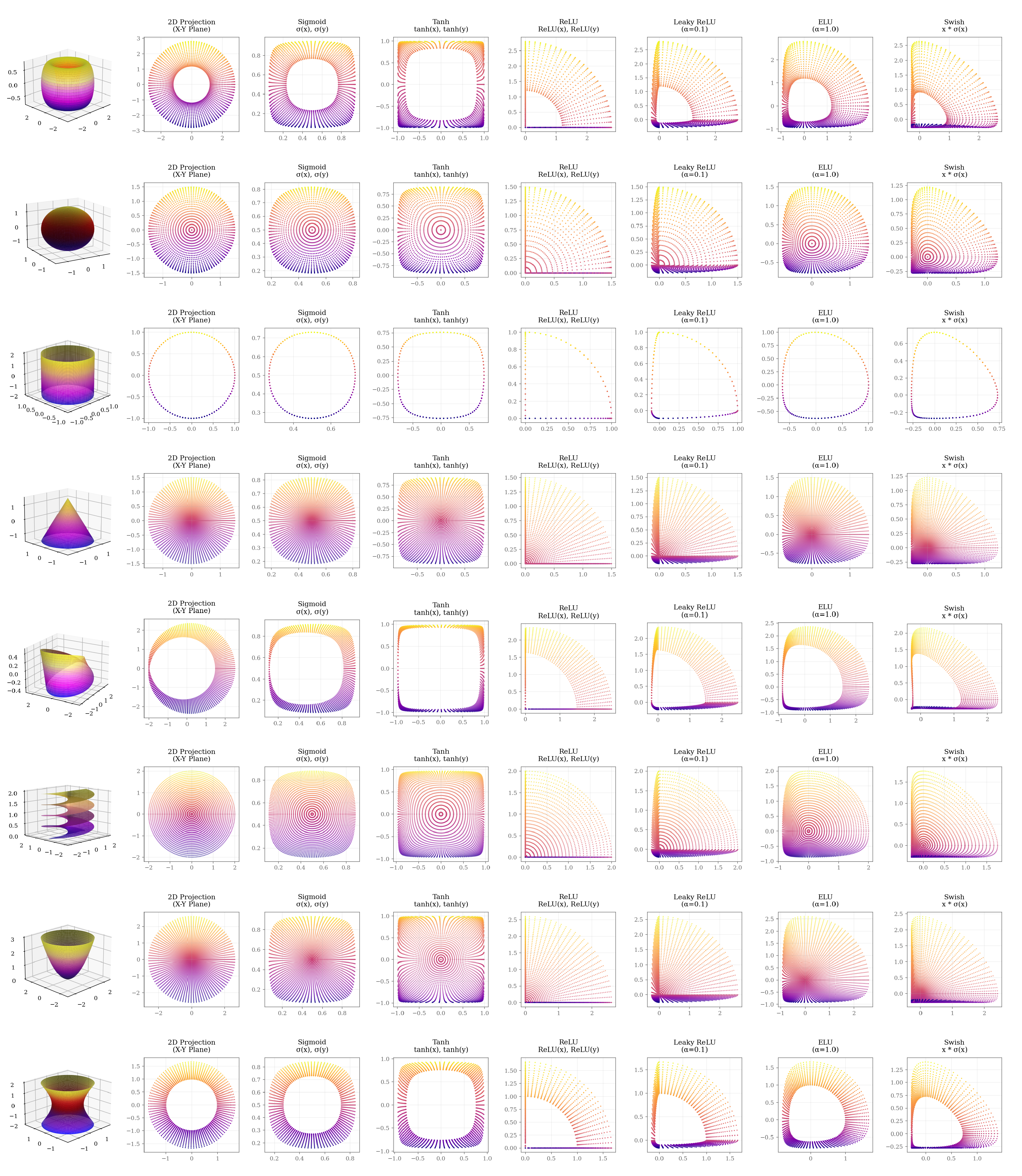
Figure 1.
Illustration of how non-linear activation functions can distort the geometric structure of the input data manifold, leading to potential information loss. The original manifold (left) is transformed into a distorted representation after applying a non-linear activation functions.
Figure 1.
Illustration of how non-linear activation functions can distort the geometric structure of the input data manifold, leading to potential information loss. The original manifold (left) is transformed into a distorted representation after applying a non-linear activation functions.
While these distortions are precisely what grant neural networks their expressive power to warp the feature space and create complex decision boundaries, they come at the cost of potentially discarding information present in the original geometric configuration of the data. The network learns which information to preserve and which to discard based on the optimization objective, but the mechanism relies on potentially non-smooth or non-injective transformations introduced by . This highlights the conflation of magnitude and direction in the dot product, the information loss from activation functions, and the lack of a unified measure for proximity and alignment, setting the stage for the Yat-product.
3. Methodology: A Framework for Geometry-Aware Computation
3.1. The Yat-Product: A Unified Operator for Alignment and Proximity
The methodological innovations presented in this work are fundamentally rooted in the Yat-product, introduced in Section 1. This single operator serves as the foundation for subsequent layers and networks.
The Yat-product is formally defined as [19,20]. It exhibits a unique form of non-linearity. Unlike conventional activation functions (e.g., ReLU, sigmoid) which are often applied as separate, somewhat heuristic, transformations to introduce non-linearity after a linear operation, the non-linearity in the Yat-product arises directly from its mathematical structure. It is a function of the squared dot product (capturing alignment) and the inverse squared Euclidean distance (capturing proximity) between the weight vector and the input vector . This formulation provides a rich, explainable non-linearity based on fundamental geometric and algebraic relationships, rather than an imposed, "artificial" non-linear mapping. The interaction between the numerator and the denominator allows for complex responses that are inherently tied to the geometric interplay of the input vectors.
As visualized in Figure 2, the Yat-product creates a potential well around the weight vector , reflecting both alignment and proximity.
3.2. Comparison to Standard Similarity and Distance Metrics
To further appreciate the unique characteristics of the Yat-product, it is instructive to compare it with other common similarity or distance metrics [13,14,23,24]:
- Dot Product (): The dot product measures the projection of one vector onto another, thus capturing both alignment and magnitude. A larger magnitude in either vector, even with constant alignment, leads to a larger dot product. While useful, its direct sensitivity to magnitude can sometimes overshadow the pure geometric alignment.
- Cosine Similarity (): Cosine similarity normalizes the dot product by the magnitudes of the vectors, yielding the cosine of the angle between them. This makes it purely a measure of alignment, insensitive to vector magnitudes. However, as pointed out, this means it loses information about true distance or scale; two vectors can have perfect cosine similarity (e.g., value of 1) even if one is very distant from the other, as long as they point in the same direction.
- Euclidean Distance (): This metric computes the straight-line distance between the endpoints of two vectors. It is a direct measure of proximity. However, it does not inherently capture alignment. For instance, if is a reference vector, all vectors lying on the surface of a hypersphere centered at will have the same Euclidean distance to , regardless of their orientation relative to .
- Yat-Product (): The Yat-product uniquely combines aspects of both alignment and proximity in a non-linear fashion. The numerator, , emphasizes strong alignment (being maximal when vectors are collinear and zero when orthogonal) and is sensitive to magnitude. The denominator, , heavily penalizes large distances between and . This synergy allows the Yat-product to be highly selective. It seeks points that are not only well-aligned with the weight vector but also close to it. Unlike cosine similarity, it distinguishes between aligned vectors at different distances. Unlike Euclidean distance alone, it differentiates based on orientation. This combined sensitivity allows the Yat-product to identify matches with a high degree of specificity, akin to locating a point with "atomic level" precision, as it requires both conditions (alignment and proximity) to be met strongly for a high output.
Beyond its geometric interpretation, the Yat-product has a profound connection to information theory when its arguments are probability distributions [25,26,27] (see Appendix G.7 for formal results). In this context, it can be viewed as a signal-to-noise ratio, where the "signal" measures distributional alignment and the "noise" quantifies their dissimilarity.
The Yat-product’s ability to discern between aligned vectors at varying distances, as well as its sensitivity to the angle between vectors, is illustrated in Figure 2 and Figure 3. The vector field generated by the Yat-product can be visualized as a potential well around the weight vector , where the strength of the interaction diminishes with distance, akin to gravitational or electrostatic fields. This visualization underscores how the Yat-product captures both alignment and proximity in a unified manner. This combined sensitivity is crucial for tasks where both the orientation and the relative position of features are important.
3.3. Design Philosophy: Intrinsic Non-Linearity and Self-Regulation
A central hypothesis underpinning our methodological choices is that the Yat-product (Section 1) possesses inherent non-linearity and self-regulating properties that can reduce or eliminate the need for conventional activation functions (e.g., ReLU, sigmoid, GeLU) and normalization layers (e.g., Batch Normalization, Layer Normalization).
This philosophy recontextualizes the fundamental components of neural computation. Neuron weights () and input signals () are not merely operands in a linear transformation followed by a non-linear activation; instead, they are conceptualized as co-equal vector entities inhabiting a shared, high-dimensional feature manifold. Within this framework, each vector can be viewed as an analogue to a fundamental particle or feature vector, with its constituent dimensions potentially encoding excitatory, inhibitory, or neutral characteristics relative to other entities in the space. The Yat-product (Section 1) then transcends simple similarity assessment; it functions as a sophisticated interaction potential, , quantifying the ’field effects’ between these vector entities. This interaction is reminiscent of n-body problems in physics. In machine learning, it draws parallels with, yet distinctively evolves from, learned metric spaces in contrastive learning, particularly those employing a triplet loss framework. While triplet loss aims to pull positive pairs closer and push negative pairs apart in the embedding space, our Yat-product seeks a more nuanced relationship: ’positive’ interactions (high Yat-product value) require both strong alignment (high ) and close proximity (low ). Conversely, ’negative’ or dissimilar relationships are not merely represented by distance, but more significantly by orthogonality (leading to a vanishing numerator), which signifies a form of linear independence and contributes to the system’s capacity for true non-linear discrimination. Crucially, the non-linearity required for complex pattern recognition is not an external imposition (e.g., via a separate activation function) but is intrinsic to this interaction potential. The interplay between the squared dot product (alignment sensitivity) and the inverse squared Euclidean distance (proximity sensitivity) in its formulation directly sculpts a complex, non-linear response landscape without recourse to auxiliary functions.
Furthermore, this conceptualization of the Yat-product as an intrinsic interaction potential suggests inherent self-regulating properties. The distance-sensitive denominator, , acts as a natural dampening mechanism. As the ’distance’ (dissimilarity in terms of position) between interacting vector entities and increases, the strength of their interaction, and thus the resultant activation, diminishes quadratically. This behavior is hypothesized to inherently curtail runaway activations and stabilize learning dynamics by ensuring that responses are localized and bounded. Such intrinsic stabilization contrasts sharply with conventional approaches that rely on explicit normalization layers (e.g., Batch Normalization, Layer Normalization) to manage activation statistics post-hoc. These layers, while effective, introduce additional computational overhead, can obscure direct input-output relationships, and sometimes complicate the theoretical analysis of network behavior. The Yat-product’s formulation, therefore, offers a pathway to architectures where regulatory mechanisms are embedded within the primary computational fabric of the network.
The inherent non-linearity of the Yat-product, coupled with the self-regulating properties suggested by its formulation (and formally proven in Appendix G.3), are central to our hypothesis that it can form the basis of powerful and robust neural architectures. These intrinsic characteristics open avenues for simplifying network design, potentially reducing reliance on or even eliminating conventional activation functions and normalization layers.
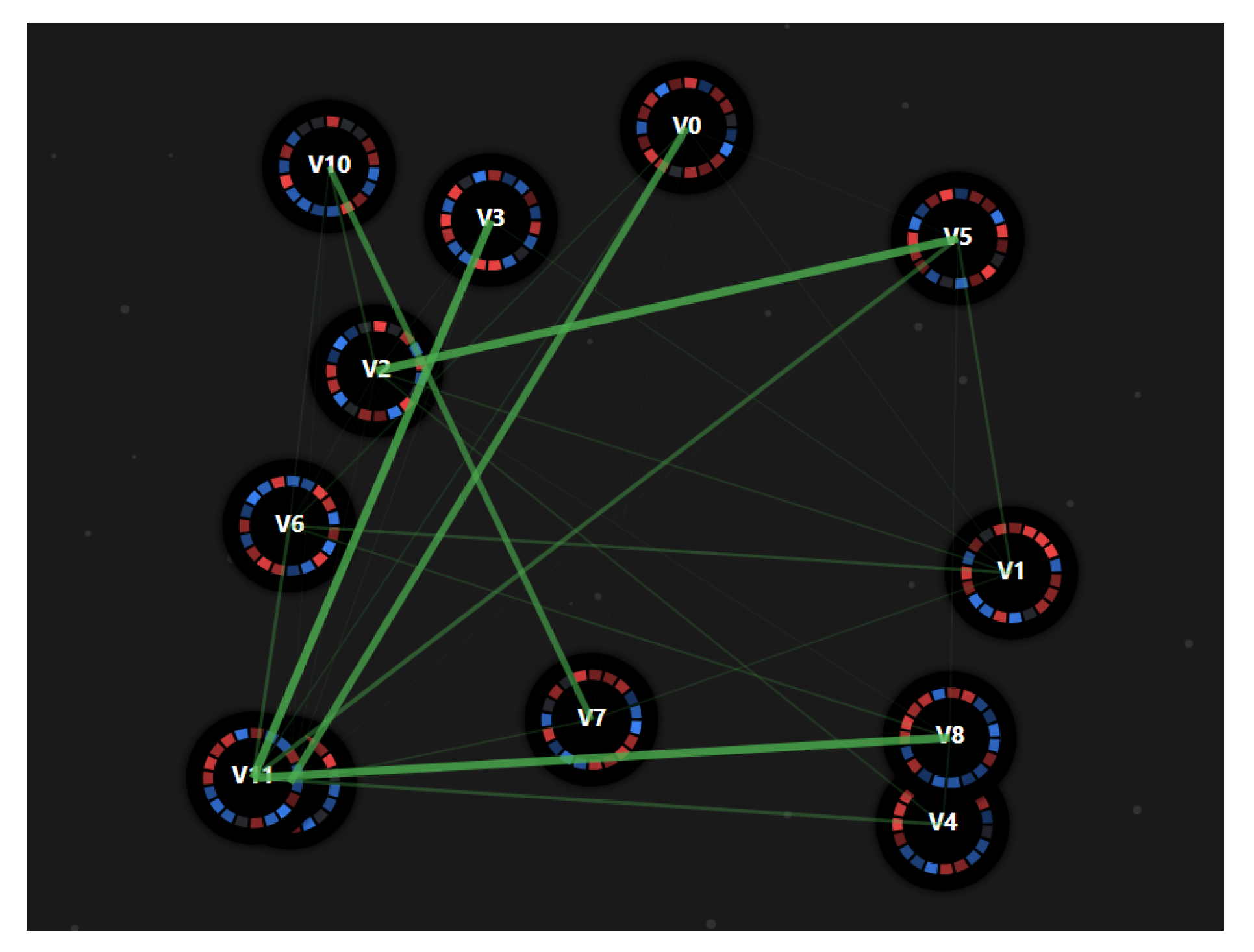
Figure 4.
The Vectoverse: Conceptualizing neural computation where weight vectors () and input vectors () are akin to fundamental particles (vectoms). The interaction force between them is quantified by the Yat-product, which measures their alignment and proximity, defining a field of influence.
Figure 4.
The Vectoverse: Conceptualizing neural computation where weight vectors () and input vectors () are akin to fundamental particles (vectoms). The interaction force between them is quantified by the Yat-product, which measures their alignment and proximity, defining a field of influence.
3.4. Core Building Blocks
Now, we show how the Yat-product is operationalized into reusable layers.
3.4.1. The Neural Matter Network (NMN) Layer
The first and simplest application of the Yat-product is in Neural-Matter Network (NMN) layers. These networks represent a departure from traditional Multi-Layer Perceptrons (MLPs) by employing the non-linear, spatially-aware -kernel (derived from the Yat-product, see Section 3.1) as the primary interaction mechanism, instead of the conventional linear projection ().
An NMN layer transforms an input vector () into an output (here, we consider a scalar output h for simplicity, extendable to vector outputs by aggregating the influence of multiple "neural matter" units). Each unit i is defined by a weight vector () (acting as a positional anchor or prototype) and a bias term (). The layer output is computed as:
where:
- is the weight vector of the i-th NMN unit.
- is the bias term for the i-th NMN unit.
- represents the Yat-product between the weight vector and the input .
- n is the number of NMN units in the layer.
- s is a scaling factor.
This formulation allows each NMN unit to respond based on both alignment and proximity to its learned weight vector.
A key theoretical guarantee for NMNs is their capacity for universal function approximation [3,4,21,22,28,29]. This is significant because, unlike traditional neural networks that depend on separate, often heuristically chosen, activation functions (e.g., ReLU, sigmoid) to introduce non-linearity, the approximation power of NMNs is an intrinsic property of the -kernel itself. This finding validates the Yat-product as a self-contained computational primitive powerful enough to form the basis of expressive neural architectures, distinguishing NMNs from classical MLP-based designs and supporting our core hypothesis that effective, geometry-aware computation is possible without separate activation functions [10,11,12].
3.4.2. Convolutional Neural-Matter Networks (CNMNs) and the Yat-Convolution Layer
To extend the principles of Neural-Matter Networks (NMNs) (Section 3.4.1) and the Yat-product (Section 1) to spatially structured data like images, we introduce the Yat-Convolution (Yat-Conv) layer. This layer adapts the Yat-product to operate on local receptive fields, analogous to standard convolutional layers. The Yat-Conv operation is defined as:
where K is the convolutional kernel and is the input patch at location corresponding to the receptive field of the kernel.
3.4.3. The Yat-Attention Mechanism
To extend the Yat-product’s application to sequence modeling, we propose the Yat-Attention mechanism. This mechanism serves as an alternative to the standard scaled dot-product attention found in transformer architectures by replacing the dot product used for calculating query-key similarity with the Yat-product (Section 3.1). Given Query (Q), Key (K), and Value (V) matrices, Yat-Attention is computed as:
where the operation signifies applying the Yat-product element-wise between query and key vectors (e.g., the -th element is ), and s is a scaling factor.
3.5. Architectural Implementations
The development of architectures like AetherResNet and AetherGPT without standard components (like separate activation and normalization layers) is a deliberate effort to test the hypothesis outlined in Section 3.3. Key architectural distinctions driven by this philosophy include:
- Feed-Forward Networks (FFNs): The FFNs within are constructed using NMN layers (Section 3.4.1) without explicit non-linear activation functions.
- Omission of Standard Layers: Consistent with this design philosophy, explicit activation functions and standard normalization layers are intentionally omitted.
Additionally, in all NMN-based architectures, we use a scaling factor , where n is the number of NMN units and is a learnable parameter. This scaling is designed to adaptively control the overall magnitude of the layer outputs as a function of network width.
By minimizing reliance on these traditional layers, we aim to explore simpler, potentially more efficient, and interpretable models where the primary computational operator itself handles these crucial aspects of neural processing. Furthermore, this principle of substituting the dot product with the Yat-product is not limited to the architectures presented and holds potential for enhancing other neural network paradigms.
3.5.1. Convolutional NMNs:
AetherResNet is a Convolutional Neural-Matter Network (CNMN) built by replacing all standard convolutions in a ResNet18 architecture with the Yat-Conv layers. Building upon the Yat-Conv layer, CNMNs adapt conventional convolutional architectures by employing the Yat-Conv layer as the primary feature extraction mechanism. The core idea is to leverage the geometric sensitivity and inherent non-linearity of the Yat-product within deep convolutional frameworks. Consistent with the philosophy of Section 3.3, AetherResNet omits Batch Normalization and activation functions [9,30,31,32]. The design relies on the hypothesis that the Yat-product itself provides sufficient non-linearity and a degree of self-regulation.
In each CNMN residual block, we use a YatConv layer (with input dimension n and output dimension m) followed by a linear Conv layer (with input and output dimension m), without any activation functions or normalization layers (see Figure A15).
3.5.2. YatFormer: AetherGPT
AetherGPT is a YatFormer model that uses Yat-Attention (from Section 3.4.3) for sequence interaction and NMN layers (from Section 3.4.1) in its feed-forward blocks. Building upon the Yat-Attention mechanism, which forms its cornerstone, we introduce YatFormer, a family of transformer-based models. As a specific instantiation for our investigations, we developed AetherGPT. This model adapts the architectural principles of GPT-2. Again, following the philosophy of Section 3.3, it omits standard normalization and activation layers.
In YatFormer/AetherGPT, we remove the projection layer after the attention mechanism, as the dot product between the attention map and the value matrix V already serves as a linear projection (see Fig. A16). Furthermore, in the MLP block, we do not multiply the first layer’s width by 4 as in standard transformers. Instead, we use a YatNMN layer with input and output dimensions equal to the embedding dimension, followed by a linear layer, also with input and output dimensions equal to the embedding dimension (see Fig. A17).
3.6. Output Processing for Non-Negative Scores
The Yat-product and its derivatives, such as the -kernel, naturally yield non-negative scores. In many machine learning contexts, particularly when these scores need to be interpreted as probabilities, attention weights, or simply normalized outputs, it is essential to apply a squashing function to map them to a desired range (e.g., [0, 1] or ensuring a set of scores sum to 1).
Squashing functions for non-negative scores can be broadly categorized into two types:
- Competitive (Vector-Normalizing) Functions: These functions normalize a set of scores collectively, producing a distribution over the vector. Each output depends on the values of all dimensions, allowing for competitive interactions among them. This is useful for attention mechanisms or probability assignments where the sum of outputs is meaningful.
- Individualistic (Per-Dimension) Functions: These functions squash each score independently, without reference to other values in the vector. Each output depends only on its corresponding input, making them suitable for bounding or interpreting individual activations.
Traditional squashing functions, however, present challenges when applied to non-negative inputs:
- Standard Sigmoid Function (): When applied to non-negative inputs (), the standard sigmoid function produces outputs in the range . The minimum value of for renders it unsuitable for scenarios where small non-negative scores should map to values close to 0.
- Standard Softmax Function (): The use of the exponential function in softmax can lead to hard distributions, where one input value significantly dominates the output, pushing other probabilities very close to zero. While this is often desired for classification, it can be too aggressive if a softer assignment of probabilities or attention is preferred. Additionally, softmax can suffer from numerical instability for large input values due to the exponentials.
Given these limitations and the non-negative nature of Yat-product scores, we consider alternative squashing functions more suited to this domain:
-
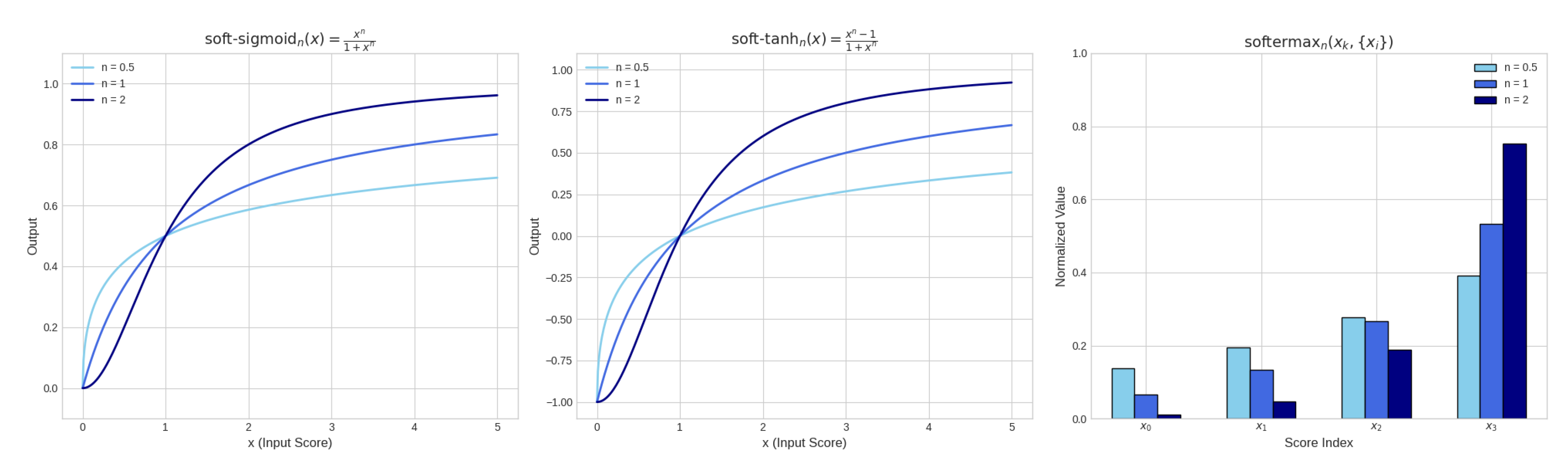
softermax (Competitive): This function normalizes a score (optionally raised to a power ) relative to the sum of a set of non-negative scores (each raised to n), with a small constant for numerical stability. It is defined as:Unlike softmax, softermax does not use exponentials, which avoids numerical instability for large inputs and provides a more direct, interpretable translation of the underlying scores into a normalized distribution. The power n controls the sharpness of the distribution: recovers the original Softermax, while makes the distribution harder (more peaked), and makes it softer.
-
soft-sigmoid (Individualistic): This function squashes a single non-negative score (optionally raised to a power ) into the range . It is defined as:The power n modulates the softness: higher n makes the function approach zero faster for large x, while makes the decay slower.
-
soft-tanh (Individualistic): This function maps a non-negative score (optionally raised to a power ) to the range by linearly transforming the output of soft-sigmoid. It is defined as:The power n again controls the transition sharpness: higher n makes the function approach more quickly for large x.
Figure 5.
Visualization of the softermax, soft-sigmoid, and soft-tanh functions. These functions are designed to handle non-negative inputs from the Yat-product and its derivatives, providing appropriate squashing mechanisms that maintain sensitivity across the range of non-negative inputs.
Figure 5.
Visualization of the softermax, soft-sigmoid, and soft-tanh functions. These functions are designed to handle non-negative inputs from the Yat-product and its derivatives, providing appropriate squashing mechanisms that maintain sensitivity across the range of non-negative inputs.
These functions are particularly well-suited for the outputs of Yat-product-based computations, as they maintain sensitivity across the range of non-negative inputs while avoiding the pitfalls of standard activation functions [7,8,9].
The main role of these squashing functions can be categorized into two main categories:
- Collective Communication and Space Splitting: The softermax function allows for a comparative analysis of scores, reflecting their orthogonality and spatial proximity to an input vector. A higher score indicates that a vector is more aligned and closer to the input, while a lower score suggests greater orthogonality. This facilitates a competitive interaction where vectors vie for influence based on their geometric relationship with the input. The power parameter n, analogous to the temperature in softmax, controls the sharpness of the gravitational potential well’s slope.
- Individual Score Squashing: The soft-sigmoid and soft-tanh functions are used to squash individual non-negative scores into a bounded range, typically for soft-sigmoid and for soft-tanh. They are particularly useful when the output needs to be interpreted as a probability or when a bounded response is required, as each score is processed independently of the others. The power parameter controls the steepness of the function, while the minimum value can be interpreted as an orthogonality score.
3.7. Mathematical Guarantees of the Yat-Product and NMNs
The Yat-product and the resulting Neural-Matter Networks (NMNs) are supported by several key mathematical properties, each formally proven in the appendices:
- Mercer Kernel Property: The Yat-product is a symmetric, positive semi-definite Mercer kernel, enabling its use in kernel-based learning methods (see Appendix G.2).
- Universal Approximation: NMNs with Yat-product activations can approximate any continuous function on a compact set, establishing their expressive power (see Appendix G.6).
- Self-Regulation: The output of a Yat-product neuron is naturally bounded and converges to a finite value as input magnitude increases, ensuring stable activations (see Appendix G.3).
- Stable Gradient: The gradient of the Yat-product with respect to its input vanishes for distant inputs, preventing large, destabilizing updates from outliers (see Appendix G.5).
- Information-Theoretic Duality: The Yat-product unifies geometric and information-theoretic notions of similarity and orthogonality, with formal theorems connecting it to KL divergence and cross-entropy (see Appendix G.7).
4. Results and Discussion
The Yat-product’s non-linearity is not merely a mathematical curiosity; it has practical implications for neural computation. By integrating alignment and proximity into a single operator, the Yat-product allows for more nuanced feature learning. It can adaptively respond to inputs based on their geometric relationships with learned weight vectors, enabling the network to capture complex patterns without the need for separate activation functions.
Consider the classic XOR problem, which is not linearly separable and thus cannot be solved by a single traditional neuron (linear perceptron). The inputs are , , , and . A single Yat-product unit can, however, solve this. Let the weight vector be .
For : , so .
For : , so .
For : . . So .
For : . . So .
Thus, the Yat-product unit with an appropriate weight vector (such as one where components have opposite signs, reflecting the XOR logic) naturally separates the XOR patterns, effectively acting as a mathematical kernel. We have formally proven that the Yat-product is a valid Mercer kernel in Appendix G.2 [33,34,35,36,37,38].
To understand its behavior during learning, we analyze its gradient. A key property for stable training is that the gradient with respect to the input, , diminishes as the input moves far from the weight vector . This ensures that distant outliers do not cause large, destabilizing updates. We have formally proven this property in Appendix G.5, demonstrating that .
The presence of in the denominator ensures that the derivative remains well-defined, avoiding division by zero and contributing to numerical stability. This contrasts with activation functions like ReLU, which have a derivative of zero for negative inputs, potentially leading to "dead neurons." The smooth and generally non-zero gradient of the Yat-product is hypothesized to contribute to more stable and efficient learning dynamics, reducing the reliance on auxiliary mechanisms like complex normalization schemes. The non-linearity is thus not an add-on but an intrinsic property derived from the direct mathematical interaction of vector projection (alignment, via the term) and vector distance (proximity, via the term). This provides a mathematically grounded basis for feature learning, as the unit becomes selectively responsive to inputs that exhibit specific geometric relationships, both in terms of angular alignment and spatial proximity, to its learned weight vector . Consequently, can be interpreted as a learned feature template or prototype that the unit is tuned to detect, with the Yat-product quantifying the degree of match in a nuanced, non-linear fashion.
The gradient of the Yat-product, being responsive across the input space, actively pushes the neuron’s weights away from configurations that would lead to a zero output (neuron death, e.g., at an input of for this problem if weights were also near zero). This contrasts with a simple dot product neuron where the gradient might vanish or lead to a global minimum at zero output for certain problems. For instance, when considering gradient-based optimization, the loss landscape "seen" by the Yat-product neuron in the XOR context would exhibit a peak or high loss at (if that were the target for non-zero outputs), encouraging weights to move towards a state that correctly classifies. Conversely, a simple dot product neuron might present a loss landscape where a gradient-based optimizer could find a stable (but incorrect) minimum at zero output. This ability to avoid such dead zones and actively shape the decision boundary makes it helpful to solve problems like XOR with a single unit, leveraging its inherent non-linearity as a mathematical kernel.
Figure 6.
Comparison of the loss landscape for a simple dot product neuron and a Yat-product neuron. The dot product neuron has a stable minimum at zero output which doesn’t solve the xor problem and cause the neuron death, while the Yat-product neuron resides in a valley of orthogonality, allowing it to avoid dead zones and actively shape the decision boundary. This illustrates the Yat-product’s ability to solve problems like XOR with a single unit, leveraging its inherent non-linearity as a mathematical kernel.
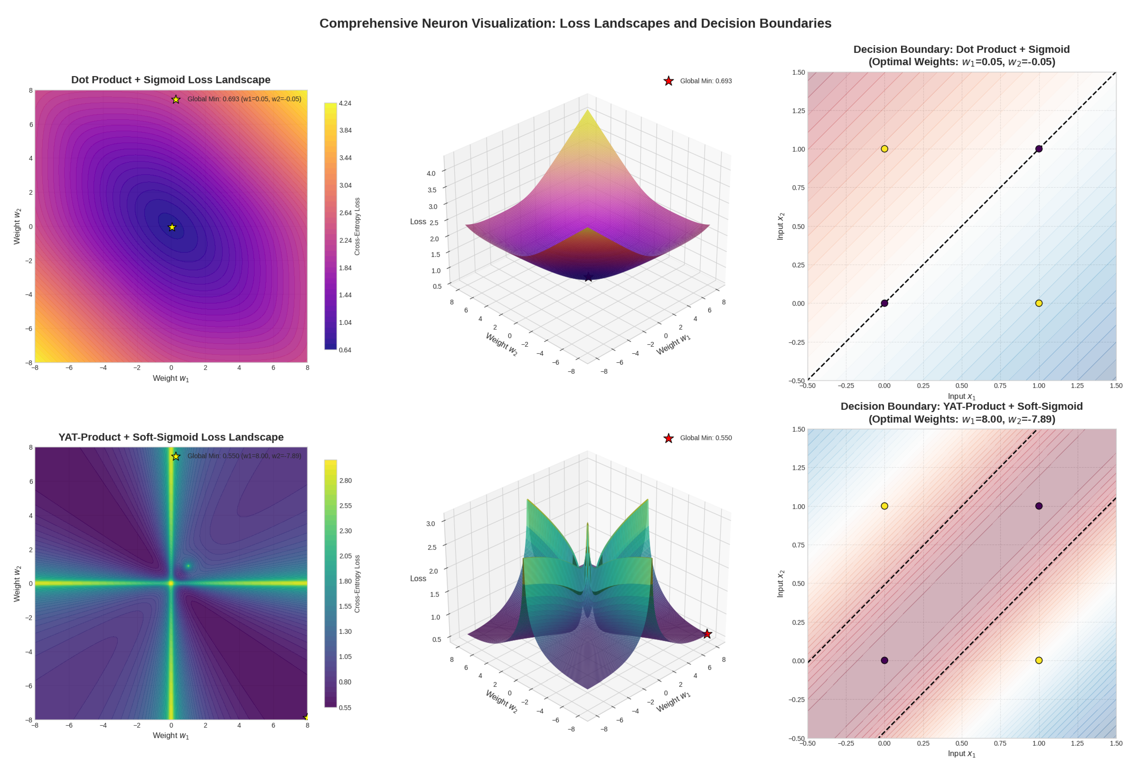
Conceptually, the decision boundary or vector field generated by a simple dot product neuron is linear, forming a hyperplane that attempts to separate data points. In contrast, the Yat-product generates a more complex, non-linear vector field. This field can be visualized as creating a series of potential wells or peaks centered around the weight vector , with the strength of influence decaying with distance. The condition defines a "valley" of zero output where vectors are orthogonal to the weight vector. This structure allows for more nuanced and localized responses, akin to a superposition of influences rather than a single linear division, enabling the capture of intricate patterns in the data.
4.1. Your Neuron is a secret Vortex
We begin by analyzing the fundamental learning dynamics that emerge in both conventional and our proposed architectures. In artificial intelligence, competitive learning manifests in various forms, whether through linear classification using dot products or clustering using Euclidean distances. Both approaches involve partitioning the feature space between neurons, which can be conceptualized as prototype learning where each neuron claims a territorial “field” in the representation space.
Figure 7.
Comparison of decision boundaries formed by a conventional linear model (left) and our proposed Yat-product method (right). The conventional model’s prototypes grow unbounded, while our method learns more representative prototypes that better capture class distributions.
Figure 7.
Comparison of decision boundaries formed by a conventional linear model (left) and our proposed Yat-product method (right). The conventional model’s prototypes grow unbounded, while our method learns more representative prototypes that better capture class distributions.
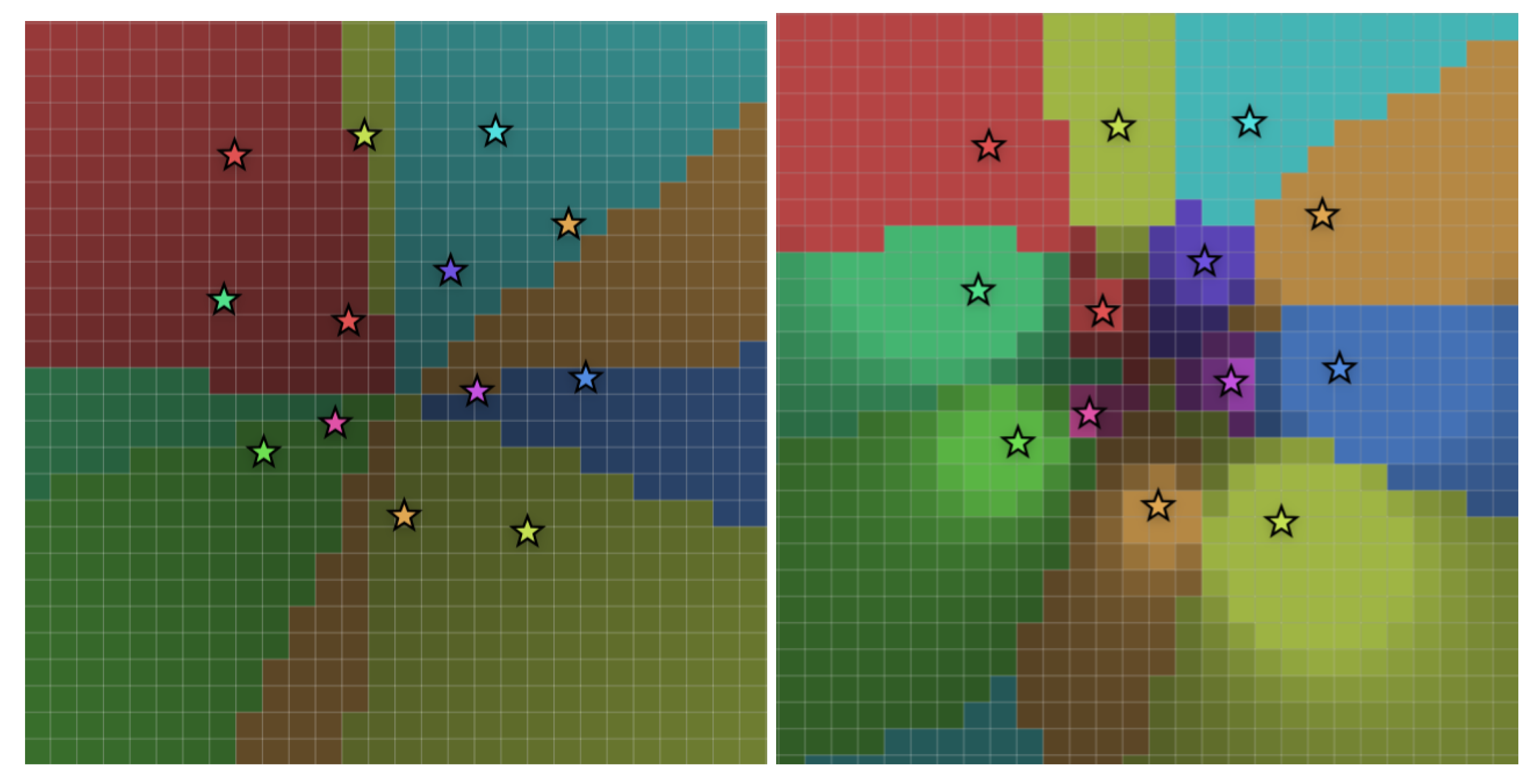
In this experiment, we analyze the learning dynamics of a linear model on a synthetic dataset, comparing the formation of decision boundaries by conventional neurons employing standard dot products with those generated by our proposed Yat-product method.
In a conventional linear model, the logit for each class i is computed as:
where is the weight vector (prototype) for class i, and is the input vector. The softmax function then normalizes these logits into probabilities:
The decision boundary between any two classes i and j forms a linear hyperplane defined by:
During training via gradient descent, each prototype is updated to maximize its alignment with the data distributions of its assigned class. This optimization process often leads to an unbounded increase in prototype magnitudes, as directly amplifies the logit , thereby increasing the model’s confidence. However, the decision boundaries themselves remain linear hyperplanes, creating rigid geometric separations in the feature space.
In contrast, the non-linear Yat-product allows neurons to learn more representative prototypes for each class, leading to the formation of more nuanced decision boundaries. For the Yat-product, the response of neuron i to input is given by:
This formulation embodies the signal-to-noise ratio interpretation established in our theoretical framework (Appendix G.7), where the squared dot product represents the "signal" of distributional alignment, and quantifies the "noise" of dissimilarity. The Yat-product thus provides a principled geometric measure that balances similarity and proximity in a theoretically grounded manner.
Similarly to conventional neurons, the Yat-product outputs are normalized using the softmax function:
This softmax normalization serves a crucial role in the competitive dynamics of Yat-product neurons. The softmax function acts as a transformation that maps from the real-valued Yat-product responses to a delta distribution in probability space. This softmax distribution over Yat-product scores can be interpreted as the posterior responsibility of each prototype (neuron) for the input, drawing a direct connection to Gaussian Mixture Models (GMMs) and expectation-maximization frameworks.
The softmax can also be viewed as computing a categorical distribution proportional to exponentiated log-likelihoods, which in this case derive from a geometric Yat-product similarity rather than traditional probabilistic assumptions. This bridges the gap between probabilistic views (such as EM algorithms and classification) and our geometric formulation, providing a principled foundation for the competitive dynamics.
As training progresses and the differences between Yat-product responses become more pronounced, the softmax transformation approaches a delta distribution, where the winning neuron (with the highest Yat-product response) approaches probability 1 while all others approach 0. This winner-take-all mechanism enables competitive learning dynamics where each neuron competes to "take over" regions of the input space based on their vortex-like attraction fields.
The decision boundary between two neurons with prototypes and is defined by the condition where their responses are equal:
Expanding this condition:
Cross-multiplying and rearranging:
This equation defines a complex, non-linear decision boundary that depends on both the alignment (through the squared dot products) and the proximity (through the squared distances) between the input and each prototype. Unlike the linear hyperplane formed by conventional dot product neurons, the Yat-product creates what we term a vortex phenomenon or gravitational potential well around each prototype.
The space partitioning behavior of the Yat-product exhibits several key properties that create this vortex-like effect:
- Gravitational Attraction: The inverse-square relationship in the denominator creates a field where points are more strongly attracted to nearby prototypes, similar to gravitational fields in physics.
- Alignment Amplification: The squared dot product in the numerator creates a strong response for well-aligned inputs, while the vortex effect pulls data points toward the prototype center.
- Bounded Potential Wells: Each neuron creates a localized potential well with bounded depth, preventing the unbounded growth seen in linear neurons. This boundedness is theoretically guaranteed by the Minimal and Maximal Similarity Characterizations (Theorems A7 and A8), which establish that with well-defined extremal conditions.
- Curved Decision Boundaries: The resulting decision boundaries are non-linear curves that wrap around the data distribution, creating vortex-like territorial regions for each neuron.
This vortex phenomenon allows each Yat-product neuron to create a territorial "field" in the representation space, where data points are pulled toward the dominant prototype based on both similarity and proximity metrics. The field each neuron occupies can indeed be considered a vortex, where the strength of attraction follows an inverse-square law, creating more natural and geometrically faithful decision boundaries.
The combination of the Yat-product’s vortex-like attraction and the softmax’s competitive normalization creates a powerful space partitioning mechanism. Each neuron’s vortex field competes with others through the softmax transformation, and the neuron with the strongest local attraction (highest Yat-product response) wins that region. Over time, this leads to a natural tessellation of the input space, where each neuron’s territory is defined by the regions where its vortex field dominates. The softmax transformation (where is the -dimensional probability simplex) ensures that these territorial boundaries are sharp and well-defined, transforming the continuous real-valued responses into discrete delta distributions that clearly assign each input to its dominant neuron.
Orthogonality and Competitive Dynamics: The competitive learning behavior observed in practice is theoretically grounded in our Orthogonality-Entropy Connection. When two prototypes and develop disjoint support regions, they become Euclidean orthogonal (), which corresponds to:
This geometric-probabilistic duality explains why neurons naturally develop specialized, non-overlapping representations during competitive learning. The infinite cross-entropy between orthogonal prototypes creates strong pressure for territorial separation, preventing the collapse to identical representations that can plague conventional competitive learning systems.
These prototypes are optimized to maximize parallelism and minimize distance to all points within their class distribution. When minimizing distance becomes challenging, the properties of the Yat-product enable the prototype to exist in a superposition state, prioritizing the maximization of parallelism over strict distance minimization.
4.2. Do you even MNIST bro?
Having established the theoretical foundation of the vortex phenomenon in Section 4.1, we now validate these insights on the canonical MNIST dataset. This experiment serves as a bridge between our geometric theory and practical applications, demonstrating how the vortex-like territorial dynamics translate into improved prototype learning on real data.
In our MNIST experiments, the network consists of neurons, each corresponding to one of the digit classes (0–9). Each neuron’s prototype is represented as a vector , where . The input images are obtained by flattening the original pixel images, so each neuron’s prototype has the same dimensionality as the input, i.e., . This structure allows each neuron to learn class-specific features in the full image space.
The MNIST dataset provides an ideal testbed for examining the vortex phenomenon because its 10-class structure allows clear visualization of how different neurons compete for territorial control in the feature space. We specifically investigate whether the bounded attraction fields and territorial partitioning predicted by our theory manifest as improved prototype quality and learning dynamics in practice.
Experimental Design: We train both conventional linear classifiers and our Yat-product networks on MNIST, analyzing three key aspects that directly relate to the vortex phenomenon:
- Prototype Evolution Dynamics: How do prototypes evolve during training under different competitive mechanisms?
- Territorial Boundary Formation: Do we observe the predicted non-linear decision boundaries and vortex-like attraction fields?
- Representational Quality: How does the theoretical prediction of bounded, concentrated prototypes translate to interpretability?
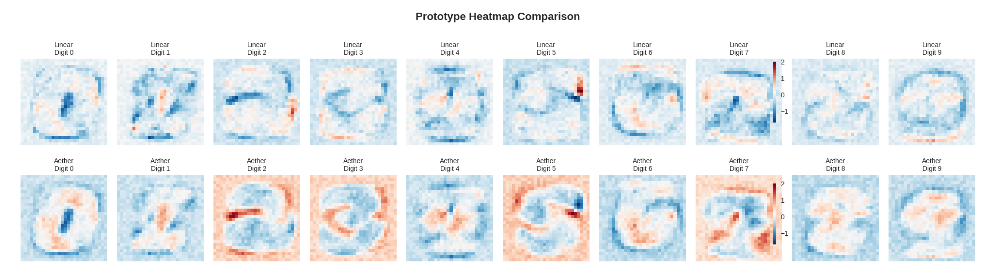
The prototype evolution during training reveals the fundamental differences between conventional unbounded growth and our bounded vortex dynamics. Figure 9 shows the final learned prototypes, providing striking empirical confirmation of our vortex theory. The conventional linear model produces prototypes that exhibit the unbounded growth predicted by our analysis—these prototypes become increasingly diffuse and less interpretable as they grow to maximize margin separation. The resulting digit representations are blurry and lack the fine-grained features necessary for robust classification.
In stark contrast, the Yat-product method produces prototypes that perfectly exemplify the bounded vortex fields described in our theory. Each digit prototype exhibits:
- Localized Concentration: Sharp, well-defined features that correspond to the bounded potential wells predicted by our Minimal and Maximal Similarity Characterizations (Theorems A7 and A8)
- Class-Specific Territorial Structure: Each prototype captures unique digit characteristics, reflecting the competitive territorial dynamics where each neuron’s vortex field dominates specific regions of the input space
- Geometric Fidelity: The prototypes maintain geometric coherence with actual digit structure, confirming that the signal-to-noise ratio optimization preserves meaningful visual patterns
Figure 8.
Prototypes learned by the conventional linear model (top) and our proposed Yat-product method (bottom) on the MNIST dataset. The prototypes from our method are more distinct and representative of the digit classes, capturing finer details and class-specific characteristics.
Figure 8.
Prototypes learned by the conventional linear model (top) and our proposed Yat-product method (bottom) on the MNIST dataset. The prototypes from our method are more distinct and representative of the digit classes, capturing finer details and class-specific characteristics.
Superposition and Prototype Inversion: A unique property of the Yat-product neuron is its ability to exist in a superposition state, which can be empirically demonstrated by inverting the learned prototype. Specifically, if is a learned prototype, we consider the effect of replacing with (i.e., multiplying by ) at test time, without any retraining. For a conventional dot product neuron, this operation flips the sign of the logit:
This sign flip causes the softmax output to assign high probability to the incorrect class, resulting in a dramatic drop in accuracy (from 93% to nearly 0% in our MNIST experiments).
In contrast, for the Yat-product neuron, the response is:
Multiplying by leaves the numerator unchanged, since and . The denominator is also unchanged, as , which is symmetric with respect to the data distribution. As a result, the Yat-product neuron’s accuracy remains nearly unchanged (dropping only slightly from 92% to 89%), demonstrating its robustness to prototype inversion and its ability to represent solutions in a superposition state.
This property allows the Yat-product neuron to yield two valid solutions to the same dataset without retraining, a phenomenon not observed in conventional dot product neurons. The table below summarizes the empirical results:

Table 1.
Test accuracy on MNIST before and after prototype inversion () for dot product and Yat-product (yat) neurons.
Table 1.
Test accuracy on MNIST before and after prototype inversion () for dot product and Yat-product (yat) neurons.
| Neuron Type | Original Prototype | Inverted Prototype () |
|---|---|---|
| Dot Product | 91.88% | ≈0.01% |
| Yat-Product (Yat) | 92.18% | 87.87% |
4.3. Aether-GPT2: The Last Unexplainable Language Model
To demonstrate the versatility of our approach beyond vision tasks, we implement Aether-GPT2, incorporating the Yat-product architecture into the GPT2 framework for language modeling. We compare the perplexity scores between our Aether-GPT2 and the standard GPT2 architecture across multiple text corpora.
The results in Table 2 demonstrate that Aether-GPT2 achieves a validation loss competitive with the standard GPT-2 baseline. While the loss is marginally higher, it is critical to note that Aether-GPT2 attains this performance despite its simplified design, which entirely omits dedicated activation functions and normalization layers. This outcome highlights a promising trade-off between raw performance and architectural simplicity, efficiency, and the inherent interpretability afforded by the Yat-product. These findings establish Aether-GPT2 as a successful proof-of-concept, suggesting that the Yat-product can serve as a viable alternative to conventional neural network components.
Figure 9.
Loss Curve over the 600m tokens from fineweb trained on Kaggle TPU v3, Linear model is using standard GPT2 achitecture.
Figure 9.
Loss Curve over the 600m tokens from fineweb trained on Kaggle TPU v3, Linear model is using standard GPT2 achitecture.
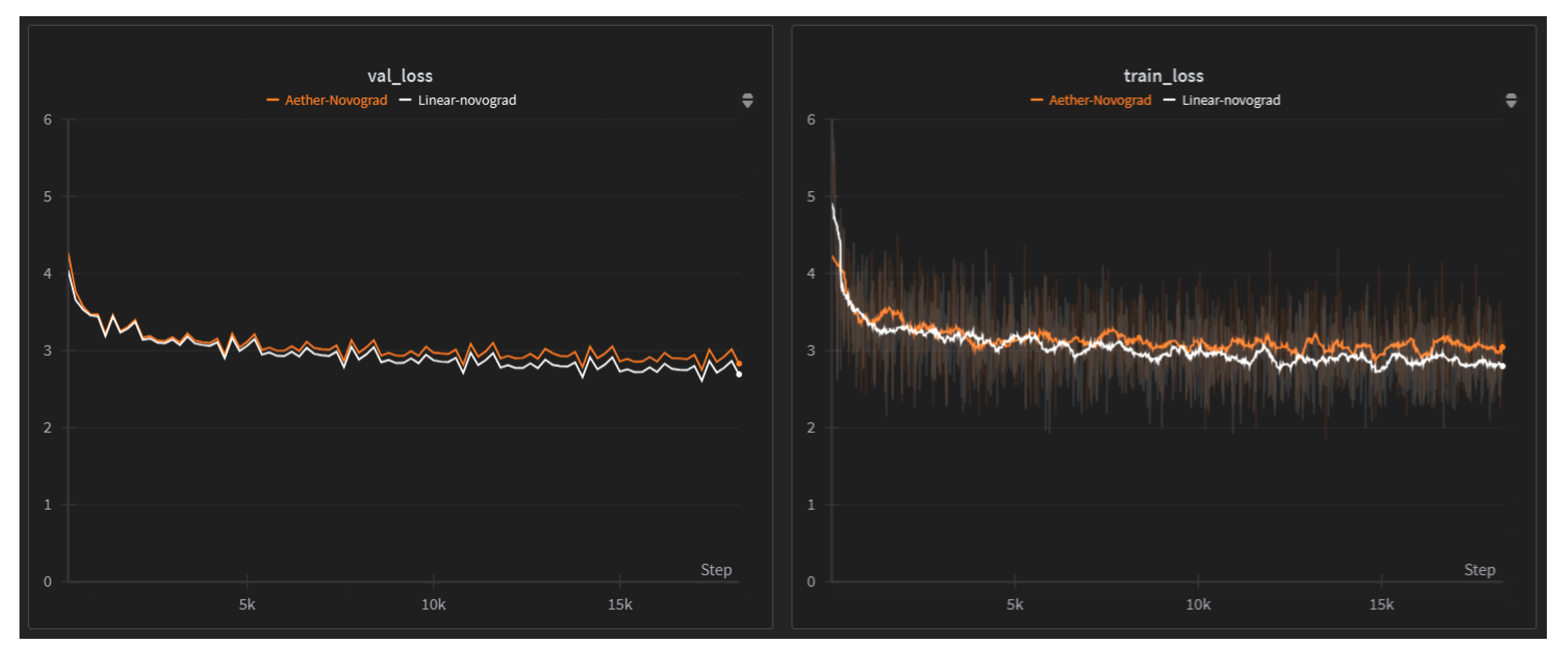
Table 3.
Aether-GPT2 Experiment Card
| Parameter | Value |
|---|---|
| Optimizer | Novograd |
| Learning Rate | 0.003 |
| Batch Size | 32 |
| Embedding Dimension | 768 |
| MLP Dimension | 768 (No x4) |
| Vocabulary Size | 50,257 |
| Number of Heads | 12 |
| Number of Blocks | 12 |
The results demonstrate that Aether-GPT2 consistently achieves close loss, indicating its ability to learn non-linearity without the need for activation functions.
The performance can be attributed to the Yat-product’s ability to capture more nuanced relationships between tokens, allowing the model to better understand contextual dependencies and semantic similarities in natural language.
5. Related Work
5.1. Inverse-Square Laws
The inverse-square law, where a quantity or intensity is inversely proportional to the square of the distance from its source, is a fundamental principle observed across numerous scientific disciplines [15]. This relationship signifies that as the distance from a source doubles, the intensity reduces to one-quarter of its original value.
In classical physics, this law is foundational. Newton’s Law of Universal Gravitation describes the force between two masses [16], and Coulomb’s Law defines the electrostatic force between charges [17]. The intensity of electromagnetic radiation, such as light, and the intensity of sound from a point source also diminish according to this principle. Gauss’s Law offers a unifying mathematical framework for these phenomena in fields like electromagnetism and gravitation, connecting them to the property that the divergence of such fields is zero outside the source [18]. Similarly, thermal radiation intensity from a point source adheres to this law [39].
The inverse-square law’s influence extends significantly into engineering and applied sciences. In health physics, it is critical for radiation protection, governing the attenuation of ionizing radiation [40]. Photometry applies it to illumination engineering for lighting design [41]. In telecommunications, it underpins the free-space path loss of radio signals, as described by the Friis transmission equation [42], while radar systems experience an inverse fourth-power relationship due to the signal’s two-way travel [43]. Seismology observes that seismic wave energy attenuates following this law [44], and in fluid dynamics, the velocity field from a point source in incompressible, irrotational flow also demonstrates an inverse-square dependence [45].
Beyond the physical sciences, analogous concepts are found in information theory, data science, and social sciences. For instance, the Tanimoto coefficient, used in molecular similarity analysis [23]), and the Jaccard index, a metric for set similarity [24], exhibit mathematical properties akin to inverse-square decay when viewed in feature space geometry. In economics, the gravity model of trade frequently employs an inverse-square (or similar power law) relationship to predict trade flows between entities, based on their economic "mass" (e.g., GDP) and the distance separating them [46], illustrating how these physical principles can offer insights into complex socio-economic phenomena.
5.2. Learning with Kernels
Learning with kernels has significantly influenced machine learning by enabling algorithms to handle complex, non-linear patterns efficiently. The introduction of Support Vector Machines (SVMs) [37] laid the foundation for kernel-based learning, leveraging the kernel trick to implicitly map data into high-dimensional spaces. Schölkopf formalized kernel methods, expanding their applicability to various tasks [36].
Key advancements include Kernel PCA [47] for non-linear dimensionality reduction and Gaussian Processes [48] for probabilistic modeling. Applications like Spectral Clustering[49] and One-Class SVM [50] highlight the versatility of kernel methods.
To address computational challenges, techniques like the Nyström method [51] and Random Fourier Features [52] have improved scalability. Recent work, such as the Neural Tangent Kernel (NTK) [38], bridges kernel methods and deep learning, offering insights into the dynamics of neural networks.
Furthermore, many prominent kernel functions, such as the Gaussian Radial Basis Function (RBF) kernel [53], explicitly define similarity based on the Euclidean distance between data points, effectively giving higher weight to nearby points. This inherent sensitivity to proximity allows models like Support Vector Machines with RBF kernels or Gaussian Processes to capture local structures in the data.
While these methods leverage distance to inform the kernel matrix or model covariance, our research explores a more direct architectural integration of proximity. We propose a novel neural operator where an inverse-square law with respect to feature vector distance is fundamentally incorporated into the neuron’s computation, in conjunction with measures of feature alignment. This approach differs from traditional kernel methods where the kernel function primarily serves to define a similarity measure for algorithms that operate on pairs of samples, rather than defining the intrinsic operational characteristics of individual neural units themselves.
5.3. Deep Learning
The landscape of deep learning is characterized by a continuous drive towards architectures and neural operators that offer enhanced expressivity, computational efficiency, and improved understanding of underlying data structures. Convolutional Neural Networks (CNNs) remain a foundational paradigm, particularly in vision, lauded for their proficiency in extracting hierarchical features [54]. However, the pursuit of alternative and complementary approaches remains vibrant.
A significant trajectory involves architectures leveraging dot-product mechanisms, most prominently exemplified by the Transformer architecture and its self-attention mechanism [55]. This has spurred developments like Vision Transformers (ViTs) [56], and models such as MLP-Mixer [57] and gMLP [58] which, while simplifying or eschewing self-attention, still rely on operations like matrix multiplication for feature mixing, demonstrating competitive performance, particularly in computer vision.
The quest for capturing intricate data relationships has also led to renewed interest in Polynomial Neural Networks. These networks incorporate polynomial expansions of neuron inputs, enabling the modeling of higher-order correlations [59,60], offering a different inductive bias compared to standard linear transformations followed by activation functions. Concurrently, Fourier Networks, such as FNet [61], explore the frequency domain, replacing spatial convolutions or attention with Fourier transforms for token or feature mixing, presenting an alternative for global information aggregation with potential efficiency gains.
Despite these advancements, a persistent challenge in deep learning is interpretability. The complex interplay of numerous parameters and non-linear activation functions (e.g., ReLU [7], sigmoid, tanh) often renders the internal decision-making processes of deep models opaque [27]. These diverse approaches highlight a shared pursuit for more expressive primitives. Our work contributes to this by proposing an operator that achieves non-linearity not through polynomial expansion or frequency-domain transformation, but through a unified measure of geometric alignment and proximity.
6. Conclusion
Perhaps artificial intelligence’s greatest limitation has been our stubborn fixation on the human brain as the pinnacle of intelligence. The universe itself, governed by elegant and powerful laws, demonstrates intelligence far beyond human cognition. These fundamental laws, which shape galaxies and guide quantum particles, represent a deeper form of intelligence that we have largely ignored in our pursuit of AI.
In this paper, we challenge the conventional AI paradigm. We broke free from biological metaphors by drawing direct inspiration from inverse-square law interactions in physics. The Yat-product, with its inherent non-linearity and geometric sensitivity, allows for a more nuanced understanding of vector interactions, capturing both alignment and proximity in a single operation. This approach not only simplifies the architecture of neural networks but also enhances their interpretability and robustness.
Acknowledgments
This research was supported by the MLNomads community and the broader open-source AI community. We extend special thanks to Dr. D. Sculley for his insightful feedback on kernel learning. We are also grateful to Kaggle and Colab for providing the computational resources instrumental to this research. Additionally, this work received support from the Google Developer Expert program, the Google AI/ML Developer Programs team, and Google for Startups in the form of Google Cloud Credits. We used BashNota and Weights and Biases for managing hypotheses and validating our research.
Disclaimer
This research provides foundational tools to enhance the safety, explainability, and interpretability of AI systems. These tools are vital for ensuring precise human oversight, a prerequisite to prevent AI from dictating human destiny.
The authors disclaim all liability for any use of this research that contradicts its core objectives or violates established principles of safe, explainable, and interpretable AI. This material is provided "as is," without any warranties. The end-user bears sole responsibility for ensuring ethical, responsible, and legally compliant applications.
We explicitly prohibit any malicious application of this research, including but not limited to, developing harmful AI systems, eroding privacy, or institutionalizing discriminatory practices. This work is intended exclusively for academic and research purposes.
We encourage active engagement from the open-source community, particularly in sharing empirical findings, technical refinements, and derivative works. We believe collaborative knowledge generation is essential for developing more secure and effective AI systems, thereby safeguarding human flourishing.
Our hope is that this research will spur continued innovation in AI safety, explainability, and interpretability. We expect the global research community to use these contributions to build AI systems demonstrably subordinate to human intent, thus mitigating existential risks. All researchers must critically evaluate the far-reaching ethical and moral implications of their work.
License
This work is licensed under the Affero GNU General Public License (AGPL) v3.0. The AGPL is a free software license that ensures end users have the freedom to run, study, share, and modify the software. It requires that any modified versions of the software also be distributed under the same license, ensuring that the freedoms granted by the original license are preserved in derivative works. The full text of the AGPL v3.0 can be found at https://www.gnu.org/licenses/agpl-3.0.en.html. By using this work, you agree to comply with the terms of the AGPL v3.0.
Appendix G Appendix
Appendix G.1. Preliminary
- Cauchy-Schwarz Inequality [62]: Used to bound the dot product and characterize equality conditions for identical vectors/distributions.
- Properties of KL Divergence and Cross-Entropy [63]: Used to show divergence for disjoint supports in probability distributions.
- Schur Product Theorem [62]: States that the Hadamard (element-wise) product of two positive semi-definite matrices is also positive semi-definite.
- Bochner’s Theorem [65]: Characterizes translation-invariant kernels as positive definite if and only if their Fourier transform is non-negative.
- Universality of Polynomial and Translation-Invariant Kernels [35]: Used to argue that both the squared polynomial kernel and the translation-invariant kernel are universal.
- Laplace Transform/Integral Representation [67]: Used to express the inverse quadratic kernel as an integral over Gaussians, supporting the Bochner argument.
Appendix G.2. Proof of Mercer’s Condition for the Yat-product
Theorem A2.
The Yat-product, defined as , is a Mercer kernel.
Proof.
To prove that the Yat-product is a Mercer kernel, we must show that it is symmetric and positive semi-definite [33,64].
1. Symmetry
The kernel is defined as:
To check for symmetry, we evaluate :
Given that the dot product is commutative, , and thus . Also, the squared Euclidean distance is symmetric: . Therefore, , and the kernel is symmetric.
2. Positive Semi-Definiteness
A kernel is positive semi-definite (PSD) if for any finite set of points and any coefficients , the following condition holds:
This is equivalent to stating that the Gram matrix G, where , is positive semi-definite.
The proof of positive semi-definiteness is established by decomposing the kernel and leveraging the Schur product theorem [62] in conjunction with Bochner’s theorem [65] for translation-invariant kernels. The proof proceeds by showing that the Yat-product is a product of two established Mercer kernels. Let the kernel be decomposed as:
where:
The set of Mercer kernels is closed under pointwise product. If and are Mercer kernels, then for any set of points, their Gram matrices and are PSD. The Gram matrix for K is the Hadamard (element-wise) product of and . By the Schur product theorem [62], the Hadamard product of two PSD matrices is also PSD. Thus, if we can prove that and are Mercer kernels, their product K must also be a Mercer kernel.
a) is a Mercer Kernel
The linear kernel is a known Mercer kernel. As established, the set of Mercer kernels is closed under multiplication, so is also a Mercer kernel.
b) is a Mercer Kernel
The kernel is a translation-invariant kernel, as it depends only on the difference . Let . By Bochner’s theorem [65], a continuous translation-invariant kernel is positive definite if and only if its Fourier transform is non-negative.
The function can be represented as an integral of a positive function (a Gaussian) using the identity [67]:
The term is proportional to the un-normalized density of a zero-mean Gaussian with variance . The Fourier transform of a Gaussian is a Gaussian, which is always non-negative. Since is also non-negative for , the Fourier transform of is an integral of non-negative functions, and is therefore itself non-negative. Thus, is a Mercer kernel.
Since both and are Mercer kernels, their product, , is also a Mercer kernel.
Thus, the Yat-product satisfies the conditions of symmetry and positive semi-definiteness, and is therefore a Mercer kernel. □
Appendix G.3 PProof of Self-Regulation for the Yat-product
Theorem A3 (The Yat-Product is Naturally Self-Regulating) The output of a Yat-product neuron is bounded and converges to a finite value as the magnitude of the input vector approaches infinity.
Proof. Let the Yat-product be defined as:
where is a fixed weight vector and is the input vector.
We want to analyze the behavior of as the magnitude of the input, , approaches infinity. We can represent any input vector as , where is its magnitude and is a unit vector in the direction of . The limit can be expressed as .
Substituting into the equation and using the properties of the dot product and norm, we get:
Since is a unit vector, :
To find the limit as , we divide the numerator and the denominator by the highest power of k, which is :
As , the terms with k in the denominator approach zero:
By the definition of the dot product, , where is the angle between and (the direction of ).
Therefore, the limit is:
Since is always between 0 and 1, the output of the Yat-product is bounded by . The limit is a finite value that depends only on the squared magnitude of the weight vector and the squared cosine of the angle between the weight and input vectors. This proves that the kernel is naturally self-regulating and does not diverge, even for inputs of arbitrarily large magnitude. □
Appendix G.4 Addressing Internal Covariate Shift
Theorem A4 (Asymptotic Independence of Score Statistics) Let be the score of a neuron for an input . Consider a mini-batch of inputs , where each input is represented as with magnitude and direction . Let and denote the empirical mean and variance of the scores over the mini-batch. In the limit as for all , the mean and variance of the scores converge to values that are independent of the magnitudes :
where is the set of direction vectors and the expectation and variance are taken over this set. This demonstrates that the scores statistics are asymptotically decoupled from input magnitudes, thus mitigating internal covariate shift.
Proof. Let a neuron in a neural network layer be defined by the Yat-product kernel, , where is the weight vector and is the input vector from the previous layer. Internal Covariate Shift (ICS) refers to the change in the distribution of the input during training, which in turn causes undesirable shifts in the distribution of the score a. We will demonstrate that the statistical moments of the score a are asymptotically independent of the input magnitude , thus mitigating ICS.
From the proof in Section G.3, we have established the asymptotic behavior of the Yat-product for an input where :
where is the angle between the weight vector and the input direction vector . For inputs with large magnitudes, which are a primary concern for training stability, the score can be approximated as:
Consider a mini-batch of N inputs, . The corresponding score are . The empirical mean of the scores over this mini-batch is:
Assuming the inputs in the mini-batch have sufficiently large magnitudes, we can substitute the asymptotic approximation:
This can be expressed in terms of the empirical expectation over the mini-batch:
Similarly, the empirical variance of the scores is:
Using the same approximation, the variance becomes:
Crucially, both the empirical mean and variance of the scores are, in the large-magnitude limit, functions of the weight vector’s magnitude and the statistics of the angle between the weights and the inputs. They are independent of the input magnitudes .
During training, while the distribution of (and thus the distribution of angles ) and the weight vector evolve, the primary source of instability associated with ICS, namely, drastic fluctuations in the magnitudes of layer inputs, is filtered out. The evolution of the score distribution is governed by the more gradual changes in the learned weight vector and the angular structure of the data, rather than the raw input scales. This decoupling of score statistics from input magnitudes provides inherent stabilization, thus mitigating internal covariate shift. □
Appendix G.5 Proof of Stable Learning for the Yat-product
Theorem A5 (The Yat-Product Ensures Stable Learning) The gradient of the Yat-product with respect to its input, , approaches zero as the input vector moves infinitely far from the weight vector .
Proof. We aim to prove that the learning signal, represented by the gradient of the Yat-product with respect to the input , diminishes for inputs that are distant from the learned weight vector . This ensures that outliers do not cause large, destabilizing updates.
The Yat-product is defined as:
where and .
Using the quotient rule for vector calculus, the gradient is:
First, we compute the gradients of the numerator and the denominator :
1. Gradient of the Numerator
2. Gradient of the Denominator
Substituting these into the quotient rule expression:
To analyze the behavior for distant inputs, we examine the limit as . Let , where and is a unit vector.
As :
Let’s analyze the order of magnitude for the terms in the gradient’s numerator:
- First term:
- Second term:
The numerator as a whole is of order .
The denominator is .
Therefore, the magnitude of the gradient behaves as:
As , the magnitude of the gradient approaches zero:
This proves that for inputs that are very far from the weight vector , the gradient becomes vanishingly small. The learning process is therefore stable, as distant outliers will not exert a significant influence on the weight updates. □
Appendix G.6 Proof of Universal Approximation Theorem for Yat-Product Networks
Theorem A6 (Universal Approximation Theorem for NMNs) Let be the space of continuous functions on a compact set . A single-hidden-layer Neural-Matter Network (NMN) with Yat-product activation functions can approximate any function to any desired precision. That is, for any and any , there exists an NMN function such that .
Proof. The proof relies on the theory of universal kernels. A continuous kernel K on a compact set is defined as universal if its associated Reproducing Kernel Hilbert Space (RKHS), , is dense in the space of continuous functions with respect to the uniform norm. The span of functions of the form is dense in . Therefore, if the Yat-product kernel is universal, the set of NMN functions is dense in , which proves the theorem.
A key result from kernel theory [35] states that the product of two universal kernels is also universal. We have previously shown in Section G.2 that the Yat-product kernel K can be expressed as the pointwise product of two kernels:
where:
- (the squared polynomial kernel)
- (a translation-invariant kernel)
We will now show that both and are universal kernels on any compact set .
1. is a Universal Kernel
The polynomial kernel is known to be universal for any and [35]. Our kernel is a specific instance of the polynomial kernel family and is also universal on any compact subset of .
2. is a Universal Kernel
A sufficient condition for a continuous, translation-invariant kernel (where ) to be universal is that its Fourier transform must be strictly positive almost everywhere [65]. In the proof of Mercer’s condition (Section G.2), we showed that has a non-negative Fourier transform via its integral representation:
The integrand is a strictly positive function for all . The integral of a strictly positive function is strictly positive. Therefore, the Fourier transform of is strictly positive everywhere, which is a stronger condition than required. Thus, is a universal kernel.
Since both and are universal kernels, their product, the Yat-product kernel , is also universal. This implies that the span of functions generated by the NMN is dense in .
Therefore, for any continuous function and any , there exists an NMN function such that , which completes the proof. □
Appendix G.7 Information-Geometric Foundations of the Yat-Product
Appendix G.7.1 Definition and Geometric Interpretation
We consider probability distributions in the simplex . While information geometry traditionally employs the Fisher metric, we establish a novel connection to Euclidean geometry through the Yat-product.
Definition A1 (Yat-Product: Geometric Similarity Measure)For distinct distributions , the Yat-product is defined as:
where:
- measures distributional alignment
- quantifies Euclidean dissimilarity
This ratio captures the tension between distributional agreement and geometric separation.
Remark A1 (Singularity and Invariance Properties)When , we define via the limit:
reflecting maximal self-similarity. The Yat-product exhibits two key properties:
- Symmetry:
- Scale Invariance: Invariant under index permutation
Appendix G.7.2 Extremal Similarity Theorems
Theorem A7 (Minimal Similarity and Statistical Orthogonality) For distinct :
Moreover, this condition implies information-theoretic divergence:
Proof.(⇒) Assume . Since , . Thus ⇒. By non-negativity of probabilities, , hence .
(⇐) Disjoint supports imply and vice versa. Thus , so .
The KL divergence contains terms where and , causing divergence. Similar reasoning applies to and cross-entropy [63]. □
Theorem A8 (Maximal Similarity and Distributional Identity) For :
When satisfied, information-theoretic consistency holds:
Proof.(⇒) Suppose . By Cauchy-Schwarz [62], . Since the numerator is bounded, , implying .
(⇐) For , consider . Then:
while , so .
When , for all i, so . Cross-entropy reduces to entropy when distributions are identical. □
Remark A2 (Duality of Orthogonality Concepts)The Yat-product unifies three distinct notions of orthogonality:
Theorem A7 establishes their equivalence through . This contrasts with Fisher-based orthogonality, which depends on manifold curvature.
Remark A3 (Geometric-Information Duality)The Yat-product creates a bridge between geometric and probabilistic perspectives:
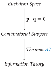
Appendix G.8 Diagrams
Figure A10.
The core Scaled Dot-Product Attention calculation.
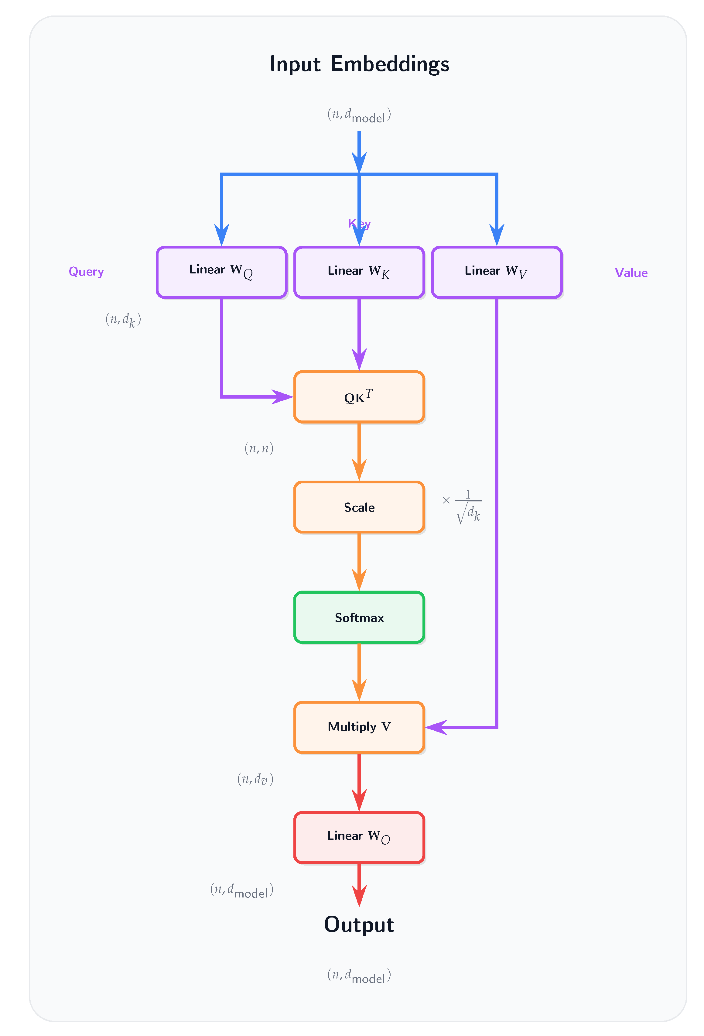
Figure A11.
The Multi-Head Attention mechanism, which runs attention in parallel.
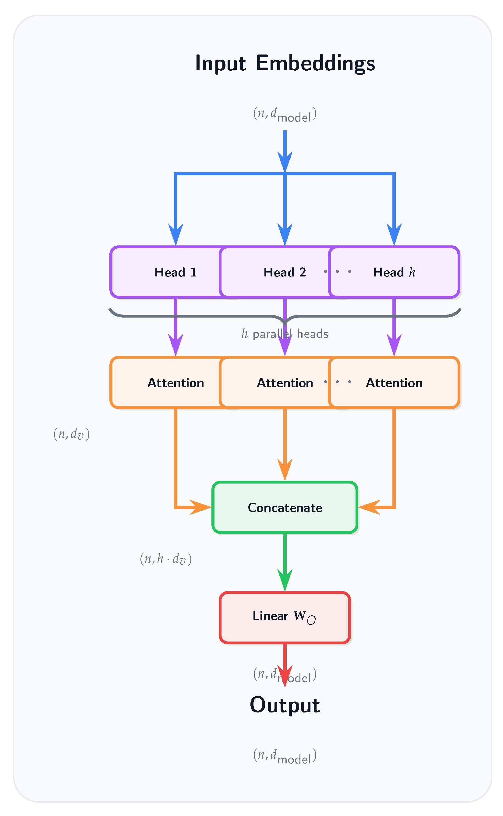
Figure A12.
The position-wise Feed-Forward Network (MLP).
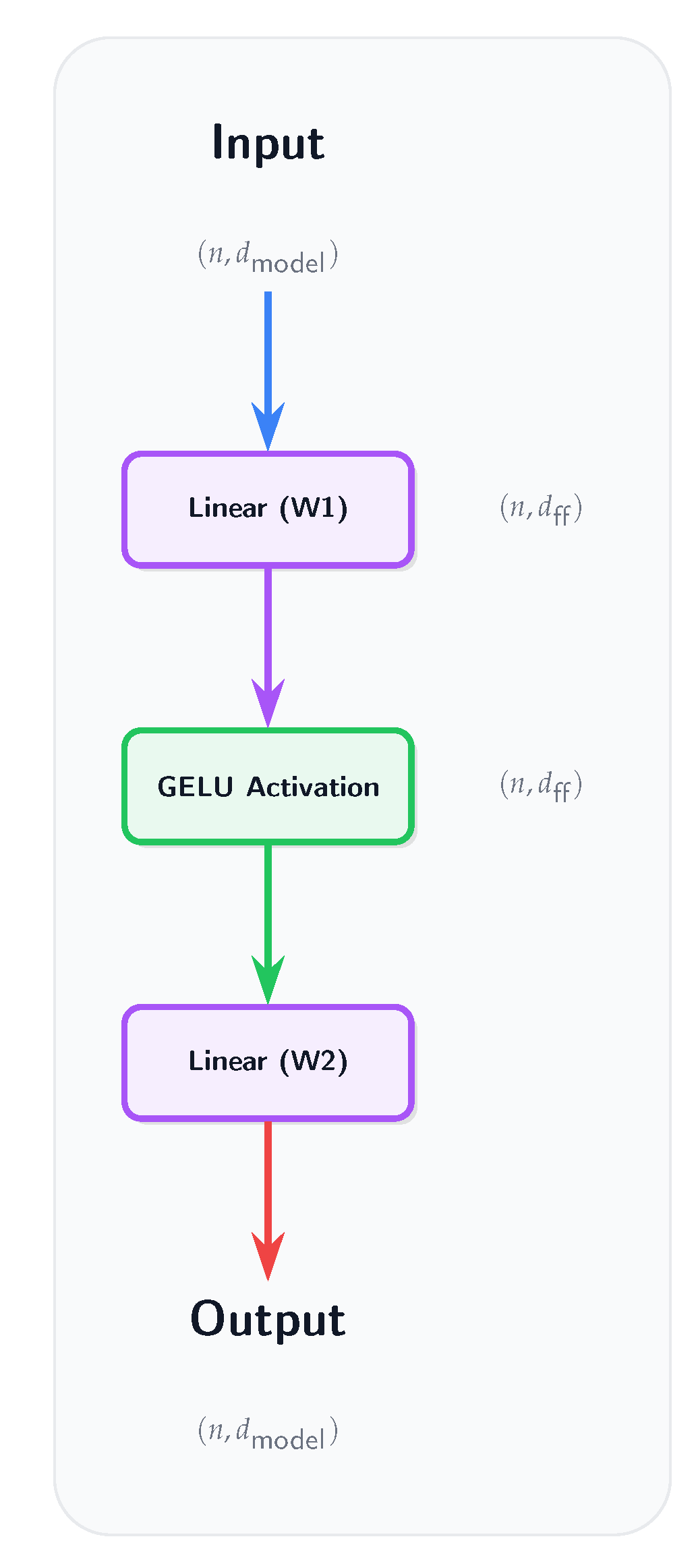
Figure A13.
The complete Encoder block, showing how Multi-Head Attention and the FFN are combined using residual connections and layer normalization.
Figure A13.
The complete Encoder block, showing how Multi-Head Attention and the FFN are combined using residual connections and layer normalization.
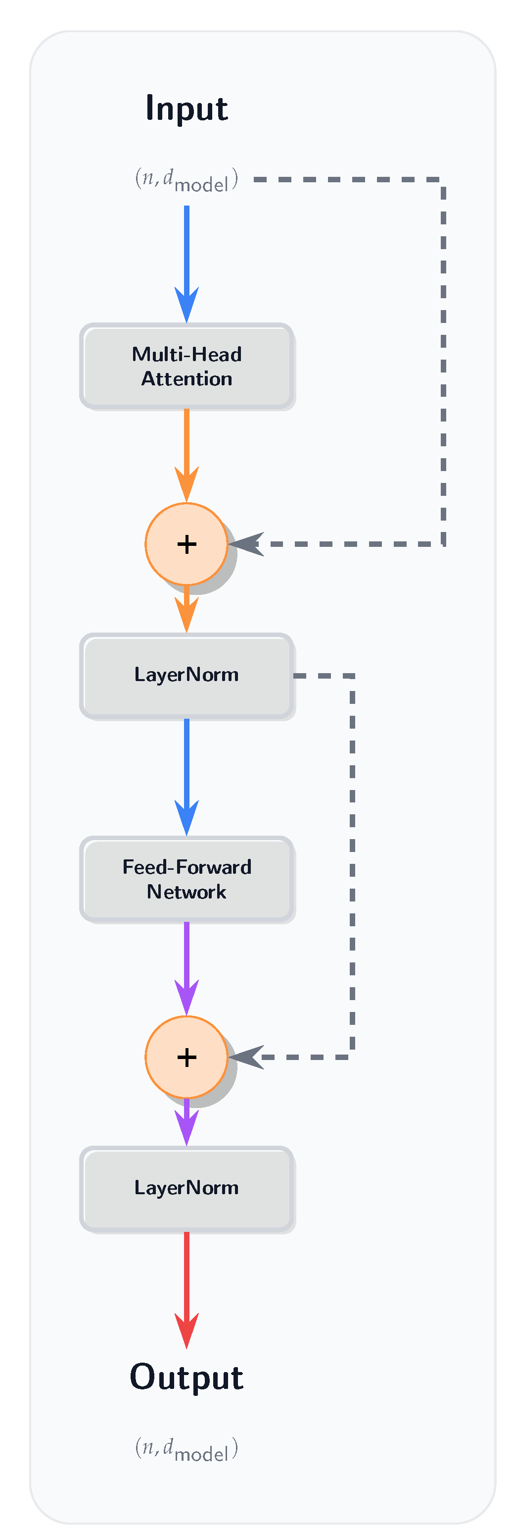
Figure A14.
A standard ResNet "Basic Block" with a residual (skip) connection. This concept of bypassing layers is a precursor to the residual connections in Transformers.
Figure A14.
A standard ResNet "Basic Block" with a residual (skip) connection. This concept of bypassing layers is a precursor to the residual connections in Transformers.
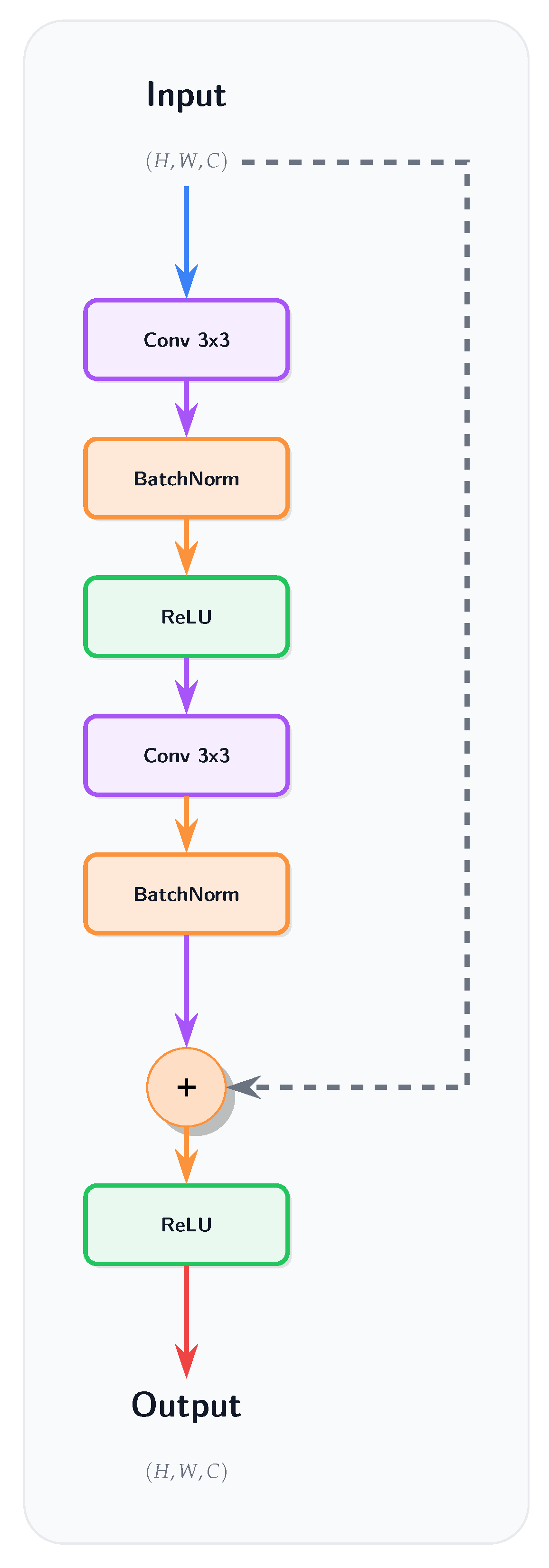
Figure A15.
A CNMN Residual Block as used in AetherResNet: a YatConv layer () followed by a linear Conv (), with no activation functions or normalization layers. The skip connection includes a projection if .
Figure A15.
A CNMN Residual Block as used in AetherResNet: a YatConv layer () followed by a linear Conv (), with no activation functions or normalization layers. The skip connection includes a projection if .
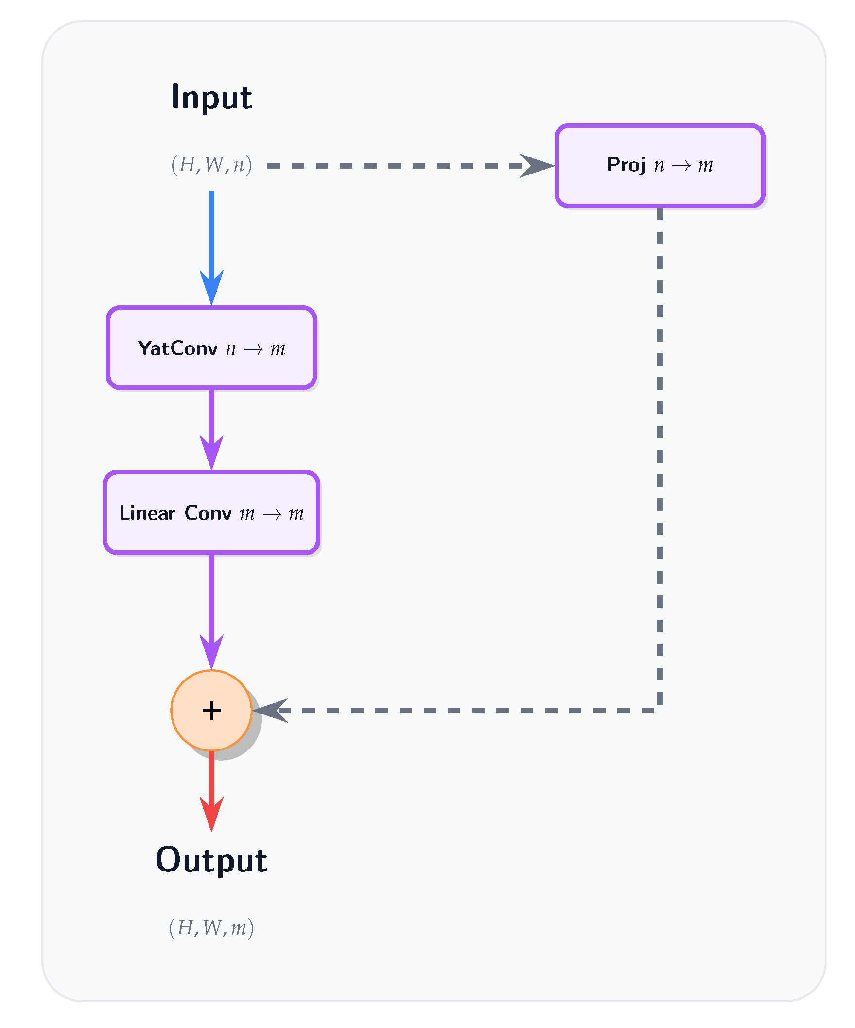
Figure A16.
A YatFormer transformer block as used in AetherGPT: Yat-Attention followed by a Yat-MLP block, each with residual connections. No projection after attention, and no normalization layers.
Figure A16.
A YatFormer transformer block as used in AetherGPT: Yat-Attention followed by a Yat-MLP block, each with residual connections. No projection after attention, and no normalization layers.
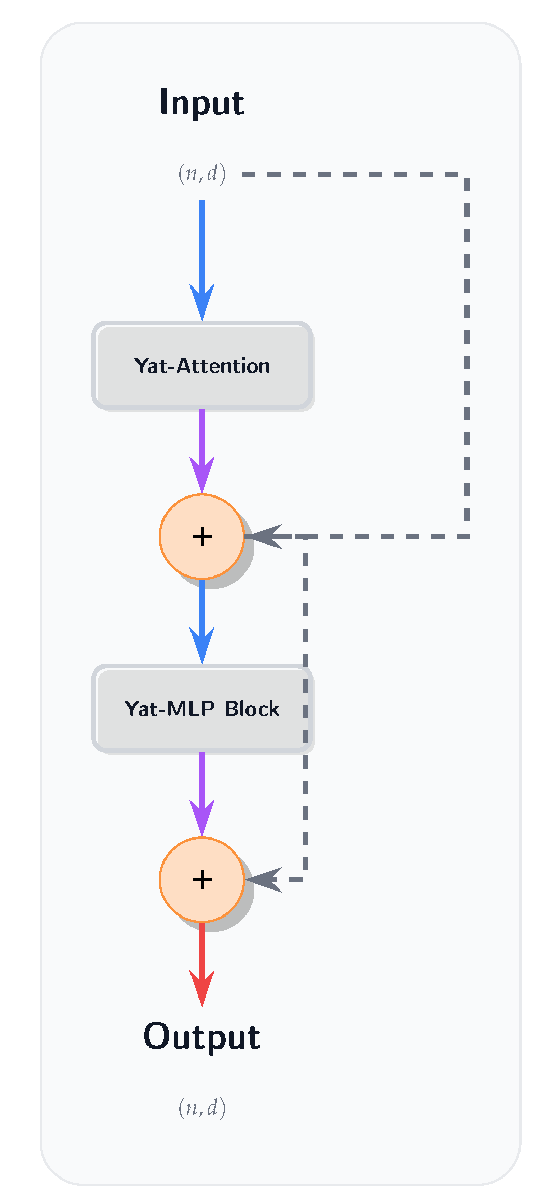
Figure A17.
The Yat-MLP block as used in AetherGPT: a YatNMN layer () followed by a linear layer (), with no expansion of the hidden dimension.
Figure A17.
The Yat-MLP block as used in AetherGPT: a YatNMN layer () followed by a linear layer (), with no expansion of the hidden dimension.
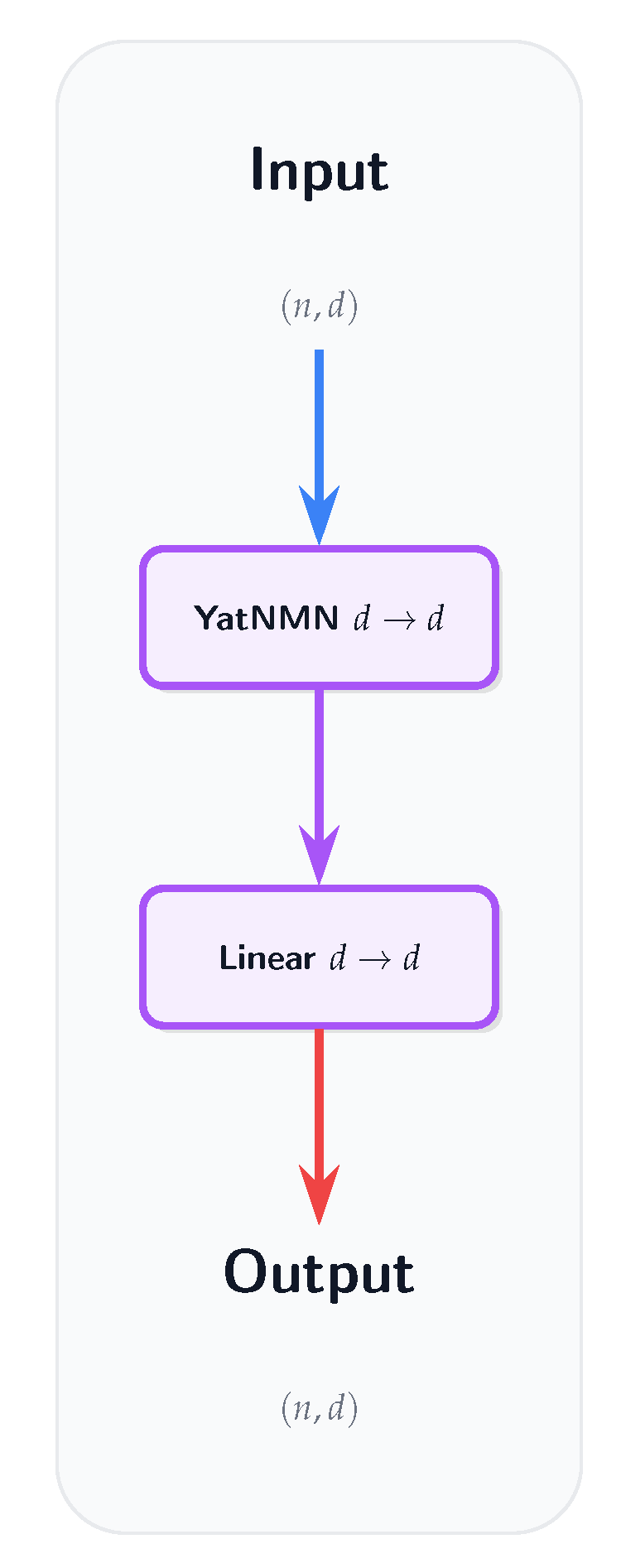
Figure A18.
The Yat-Attention block as used in AetherGPT: input embeddings are projected to queries, keys, and values; Yat-product similarity is computed between queries and keys; softermax is applied; and the output is the weighted sum of values. No projection layer after attention.
Figure A18.
The Yat-Attention block as used in AetherGPT: input embeddings are projected to queries, keys, and values; Yat-product similarity is computed between queries and keys; softermax is applied; and the output is the weighted sum of values. No projection layer after attention.
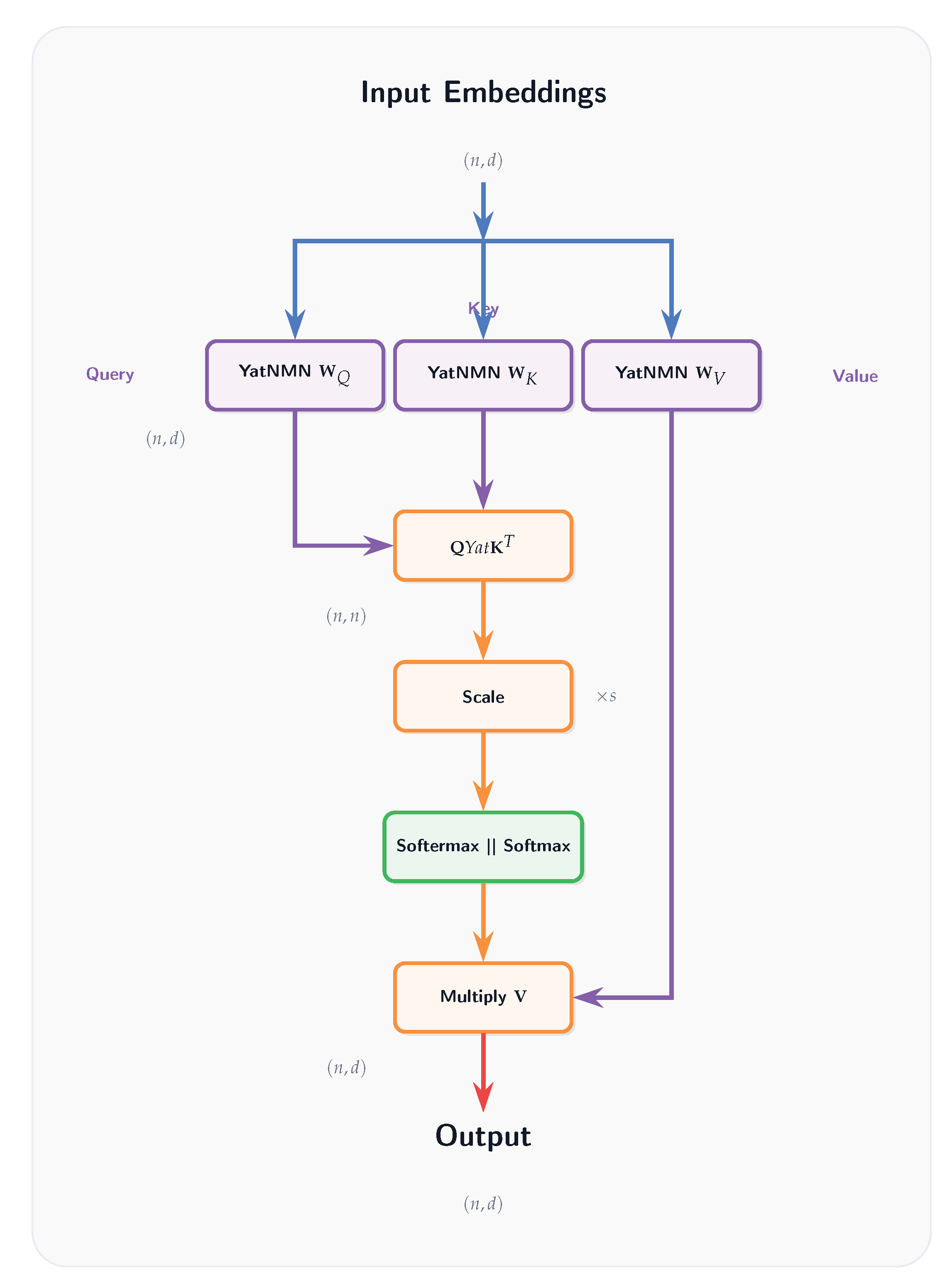
References
- Rosenblatt, F. The perceptron: a probabilistic model for information storage and organization in the brain. Psychological review 1958, 65, 386. [Google Scholar] [CrossRef]
- McCulloch, W.S.; Pitts, W. A logical calculus of the ideas immanent in nervous activity. The bulletin of mathematical biophysics 1943, 5, 115–133. [Google Scholar] [CrossRef]
- Hornik, K.; Stinchcombe, M.; White, H. Multilayer feedforward networks are universal approximators. Neural networks 1989, 2, 359–366. [Google Scholar] [CrossRef]
- Cybenko, G. Approximation by superpositions of a sigmoidal function. Mathematics of Control, Signals and Systems 1989, 2, 303–314. [Google Scholar] [CrossRef]
- Goodfellow, I.; Bengio, Y.; Courville, A. Deep learning; Vol. 1, MIT Press, 2016.
- LeCun, Y.; Bengio, Y.; Hinton, G. Deep learning. nature 2015, 521, 436–444. [Google Scholar] [CrossRef] [PubMed]
- Nair, V.; Hinton, G.E. Rectified linear units improve restricted boltzmann machines. In Proceedings of the Proceedings of the 27th international conference on machine learning (ICML-10), 2010, pp. 807–814.
- Hendrycks, D.; Gimpel, K. Gaussian Error Linear Units (GELUs), 2023, [arXiv:cs.LG/1606.08415].
- Klambauer, G.; Unterthiner, T.; Mayr, A.; Hochreiter, S. Self-normalizing neural networks. Advances in neural information processing systems 2017, 30. [Google Scholar]
- Bronstein, M.M.; Bruna, J.; LeCun, Y.; Szlam, A.; Vandergheynst, P. Geometric deep learning: going beyond euclidean data. IEEE Signal Processing Magazine 2017, 34, 18–42. [Google Scholar] [CrossRef]
- Bronstein, M.M.; Bruna, J.; Cohen, T.; Veličković, P. Geometric Deep Learning: Grids, Groups, Graphs, Geodesics, and Gauges, 2021, [arXiv:cs.LG/2104.13478].
- Balestriero, R.; Humayun, A.I.; Baraniuk, R.G. On the geometry of deep learning. NOTICES OF THE AMERICAN MATHEMATICAL SOCIETY 2025, 72. [Google Scholar] [CrossRef]
- Steck, H.; Ekanadham, C.; Kallus, N. Is cosine-similarity of embeddings really about similarity? In Proceedings of the Companion Proceedings of the ACM Web Conference 2024, 2024, pp. 887–890.
- Draganov, A.; Vadgama, S.; Bekkers, E.J. The hidden pitfalls of the cosine similarity loss. arXiv preprint 2024. arXiv:2406.16468 2024.
- Kepler, J. Ad Vitellionem paralipomena, quibus astronomiae pars optica traditur. 1604. Johannes Kepler: Gesammelte Werke, Ed. Walther von Dyck and Max Caspar, Münchenk 1939.
- Newton, I. <italic>Philosophiæ Naturalis Principia Mathematica</italic>; S. Pepys: London, 1687. Philosophiæ Naturalis Principia Mathematica; S. Pepys: London, 1687. [Google Scholar]
- de Coulomb, C.A. Premier mémoire sur l’électricité et le magnétisme. Histoire de l’Académie Royale des Sciences 1785, pp. 1–31. in French.
- Gauss, C.F. Allgemeine Lehrsätze in Beziehung auf die im verkehrten Verhältniss des Quadrats der Entfernung wirkenden Anziehungs- und Abstossungskräfte; Dietrich: Göttingen, 1835. Dietrich: Göttingen, 1835.
- Bouhsine, T. Deep Learning 2.0: Artificial Neurons That Matter – Reject Correlation, Embrace Orthogonality, 2024, [arXiv:cs.LG/2411.08085].
- Bouhsine, T.; Aaroussi, I.E.; Faysal, A.; Wang. SimO Loss: Anchor-Free Contrastive Loss for Fine-Grained Supervised Contrastive Learning. In Proceedings of the Submitted to The Thirteenth International Conference on Learning Representations, 2024. under review. 2024. under review.
- Lu, Z.; Pu, H.; Wang, F.; Hu, Z.; Wang, L. The expressive power of neural networks: A view from the width. Advances in neural information processing systems 2017, 30.
- Huang, C. ReLU networks are universal approximators via piecewise linear or constant functions. Neural Computation 2020, 32, 2249–2278. [Google Scholar] [CrossRef]
- Tanimoto, T.T. Elementary mathematical theory of classification and prediction 1958.
- Jaccard, P. Étude comparative de la distribution florale dans une portion des Alpes et des Jura. Bulletin de la Société Vaudoise des Sciences Naturelles 1901, 37, 547–579. [Google Scholar]
- Rolls, E.T.; Treves, A. The neuronal encoding of information in the brain. Progress in neurobiology 2011, 95, 448–490. [Google Scholar] [CrossRef]
- Barlow, H.B.; et al. Possible principles underlying the transformation of sensory messages. Sensory communication 1961, 1, 217–233. [Google Scholar]
- Montavon, G.; Samek, W.; Müller, K.R. Methods for interpreting and understanding deep neural networks. Digital Signal Processing 2018, 73, 1–15. [Google Scholar] [CrossRef]
- Montufar, G.F.; Pascanu, R.; Cho, K.; Bengio, Y. On the number of linear regions of deep neural networks. Advances in neural information processing systems 2014, 27. [Google Scholar]
- Ba, J.; Caruana, R. Do deep nets really need to be deep? Advances in neural information processing systems 2014, 27. [Google Scholar]
- Pezeshki, M.; Kaba, S.O.; Bengio, Y.; Courville, A.; Precup, D.; Lajoie, G. Gradient Starvation: A Learning Proclivity in Neural Networks, 2021, [arXiv:cs.LG/2011.09468].
- Wan, L.; Zeiler, M.; Zhang, S.; Le Cun, Y.; Fergus, R. Regularization of neural networks using dropconnect. In Proceedings of the International conference on machine learning. PMLR; 2013; pp. 1058–1066. [Google Scholar]
- Rumelhart, D.E.; Zipser, D. Competitive learning. Cognitive science 1985, 9, 75–112. [Google Scholar]
- Mercer, J. Functions of positive and negative type, and their connection with the theory of integral equations. Philosophical Transactions of the Royal Society of London. Series A, Containing Papers of a Mathematical or Physical Character 1909, 209, 415–446. [Google Scholar]
- Hofmann, T.; Schölkopf, B.; Smola, A.J. Kernel methods in machine learning 2008.
- Micchelli, C.A.; Xu, Y.; Zhang, H. Universal Kernels. Journal of Machine Learning Research 2006, 7. [Google Scholar]
- Schölkopf, B.; Smola, A.; Müller, K.R. Kernel principal component analysis. In Proceedings of the International conference on artificial neural networks. Springer, 1997, pp. 583–588.
- Cortes, C. Support-Vector Networks. Machine Learning 1995. [Google Scholar] [CrossRef]
- Jacot, A.; Gabriel, F.; Hongler, C. Neural tangent kernel: Convergence and generalization in neural networks. Advances in neural information processing systems 2018, 31. [Google Scholar]
- Modest, M.F. Radiative Heat Transfer, 3 ed.; Academic Press: New York, 2013. [Google Scholar]
- Knoll, G.F. Radiation Detection and Measurement, 4 ed.; John Wiley & Sons: Hoboken, NJ, 2010. [Google Scholar]
- Rea, M.S. The IESNA Lighting Handbook: Reference & Application, 9 ed.; Illuminating Engineering Society of North America: New York, 2000. [Google Scholar]
- Rappaport, T.S. Wireless Communications: Principles and Practice, 2 ed.; Prentice Hall: Upper Saddle River, NJ, 2002. [Google Scholar]
- Skolnik, M.I. Radar Handbook, 3 ed.; McGraw-Hill Education: New York, 2008. [Google Scholar]
- Aki, K.; Richards, P.G. Quantitative Seismology, 2 ed.; University Science Books: Sausalito, CA, 2002. [Google Scholar]
- Batchelor, G.K. An Introduction to Fluid Dynamics; Cambridge University Press: Cambridge, UK, 2000. [Google Scholar]
- Anderson, J.E. The Gravity Model. Annual Review of Economics 2011, 3, 133–160. [Google Scholar] [CrossRef]
- Schölkopf, B.; Smola, A.; Müller, K.R. Nonlinear component analysis as a kernel eigenvalue problem. Neural computation 1998, 10, 1299–1319. [Google Scholar] [CrossRef]
- Williams, C.K.; Rasmussen, C.E. Gaussian processes for machine learning; Vol. 2, MIT press Cambridge, MA, 2006.
- Ng, A.; Jordan, M.; Weiss, Y. On spectral clustering: Analysis and an algorithm. Advances in neural information processing systems 2001, 14. [Google Scholar]
- Schölkopf, B.; Platt, J.C.; Shawe-Taylor, J.; Smola, A.J.; Williamson, R.C. Estimating the support of a high-dimensional distribution. Neural computation 2001, 13, 1443–1471. [Google Scholar] [CrossRef]
- Williams, C.; Seeger, M. Using the Nyström method to speed up kernel machines. Advances in neural information processing systems 2000, 13. [Google Scholar]
- Rahimi, A.; Recht, B. Random features for large-scale kernel machines. Advances in neural information processing systems 2007, 20. [Google Scholar]
- Boser, B.E.; Guyon, I.M.; Vapnik, V.N. A training algorithm for optimal margin classifiers. In Proceedings of the Proceedings of the Fifth Annual Workshop on Computational Learning Theory, New York, NY, USA, 1992; COLT ’92, p. 144–152. [CrossRef]
- Lecun, Y.; Bottou, L.; Bengio, Y.; Haffner, P. Gradient-based learning applied to document recognition. Proceedings of the IEEE 1998, 86, 2278–2324. [Google Scholar] [CrossRef]
- Vaswani, A.; Shazeer, N.; Parmar, N.; Uszkoreit, J.; Jones, L.; Gomez, A.N.; Kaiser, .; Polosukhin, I. Attention is all you need. Advances in neural information processing systems 2017, 30. 2017, 30.
- Dosovitskiy, A.; Beyer, L.; Kolesnikov, A.; Weissenborn, D.; Zhai, X.; Unterthiner, T.; Dehghani, M.; Minderer, M.; Heigold, G.; Gelly, S.; et al. An Image is Worth 16x16 Words: Transformers for Image Recognition at Scale, 2021, [arXiv:cs.CV/2010.11929].
- Tolstikhin, I.; Houlsby, N.; Kolesnikov, A.; Beyer, L.; Zhai, X.; Unterthiner, T.; Yung, J.; Steiner, A.; Keysers, D.; Uszkoreit, J.; et al. MLP-Mixer: An all-MLP Architecture for Vision, 2021. arXiv:2105.01601 [cs].
- Liu, H.; Dai, Z.; So, D.R.; Le, Q.V. Pay Attention to MLPs, 2021. arXiv:2105.08050 [cs].
- Ivakhnenko, A.G. Polynomial theory of complex systems. IEEE transactions on Systems, Man, and Cybernetics 1971, pp. 364–378.
- Livni, R.; Shalev-Shwartz, S.; Shamir, O. An Algorithm for Training Polynomial Networks, 2014, [arXiv:cs.LG/1304.7045].
- Lee-Thorp, J.; Ainslie, J.; Eckstein, I.; Ontanon, S. FNet: Mixing Tokens with Fourier Transforms, 2022. arXiv:2105.03824 [cs].
- Horn, R.A.; Johnson, C.R. Matrix Analysis; Cambridge University Press, 2012.
- Cover, T.M.; Thomas, J.A. Elements of Information Theory; Wiley-Interscience, 2006.
- Schölkopf, B.; Smola, A.J. Learning with Kernels: Support Vector Machines, Regularization, Optimization, and Beyond; MIT Press, 2002.
- Rudin, W. Functional Analysis; McGraw-Hill, 1991.
- Hornik, K. Approximation capabilities of multilayer feedforward networks. Neural Networks 1991, 4, 251–257. [Google Scholar] [CrossRef]
- Rudin, W. Real and Complex Analysis; McGraw-Hill, 1987.
Figure 2.
Visualization of the Yat-product’s vector field in 2D and 3D spaces. The heatmaps illustrate how the Yat-product, unlike traditional similarity measures, creates a potential well around the weight vector , reflecting both alignment and proximity. This figure embodies the paper’s philosophy of unifying geometric alignment and spatial closeness within a single neural operator, inspired by physical interaction fields. The resulting landscape demonstrates how the Yat-product enables neural units to act as localized fields of influence, supporting our approach to interpretable, geometry-aware neural computation.
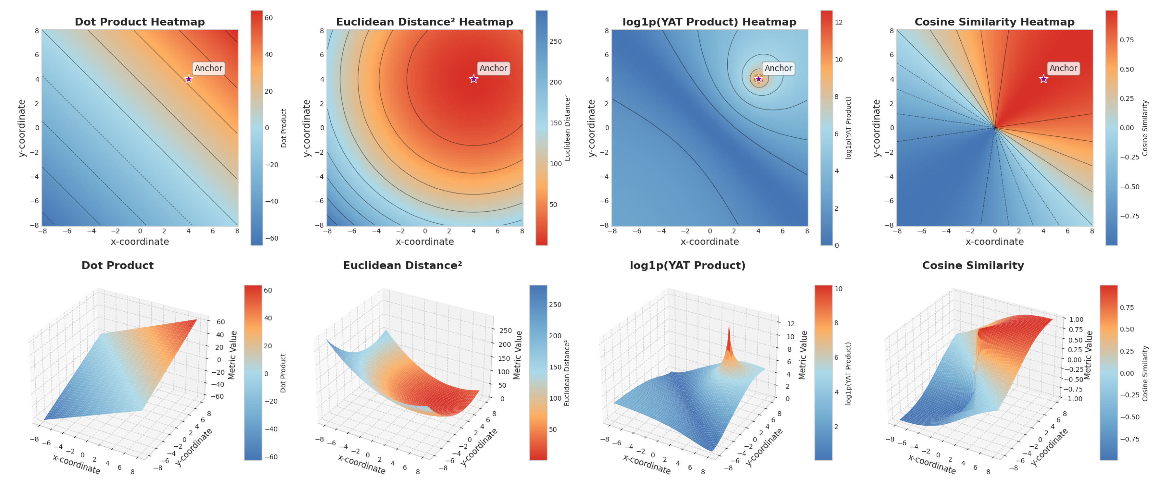
Figure 3.
Comparison of the Yat-product with other metrics (dot product, cosine similarity, and Euclidean distance) in three distinct settings: (a) scaling vectors linearly by a factor s, (b) rotating the anchor vector, and (c) varying the distance of vectors around the anchor. The Yat-product’s unique sensitivity to both alignment and proximity is highlighted across these scenarios.
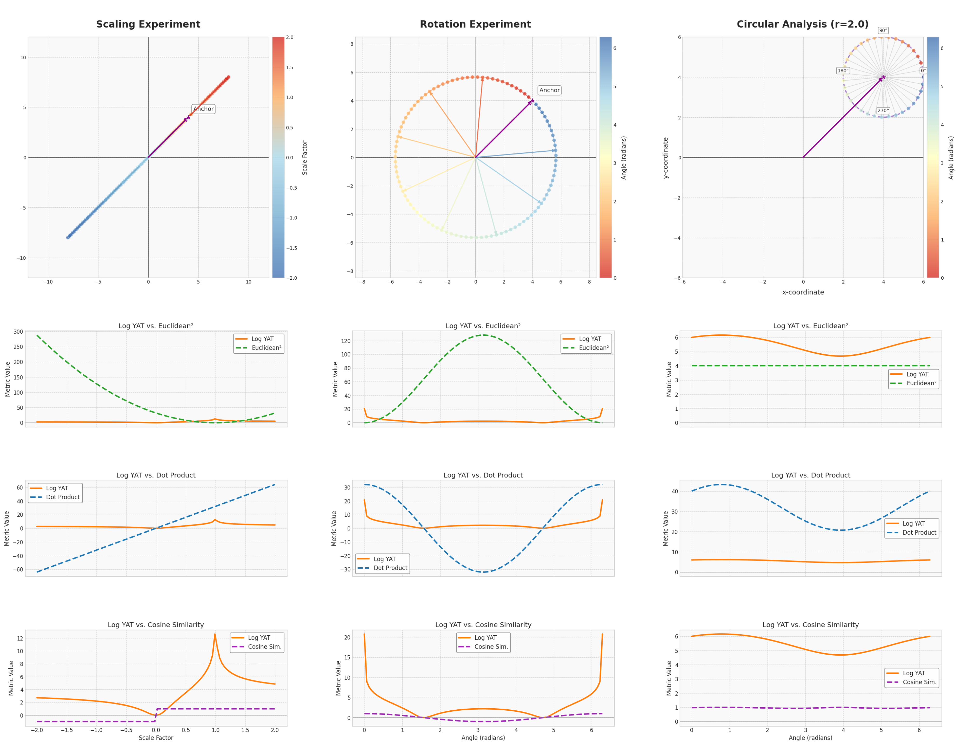
Table 2.
Final validation loss comparison between GPT2 and Aether-GPT2 on 600m tokens of Fineweb.
| Dataset | GPT2 | Aether-GPT2 |
|---|---|---|
| Fineweb | 2.69 | 2.83 |
Disclaimer/Publisher’s Note: The statements, opinions and data contained in all publications are solely those of the individual author(s) and contributor(s) and not of MDPI and/or the editor(s). MDPI and/or the editor(s) disclaim responsibility for any injury to people or property resulting from any ideas, methods, instructions or products referred to in the content. |
© 2025 by the authors. Licensee MDPI, Basel, Switzerland. This article is an open access article distributed under the terms and conditions of the Creative Commons Attribution (CC BY) license (http://creativecommons.org/licenses/by/4.0/).
Copyright: This open access article is published under a Creative Commons CC BY 4.0 license, which permit the free download, distribution, and reuse, provided that the author and preprint are cited in any reuse.


