
Submitted:
20 June 2025
Posted:
24 June 2025
You are already at the latest version
Abstract
This paper proposes advanced soft sensor models based on machine learning and deep learning for real-time estimation of top and bottom product compositions in a Heat-Integrated Distillation Column (HIDiC). Conventional composition analyzers, such as gas chromatographs, are expensive and suffer from significant measurement delays, making them less efficient for real-time measurement and control. As a cost-effective alternative, soft sensors can be developed using process data from a high-fidelity dynamic HIDiC simulation, with tray temperatures as the model inputs. This research develops and evaluates both linear and nonlinear modeling strategies for composition estimation in a HIDiC, including Principal Component Regression (PCR), Artificial Neural Network (ANN), and marking the first application of its kind in HIDiC modeling a Bidirectional Long Short-Term Memory (BiLSTM) network. While PCR and ANN achieved reasonable accuracy, their performance was limited by an inability to fully capture the temporal dependencies and complex nonlinearities inherent in the distillation process. In contrast, the BiLSTM model, leveraging its deep learning architecture and temporal memory capabilities, successfully learned long-range dependencies and intricate dynamic patterns in the process data. Comprehensive performance evaluation based on Mean Absolute Error (MAE), Mean Squared Error (MSE), and the coefficient of determination (R²) demonstrated that the BiLSTM model outperformed the traditional models significantly. The results confirm that the BiLSTM-based soft sensor not only enhances prediction accuracy but also represents a novel and effective approach for real-time composition estimation in HIDiC systems, offering great potential for advanced monitoring and control applications.
Keywords:
distillation column
; heat integration
; heat integrated distillation column
; bidirectional long short-term memory
; artificial neural network
; principal component regression
; soft sensor
1. Introduction
Heat-Integrated Distillation Columns (HIDiCs) represent a cutting-edge advancement in distillation technology, designed to enhance energy efficiency through internal heat integration. Unlike conventional distillation systems, HIDiCs facilitate direct heat transfer between the rectifier and stripper sections by exploiting boiling point differences, thereby improving separation efficiency and reducing energy demand [1]. Figure 1 illustrates the block diagram of the process, highlighting the heat transfer between the two sections.
Numerous control strategies have been proposed to manage the inherent complexity and strong interactions within HIDiCs. Bisgaard et al. [2] conducted a systematic analysis to identify appropriate manipulated and controlled variables through degrees of freedom analysis, operational mapping, and constraint identification. Their dual-layer strategy, combining regulatory and supervisory control, showed effective performance in dynamic simulations. For the control of a high-purity heat integrated distillation column, an adaptively corrected set-point sensitive stage temperature control technique is suggested in [3]. First, the temperature profile movement situation, which primarily includes the functions of the temperature profile and its moving velocity, is established to characterize the dynamics of the system to ensure the logic of the set-point correction. The temperature profile function conveys the shape of the stage's temperature distribution, and the temperature profile's moving velocity indicates changes in the position of the profile. The temperature measurement locations are then chosen using a modified version of the PCA approach, and the profile function's profile parameters are computed using the chosen observations. In [4], diverse heat-integrated pressure swing distillation processes, such as conventional and entrainer-assisted pressure swing distillation, partially and fully heat-integrated pressure swing distillation all employ differential temperature control to regulate the sensitive-stage temperature under operation pressure fluctuations of the high-pressure column. Under operation pressure variations, the differential temperature control modifies slightly, producing useful outcomes. The computation of Integral Absolute Error of product purities confirms that the dynamic performances of differential temperature control and pressure-compensated temperature control for each process are nearly identical.
In [5], the mixture was separated through the pervaporation process, and all reactive distillation and pervaporation-related parameters—such as permeate stream pressure, the number of modules, and the temperature of the inflow to each module—were considered as optimization variables. All variables were simultaneously optimized, with total annual cost used as the objective function. In addition, the GA and PSO algorithms were integrated to optimize the process. The number of heat exchangers between the two rectifying and stripping sections was determined using the optimization algorithm, and the internally heat-integrated distillation column (HIDiC) approach was employed to reduce energy costs in the reactive distillation column. The nonlinear modelling of HIDiC is quite complex, and first-principles approaches struggle to manage the nonlinearities due to limitations in model accuracy and parameter reliability. In [6], the relative stability of the profile pattern in distillation columns is investigated. The function structure of the profile pattern remains unchanged, and the system dynamics are reflected in the temporal variations of its parameters. A nonlinear modelling approach is developed based on this stable profile pattern. Two basic methods for updating the profile parameters are proposed using different inflexion point calculation techniques. Subsequently, dynamic connections between sensitive and top/bottom stages are established based on the update methods. These methods are integrated into control loops, resulting in two fundamental control strategies. A simulation study compares HIDiC with conventional distillation, applying various inflexion point velocity estimation techniques to suit the specific characteristics of each process. The results show that the proposed strategies significantly reduce product purity offsets compared to PID control. The comparative analysis of the control schemes further highlights their strengths, weaknesses, and selection criteria.
To identify and control the HIDiC system, a novel non-parametric support vector regression (SVR) approach is proposed in [7]. The support vector regression parameters were optimized using the artificial bee colony (ABC) algorithm, which outperformed other meta-heuristic algorithms. In terms of root mean square error and coefficient of determination, the SVR model delivered superior performance compared to artificial neural network-based methods.
A hybrid approach combining Mixed-Integer Linear Programming (MILP) with Simulated Annealing achieved 71.9% energy savings and 15.9% cost reduction with fewer iterations [8].
Stochastic optimization integrated with mechanical vapor recompression resulted in a 29.55% reduction in total annual cost (TAC), 55.99% lower energy consumption, and significant CO₂ emission cuts [9]. Another stochastic method, combined with Aspen Plus, handled close-boiling mixtures effectively despite high computational demands [10]. The Binary Update Multi-Decision Algorithm (BUMDA) outperformed traditional approaches in heat duty reduction (5–20%) and computational speed [11]. Furthermore, a reactive extractive distillation system optimized with Particle Swarm Optimization (PSO) achieved a 56.5% CO₂ emission reduction and increased energy efficiency from 38.27% to 43.10% [12]. Other notable innovations include: A three-side stream extractive configuration with intermediate reboilers, which cut TAC by 29.02% and enhanced thermodynamic performance, albeit at the cost of increased control complexity [13]. A novel desalination system combining membrane distillation and dehumidification, achieving 51.2% energy and 35.3% cost savings [14]. An optimization framework integrating tray hydraulics to improve convergence and industrial applicability for complex columns [15]. A heterogeneous azeotropic distillation process using heat pumps, which lowered energy use and emissions despite higher capital costs [16]. A dividing wall column design for methyl methacrylate that minimized TAC and offered a short payback period despite elevated energy needs [17]. A hybrid configuration for xylene isomer separation integrating extractive distillation, vapor recompression, and feed preheating resulting in 14.2% TAC and 30.2% CO₂ reductions [18].
In terms of modelling, Wave Propagation Models (WPMs) offer a streamlined and transparent approach by avoiding complex numerical discretization such as collocation methods. However, traditional WPMs depend on strong assumptions (e.g., ideal mixtures, constant holdup), limiting their applicability to dynamic or non-ideal systems. To overcome these limitations, Schulze et al. [19] extended Kienle’s WPM using global hydraulic correlations and nonlinear wave theory to develop the Transient Wave Propagation Model (TWPM). While early WPM applications focused on binary systems, recent studies have expanded their use to multi-component, multi-section, and dynamic column operations. For example, Han et al. [20] demonstrated the robustness of WPM in controlling the semi-continuous startup of a two-column configuration. Despite these advancements, the inherent nonlinearity and high dimensionality of HIDiC systems continue to pose significant optimization challenges. Conventional methods often fall short in large-scale scenarios due to the combinatorial explosion of variables and constraints. In response, hybrid optimization algorithms particularly those tailored for solving Mixed-Integer Nonlinear Programming (MINLP) problems have emerged as powerful tools. These approaches leverage the complementary strengths of multiple algorithms to address the complex trade-offs in HIDiC design and operation [21,22,23].
In distillation processes, accurate and timely measurement of top and bottom product compositions is essential for effective closed-loop control. However, direct online composition measurements typically obtained via gas chromatographs are often constrained by high costs, slow sampling rates, and time delays caused by sampling and analysis procedures. These limitations hinder real-time feedback, leading to control delays, reduced product quality, and inefficient energy use. To overcome these challenges, soft sensors are widely employed to estimate product compositions using easily measurable process variables such as tray temperatures. This study presents the first application of BiLSTM networks for soft sensing of top and bottom product compositions in a HIDiC. The proposed BiLSTM-based model captures the system’s nonlinear and dynamic behavior with high accuracy, enabling real-time composition estimation in a highly complex and thermally coupled distillation process. To demonstrate the effectiveness of the proposed approach, BiLSTM performance is systematically compared with traditional models, including PCR and ANN. This comparison highlights BiLSTM’s superior capability in capturing the nonlinear dynamics of the HIDiC system and delivering more accurate and reliable real-time composition estimates. This marks a significant step in data-driven inferential control of HIDiCs, showcasing the potential of advanced models for handling process complexity and nonlinearity.
2. System Description
The mechanistic nonlinear model of the HIDiC used in this study is adopted from [24]. The column consists of 54 trays, following the assumptions of negligible vapor holdup, constant liquid holdup, perfect mixing of liquid and vapor on each tray, instantaneous heat transfer between the rectifying and stripping sections, negligible pressure drop in both sections, and constant latent heat and relative volatility. The nominal operating conditions used in this study are summarized in Table I, with a reference setpoint of 99.5% for the top composition (benzene) and 0.5% for the bottom composition (toluene) as in [25,26].

Table 1.
Steady state operating conditions of the HIDiC.
| Items | Values |
|---|---|
| Number of stages | 52 |
| Compression to ratio | 2.55 |
| Pressure of feed | 1.013 kPa |
| Pressure decreases across trays | 0.0035 kPa |
| Each stage's heat exchange area | 5 m2 |
| Rate of feed | 83.3 mol s-1 |
| Flow rate of reflux | 56.2 mol s-1 |
| Condenser duty | 853 kW |
| Compressor duty | 483 kW |
| Reboiler duty | 791 kW |
| Feed-in pre-heater duty | 500 kW |
| Time constant for compressor | 10 s |
| Condenser and reboiler time constants less than | 300 s |
| Weir height of less than | 0.1 meters |
| Elevation above the weir | <1.25% |
| The compressor's isentropic efficiency | 72% |
| Feed composition: (benzene/toluene) | 0.5 / 0.5 mol% |
| Coefficient of Heat Transfer Overall | 0.6 kW K-1 m-2 |
3. Machine Learning Models
In modern process industries, accurate real-time estimation of key process variables such as product compositions is vital for effective control and optimization. Traditional analytical instruments like gas chromatographs are often limited by high latency, delay and maintenance demands. To overcome these limitations, machine learning (ML) offers a robust data-driven approach for soft sensor development, enabling the indirect estimation of hard-to-measure variables using readily available process data. This section outlines the architecture and implementation of ML-based soft sensor models for estimating the top and bottom compositions in a HIDiC. To ensure realistic and robust training, the dataset underwent the following preprocessing steps: Measurement Noise Simulation: Gaussian white noise (mean = 0, standard deviation = 0.03%) was added to the simulated composition data to mimic physical sensors where measurement noises always exist. Standardization: All input variables and target outputs were standardized using their respective means and standard deviations, improving model convergence and ensuring uniform feature scaling.
To analyses the sensor development, PCR, ANN, and BiLSTM-based sensors were developed and evaluated. To ensure a fair and consistent comparison, all three models were trained and tested using the same dataset, with tray temperature profiles as input features and the corresponding product compositions as target outputs. Figure 2 shows the block diagram of the sensor development process using the tray temperature data. The dataset consisted of 3000 samples, each representing a snapshot of tray temperature profiles paired with corresponding product composition measurements. For model development, the data were split into 80% for training (2400 samples) and 20% for testing (600 samples), ensuring that all models PCR, ANN, and BiLSTM were trained and validated on the same partitions to maintain consistency in performance evaluation.
The inputs to the PCR model consisted of 54 tray temperatures collected from dynamic simulations of the HIDiC system. These inputs were standardized using z-score normalization. Principal Component Analysis (PCA) was applied to reduce the dimensionality of the input data before regression. Instead of selecting the number of principal components based solely on a retained variance threshold (e.g., ≥99%), which may not yield optimal predictive performance, cross-validation was employed to determine the number of components that minimized the prediction error in the PCR model. Based on the 5-fold cross-validation results using MSE as the performance metric, the optimal number of principal components (PCs) was determined to be 28 for the top composition and 26 for the bottom composition. These values correspond to the lowest testing MSE observed across the cross-validation folds, indicating that they offer the best generalization performance for their respective PCR models.
A linear regression model was then fitted to the principal components to estimate the top and bottom compositions.
3.1. Artificial Neural Network
To model the nonlinear relationship between tray temperatures and product compositions in the HIDiC, a feedforward ANN was developed using supervised learning, as illustrated in Figure 3. The input features—standardized tray temperature profiles—were mapped to the corresponding top and bottom compositions. All inputs and targets were normalized to have zero mean and unit variance. The ANN architecture consists of two hidden layers with 20 and 10 neurons, respectively. The network structure was selected based on empirical testing, where multiple configurations were evaluated for their prediction accuracy and generalization performance on a validation dataset. A moderately sized architecture was chosen to balance model complexity and the risk of overfitting. In terms of activation functions, the tangent sigmoid (tansig) function was used in the first hidden layer to model the input nonlinearity, while the logarithmic sigmoid (logsig) was employed in the second hidden layer to enhance nonlinear representation. The output layer utilized a linear (purelin) activation function, which is appropriate for continuous regression tasks such as composition estimation.
To further improve generalization and mitigate overfitting, Bayesian Regularization (trainbr) was selected as the training algorithm. This method automatically penalizes overly complex models by adjusting the effective number of parameters during training. The training was configured for up to 1000 epochs, with a minimum gradient threshold of 1e-7, and incorporated an early stopping criterion triggered after 10 consecutive validation failures (max_fail = 10). A small regularization parameter (0.01) was also applied to encourage smoother model outputs. To ensure reproducibility, the network was initialized with fixed random seeds, and training was carried out using MATLAB’s train function. This carefully tuned configuration demonstrated robust predictive performance, as detailed in the results section.
3.2. Bidirectional Long Short-Term Memory
To enhance the learning of temporal patterns in tray temperature data, a BiLSTM network was employed to estimate the top and bottom compositions in the HIDiC. Unlike standard LSTM, the BiLSTM processes input sequences in both forward and backward directions, simultaneously capturing past and future context. This bidirectional learning capability enhances prediction accuracy, especially under dynamic and transient conditions. Figure 4 showed the architecture of the BiLSTM. Standardized temperature sequences were used as inputs, and the model was trained using a sequence-to-one mapping strategy for real-time soft sensing applications. The BiLSTM network architecture was designed to learn the nonlinear and temporal dependencies between tray temperature profiles and product compositions in the HIDiC system. The input data were structured as sequences of length 10, selected through empirical evaluation to provide sufficient historical context for accurate prediction while maintaining computational tractability. Each input sequence captured 10 consecutive time steps of 54 standardized tray temperatures, and the corresponding target was the standardized composition at the subsequent time step.
The BiLSTM layer was configured with 100 hidden units, a value chosen based on iterative experimentation with different network sizes. Various configurations were evaluated by training on the dataset and monitoring their prediction performance and convergence behaviour. The selected number of units offered a good trade-off between model capacity and training stability. The output from the BiLSTM layer was passed through a fully connected layer and a regression output layer, optimized using mean squared error (MSE) loss. Training was carried out using the Adam optimizer with a learning rate of 0.005, a maximum of 200 epochs, and a gradient threshold of 1, which were determined through manual tuning to achieve reliable convergence without overfitting. This architecture and training setup were found to consistently produce accurate and robust predictions for product composition, as confirmed by the results presented in the evaluation section.
4. Results and Discussion
This section presents the results and analyzes the performance of PCR, ANN, and BiLSTM data-driven models developed to estimate the top and bottom product compositions in HIDiC. The dataset 3,000 samples of tray temperature were used, the data were split into 80% for training (2400 samples) and 20% for testing (600 samples), Standard metrics such as the MAE, MSE, and R² were used to evaluate the performance of the models.
Figure 5 and 6 shows the performance of the PCR model in predicting the top and bottom product composition. The upper subplot illustrates a close agreement between the actual compositions values and those predicted by the PCR model across the entire simulation time. The predicted trajectory successfully tracks the major dynamic trends and steady-state regions, including sharp drops and gradual recoveries, indicating the model’s effectiveness in capturing the underlying system behavior.
However, as shown in the lower subplot of Figures, the prediction error fluctuates over time, particularly in dynamic transition regions around 400–1000 and 1800–2500 minutes, where rapid changes in composition occur. The error mostly remains within ±0.5%, which is reasonably acceptable for many control applications, considering that PCR is a linear method based on a reduced set of principal components. The slight increase in prediction error during highly dynamic intervals can be attributed to PCR’s inherent limitations in modeling nonlinear relationships and temporal dependencies within time-series data. PCR relies on the projection of high-dimensional input features tray temperatures into a lower-dimensional space, which may discard some nonlinear dynamics crucial for precise tracking.
Figure 7 and Figure 8 show the performance of the ANN model in predicting the top and bottom product compositions of the HIDiC. The upper subplots illustrate an excellent match between the actual top and bottom compositions values and the predicted ANN model over the simulation period. The predicted trajectory aligns closely with the true values across both steady-state regions and periods of dynamic change, demonstrating the ANN’s capability to learn and represent complex nonlinear relationships in the process data. The lower subplot in Figure 7 and Figure 8 presents the prediction errors over time. The error remains tightly bounded, typically within ±0.3%, which confirms the model's robustness and suitability for real-time estimation tasks. Compared to PCR, the ANN model maintains more consistent accuracy, even in dynamic regions of the process such as between 400–1000 minutes and 1800–2500 minutes where composition changes rapidly due to operational transitions.
The ANN’s superior performance highlights its strength in capturing nonlinear and multivariate dependencies among input variables, such as tray temperatures and other process measurements. Unlike PCR, which reduces dimensionality at the expense of potentially discarding important dynamic features, the ANN uses fully connected layers and nonlinear activation functions to retain and learn complex mappings from input to output.
Figure 9 and Figure 10 illustrates the performance of the BiLSTM network in predicting the top and bottom product composition of the HIDiC. In the upper subplots, the predicted values closely follow the actual bottom composition over the entire simulation period. The BiLSTM model accurately captures the dynamic trends, including rapid increases, plateaus, and sharp declines, highlighting its strength in modeling complex time-dependent behaviors. The lower subplots in figures show the prediction error across the simulation time. The error remains well within ±0.1% for most of the simulation, with minimal spikes even during periods of sudden changes in composition. This tight error distribution indicates a significant enhancement in prediction precision compared to both PCR and ANN models. Due to the use of sequence-based learning, predictions begin only after the initial window length (10 samples), which shifts the alignment of actual and predicted signals. This design ensures the model captures temporal context but results in plots that do not start from the very first time point. Nonetheless, the prediction accuracy stabilizes quickly after this initial offset. Rolling average plots for both training and testing predictions indicate the model performs with low bias and moderate noise, especially in high-variation regions of the dataset. This is consistent with the high R² value (0.9991), confirming the model's ability to explain most of the variance in the output.
The superior performance of the BiLSTM model can be attributed to its inherent ability to capture long-range temporal dependencies by processing input sequences in both forward and backward directions. Unlike traditional ANN models, which lack memory of previous time steps, BiLSTM networks are well-suited for sequence prediction tasks in this dynamic process where current states are influenced by past trends and inputs.
To assess the effectiveness of the proposed BiLSTM model, its performance is further compared against ANN and PCR via the MAE, MSE, and R². Table 2 summarizes the comparative results for both top and bottom product compositions computed on training and testing datasets. For the top composition, while all models performed well, the BiLSTM model achieved the highest R² of 0.9980, indicating a better fit to the actual top composition than both PCR and ANN. The BiLSTM model’s superior R² suggests it captured the system’s underlying nonlinear dynamics more comprehensively. The PCR model, while significantly simpler and faster to train, underperformed due to its inherent linearity and lack of temporal modelling capability. This confirms that deep learning models, especially BiLSTM, are more appropriate for time-dependent chemical process variables like column compositions.
For the bottom composition, the BiLSTM again outperformed the other models, achieving the highest R² of 0.9991. The ANN model came close in performance, but BiLSTM offered better generalization and temporal tracking, as seen in the prediction plots and residual errors. PCR's performance on the bottom composition was relatively acceptable but again limited by its linear assumptions and static nature, which restrict its ability to adapt to process dynamics. PCR is efficient for quick deployment and interpretable modelling but lacks the ability to handle nonlinear and dynamic behaviour. ANN offers better nonlinear modelling than PCR but lacks memory and struggles with time-sequenced data unless explicitly structured with delays. BiLSTM provides the most accurate and consistent predictions due to its bidirectional memory mechanism, which captures both forward and backward dependencies in process variables. These results strongly justify the use of BiLSTM networks as the preferred soft sensor architecture for real-time monitoring and control in HIDiC systems.
Figure 11.
Bar chat Comparative performances of three soft sensor models.
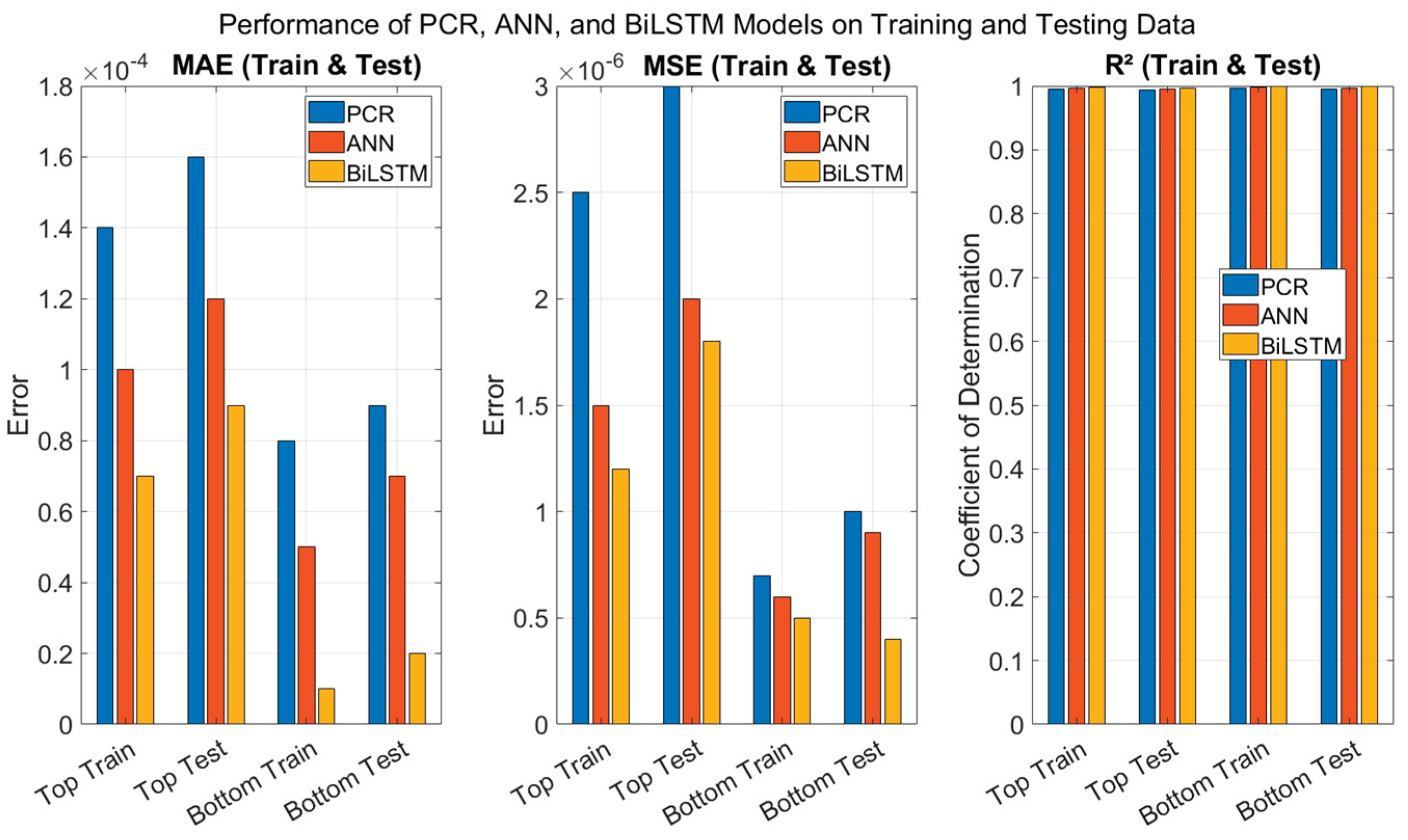
Across all the evaluation metrics, the BiLSTM model consistently outperforms ANN and PCR, confirming its ability to model complex and dynamic relationships in the data as showed in figure 11. For the training set, BiLSTM achieves the lowest MAE values of 0.00007 (top) and 0.00001 (bottom), and the lowest MSE values of 1.2×10⁻⁶ and 5.0×10⁻⁷, respectively. In terms of R², BiLSTM records 0.9980 (top) and 0.9991 (bottom), indicating a very good fit. On the testing set, BiLSTM maintains its superior performance, with MAEs of 0.00009 (top) and 0.00002 (bottom), and R² values of 0.9972 and 0.9987, respectively. This strong generalization capability is critical for real-time control applications. The ANN model performs slightly below BiLSTM but still significantly better than PCR in all cases. PCR, being a linear method, shows the lowest R² and highest errors, particularly for the top composition prediction.
In summary, this comparison demonstrates that deep learning models, particularly BiLSTM, are the most effective for developing accurate soft sensors in heat-integrated distillation systems.
5. Conclusions
This study presented the development and comparative evaluation of data-driven soft sensor models for real-time estimation of top and bottom product compositions in a HIDiC. The PCR, ANN and BiLSTM were designed using tray temperature data as input features. These models investigated and their performance were evaluated, the BiLSTM architecture consistently outperformed the others, achieving the lowest MAE and MSE, and the highest R² scores for both top and bottom composition predictions. Its ability to learn temporal dependencies in both forward and backward directions resulted in smoother and more accurate predictions, making it highly suitable for deployment in real-time estimation and control. While PCR offered a simple and interpretable baseline, it struggled to capture nonlinear and dynamic behaviors due to its linear structure. The ANN model improved upon PCR by capturing nonlinear relationships but still lacked the temporal memory necessary for tracking complex transients. In contrast, BiLSTM provided superior dynamic tracking, low error margins, and robust generalization. The results affirm that recurrent deep learning architectures like BiLSTM hold significant promise for soft sensing applications in complex chemical process like HIDiC, where precise and real-time composition estimation is critical. Future work will focus on integrating the trained BiLSTM soft sensor with advanced control scheme for online composition measure and control in HIDiC systems.
Acknowledgment
This work is sponsored by the Petroleum Technology Development Fund, Nigeria, and supported by Abubakar Tafawa Balewa University, Bauchi.
Abbreviations
The following abbreviations are used in this manuscript:
| ANN | Artificial Neural Network |
| BiLSTM | Bidirectional Long Short-Term Memory |
| BUMDA | Binary Update Multi-Decision Algorithm |
| CO₂ | Carbon Dioxide |
| HIDiC | Heat-Integrated Distillation Column |
| MAE | Mean Absolute Error |
| MILP | Mixed-Integer Linear Programming |
| MINLP | Mixed-Integer Nonlinear Programming |
| MSE | Mean Squared Error |
| MV | Manipulated Variable |
| PCA | Principal Component Analysis |
| PCR | Principal Component Regression |
| PCs | principal components |
| PSO | Particle Swarm Optimization |
| R² | Coefficient of Determination |
| ReLU | Rectified Linear Unit |
| RMSE | Root Mean Squared Error |
| TAC | Total Annual Cost |
| TWPM | Transient Wave Propagation Model |
| WPM | Wave Propagation Model |
References
- Tahir, N. M., Zhang, J., & Armstrong, M. (2024). Control of Heat-Integrated Distillation Columns: Review, Trends, and Challenges for Future Research. Processes, 13(1), 17. [CrossRef]
- Bisgaard, T., Skogestad, S., Huusom, J. K., & Abildskov, J. (2016). Optimal Operation and Stabilizing Control of the Concentric Heat-Integrated Distillation Column. IFAC-Papers Online, 49, 747–752. [CrossRef]
- Cong, H., & Liu, Y. (2020). An adaptive set-point correction method based on temperature profile movement for high-purity heat-integrated distillation columns. Chinese Journal of Chemical Engineering, 28(1), 157–167).
- He, X., Cong, H., Yang, C., & Liu, Y. (2020). Dynamic controllability of various heat-integrated pressure swing distillation processes. Chinese Journal of Chemical Engineering, 28(1), 228–237.
- Babaie, A., & Esfahany, M. N. (2020). Energy and cost reduction in reactive distillation–pervaporation hybrid process using internally heat integrated distillation column. Chemical Engineering and Processing - Process Intensification, 149, 107854.
- Cong, H., Wu, X., & Liu, Y. (2021). Profile pattern-based modeling and control for heat integrated distillation columns. Chemical Engineering and Processing - Process Intensification, 163, 108385.
- Jaleel, H. U., Shah, H. A., Khan, M. A., & Ali, H. (2022). Soft sensor design for heat-integrated distillation columns using support vector regression and swarm-based optimization. Energy Reports, 8, 3427–3437.
- Velázquez, J. J. H., Zavala Durán, F. M., Chávez Díaz, L. A., Cabrera Ruiz, J., & Alcántara Avila, J. R. (2022). Hybrid two-step optimization of internally heat-integrated distillation columns. J. Taiwan Inst. Chem. Eng., 130, 103967. [CrossRef]
- Yuan, H., Luo, Y., & Yuan, X. (2022). Synthesis of heat-integrated distillation sequences with mechanical vapor recompression by stochastic optimization. Computer. Chem. Eng., 165, 107922. [CrossRef]
- Gutiérrez-Guerra, R., & Segovia-Hernández, J. G. (2023). Novel approach to design and optimize heat-integrated distillation columns using Aspen Plus and an optimization algorithm. Chem. Eng. Res. Des., 196, 13–27. [CrossRef]
- Murrieta-Dueñas, R., Cortez-González, J., Segovia-Hernández, J. G., Hernández-Aguirre, A., Gutiérrez-Guerra, R., & Hernández, S. (2024). A Comparative Analysis of Differential Evolution and Boltzmann-Based Distribution Algorithms with Constraint Handling Techniques for Distillation Process Optimization. Chem. Eng. Res. Des., 123, 456–470. [CrossRef]
- Yin, T., Zhang, Q., Chen, Y., Liu, C., & Xiang, W. (2024). Process design and optimization of the reactive-extractive distillation process assisted with reaction heat recovery via side vapor recompression for the separation of water-containing ternary azeotropic mixture. Process Separation. Environ. Prot., 184, 1041–1056. [CrossRef]
- Xu, Z., Wang, Y., Li, J., Wu, H., Pan, J., & Ye, Q. (2025). Multi-objective optimization and performance evaluation for the recovery of isopropanol and benzene from effluent via side-stream extractive distillation with intermediate reboiler processes. Sep. Purification. Technol., 358, 130338. [CrossRef]
- Kotb, M., Abido, M. A., & Khalifa, A. (2025). Single and multi-objective optimization of sweeping gas membrane distillation with double stage bubble column dehumidifier. Sep. Purification. Technol., 359, 130481. [CrossRef]
- Yang, P., Wu, J., Luo, Y., Kang, Y., Jia, S., & Yuan, X. (2025). Optimization-based design of structure and operation parameters simultaneously for real-world distillation column based on rate-based model. Sep. Purification. Technol., 355, 129480. [CrossRef]
- Leng, J., Fan, S., Dong, L., & Feng, Z. (2025). Design and optimization of energy-saving heterogeneous azeotropic distillation processes for the separation of ternary mixture of ethyl acetate/n-propanol/water. Sep. Purification. Technol., 359, 130537. [CrossRef]
- Song, C., Leng, J., Dong, L., & Feng, Z. (2025). Design and optimization of reactive dividing-wall distillation column process for methyl methacrylate production. Sep. Purification. Technol., 360, 130992. [CrossRef]
- Wang, Y., Wang, S., Shan, B., Ma, Y., Xu, Q., Wang, Y., Cui, P., & Zhang, F. (2025). Sustainable process design and multi-objective optimization of efficient and energy-saving separation of xylene isomers via extractive distillation based on double extractants. Sep. Purification. Technol., 354, 128899. [CrossRef]
- Schulze, J. C., Caspari, A., Offermanns, C., Mhamdi, A., & Mitsos, A. (2021). Nonlinear model predictive control of ultra-high-purity air separation units using transient wave propagation model. Computer. Chem. Eng., 145, 107163. [CrossRef]
- Han, M., & Park, S. (1999). Startup of distillation columns using profile position control based on a nonlinear wave model. Ind. Eng. Chem. Res., 38, 1565–1574. [CrossRef]
- Vázquez–Castillo, J. A., Venegas–Sánchez, J. A., Segovia–Hernández, J. G., Hernández-Escoto, H., Hernández, S., Gutiérrez–Antonio, C., & Briones–Ramírez, A. (2009). Design and optimization, using genetic algorithms, of intensified distillation systems for a class of quaternary mixtures. Computer. Chem. Eng., 33, 1841–1850. [CrossRef]
- Khalilian, M. (2023). Reviewing State-of-the-Art Exergy Analysis of Various Types of Heat Exchangers–Part 2: Plate, Cross Flow, and Other Heat Exchangers, Current Status and Challenges. Iran. J. Chem. Chem. Eng. Rev., 42, 4399–4419.
- Moriwaki, M., Velázquez, J. J. H., Ruiz, J. C., Matsuda, K., & Alcántara-Avila, J. R. (2023). Synthesis of hybrid membrane distillation processes with optimal structures for ethanol dehydration. Computer. Chem. Eng., 178, 108385. [CrossRef]
- Bisgaard, T., Huusom, J. K., & Abildskov, J. (2013). A Modeling Framework for Conventional and Heat Integrated Distillation Columns. IFAC Proceedings Volumes, 46, 373–378. [CrossRef]
- Tahir, N. M., Zhang, J., & Armstrong, M. (2024). Advancing control paradigms in heat-integrated distillation columns: An MPC perspective. Proceedings of the 29th International Conference on Automation and Computing (ICAC), Sunderland, UK. IEEE.
- Tahir, N. M., Zhang, J., & Armstrong, M. (2025). Genetic Algorithm Optimization based Control for Heat Integrated Distillation Column. Proceedings of the 22nd International Learning and Technology Conference (L&T), 22, 77–82. Jeddah Saudi Arabia, IEEE.
Figure 1.
Heat integrated distillation column.
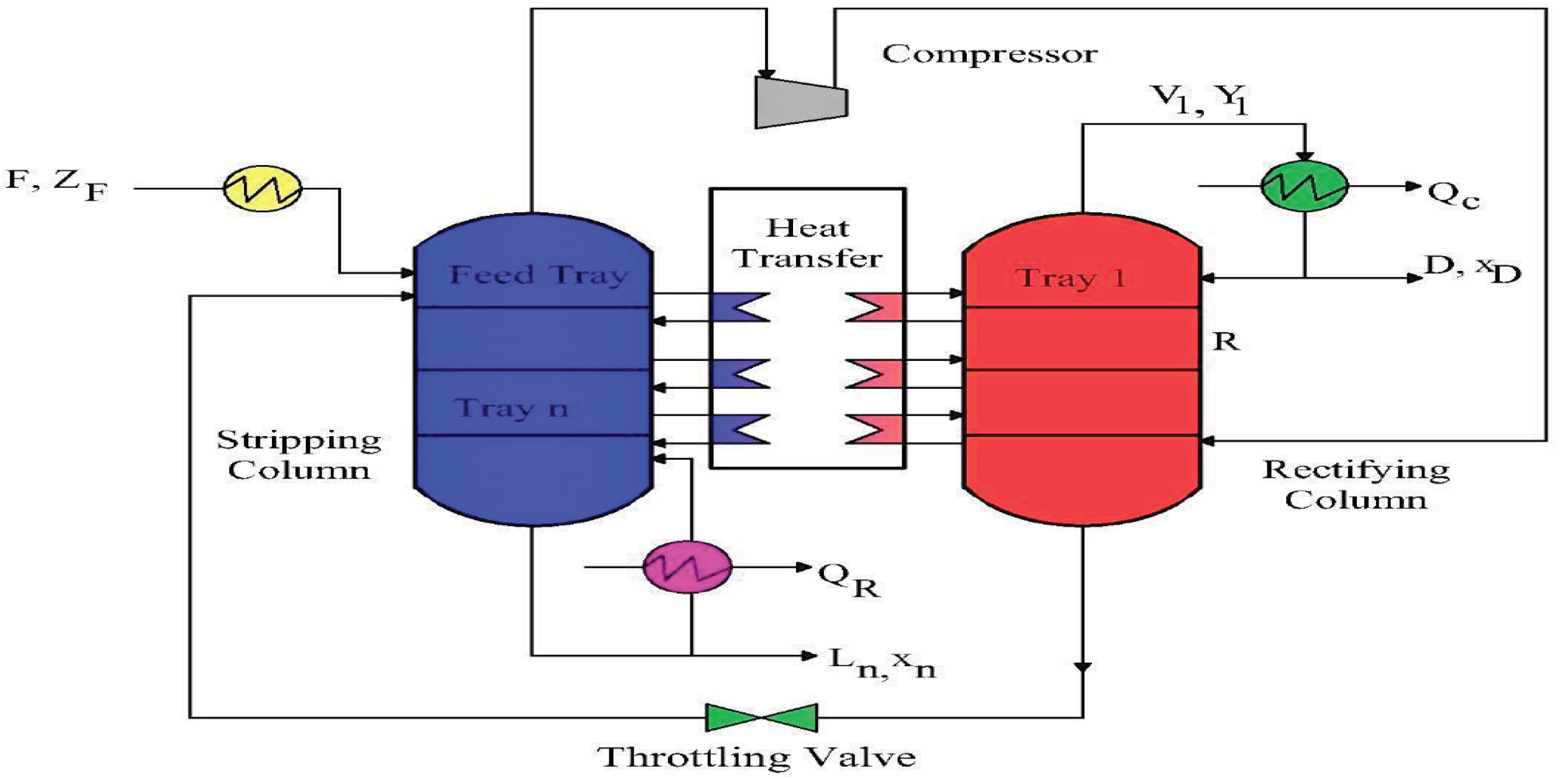
Figure 2.
Block diagram of linear and nonlinear soft sensors.
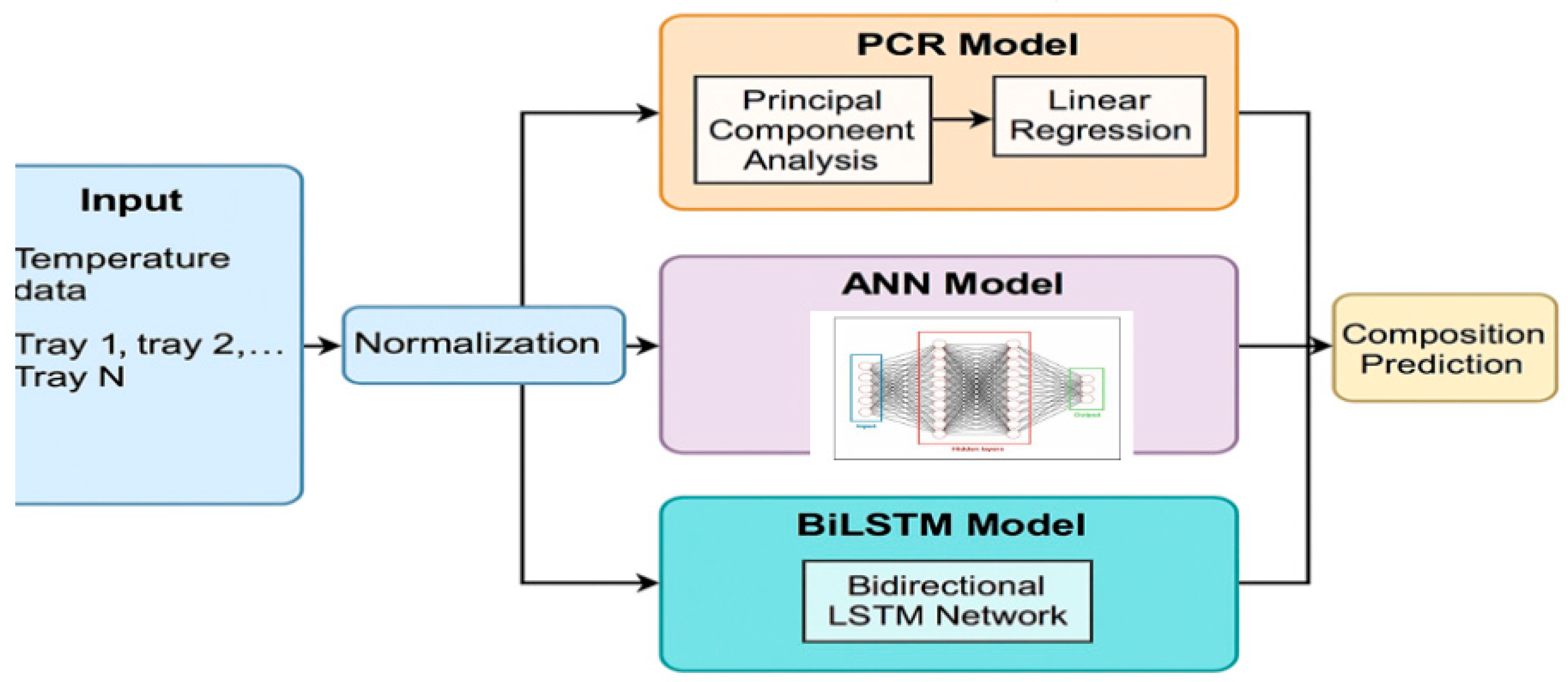
Figure 3.
The block diagram of ANN.
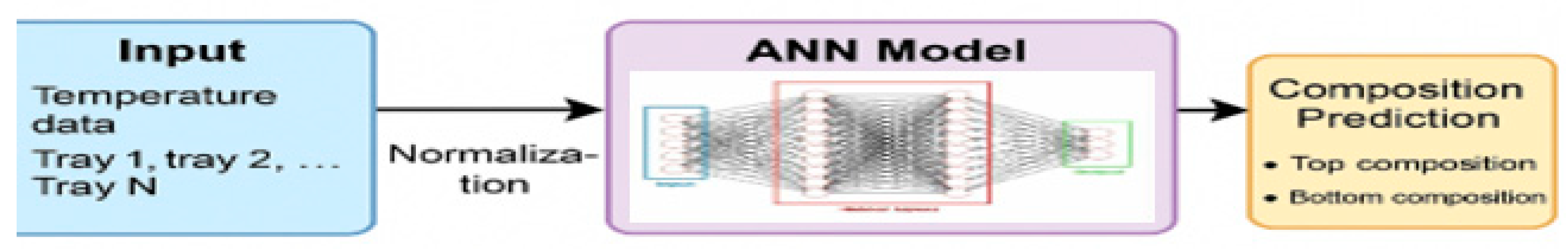
Figure 4.
The architecture of BiLSTM.
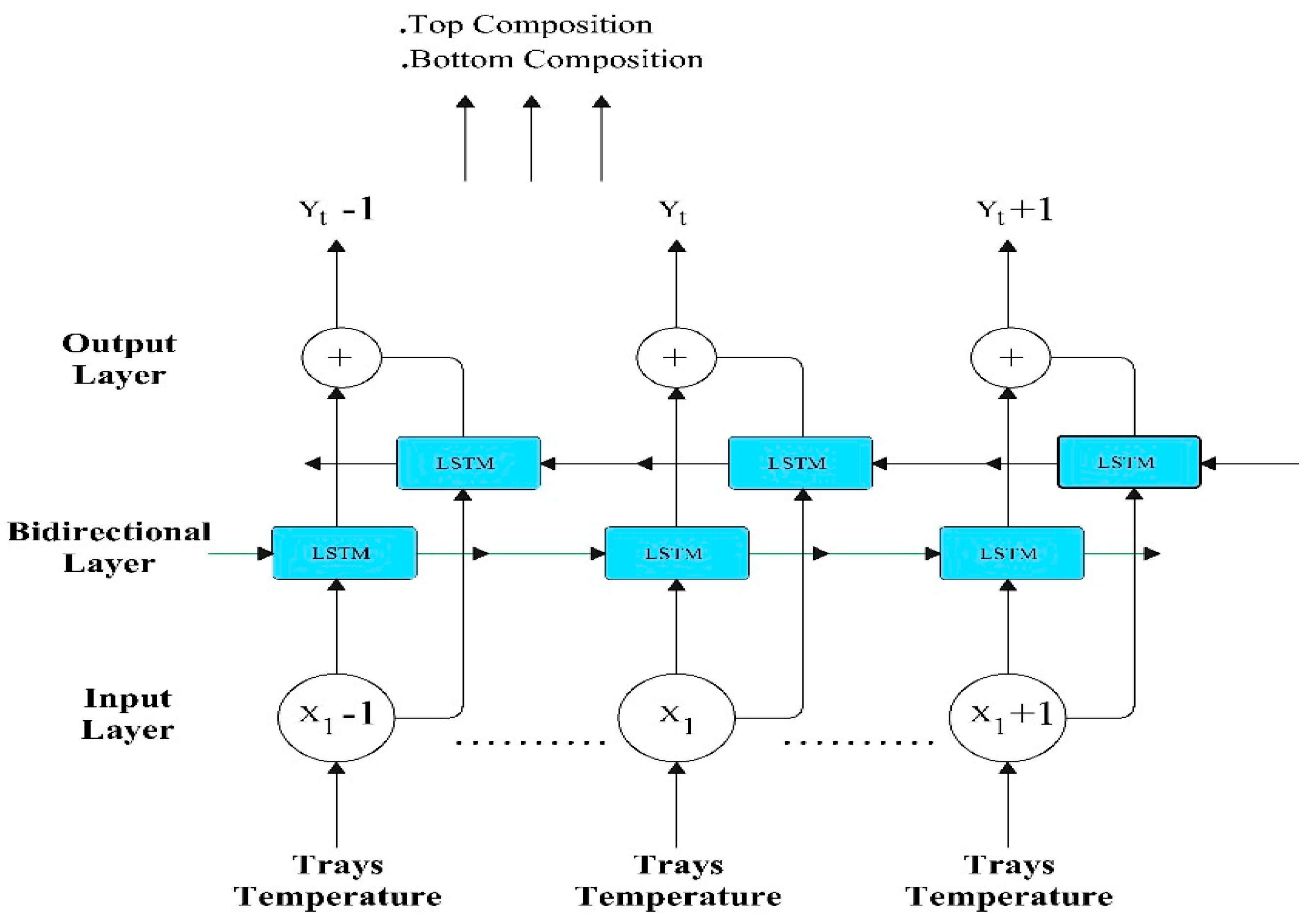
Figure 5.
PCR model performance for top composition.
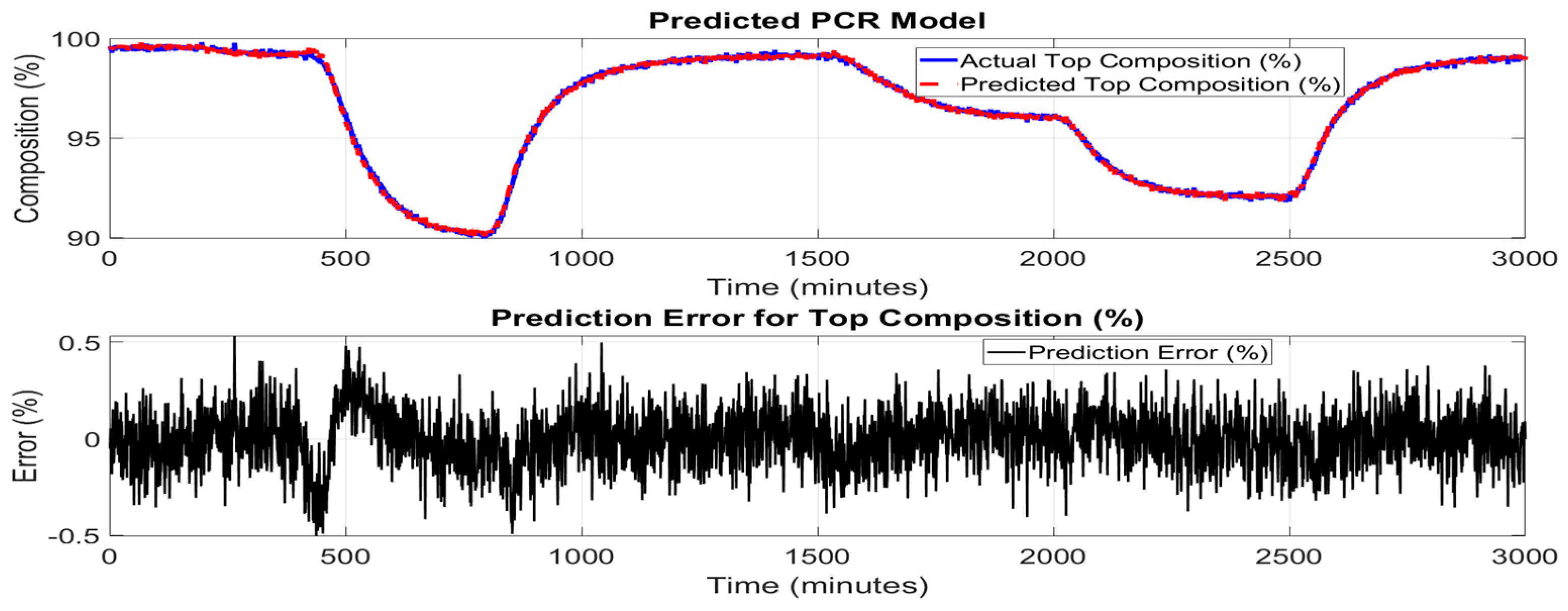
Figure 6.
PCR model performance for bottom composition.
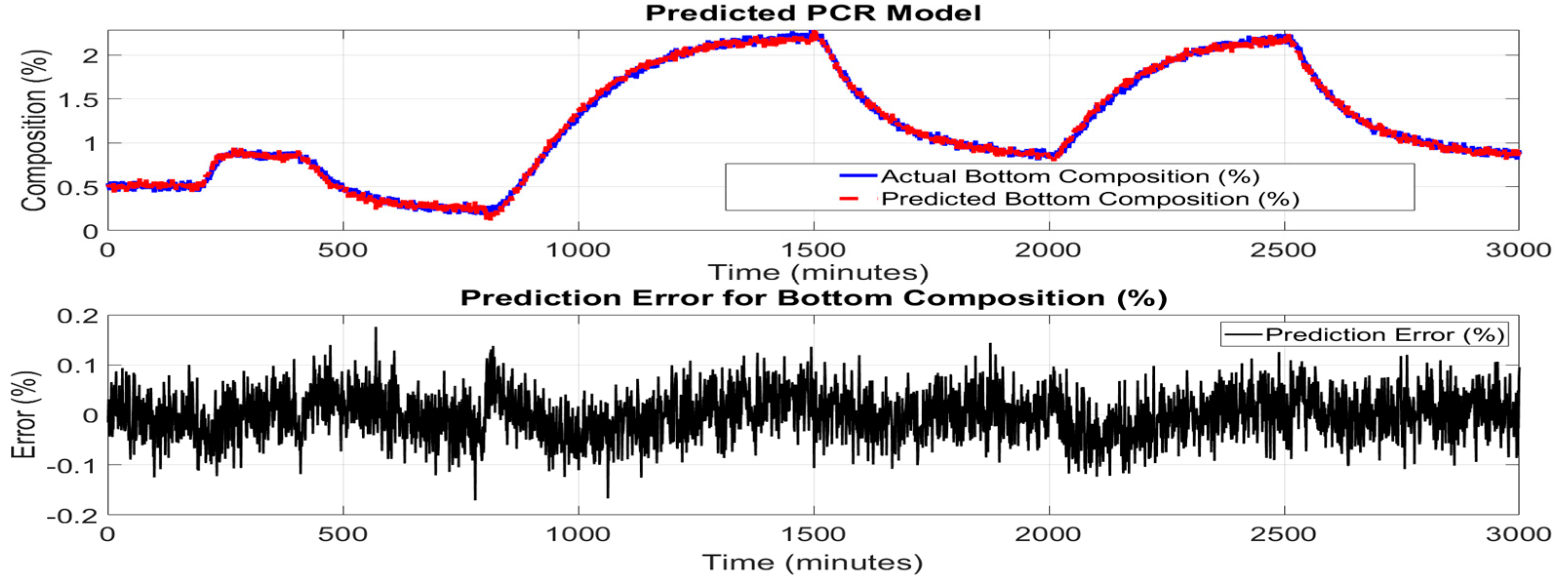
Figure 7.
Top composition ANN model with prediction error.
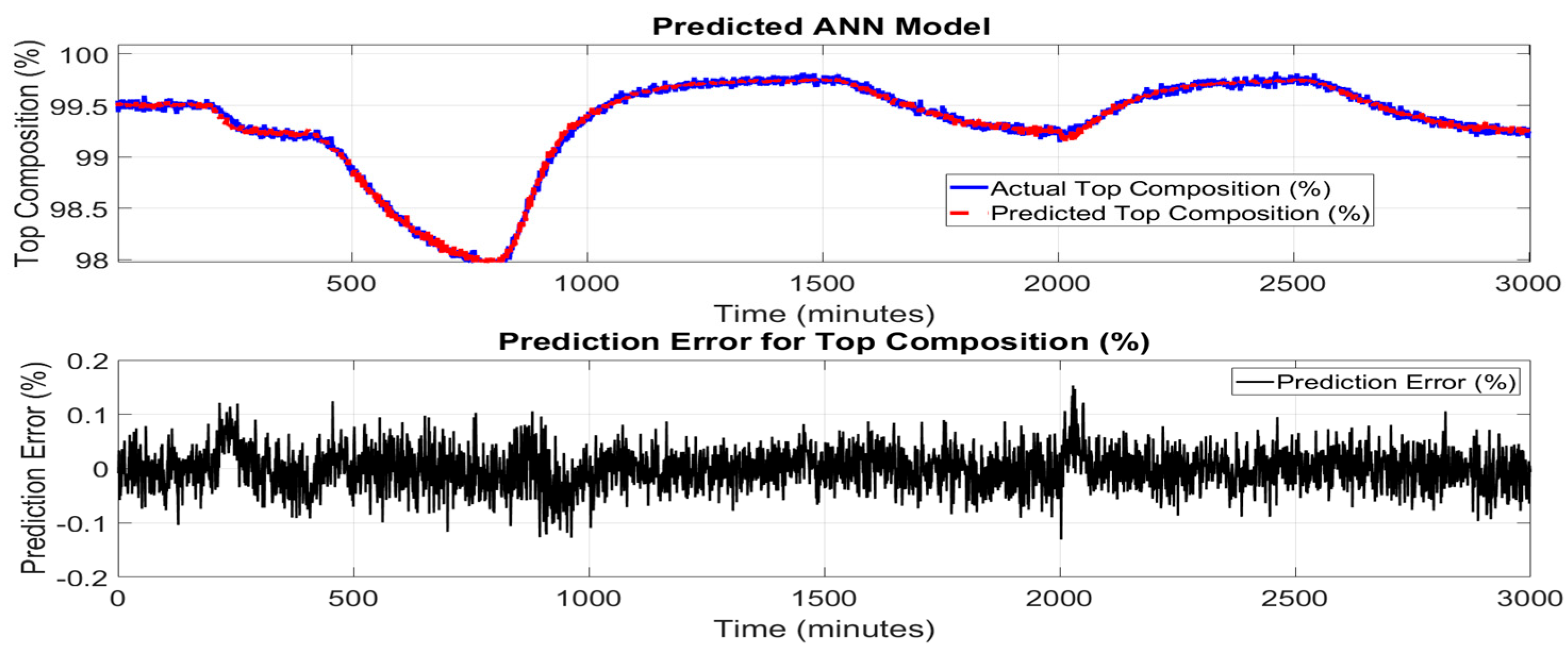
Figure 8.
Bottom composition ANN model with prediction error.
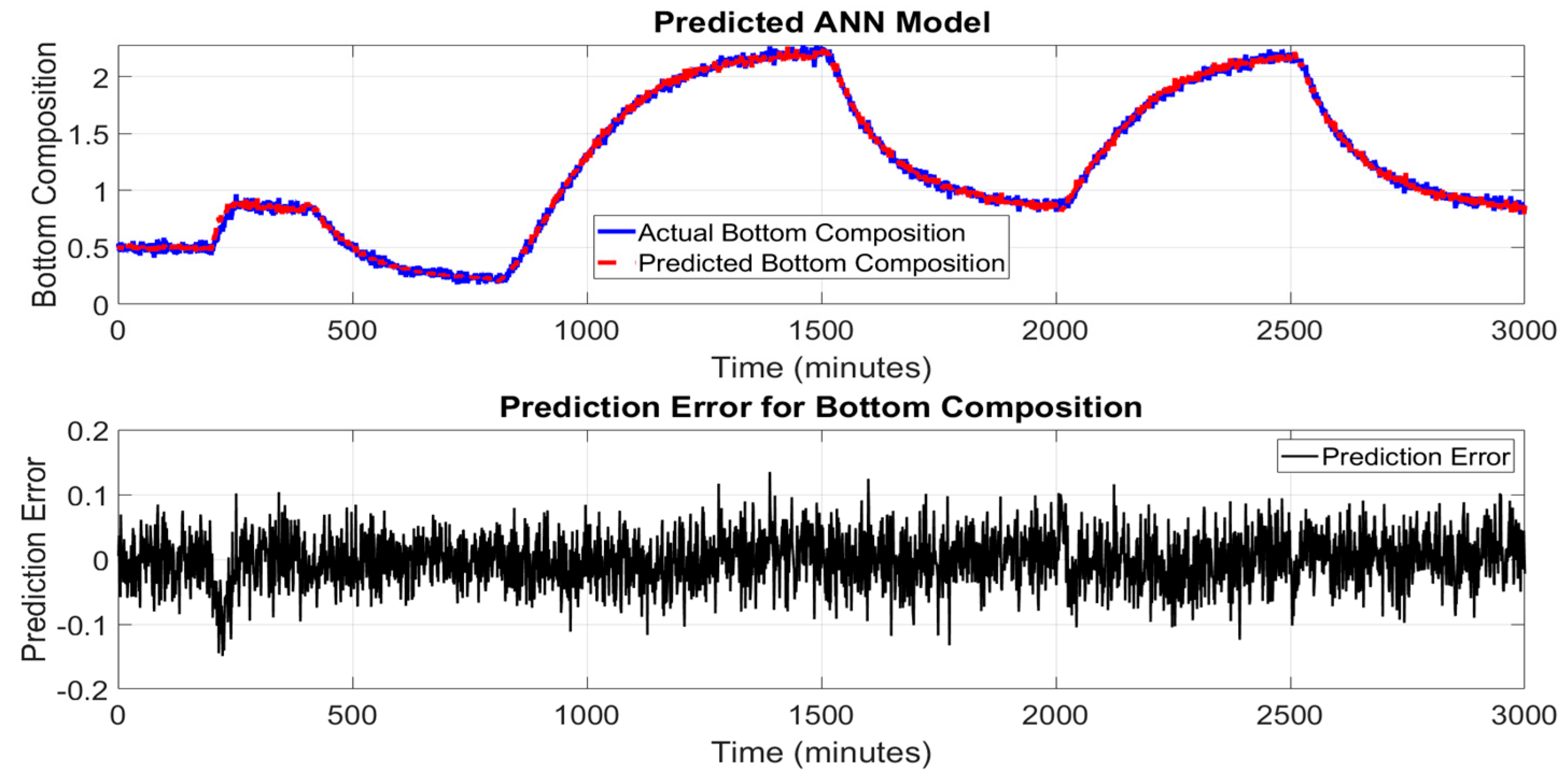
Figure 9.
Top composition BiLSTM model with prediction error.
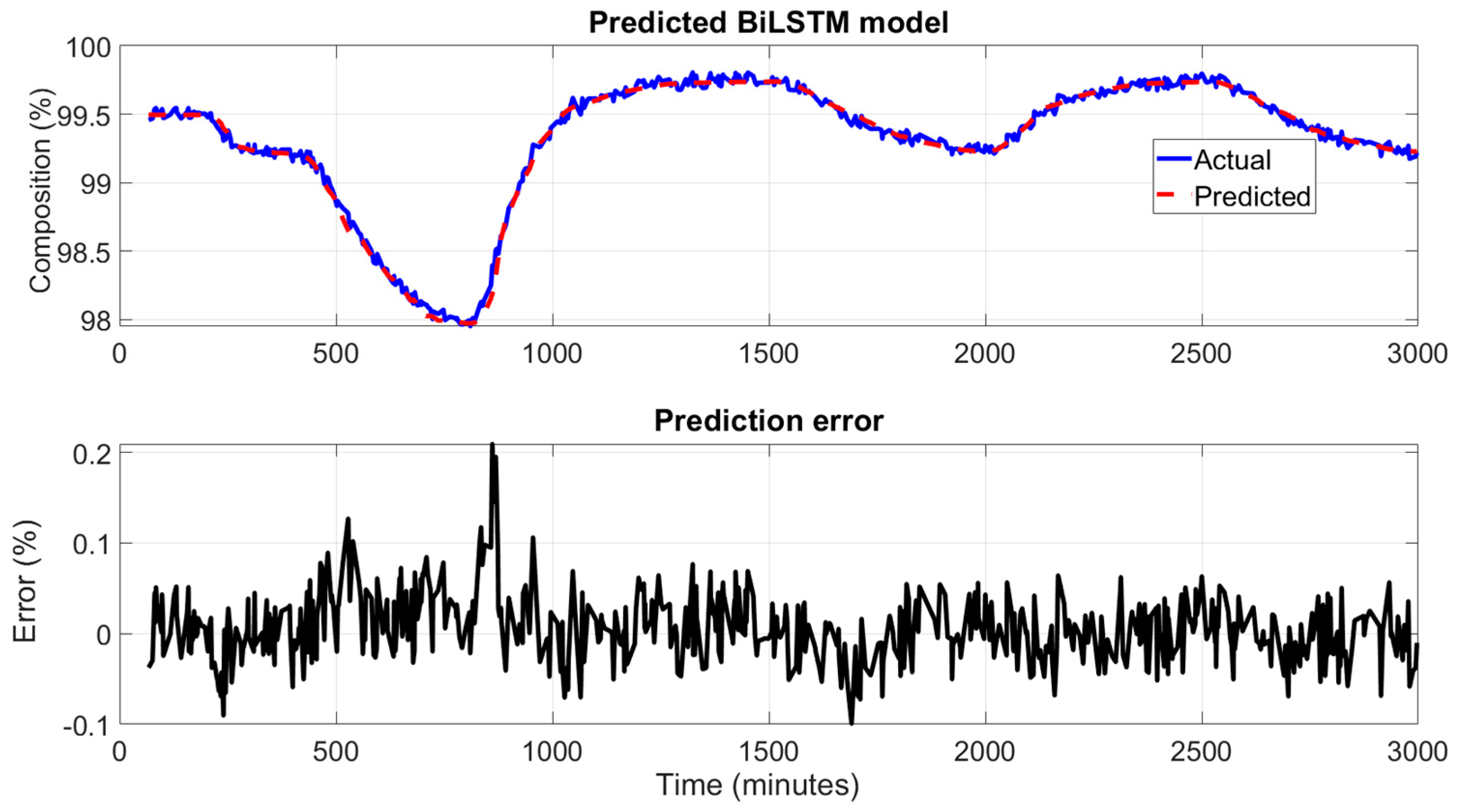
Figure 10.
Bottom composition BiLSTM model with prediction error.
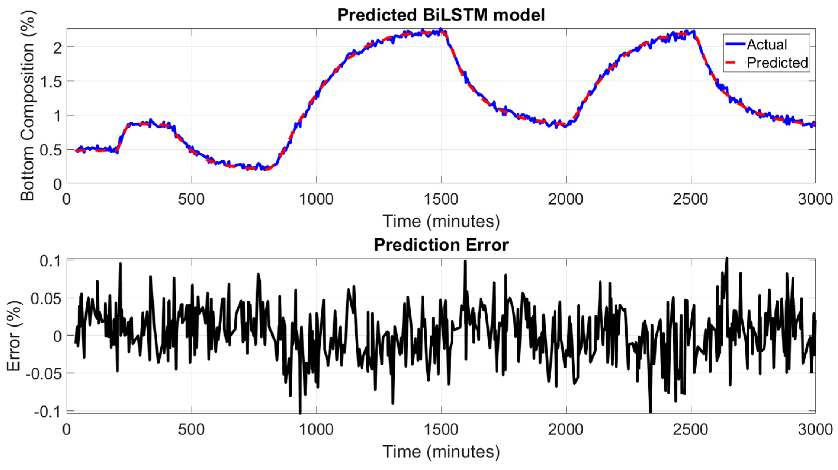
Table 2.
Model Performance Metrics for Top and Bottom Composition Prediction.
| Models | Output | Set | MAE | MSE | R² |
|---|---|---|---|---|---|
| PCR | Top Comp. | Training | 0.00014 | 2.5E-06 | 0.9945 |
| Testing | 0.00016 | 0.000003 | 0.9932 | ||
| Bottom Comp. | Training | 0.00008 | 7E-07 | 0.9959 | |
| Testing | 0.00009 | 0.000001 | 0.9946 | ||
| ANN | Top Comp. | Training | 0.0001 | 1.5E-06 | 0.9968 |
| Testing | 0.00012 | 0.000002 | 0.9958 | ||
| Bottom Comp. | Training | 0.00005 | 6E-07 | 0.9975 | |
| Testing | 0.00007 | 9E-07 | 0.9964 | ||
| BiLSTM | Top Comp. | Training | 0.00007 | 1.2E-06 | 0.998 |
| Testing | 0.00009 | 1.8E-06 | 0.9972 | ||
| Bottom Comp. | Training | 0.00001 | 5E-07 | 0.9991 | |
| Testing | 0.00002 | 4E-07 | 0.9987 |
Disclaimer/Publisher’s Note: The statements, opinions and data contained in all publications are solely those of the individual author(s) and contributor(s) and not of MDPI and/or the editor(s). MDPI and/or the editor(s) disclaim responsibility for any injury to people or property resulting from any ideas, methods, instructions, or products referred to in the content. |
© 2025 by the authors. Licensee MDPI, Basel, Switzerland. This article is an open access article distributed under the terms and conditions of the Creative Commons Attribution (CC BY) license (http://creativecommons.org/licenses/by/4.0/).
Copyright: This open access article is published under a Creative Commons CC BY 4.0 license, which permit the free download, distribution, and reuse, provided that the author and preprint are cited in any reuse.


