
Submitted:
19 June 2025
Posted:
19 June 2025
You are already at the latest version
Abstract
This study aimed to predict the potential habitats of Luciola unmunsana using a species distribution model. Luciola unmunsana is a species found only in South Korea, and its dis-tribution and conservation are relatively poorly studied because females lack wings and are difficult to collect owing to their low mobility. Therefore, we predicted the potential habitats of Luciola unmunsana across South Korea using a single model, maximum entropy (MaxEnt), and a multi-model ensemble model. The points of emergence were based on public data and previous studies from the Jeonbuk Green Environment Support Center (JGESC), Global Biodiversity Information Facility (GBIF), and National Institute of Biolog-ical Resources (NIBR). Among the input variables, the ecoclimate index built through the Shared Socioeconomic Pathways (SSP) scenario-based detailed climate change data was utilized for climate variables, and non-climate variables were built to reflect the ecological characteristics of Luciola unmunsana, such as topography, land cover, and Enhanced Vege-tation Index (EVI). The main findings of this study are summarized below. First, EVI, hy-drological network analysis, land cover, and annual precipitation (Bio12) were found to be influential in predicting potential habitats for Luciola unmunsana in both models. Second, by overlaying the predicted potential habitats and highly significant variables, we found that areas with high vegetation vigor within the forest, proximity to water systems, and relatively high annual precipitation, which can maintain stable humidity, are potential habitats for Luciola unmunsana. Third, field visits and literature surveys to predicted poten-tial habitat sites, including Geumsan-gun, Chungcheongnam-do, Yeongam-gun, Jeolla-buk-do, Mudeungsan, Gwangju-si, Korea, and Gijang-gun, Busan-si, Korea, confirmed the occurrence of Luciola unmunsana. This study is significant because it is the first to construct a national-level species distribution model for Luciola unmunsana, which is declining due to industrialization and urbanization, and to predict potential habitats by applying vari-ous environmental variables reflecting ecological characteristics, thus providing basic da-ta for the conservation and utilization of this emotional insect and environmental indica-tor species. In this study, the spatial resolution of the model was 1 × 1 km for nation-al-level studies. It is necessary to increase the accuracy of the model by including variables with higher spatial resolution when conducting regional-level studies in the future.
Keywords:
Luciola unmunsana
; species distribution model
; MAXENT
; ensemble
; ecoclimate indices
; topographic variables
; EVI
; potential habitat
1. Introduction
Fireflies have long been recognized as emotional insects that are familiar to humans because of their ability to produce light [1]. They are also widely recognized as environmental indicator insects that can only survive in limited habitats and ecologically stable environments, indicating the extent of environmental pollution [1–3]. However, due to reckless development, environmental destruction, ecosystem disturbance, and landscape degradation caused by industrialization and urbanization in modern society, their habitats are being damaged, and their populations and habitat areas are decreasing rapidly [3–5]. In particular, the number and intensity of artificial light sources are increasing, which reduces mutual recognition opportunities between females and males, thereby decreasing the population [5–7]. Consequently, fireflies are increasingly valued as environmental indicators of the extent of environmental pollution and the need for restoration [4].
The most commonly encountered fireflies in South Korea are Luciola lateralis, Lychnuris rufa, and Luciola unmunsana; conservation studies have mainly focused on Luciola lateralis and Lychnuris rufa [8]. Of these, Luciola unmunsana is endemic to South Korea [9] and is difficult to collect because of its lack of inner wings and low mobility in females [6,10]; therefore, there is a relative lack of research on its distribution and restoration compared to other firefly species in South Korea.
Currently, species distribution models are used in various studies, including biodiversity assessment, protected area designation, habitat management and restoration, population or community ecosystem modeling, and climate change prediction [11]. In particular, it provides important information for conservation planning and management by identifying the geographical distribution and properties of populations to identify priority areas to be protected or potentially threatened areas to establish conservation plans and management measures [12,13] Maximum Entropy (MaxEnt), a single model, is effective in modeling the potential distribution of rare and endangered species by performing better in small sample sizes compared to other species distribution modeling methods and is widely used in Korea and abroad because it has the advantage of estimating the ecological status of species with only occurrence information [13,14]. However, when applying single models alone, the accuracy of the models has been questioned because different algorithms of single models lead to different predictions [15]. Therefore, ensemble models that integrate multiple single models have recently been used, and have the advantage of minimizing the shortcomings of single models and maximizing the advantages of reducing their uncertainties of single models [11,13]. Relatedly, a number of studies have been reported that utilize MaxEnt and ensemble models to predict potential habitat for specific species [11,16–20]. However, these prior studies were conducted primarily for endangered or tree-damaging pest species, and few studies have been conducted to predict potential habitats for species with emotional/cultural values and environmental indicator properties, such as fireflies.
Regarding Luciola unmunsana habitat characteristics and restoration, the Daegu Gyeongbuk Research Institute (2012) [21], the Daegu Provincial Environment Agency (2015) [22], and Kim (2015) [8]. Some studies have been conducted by the Jeonbuk Green Environment Support Center (2021) [23], Jeonbuk Green Environment Support Center (2022) [10], and Lim et al. (2022) [24]. However, these studies analyzed specific occurrence points or limited administrative areas, and none were analyzed at a national spatial scale.
Therefore, the aim of this study was to predict the potential habitats of Luciola unmunsana, a major environmental indicator species in South Korea, by creating a species distribution model for the entire country. It is believed that these results can be utilized as basic data for investigating the occurrence of Luciola unmunsana in South Korea.
2. Materials and Methods
The spatial scope of this study was set to South Korea to predict the potential habitats for Luciola unmunsana. The temporal range reflects a 30-year normal climate, which is known to be the optimal sample size for reliable estimates [25].
In addition, we reviewed the environmental factors affecting Luciola unmunsana habitats from previous studies and constructed eco-climatic indices, topographic variables, and land cover maps to reflect them. The spatial resolution of all the variables was unified at 1 km × 1 km to ensure consistency in the analysis.
Potential habitat predictions were analyzed by creating MaxEnt models and ensemble models using MaxEnt 3.4.4 and Rstudio 4.2.1. We analyzed the contribution and significance of the predicted potential habitat and the variables affecting the habitat of Luciola unmunsana, and evaluated the prediction accuracy of both models.
2.1. Building Input
2.1.1. Appearance Point Data
To build a species distribution model, we needed data on the target species' appearance points; in this study, we obtained Luciola unmunsana appearance points from JGESC, GBIF (survey period 2000–2004), and NIBR [26]. In addition, we constructed GPS coordinates of the appearance points presented in previous studies on Luciola unmunsana [8,22], and constructed GPS coordinates of 39 points in total (Figure 1).
2.1.2. Ecological Climate Index
In general, the data for the Ecological Climate Index utilize global-scale input data [27] provided by Worldcilm, Climatologies at high resolution for the Earth’s land surface areas (CHELSA), and global climatologies for bioclimatic modeling (CliMond). However, to improve the accuracy of the analysis, this study utilized ecoclimatic index data based on the shared socioeconomic pathway (SSP) scenario [28] at a 1 km resolution produced by the Korea Rural Development Administration. It was calculated by utilizing 20 indices (Bio01–Bio19) presented by O'Donnell and Ignizio (2012) [29] (Table A1); as the temporal range of this study was set to 1981–2010, the analysis was conducted using the ecological climate index data for that period.
When modeling using the Ecological Climate Index, a high correlation between variables can reduce efficiency and adversely affect the interpretation of results [30,31]. Therefore, to account for the correlation between variables, multicollinearity was removed through an analysis using Pearson's correlation coefficient. This is the most widely used statistic to measure the correlation between variables on an equivalence/ratio scale [32]. In this study, multicollinearity was removed by using Pearson's correlation coefficient in RStudio 4.3.3 to exclude variables with a high correlation of ±0.85 or higher, resulting in the selection and analysis of Bio01, Bio02, Bio04, Bio12, Bio14, and Bio15.
2.1.3. Terrain Variables
In general, fireflies occur at high densities in low-slope sites [22]. These slopes are less prone to soil runoff, allowing the accumulation of organic matter and moisture, which can lead to diverse vegetation [19]. In particular, fireflies prefer dark and shady environments and thrive in areas with diffused light or short periods of sunlight [21]. Luciola unmunsana is also generally found in terrains where stable humidity can be maintained, such as forest edges on gentle slopes, which tend to be located near water resources, such as streams and ponds, or around broadleaf forest stands with multi-layered vegetation that are often associated with agricultural ditches and streams [22,24,33]. Terrestrial snails, the main food source for Luciola unmunsana, are found in shady forests with little direct sunlight or stable humidity [23].
Therefore, a Digital Elevation Model (DEM) with a resolution of 90m×90m was constructed in CGIAR-CSI [34] to construct non-climatic variables affecting the habitat of Luciola unmunsana, followed by slope and shade gradient analysis, and a water network analysis map was constructed using the Environmental Big Data Platform [35] to construct variables on distance to water systems.
2.1.4. Land Cover Map
To reflect the land cover and use in Korea, we used WorldCover V2 2021, a 10m x 10m spatial resolution land cover map provided by the European Space Agency (ESA) [36]. It is based on Sentinel-1 and Sentinel-2, and has an overall accuracy of 76.7% [37].
The results of the Daegu Provincial Environment Agency (2015) [22] showed that Luciola unmunsana occurred mainly in coniferous forests with mixed broadleaf trees, and in areas dominated by coniferous forests. In addition, Luciola unmunsana is found in broadleaf forests, but its food source is also found in forests such as bamboo forests and coniferous forests [10]. Therefore, in this study, we utilized the map for tree cover among the classified items and included data for non-forested areas, because it is believed that the response of potential habitats in non-forested areas will also affect the prediction of potential habitats in forested areas.
2.1.5. Enhanced Vegetation Index (EVI)
As vegetation develops, dead leaves and octopuses accumulate on the surface, and microorganisms in the soil decompose them, increasing the organic matter content [22]. This increases water retention during rainfall, creating conditions for Luciola unmunsana larvae to live under fallen leaves, octopuses, organic matter layers, and stones [22]. Therefore, in this study, the Vegetation Index (VI) was additionally entered to reflect information on vegetation abundance and vegetation vigor in the species distribution model.
The EVI is an index developed to correct for atmospheric conditions, water pipe effects, and areas with high vegetation density and provides an improved vegetation index using atmospheric correction factors, water pipe correction factors, and blue light values [38]. Compared to the Normalized Difference Vegetation Index (NDVI), it reduces errors due to atmospheric residuals and can be used more effectively in seasonal and process-based models of forest vegetation [39–41]. Therefore, in this study, EVI was used to construct a species distribution model.
To construct the EVI, we used monthly averaged values for 2022 from Moderate Resolution Imaging Spectroradiometer (MODIS) [42,43] satellite imagery.
2.2. Creation of Species Distribution Models
2.2.1. MaxEnt
The MaxEnt model is a machine learning model based on the Maximum Entropy Approach, first introduced by Berger et al. (1996) [44], which can estimate values by maximizing incomplete data [19] and shows high accuracy compared to other species distribution models that use only species occurrence data [45–47]. It is also commonly used in species distribution modeling because it represents linear non-parametric relationships between variables [48,49].
Although the parameters are set by default within MaxEnt, this does not always result in an optimal model, and can result in a suboptimal model [50,51]. Therefore, it is necessary to analyze the complexity of the model with different combinations of parameters to select a combination with a lower complexity for modeling and optimizing the model. Two main selectable parameters affect the model performance: Feature Class (FC) and Regularization Multiplier (RM) [52]. FC refers to a set of mathematical transformations of the independent variables used in the model to optimize the model, and there are five types: Linear (L), Quadratic (Q), Product (P), Hinge (H), and Threshold (T) [48,53]. RM is a numerical parameter that controls the strength of the FC used in the model and can reduce or increase the ease of modeling [54,55]. The Akaike information criterion (AIC) value is a statistic that quantifies the degree of discrepancy between the true and candidate models, reflecting the fit and complexity of the model; the model with the minimum AICc value, delta AICc, equal to zero, is considered the best model [56,57].
In this study, 60 models were generated using six FCs (L, LQ, H, LQH, LQHP, and LQHPT) and 10 RMs (0.5, 1, 1.5, 2, 2.5, 3, 3.5, 4, 4.5, and 5). In addition, MaxEnt 3.4.4 and ENMeval packages were run together in Rstudio, K-fold was performed 10 times, and the model with a delta AICc value of '0' was finally selected.
In the modeling settings, FC was selected as LQHP, RM was selected as 3, and 'Replicated run type' was set to 'Bootstrap' and repeated 10 times.
The maximum number of background points was set to 10,000, which was typically set to 10,000 if there were more than 10,000 background points [58]. In this study, 98,928 potential background points were identified as available within the spatial scope of the study; therefore, they were set to 10,000, and the results were outputted using logistic output.
2.2.2. Ensemble Model
Ensemble models are a recently developed method for predicting species distributions that combine multiple algorithms and statistical models to reduce the uncertainty of a single model. It has been proposed to improve outcomes such as predicting the current distribution of species, patterns of species richness, and species diversity [11,59,60]. It has the advantage of providing a variety of validation methods for the model that can overcome the shortcomings of other commonly used models, and is currently widely used [60].
To create an ensemble model for predicting the potential habitats of Luciola unmunsana, Rstudio 4.3.3 to conduct the analysis. The Biomod2 package was utilized within Rstudio 4.3.3, and in this study, 39 emergence sites were used as background data to generate pseudo-absence data containing 1000 non-emergence sites.
We used six individual models to build the ensemble model: GLM, GBM, CTA, FDA, MARS, and RF among the models provided by Biomod2. The selected models require the input of non-abundance and abundance data and are known to be more accurate than models based on abundance data alone [13].
2.3. Model Accuracy Verification
2.3.1. MaxEnt Model Accuracy Verification
To verify the accuracy of the MaxEnt model, an AUC test was performed. The AUC is a measure of whether a true value is predicted by a true value or whether a false value is predicted by a true value, and the accuracy is measured using the AUC value of the ROC curve [17,61]. In general, AUC values are interpreted as 0.5-0.6 (failure), 0.6-0.7 (no value), 0.7-0.8 (poor), 0.8-0.9 (good), and <0.9 (excellent) [62].
2.3.2. Ensemble Model Accuracy Verification
Kappa, TSS, and AUC validations were performed to verify the accuracy of the ensemble models. Kappa is used to determine the overall accuracy of model predictions by correcting the possibility of classification matching by chance. It is mainly used to validate the accuracy of occurrence and non-occurrence data [11]. In particular, it is widely used as a means of validating models in ecology and validating the accuracy of land-cover classification using satellite imagery [11,63]. The value of the coefficient ranges between -1 and 1, with values of 0.2 or less indicating poor agreement, values of 0.21 to 0.4 indicating moderate agreement, values of 0.41 to 0.6 indicating moderate agreement, values of 0.61 to 0.8 indicating high agreement, and values of 0.81 to 1 indicating perfect agreement [64].
The TSS value includes an assessment of the accuracy of both the occurrence and non-occurrence data. Unlike the AUC, it is not dependent on the distribution area or shape of the target species and is therefore often used to validate species distribution models [63]. A TSS coefficient value of 0.4 to 0.6 indicates 'moderate agreement', 0.6 to 0.7 indicates 'high agreement', and 0.7 or higher indicates 'near agreement' [12].
3. Results
3.1. Model Potential Habitat Prediction Results
3.1.1. MaxEnt Model Potential Habitat Prediction Results
To create a binomial map showing suitable and unsuitable habitats, the model was thresholded through the 'Maximum training sensitivity plus specificity logistic threshold' value, and the threshold value was 0.5872. After setting this threshold value using QGIS S/W 3.30.3, a binomial map was created and masked with a map of tree cover from the land cover map to predict potential habitats in the forest area (Table 1). The total area of potential habitat for Luciola unmunsana predicted using the MaxEnt model was 8,785 km2 (Table 2). The potential habitats are in the following order: Jeollanam-do, Gyeongsangbuk-do, and Gyeongsangnam-do.
3.1.2. Ensemble Model Potential Habitat Prediction Results
To create a binomial map of the ensemble model, a probability map with values ranging from 0 to 1000 was thresholded. The threshold value that maximized the TSS value was used, and the threshold value was derived as '659. ’ A bimodal map was created using QGIS S/W 3.30.3 as MaxEnt and masked with the map of tree cover from the land cover map to predict the potential habitat in the forest area (Table 1). The total area of potential habitat for Luciola unmunsana predicted using the ensemble model was 6,971 km2 (Table 2). Compared with the MaxEnt model, a relatively small area of potential habitat was predicted, and the main areas of potential habitat were Jeollanam-do, Jeollabuk-do, and Gyeongsangbuk-do, with Jeollanam-do as the new top distribution area.
3.2. Contribution and Significance Analysis Results by Model Variable
3.2.1. Results of Contribution and Significance Analysis by MaxEnt Model Variables
When analyzing the contribution of each variable in the model, the land cover map contributed the most (26%), followed by the EVI (25.1%), water network analysis (21.9%), and Bio12 (11.6% (Table A4). In terms of importance, EVI had the highest contribution at 34%, followed by land cover (23.7 %), water network analysis (19.9 %), and Bio12 (6.6 %).
Among the response curves of each variable, the EVI, land cover, water network analysis, and Bio12 were the most important (Table 3). The EVI response curve showed that the response gradually increased as vegetation vigor increased, and the response curve of the water network analysis showed that the response gradually decreased as the distance from the water system increased. In addition, the response curve of the land-cover map showed that the response was relatively higher in forested areas than in non-forested areas, and the response curve of Bio12 showed that the response increased as annual precipitation increased.
3.2.2. Importance Analysis Results by Ensemble Model Variable
The importance of each variable in the built model was the highest for EVI (39.3%), followed by water network analysis (25.6%), Bio12 (10.1%), and land cover (8.3% (Table A4).
3.3. Model Accuracy Validation Results
3.3.1. MaxEnt Model Accuracy Validation Results
To determine the accuracy of the MaxEnt model implemented in this study, we used the AUC test to determine potential habitat prediction performance (Figure 2). The accuracy of the AUC test was 0.810, which is’ good, indicating that the MaxEnt model implemented in this study had a relatively good prediction performance.
3.3.2. Ensemble Model Accuracy Validation Results
To evaluate the potential habitat prediction performance of the ensemble model implemented in this study, Kappa, TSS, and AUC values were used to determine the accuracy (Table 4). The Kappa value was 0.741, which indicates a high degree of agreement; the TSS value was 0.808, which indicates near agreement; and the AUC value was 0.961, which indicates excellent prediction performance, indicating that the ensemble model has a high level of prediction performance.
3.4. Key Variables and Potential Habitat Nesting Results
The variables with the highest importance in both models were the EVI, hydrographic network analysis, land-cover maps, and Bio12. Therefore, the potential habitat area predicted by the model was analyzed by overlaying the key variables with the predicted potential habitat area using the model with the key variables with the highest importance in both models.
3.4.1. EVI and Predictive Potential Habitat Overlap Area Analysis
We overlaid the EVI with the predicted potential habitats from the MaxEnt and ensemble models (Table 5) and found that both models predicted relatively large areas of potential habitats within the 0.4-0.5 range of vegetation vigor (Table 6). Values of EVI range from -1 to +1, and values in the 0.4-0.5 range are generally considered to be areas of intermediate vigor and density of vegetation, which can be categorized as low light forests with an understory vegetation [65]. These results are consistent with the ecological characteristics of Luciola unmunsana, which prefers forest edges or low-light forests where understory vegetation is developed and humidity remains stable [22,24,33].
3.4.2. Hydrographic Maps and Predictive Potential Habitat Overlap Analysis
Based on the results of the water network analysis, we overlaid the predicted potential habitat from the MaxEnt and ensemble models (Table 7) and found that both models predicted relatively large areas of potential habitat within a range of 0-100 m distance to water (Table 8). These results suggest that proximity to water resources is an important environmental factor for Luciola unmunsana. Areas in close proximity to water systems have stable soil and air humidity, which is consistent with Luciola unmunsana's preference for moist environments [22,24,33]. These areas may also provide suitable conditions for the colonization of land snails, the main food source for Luciola unmunsana, which may contribute to the maintenance of stable populations of Luciola unmunsana.
3.4.3. Bio12 and Predictive Potential Habitat Overlap Area Analysis
4. Discussion
This study utilized a single model, MaxEnt, and a multiple model, an ensemble model, to predict the potential habitats of Luciola unmunsana. Importance analysis of the variables in both models showed that the EVI, land cover, hydrological network analysis, and annual precipitation (Bio12) were highly important. The response curve analysis of each variable showed that the response value of the EVI increased with increasing vegetation vigor, and the water network analysis showed that the response increased with increasing distance from the water system. In the case of land-cover maps, the response was higher in forested areas than in non-forested areas, and the response increased as annual precipitation increased.
Overlaying the highly significant variables with the predicted potential habitat, the EVI was 0.4 to 0,5, the distance from the water bodies was 0–100 m, and the annual precipitation was 1,500 mm–2,000 mm. Taken together, these results suggest that the most suitable areas for Luciola unmunsana are those with forested vegetation and relatively close proximity to water systems, where humidity is stable.
The predicted area of the potential habitat was found to be lower in the ensemble model (6,971㎢ compared to 8,785㎢ in the MaxEnt model. This result was likely due to the tendency of the MaxEnt model to overestimate potential habitats, as in previous studies [66,67], and the fact that the ensemble model only identified potential habitats where the predictions of all six models were used to build the model overlap.
5. Conclusions
The aim of this study was to predict the potential habitats of Luciola unmunsana, a major environmental indicator species in South Korea. To this end, we constructed the occurrence points of Luciola unmunsana and predicted potential habitats using MaxEnt and ensemble models for South Korea. To predict potential habitats, we reviewed the main environmental factors that affected the habitat of Luciola unmunsana in previous studies and constructed them as variables for analysis. Subsequently, the contribution and significance of the variables were evaluated, and the prediction accuracy of the two models was verified.
The main findings of this study are as follows. First, both models showed that EVI, hydrological network analysis, land cover, and annual precipitation (Bio12) were relatively influential in predicting Luciola unmunsana potential habitats. The response curve analysis of MaxEnt showed that the response value increased as the EVI increased, and the response tended to increase with increasing distance from the water system. In the case of the land cover map, the response was higher in forested areas and the response value increased with higher annual precipitation.
Second, we overlaid the predicted potential habitats with variables that showed high importance in determining their distribution and found that areas with high vegetation vigor within the forest, close proximity to water systems, and relatively high annual precipitation, which allows humidity to remain stable, were analyzed as potential habitats for Luciola unmunsana. These results are consistent with the ecological characteristics of Luciola unmunsana, which prefers forest edges or low-light forests with developed understory vegetation and stable humidity [22,24,33], as well as the habitat characteristics of its main food source, terrestrial snails [23].
Third, field visits and literature surveys of sites predicted as potential habitats, but not existing sites, such as Geumsan-gun, Chungcheongnam-do, Yeongam-gun, Jeollanam-do, Mudongsan Mountain, Gwangju-si, Gwangju, and Gijang-gun, Busan, confirmed the occurrence of Luciola unmunsana. As a result of the model accuracy verification, the MaxEnt model was evaluated as 'good, ’ with an AUC value of 0.810. In addition, the ensemble model was evaluated as 'good' with a Kappa value of 0.741, a TSS value of 0.808, and a near agreement level, and the AUC value of 0.961 was evaluated as 'excellent. ’ Therefore, the potential habitat prediction results of this study were reliable based on the relatively high model accuracy, and we believe that key habitats were predicted even in areas where no emergence points were entered.
This study is significant in that it is the first to establish a national-level species distribution model for Luciola unmunsana, which is declining owing to industrialization and urbanization, and to predict potential habitats by applying various environmental variables reflecting ecological characteristics, thereby providing basic data for the conservation and utilization of Korea's major emotional insect and environmental indicator species. In particular, it can be utilized as basic data for academic and practical use because it derives more reliable prediction results by combining a single model, MaxEnt, and a multiple-model, ensemble model. However, to improve the ease and accuracy of future species distribution models, it will be necessary to build additional emergence point data and utilize them for model construction. In addition, the spatial resolution was re-projected to 1 km × 1 km to analyze South Korea. Consequently, a single pixel may contain various environmental and topographical characteristics, and some details may have been lost. Therefore, future studies with regional spatial coverage may need to input variables with higher spatial resolutions to improve the precision and predictive power of the model.
Author Contributions
Conceptualization, S.-W.K.; Methodology, S.-W.K.; Validation, S.-W.K.; Data interpretation, S.-W.K.; Writing—review & editing, S.-W.K.; Software, B.-J.J. and J.-Y.L.; Literature search, B.-J.J. and J.-Y.L.; Resources, B.-J.J.; Visualization, B.-J.J.; Data analysis, B.-J.J.; Formal analysis, J.-Y.L.; Writing—original draft, B.-J.J. and J.-Y.L. All authors have read and agreed to the published version of the manuscript.
Funding
This Study was supported by the 2024 research fund from Wonkwang University.
Conflicts of Interest
The authors declare no conflict of interest.
Appendix A

Table A1.
Ecological Climate Index List (O'Donnell and Ignizio, 2012) [23].
| Separation | Description | Unit |
| Bio01 | Average annual temperature | ℃ |
| Bio02 | Average daily temperature range | ℃ |
| Bio03 | Isothermality | % |
| Bio04 | Temperature seasonality (standard deviation) | ℃ |
| Bio04a | Temperature seasonality (CV) | % |
| Bio05 | Highest temperature in warmest month | ℃ |
| Bio06 | Lowest temperature in the coldest month | ℃ |
| Bio07 | Annual temperature range | ℃ |
| Bio08 | Average temperature in the wettest quarter | ℃ |
| Bio09 | Average temperature of the driest quarter | ℃ |
| Bio10 | Average temperature in warmest quarter | ℃ |
| Bio11 | Average temperature of the coldest quarter | ℃ |
| Bio12 | Annual precipitation | ㎜ |
| Bio13 | Precipitation in the wettest month | ㎜ |
| Bio14 | Precipitation in the driest month | ㎜ |
| Bio15 | Precipitation seasonality | % |
| Bio16 | Precipitation in wettest quarter | ㎜ |
| Bio17 | Dryest quarter precipitation | ㎜ |
| Bio18 | Precipitation in warmest quarter | ㎜ |
| Bio19 | Coldest quarter precipitation | ㎜ |
Appendix B
Table A2.
MaxEnt and Ensemble Model Potential Habitat Key Predicted Regions.
| Models | Metropolitan City- State | City - County - District |
| MaxEnt | Gangwon-do | Yangyang-gun |
| Gyeonggi-do | Gapyeong-gun, Yangpyeong-gun | |
| Chungcheongbuk-do | Yeongdong-gun | |
| Chungcheongnam-do | Geumsan-gun | |
| Jeollabuk-do | Muju-gun, Wanju-gun, Jinan-gun | |
| Jeollanam-do | Gangjin-gun, Gwangyang-si, Damyang-gun, Boseong-gun, Suncheon-si,Yeongam-gun, Jangseong-gun, Jangheung-gun | |
| Gyeongsangbuk-do | Mungyeong City, Cheongdo County, Cheongsong County, Pohang City | |
| Gyeongsangnam-do | Yangsan-si, Hadong-gun | |
| Ulsan Metropolitan City | Ulju-gun | |
| Busan Metropolitan City | Gijang-gun | |
| Ensemble | Gangwon-do | Hwacheon-gun |
| Chungcheongbuk-do | Yeongdong-gun, Okcheon-gun | |
| Chungcheongnam-do | Geumsan-gun, Nonsan-gun | |
| Jeollabuk-do | Muju-gun, Sunchang-gun,Wanju-gun, Jinan-gun | |
| Jeollanam-do | Gwangyang-si, Gurye-gun, Naju-si,Damyang-gun, Yeongam-gun,Jangseong-gun, Jangheung-gun | |
| Gwangju Metropolitan City | Dong-gu | |
| Gyeongsangbuk-do | Cheongdo-gun | |
| Gyeongsangnam-do | Goseong-gun, Yangsan-si, Hadong-gun | |
| Ulsan Metropolitan City | Ulju-gun | |
| Busan Metropolitan City | Gijang-gun |
Appendix C
Table A3.
Contribution and Importance of MaxEnt Variables.
| Input variables | Percentage contribution (%) | Permutation Importance (%) |
| Bio01 | 0.9 | 1.4 |
| Bio02 | 0.3 | 0.2 |
| Bio04 | 4.5 | 6.5 |
| Bio12 | 11.6 | 6.6 |
| Bio14 | 4.2 | 4.0 |
| Bio15 | 1.8 | 1.0 |
| Slope | 2.2 | 0.7 |
| Shaded Corridor | 1.4 | 2.1 |
| Hydrologic Network Analysis Map | 21.9 | 19.9 |
| Land cover map | 26.0 | 23.7 |
| EVI | 25.1 | 34.0 |
Table A4.
Importance by the ensemble model variable.
| Input variables | Permutation Importance (%) |
| Bio01 | 5.4 |
| Bio02 | 0.8 |
| Bio04 | 1.6 |
| Bio12 | 10.1 |
| Bio14 | 1.0 |
| Bio15 | 1.8 |
| Slope | 5.3 |
| Shaded Corridor | 0.8 |
| Hydrologic Network Analysis Map | 25.6 |
| Land cover map | 8.3 |
| EVI | 39.3 |
Figure 1.
Luciola unmunsana Appearance point
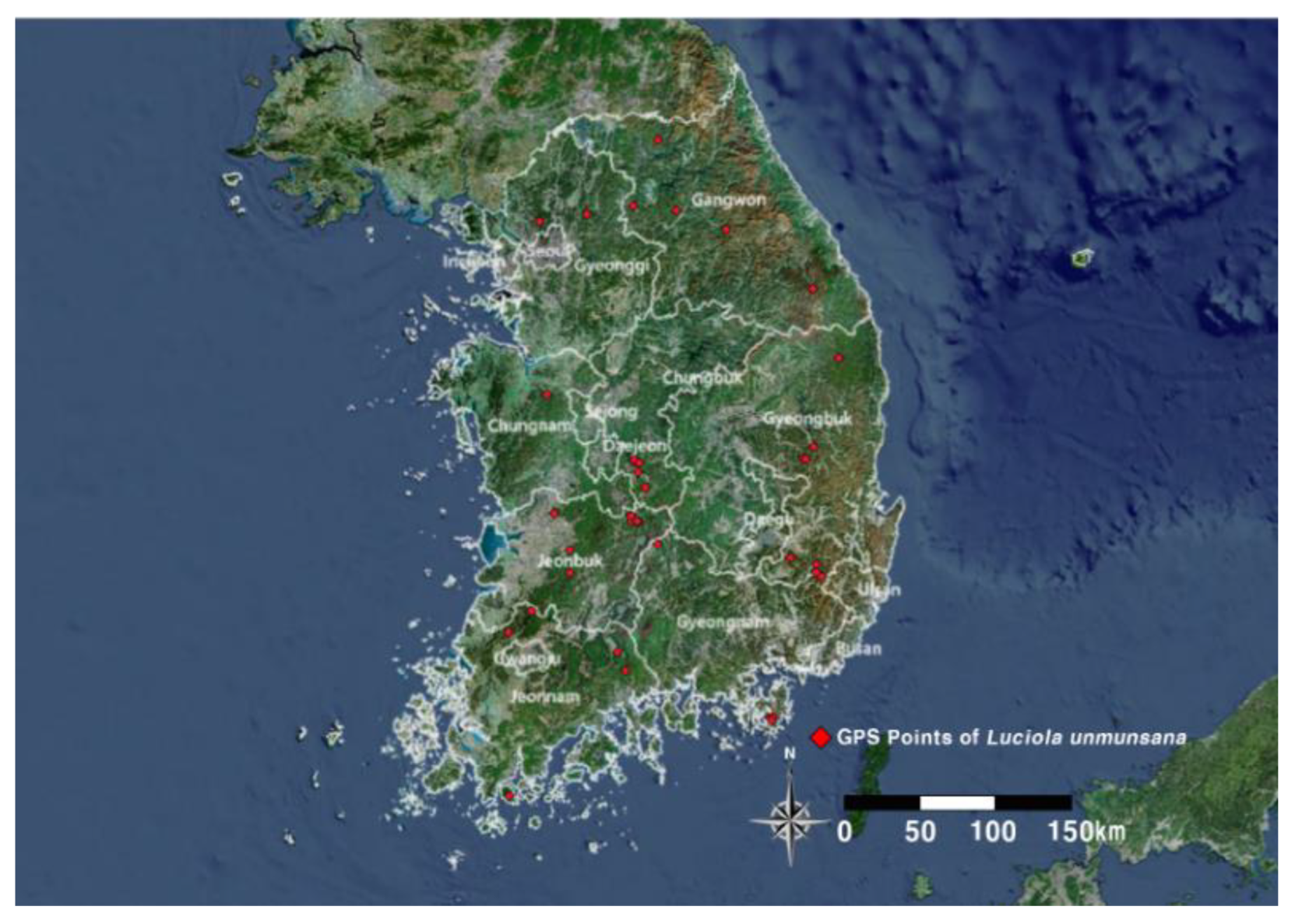
Figure 2.
MaxEnt Model AUC Validation Results.
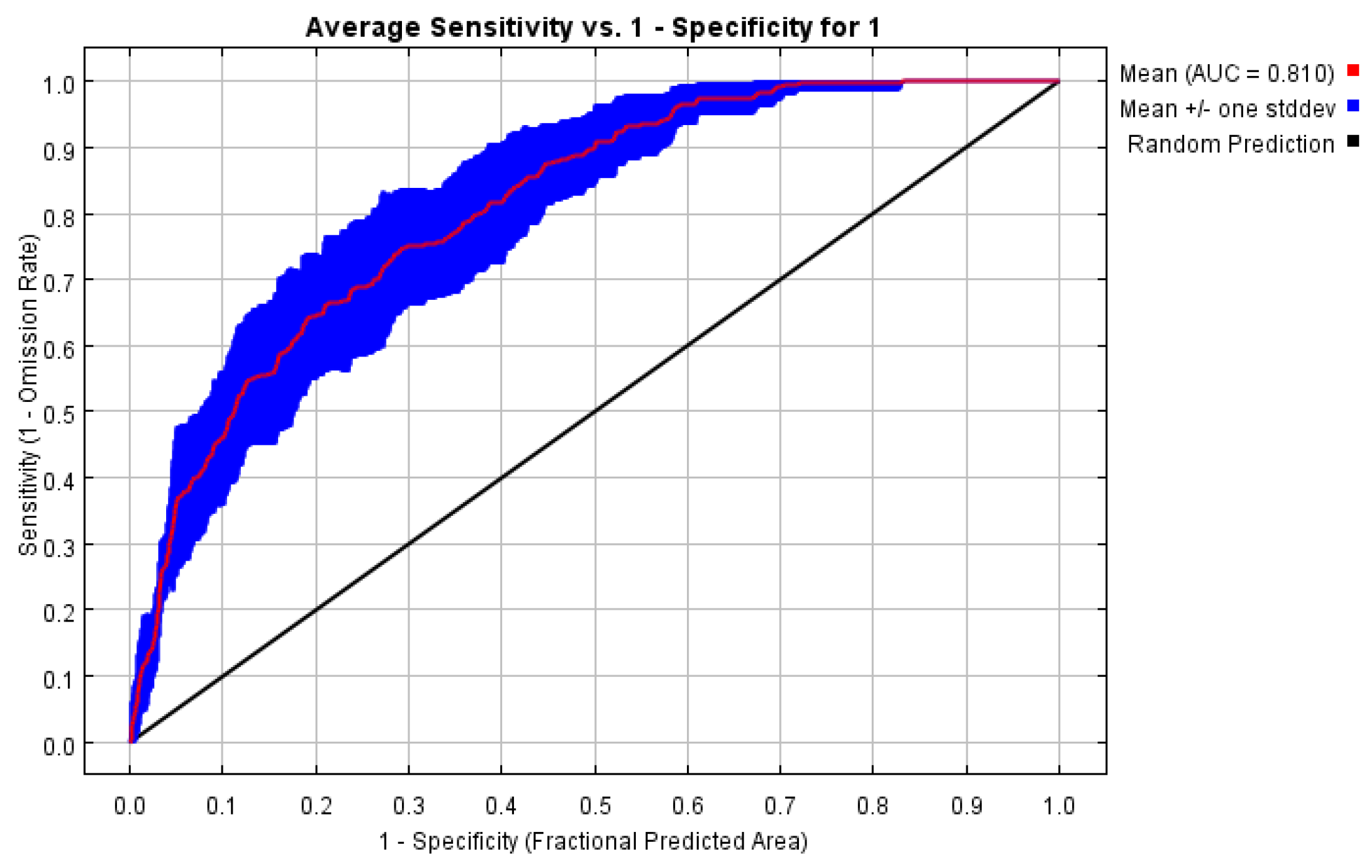
Table 1.
MaxEnt and Ensemble Model Bidirectional Maps.
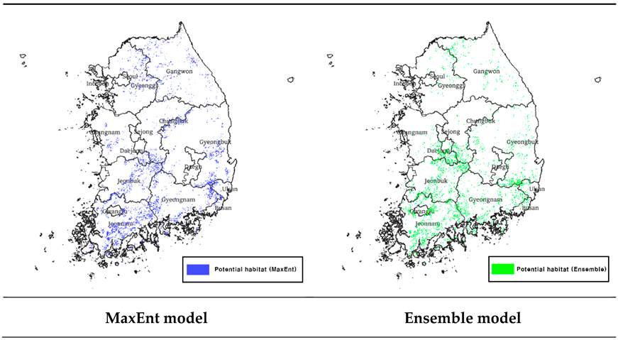
Table 2.
MaxEnt and Ensemble Model Potential Habitat Key Predicted Regions.
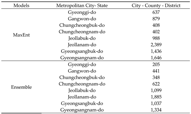
Table 3.
Variable-specific response curves.
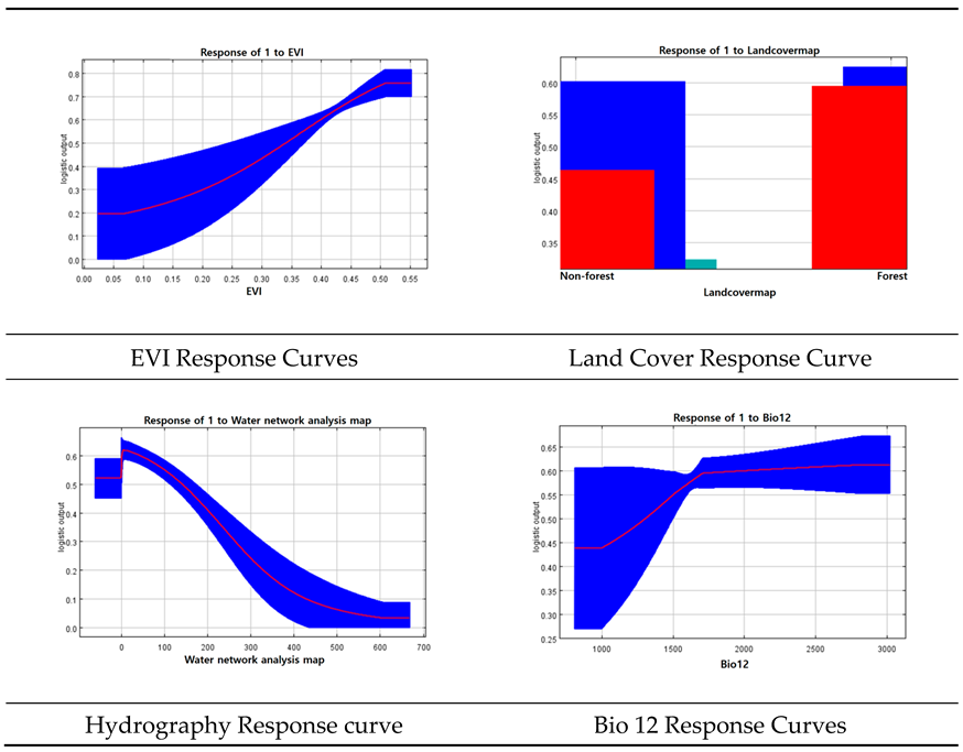
Table 4.
Ensemble model sensitivity, specificity, and accuracy validation results.
| Separation | Sensitivity | Specificity | Accuracy |
|---|---|---|---|
| Kappa | 76.316 | 96.196 | 0.741 |
| TSS | 89.474 | 91.304 | 0.808 |
| AUC | 89.474 | 91.304 | 0.961 |
Table 5.
MaxEnt and Ensemble Model Predicted Potential Habitat Key Overlap Ranges within EVI Ranges.
Table 5.
MaxEnt and Ensemble Model Predicted Potential Habitat Key Overlap Ranges within EVI Ranges.
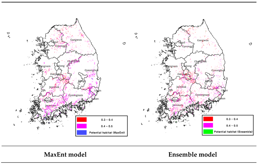
Table 6.
MaxEnt and the ensemble model predicted the potential habitat area by EVI range.
| Separation | Range | Predicted area of potential habitat (㎢) |
|---|---|---|
| MaxEnt | ≤ 0.1 | 0 |
| 0.1 ~ 0.2 | 0 | |
| 0.2 ~ 0.3 | 38 | |
| 0.3 ~ 0.4 | 2,468 | |
| 0.4 ~ 0.5 | 6,225 | |
| 0.5 ~ 0.6 | 51 | |
| 0.6 < | 3 | |
| Ensemble | ≤ 0.1 | 0 |
| 0.1 ~ 0.2 | 7 | |
| 0.2 ~ 0.3 | 84 | |
| 0.3 ~ 0.4 | 3,048 | |
| 0.4 ~ 0.5 | 3,819 | |
| 0.5 ~ 0.6 | 13 | |
| 0.6 < | 0 |
Table 7.
MaxEnt and ensemble model predictions of potential habitat within the scope of the hydrographic map Key overlap areas.
Table 7.
MaxEnt and ensemble model predictions of potential habitat within the scope of the hydrographic map Key overlap areas.
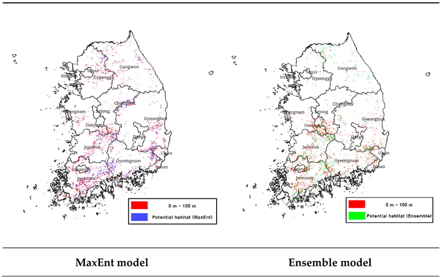
Table 8.
MaxEnt and the ensemble model predicted the potential habitat area by the hydrologic network analysis map extent.
Table 8.
MaxEnt and the ensemble model predicted the potential habitat area by the hydrologic network analysis map extent.
| Separation | Range | Predicted area of potential habitat (㎢) |
|---|---|---|
| MaxEnt | ≤ 100 | 5,592 |
| 101 - 200 | 2,183 | |
| 201 - 300 | 684 | |
| 301 - 400 | 285 | |
| 401 - 500 | 34 | |
| 501 - 600 | 4 | |
| 600 < | 3 | |
| Ensemble | ≤ 100 | 5,404 |
| 101 - 200 | 1,057 | |
| 201 - 300 | 327 | |
| 301 - 400 | 163 | |
| 401 - 500 | 20 | |
| 501 - 600 | 0 | |
| 600 < | 0 |
Table 9.
MaxEnt and Ensemble Model Predicted Potential Habitat Key Overlap Ranges within Bio12 Ranges.
Table 9.
MaxEnt and Ensemble Model Predicted Potential Habitat Key Overlap Ranges within Bio12 Ranges.
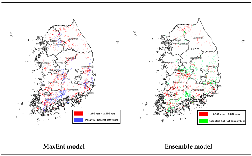
Table 10.
MaxEnt and the ensemble model predicted the potential habitat area by the Bio12 range.
| Separation | Range | Predicted area of potential habitat (㎢) |
|---|---|---|
| MaxEnt | ≤ 500 | 0 |
| 500 – 1,000 | 0 | |
| 1,000 – 1,500 | 668 | |
| 1,500 – 2,000 | 5,768 | |
| 2,000 – 2,500 | 2,266 | |
| 2,500 – 3,000 | 62 | |
| 3,000 – 3,500 | 15 | |
| 3,500 < | 6 | |
| Ensemble | ≤ 500 | 0 |
| 500 – 1,000 | 0 | |
| 1,000 – 1,500 | 1,234 | |
| 1,500 – 2,000 | 4,394 | |
| 2,000 – 2,500 | 1,313 | |
| 2,500 – 3,000 | 25 | |
| 3,000 – 3,500 | 5 | |
| 3,500 < | 0 |
Disclaimer/Publisher’s Note: The statements, opinions and data contained in all publications are solely those of the individual author(s) and contributor(s) and not of MDPI and/or the editor(s). MDPI and/or the editor(s) disclaim responsibility for any injury to people or property resulting from any ideas, methods, instructions or products referred to in the content. |
© 2025 by the authors. Licensee MDPI, Basel, Switzerland. This article is an open access article distributed under the terms and conditions of the Creative Commons Attribution (CC BY) license (http://creativecommons.org/licenses/by/4.0/).
Copyright: This open access article is published under a Creative Commons CC BY 4.0 license, which permit the free download, distribution, and reuse, provided that the author and preprint are cited in any reuse.


