Submitted:
16 June 2025
Posted:
19 June 2025
You are already at the latest version
Abstract
Column tracer experiments reported in the literature have suggested the occurrence of solute accumulation at the interface between different porous materials. This unexpected effect cannot be explained by standard modeling approaches based on Fickian flux continuity and the advection-dispersion equation. In this article, to further analyze this phenomenon, we present reactive transport experiments in a 2D intermediate-scale horizontal tank aimed at visualizing and evaluating the spatiotemporal evolution of a solute plume crossing a sharp interface between coarse and fine material. The solute plume results from the reaction of two fluid solutions that enter the tank in parallel through the tank inlet ports. The reaction product is analyzed through mixing and reaction metrics. Results show that the reaction product also encounters anomalous resistance when crossing the interface between coarse and fine material. This effect is much less pronounced in the fine-to-coarse (FC) transition when the direction of flow is reversed. However, contrary to the reported one-dimensional results (column experiments), this asymmetric anomalous resistance to crossing the interface does not produce solute accumulation behind the interface. Instead, results show an unexpected significant enhancement of the transverse spread of the reaction product in the coarse-to-fine transition (CF) with a slow release in the fine material. As a result, a sudden decrease in the longitudinal resident concentration profile across the heterogeneity interface is observed. Corresponding mixing metrics show that as the apparent transverse dispersivity increases when approaching the interface in the CF transition, the scalar dissipation rate and the total mass reacted also increase, indicating that the CF configuration tends to promote greater solute reactivity near the interface than the FC configuration.
Keywords:
mixing
; solute transport
; sharp soil interfaces
; reactive transport
1. Introduction
Groundwater remediation has become a critical global concern due to the persistent challenge of aquifer pollution and the growing demand for clean water resources [1,2]. Understanding how contaminants are transported, mixed, and react is essential for the successful remediation of polluted aquifers [3,4]. Among various remediation methods, in situ treatment technologies have attracted significant attention in recent years [5,6] because they offer cost-effective and minimally invasive solutions [7]. In this context, the effective mixing of two solutes is crucial to enhancing the performance of in situ treatments [8,9]. Since mixing governs the interaction between the injected remediation fluids and the contaminated groundwater, improved mixing facilitates mass transfer, accelerates chemical reactions, and ultimately leads to a more efficient remediation process [10,11,12]. However, mixing is frequently hindered in porous media by the inherent structural complexities of natural geological formations, which can result in unexpected behavior [13,14,15]. Sharp soil interfaces constitute an important building block of a wide variety of heterogeneous geological systems, representing abrupt transitions between materials with differing permeability and grain size.[16,17,18]. These interfaces, commonly found at sedimentary layer boundaries, fractured rock formations, and engineered remediation barriers [19,20,21], play a pivotal role in controlling transport and mixing. Advancing a quantitative and comprehensive understanding of plume-interface mixing processes is crucial for optimizing remediation strategies, ensuring that injected agents can effectively interact with contaminants [22,23,24], and for refining predictive models of contaminant transport in subsurface systems [12,25,26].
Research over the past decades has demonstrated that sharp interfaces significantly alter solute transport dynamics [17,27,28]. One of the first experimental works on this topic, conducted by Sternberg [27], revealed that sharp interfaces produce transport behaviors that classical advection-dispersion models cannot accurately represent [29,30,31]. These models assume that dispersion across an interface is a simple weighted average of the properties of both media [32]. However, experimental results show that dispersion adjusts to expected values much faster than predicted, suggesting the presence of an additional mechanism at the interface that accelerates this process [28]. Building upon this, Marseguerra and Zoia [28] investigated solute transport across sharp interfaces between coarse and fine media using the random walk method for particle transport simulations. They observed a discontinuity in concentration profiles when solutes crossed the interface [32,33,34], attributing it to solute accumulation on the coarse side before gradually dispersing into the finer medium. This behavior was further suggested by Berkowitz et al. [17], who, through laboratory column experiments on solute migration in composite porous media, indicated that a conservative tracer moving through a coarse-grained segment encounters resistance when entering a finer medium [35,36]. This results in a "slow release" effect, causing a delayed breakthrough curve and increased dispersion. Similarly, Cortis and Zoia [37] showed that particles crossing an interface between materials with different dispersion properties experience asymmetric random forces. These forces disrupt the symmetry assumed in classical transport models, leading to a delayed and spatially uneven arrival of the solute, which further complicates predictions of solute migration [38].
According to mixing processes, although several studies have focused on understanding the effect of heterogeneity on mixing [39,40,41], few works have specifically addressed the impact of sharp interfaces on the mixing [42]. It is well understood that sharp soil interfaces generate steep transverse concentration gradients [17], which can have significant chemical and biological implications. In such contexts, mixing is most pronounced at the contact zones between regions of differing permeability, where reactions are especially intense along these interfaces [43]. In line with this, Perujo et al. [44] demonstrated that coarse-to-fine transitions facilitate the accumulation and transformation of organic matter at the interface. This transition zone thus becomes a region of enhanced microbial activity, promoting increased biomass growth and organic matter degradation. However, the finer sediments limit biofilm development, which ultimately impacts the efficiency of the overall reaction [45]. Despite these insights, there is still much to understand regarding solute transport behavior and the mixing plume dynamics due to sharp soil interfaces [17,42,46]. Specifically, further investigation is needed to visualize the role of sharp soil interfaces on solute transport, the mixing plume evolution, the impact of interfaces on concentration gradients, as well as their role on mixing efficiency in two and three dimensions. Understanding the role of sharp soil interfaces on solute transport and where mixing is most promoted within each medium will provide valuable information for optimizing remediation strategies and improving our overall understanding of subsurface processes [22,23,24].
As a contribution, this article builds upon the results of a novel laboratory-scale experiment, discussing the impact of sharp soil interfaces in both non-reactive transport and mixing processes. Conservative and reactive transport experiments were conducted in a 2D intermediate-scale horizontal tank composed of a bilayer porous medium with a sharp soil interface. To achieve this, a set of four experiments were conducted, considering four different porous medium configurations (porous media packing)—fine (F), coarse (C), fine-to-coarse (FC), and coarse-to-fine (CF). Conservative tracer tests were conducted to visualize solute pulse evolution and obtain concentration breakthrough curves (BTCs), which characterize non-reactive solute transport behavior. In the reactive experiments, colored products were generated and quantified using pixel-by-pixel calibration, converting light intensities into concentration values. The experimental setup allows to monitor and visualize in real-time the spatiotemporal evolution of the tracer and the mixing plume. In this sense, this work aims to demonstrate that: (i) Transport behavior and mixing processes strongly depend on the flow direction. (ii) The sharp soil interface plays distinct roles in solute transport. (iii) The sharp soil interface influences both solute reactivity and mixing efficiency.
The structure of this article is as follows. The Materials and Methods section describes the experimental setup, the porous medium configurations used, the procedure for the reactive transport experiments and tracer tests, the chemical solutions employed, the image acquisition and processing techniques used to capture the evolution of non-reactive and reactive transport, and the explanation of key variables and metrics used for analysis. The Results and Discussion section presents the main findings, including the analysis and discussion of non-reactive solute transport, the spatiotemporal evolution of the reaction product, longitudinal profiles of the reaction product, and mixing metrics and their corresponding profiles. Finally, the Conclusions section provides a summary of the key insights from the study, emphasizing the impact of sharp soil interfaces in mixing processes and transport behavior.
2. Materials and Method
2.1. Experimental Setup
Experiments were conducted in a transparent intermediate-scale horizontal tank made of plexiglass with dimensions of 26 cm in length (L), 20 cm in width (W), and 2 cm in height (H) (refer to Figure 1a). To provide uniform flow conditions, the tank has eight inlet and outlet ports evenly spaced 2 cm apart. All inlet ports are connected to a high-precision multichannel pump (Ismatec IP-N Digital Peristaltic Pump, 24 channels, Pressure Lever Cartridge; 230 VAC). Inlet ports are divided into two groups by means of two 4-channel flow cells to allow the injection of two different fluids, in parallel, through the inlet face of the tank. Outlet ports are ultimately connected to a single tube that freely discharges into a waste container at atmospheric pressure. The height of this tube provides a fixed constant head boundary condition during the experiments. When required for the conservative tracer test, the outlet tube is connected to an Albillia FL24 fluorimeter (see Figure 1a). A pair of piezometers are installed, one at the inlet and the other at the outlet of the tank to measure the effective hydraulic conductivity of the porous medium. The experiments were carried out in a dark room to prevent interference from external light (Figure 1b). Images were captured during both reactive and conservative tracer tests using a Nikon D7100 camera equipped with a Tamron SP AF 17-50mm F/2.8 XR Di II LD Aspherical (IF) Model A16 lens. Transmitted light was used for both experiments, with an LED light placed underneath the tank. Continuous monitoring was performed throughout the experiment, with a fluorometer recording data every second (BTC) and photographs taken every 30 seconds.
2.2. Porous Media Configurations
The horizontal tank was packed in four different porous medium configurations (refer to Figure 1c): a) fine (F), using 1 mm glass beads; b) coarse (C), using 2 mm glass beads; c) fine-to-coarse (FC), with a vertical sharp interface transitioning from 1 mm to 2 mm glass beads; and d) coarse-to-fine (CF), with a vertical sharp interface transitioning from 2 mm to 1 mm glass beads. In the configurations with the sharp soil interface, the interface was positioned at the midpoint of the tank at cm. This vertical interface was created using a 0.1 mm thick methacrylate bar. During packing, the bar was inserted in the middle of the tank to separately distribute the fine and coarse grains, and was carefully removed before sealing the tank. In each porous medium configuration, the tank was wet packed with deionized water (Milli-Q), ensuring that the tank was always filled with water before adding the glass beads. This step was crucial to maintain saturated conditions and prevent the incorporation of air bubbles into the system.
2.3. Reactive Transport Experiments and Tracer Tests
For each porous medium configuration, the experiment was divided into three stages (Figure 2): a) The injection of a conservative tracer test pulse (Figure 2a). This stage was conducted with the purpose of characterizing non-reactive solute transport. This consisted of measuring concentration breakthrough curves (BTCs) at the tank outlet and recording images that show the spatio-temporal evolution of the pulse. This test involved injecting a fluorescein pulse (0.05 mg/L) at a constant flow rate (Q=7.96 ml/min) for 10 minutes. Following the injection, deionized water was injected for 120 minutes to flush the tracer; b) The injection of six standard solutions with known concentrations of Tiron Molybdate () (Figure 2b). In this stage, six light intensity images of Tiron Molybdate at a constant steady-state concentration were recorded with the purpose of establishing a clear relationship between concentration and color intensity pixel-wise. Each standard solution was sequentially injected into the tank, starting from the lowest concentration (C1) to the highest (C6). Each was injected for 1 hour and 30 minutes before imaging. The tank was flushed with distilled water for another hour and a half between injections; c) The simultaneous injection of Molybdate solution () and Tiron solution () through the two separate groups of inlet ports. This setup allows the chemical solutions to uniformly enter into the porous medium through half of the tank’s inlet area, promoting interaction and mixing in the midsection of the tank (Figure 2c). This stage defines the reactive transport experiment, aimed at investigating the role of the sharp interface on solute transport. The total injected flow rate (Q) was 7.96 ml/min. This total flow was equally distributed between the two 4-channel flow cells (Q/2), with each receiving a flow rate of 3.98 ml/min. At the tank outlet, the constant head imposed was 90 cm above tank elevation. The reactive transport experiment lasted 3 hours to ensure that concentrations reach the steady state solution. To prevent density issues, since both and had higher densities than distilled water, the tank was pre-saturated with a 0.4363 M NaCl solution before conducting the reactive transport experiment.
Transport experiments were conducted under advection dominated flow conditions (the properties of each porous medium configuration are presented in Table 1). The grain Péclet number for each porous medium configuration was calculated using , where, v represents the fluid velocity (calculated from the total inflow rate Q, the cross-sectional area A and the porosity through ), d represents the diameter of the glass beads, and D represents the molecular diffusion coefficient of water. The Reynolds number was calculated using , where is the kinematic viscosity of the fluid. The kinematic viscosity is calculated as , where is the dynamic viscosity and is the fluid density. In our experiment, the dynamic viscosity of water was (estimated for a temperature of 20 °C), and the density of water (measured for water with NaCl), resulting in a kinematic viscosity of . The hydraulic conductivity (K) for each porous medium configuration was obtained through Darcy’s law from the piezometric head difference of the tank (). The porosity () for each porous medium configuration was determined by converting the weight of the glass beads used to fill the tank into volume.
2.4. Chemical Solutions
The reactive transport experiment was conducted using a colorimetric reaction involving two solutions: , containing 0.01 M (mol/L) of sodium molybdate dihydrate (MoNa2O4H2O), and , containing 0.02 M of Tiron (1,2-dihydroxybenzene-3,5-disulfonic acid, Ti-2) (refer to Table 2). This reaction resulted in the formation of Tiron Molybdate ( and ) through the following reaction scheme:
During this process, the colorimetric reaction occurs almost instantaneously, with being the colorimetric species [48] and thereby the only component quantified in the image analysis. The color of varies from yellow to dark red. The preparation of the solutions used in the mixing experiment followed the chemical protocol described by Oates and Harvey [49] and Bertran Oller [42], with slight modifications in this study. To prepare the molybdate solution and the Tiron solution , a buffered solution of succinic acid and NaOH was first prepared to maintain the appropriate pH range for the colorimetric reaction. Since remains stable within a pH range of approximately 6.6–7.5, it was essential to ensure that the pH remained within this range during preparation. Finally, Ti and Mo (O4) were added to their respective buffer solutions to obtain and . To further balance the solutions, NaCl was added to the molybdate solution to compensate for the slightly higher density of the Tiron solution . For the quantification of , a visual calibration was created based on the relationship between the image color intensity and the concentration of the generated product. To achieve this, several standard solutions were prepared by combining different volumes of a 0.05 M Ti stock solution and a 0.025 M molybdate stock solution, both buffered to pH 6.6 with 0.13 M succinate and 0.26 M NaOH (refer to Table 2). In addition to a blank, six standard solutions were prepared with concentrations of 0.0002 M, 0.0011 M, 0.0029 M, 0.0042 M, 0.0059 M, and 0.0090 M (refer to Table 3). These solutions were then used to create a calibration curve, which allowed the interpolation of product values based on the observed color. To perform the conservative tracer test and capture the breakthrough curves for each configuration, a 0.05 mg/L fluorescein solution was used, prepared with distilled water.
2.5. Image Acquisition and Processing
During experiments, the camera continuously captured 24-bit RGB color images to record the spatio-temporal evolution of the solute plume in each porous medium configuration ( or fluorescein). The camera settings were manually adjusted and kept constant throughout the experiment, with a relative aperture of f/2.8, a shutter speed of 1/30 seconds, and an ISO setting of 200. The images were processed using the OpenCV library in Python [50,51], following the methodology proposed by Bertran Oller [42]. The concentration of was determined pixel-by-pixel following the method outlined by Castro-Alcalá et al. [43], where the light intensity of each pixel was correlated with those of the standard solutions. This was done using piecewise linear interpolation, with the known concentrations derived from standard solution images obtained prior to the reactive transport experiment. The processing workflow consisted of the following steps: a) Converting both the experimental images and the standard images obtained from each experiment from the raw format (NEF) to 16-bit TIFF images; b) Cropping the images to focus on the region of interest (ROI) with a resolution of 3975 x 3000 pixels, each measuring 0.0066 mm2; c) Centering all images from the reactive transport experiment and the standard solutions to the same (x, y) coordinates to ensure proper interpolation; d) Subtracting the background (chosen for each porous medium configuration) from all standard and experimental images:
where is the light intensity image of the ith standard solution, and is the light intensity of a blank image obtained under steady-state flow conditions prior to each experiment; e) Channel selection, considering only the green band and for the ith standard and experimental images, respectively. The green channel was chosen because it provided an accurate differentiation of the intensities for each standard solution recorded. e) Calculating the concentrations using a piecewise linear interpolation model that relates the green band intensities from the experiment with those of the standard solutions and their corresponding concentrations . The concentration is calculated as follows:
where lies in the range , and the values for each calibration point represent the green band intensity for each pixel in the ith standard image. The concentration is the known concentration associated with the ith standard solution.
2.6. Key Variables and Metrics for Analysis
To evaluate the results, we will use key variables and metrics that characterize transport behavior and mixing processes within the system. The transverse extent of the product plume () defines the influence of mixing along the transverse direction to mean flow. For each porous medium configuration, the transverse extent was determined by binarizing the steady-state plume image using a concentration threshold of , which was established through visual calibration to accurately define the plume edges. After binarization, the plume extent was quantified by measuring the maximum transverse distance (in the y-direction) for each position along the x-axis. In the binary images, black pixels represented the plume region (above threshold), while white pixels indicated the absence of the solute product. From this, an apparent transverse dispersivity () was calculated using the relationship between the transverse extent of the plume and transverse dispersion reported by De Simoni et al. [52] in homogeneous porous media for the same problem. This can be written as
Two other mixing metrics will be also used to analyze the results. On the one hand, the total mass produced by the reaction, i.e., the total mass of (g), was calculated for each configuration by integrating the concentration (mol/L) of throughout the volume of the domain (V) (see Table 1):
This formulation assumes a uniform porosity across the entire domain. However, in the C–F and F–C configurations, the porous medium is composed of two distinct materials with different porosities. In such cases, using a single porosity value leads to an inaccurate estimation of the total reacted mass. To account for the spatial variation in porosity, the calculation must be adjusted by including the porosity inside the integral. Specifically, the domain is divided into two subdomains: and , corresponding to the coarse and fine materials with porosities and , respectively (see Table 1). The corrected expression for the total mass becomes:
Concentrations in mol/L were converted to g/L using the molecular mass of , 841.37 g/mol, based on g/mol and g/mol. On the other, mixing will also be characterized through the scalar dissipation rate, defined by Le Borgne et al. [40] as
In both cases, the unit volume was defined as the product of the pixel area in the -plane and the tank height W as . In addition, results will analyze the longitudinal distribution of the reaction product, which provides insight about the temporal evolution of the longitudinal front of the product plume. To do this, we will use the vertical average of concentrations along the tank width, defined as
Results will be presented using a dimensionless time expressed as pore volume with respect to half of the volume of the tank (). Let us denote as the volume of the first half of the tank and the remaining volume. In our experiment, A can be one material type and B a different one. The water residence time in and can be estimated as and , respectively. From this, the pore volume is defined as
This way, when the injected water has occupied the first half of the porous medium, and when the injected water has occupied the entire porous medium.
3. Results and Discussion
3.1. Non-reactive Solute Transport
The impact of the sharp soil interface was first evaluated by analyzing the behavior of the breakthrough curves (BTCs) of the conservative solute pulse obtained for each porous medium configuration and its spatiotemporal evolution through a series of images, as shown in Figure 3 and Figure 4. Figure 3(a) presents the BTCs in terms of normalized concentration () and pore volumes . For a closer look at the arrival and tailing, they are also shown on a logarithmic scale in Figure 3(b). The results obtained from the non-reactive transport experiments demonstrate a clear direction-dependent transport behavior, which aligns with previous experimental observations [17,46,53]. The BTCs for the coarse (C) and fine (F) porous media exhibit Fickian-Gaussian behavior, a typical characteristic of homogeneous porous systems. When comparing the BTCs, the coarse medium (C) shows an earlier arrival, a lower peak, and a faster tail exit compared to the fine one (F), in line with theoretical expectations [54]. The BTC of the fine-to-coarse (FC) medium also exhibits Gaussian behavior. In Figure 3(a), it can be observed that both the arrival time and the tailing behavior are similar to those of the coarse medium (C), while the peak value is similar to that of the fine medium (F). This suggests that the fine-to-coarse (FC) porous medium behaves as if it were a single homogeneous porous medium, incorporating characteristics of both media; however, previous experiments have indicated that this behavior may depend on the flow rate [55]. In contrast, the BTC obtained for the coarse-to-fine (CF) medium exhibits an asymmetric, non-Fickian behavior, consistent with the experimental results reported by Berkowitz et al. [17]. It presents an early arrival, a low peak value and a long tail typical of BTCs obtained from porous media with mass transfer processes [56,57].
The impact of the sharp interface on solute transport is clearly observed through the spatiotemporal evolution of the solute pulse. Previous solute transport experiments only captured breakthrough curves (BTC), limiting the ability to fully visualize transport processes at the interface [17,53]. In the present study, three key moments are identified for both the fine-to-coarse (FC) and coarse-to-fine (CF) porous medium configurations: just before the plume front reaches the interface (), when the plume front is at the interface (), and just after the plume tail exits the interface (). In the fine-to-coarse (FC) porous medium configuration, before crossing the interface (Figure 4a), the pulse presents a relatively regular front, with a slight tendency to develop more rapidly on the upper side of the tank. As it passes through the interface (Figure 4b), this tendency becomes more pronounced. When the pulse passes almost through the interface, it begins to resemble its previous shape. After completely crossing the interface (Figure 4c), the pulse does not show significant variation, maintaining a shape similar to what it appeared before crossing the interface. On the other hand, in the coarse-to-fine (CF) porous medium configuration, a slight tendency for the pulse to move faster along the bottom side of the tank is observed before reaching the interface (Figure 4d). Upon reaching the interface (Figure 4e), this tendency becomes more pronounced as the pulse shows a strong inclination to develop along the bottom side of the tank, forming small-scale preferential flow channels, a phenomenon reported in Fine-scale heterogeneity of alluvial aquifers [58,59]. The upper side of the pulse experiences a significant delay, resulting in a pulse that no longer resembles its previous shape after passing through the interface (Figure 4f). The pulse becomes distorted, adopting an asymmetrical sigmoidal form.
The results obtained from the non-reactive transport experiments demonstrate that the sharp interface play a different role in transport behavior. In the fine-to-coarse (FC) porous medium configuration, the breakthrough curve (BTC) display a Gaussian distribution, suggesting that the entire medium behaves as a single, homogeneous porous system. The BTC combines features of both porous materials: the arrival time is similar to that observed in the coarse medium BTC, while the peak concentration closely aligns with the BTC from the fine configuration. Regarding the role of the sharp interface, a smooth transition in transport properties is observed, suggesting that the interface apparently acts as a continuous boundary, allowing solute transport to occur as if through a homogeneous medium. In contrast, in the coarse-to-fine (CF) configuration, the resulting breakthrough curves (BTCs) exhibit strong non-Fickian features which align with previous experimental results obtained by Berkowitz et al. [17], including an apparent double peak and an extended tail, which suggests that the coarse-to-fine (CF) porous medium behaves like a dual-permeability system with the interface limiting the mass transfer [6,38]. Visual analysis of the tracer shows that the sharp interface acts as a hydraulic barrier. When the solute pulse reaches the transition, it appears to collide with a wall, which distorts the flow field as it crosses into the fine porous material. This distortion forces the solute pulse to redistribute through localized preferential flow paths.
3.2. Spatiotemporal Evolution of the Reaction Product
We now examine the spatiotemporal evolution of the reaction product plume through a selected series of three images for each porous medium configuration, capturing different stages: at the interface (), after passing through it (), and upon reaching a steady state (), as shown in Figure 5. Upon comparing all cases, we immediately observe that the morphology of the reaction product plume varies depending on the direction, acquiring different transverse extents based on the grain size, which aligns with previous experimental results [60,61]. In the fine (F) medium, in Figure 5(a) the plume initially exhibits an elliptical shape , elongating and widening at the front as it progresses (Figure 5b). By the third stage (Figure 5c), it adopts a final horn-like form, characterized by concave edges, a narrow initial section, and a wider final shape . In the fine-to-coarse (FC) medium, in Figure 5(d) the plume also begins with an elliptical shape . As it advances into the coarse medium (Figure 5e), it expands transversely, adopting a significantly greater transverse extent than it had in the fine medium. In the final stage (Figure 5f), the plume exhibits a narrow shape in the fine medium, transitioning into a much wider form, ultimately resembling a funnel-like shape . In the coarse (C) medium, the plume initially reaches a much greater width than in the fine medium , associated with increased transverse dispersion (Figure 5g). As it advances, it maintains convex edges and an overall oval shape. In the final stage (Figure 5i), the plume develops a bell-like form, adopting a significantly greater thickness than in the fine-grained medium . In the coarse-to-fine (CF) medium, the plume initially presents a thickness similar to that in the coarse medium but ceases to spread laterally upon entering the fine medium, maintaining a constant thickness. After crossing the interface, it adopts a rectangular form with straight edges , eventually transitioning into a bullet-like shape in the final stage (Figure 5l).
The results indicate that the shape of the reaction product plume is direction-dependent and. Grain size governs dispersion [60,61], which in turn determines the transverse extent of the mixing plume [62,63,64,65]. This implies that in coarse media, the transverse extent is greater than in fine media, as previously reported by Sternberg [27]. Consequently, the sharp interface plays a different role in shaping the morphology of the plume depending on the direction: in the fine-to-coarse (FC) configuration, the interface enhances lateral spreading due to increased dispersion in the coarse region, while in the coarse-to-fine (CF) configuration, it restricts lateral spreading, resulting in a constant uniform plume width.
3.3. Longitudinal Profiles of the Reaction Product
The effect that sharp soil interfaces have on reactive transport and mixing processes can be analyzed in greater detail by examining the temporal evolution of the longitudinal distribution of the reaction product. Figure 6 shows the longitudinal profiles of concentrations for each porous medium configuration at five different times = 0.7, = 1, = 1.5, = 2, y = 2.8, illustrating the temporal evolution of the reaction product front along the tank length. The most notable result is that the reaction product encounters anomalous resistance when crossing the interface between coarse and fine material. This effect is much less pronounced in the fine-to-coarse (FC) configuration when the direction of flow is reversed. To analyze this behavior, we begin with the fine-to-coarse (FC) configuration, as shown in Figure 6(b). Initially, the concentration profiles follow a trend similar to that of the fine medium (, ). However, at , a marked discontinuity appears in the concentration profile. Before reaching the interface, the concentration gradually decreases, but upon arrival at the transition zone, it suddenly drops, followed immediately by a significant jump in concentrations. One possible explanation for this behavior comes from the numerical simulations of Leij et al. [33], who demonstrated that concentration discontinuities can result from the way boundary conditions are defined in systems with differing porous media. In their model, a constant solute concentration is maintained in the fine porous layer—representing a so-called first-type boundary condition, commonly used in solute injection experiments. At the interface between the two media, however, they apply a third-type boundary condition, in which the solute flux is governed by both the flow velocity and the transport properties of the medium. The inconsistency between these boundary conditions at different locations in the system leads to a nonuniform redistribution of the solute near the interface, which may account for the concentration jumps observed in our experimental data. At later times, specifically and , the concentration profiles reach significantly higher values () than those observed in the fine medium at equivalent times, suggesting enhanced mixing upon entering the coarse medium.
In the coarse-to-fine (CF) configuration (Figure 6d), the profiles of the reactive product at times and exhibit behavior similar to that of the coarse medium (C). However, at , a discontinuity in concentration is also observed. Initially, the profile follows a trend consistent with that of the coarse medium, but as it approaches the interface, the concentration drops sharply to very low values—lower than those observed in the fine-to-coarse (FC) configuration. However, contrary to previously reported one-dimensional results [17,28,37], this asymmetric anomalous resistance to crossing the interface does not produce solute accumulation behind the interface in the coarse to fine (CF) configuration. After the initial drop, the concentrations begin to increase again, but in a gradual manner, rather than the abrupt jump observed in the FC case. For times and , the sharp drop in concentration remains evident and can also be observed in the longitudinal profiles. Following this, the concentrations gradually recover and eventually reach similar trend to those observed in the coarse medium.
3.4. Mixing Metrics and Profiles of the Reaction Product
To further investigate the impact of the sharp soil interface on the reactive product concentration, we jointly analyze the transverse extent of mixing (), the apparent transverse dispersivity (), and the longitudinal concentration profile (). These metrics allow us to characterize the behavior of the solute plume as it crosses the interface under each porous medium configuration. Our results shows an unexpected significant enhancement of the transverse spread of the reaction product in the coarse-to-fine (CF) configuration with a slow release in the fine material —an effect that is not observed in the fine-to-coarse (FC) configuration and cannot be explained by standard modeling approaches based on Fickian flux continuity and the advection-dispersion equation. We summarize the evidence supporting this behavior below.
- In the coarse-to-fine (CF) porous medium configuration, the transverse extent () initially follows a similar trend to that of the coarse medium () (Figure 7a); however, it surprisingly increases just before reaching the interface (), indicating an unexpected greater transverse dispersion of the plume. After crossing the interface, the transverse extent () stabilizes () and remains constant until the end of the tank. Similarly, the apparent transverse dispersivity () starts with values similar to those obtained in the coarse (C) porous medium () (Figure 7b), but as the interface is approaching, the value significantly increases to about . Beyond this point, the apparent transverse dispersivity () decreases linearly, finishing at roughly . Regarding the longitudinal concentration profile (), a clear discontinuity is observed, reaching its minimum value at the sharp interface (); see Figure 7(c). Afterward, the concentration begins to rapidly rise again, although the values remain significantly lower than those observed in the coarse medium.
- In the fine-to-coarse (FC) configuration, the transverse extent of the reaction product plume () exhibits a dual behavior (Figure 7a), with an inflection point at the interface () where the curve abruptly dips before rising in a sigmoidal manner. From the interface to the end of the tank, the transverse extent () remains significantly larger than in the fine medium, ultimately reaching a final value that exceeds it (). Regarding the transverse dispersivity (), in the first half of the tank, a constant value of is obtained (Figure 7b), which then increases significantly after crossing the interface, reaching final values of . Regarding the longitudinal concentration profile () (Figure 7c) in the fine-to-coarse (FC) media, the curve initially exhibit similar slope that the fine (F) medium. However, upon reaching the interface, the FC curve experiences a slight decline before steepening significantly, leading to notably higher concentration values ()
Although the importance of heterogeneity in controlling solute mixing and reactivity has been widely recognized in previous studies [17,39,40,41,66], no direct studies have specifically analyzed the role of mixing affected by soil interfaces. In this section, we assess the mixing metrics for each scenario by analyzing the mixing efficiency through two key variables: the total reaction product mass of , denoted as (g), and its corresponding scalar dissipation rate , as shown in Figure 8. This analysis is crucial for understanding where mixing is most promoted within a discontinuous heterogeneous porous medium. Upon comparing all cases, we observe different behaviors in the scalar dissipation rate and total mass production near the interface, indicating an asymmetric flow-direction dependence on mixing efficiency and reactivity. To reflect this behavior more clearly, we present below a summary of the evidences.
- In the coarse-to-fine (CF) configuration, the total reaction product mass follows the same trend of the coarse medium up to around = 1.6 (Figure 8a). From this point onward, the total reaction product begins to decline, resulting in lower final values compared to the coarse medium (). Nevertheless, the CF configuration consistently produces a higher total product mass than the FC transition along the entire length of the tank, indicating that even after the decline, mixing and reactivity remain more efficient than in the reverse flow configuration. Regarding the scalar dissipation in the (Figure 8b), the coarse-to-fine (CF) curve reaches a similar final scalar dissipation value as the fine-to-coarse (FC) curve ( () ). However, their temporal evolution is notably different. In particular, the CF configuration consistently exhibits higher values throughout the tank length.
- In the fine-to-coarse (FC) configuration, the total reaction product mass initially follows a pattern similar to that of the fine medium up to approximately (Figure 8a). Beyond this point, the total reaction product mass increases exponentially, eventually surpassing the values observed in the fine medium (). Regarding the scalar dissipation (Figure 8b), the curve exhibits a sigmoidal behavior, similar to the coarse medium. However, after passing through the interface, the slope decreases significantly, eventually reaching much lower values.
Corresponding mixing metrics show that as the apparent transverse dispersivity increases when approaching the interface in the CF transition, the scalar dissipation rate and the total mass reacted also increases, indicating that the CF configuration tends to promote greater solute reactivity near the interface than the FC configuration.
3.5. Conclusions
Sharp soil interfaces formed in porous media between materials with differing grain sizes introduced unexpected effects on solute transport, challenging conventional assumptions about solute transport and reactivity. Understanding their impact on mixing processes and transport behavior is crucial for improving groundwater remediation strategies and predictive models of contaminant migration in subsurface systems. While the impact of sharp soil interfaces had been extensively explored through numerical solute transport models, Darcy-scale experiments designed to visually assess the mechanisms governing their impact on transport behavior and mixing remained largely unknown. To address this gap, we presented well-controlled laboratory experiments conducted in an intermediate-scale horizontal tank simulating sharp transitions between fine and coarse porous materials. The experimental setup allowed for the real-time monitoring and visualization of the spatiotemporal evolution of solute plumes. Finally, we conclude that:
- The sharp soil interface play a different role in transport behavior. In the coarse-to-fine (CF) porous medium, the sharp interface acts as a hydraulic barrier, distorting the flow as it crosses into the fine material, forcing solute redistribution through small-scale preferential flow paths. This leads to an apparently dual-permeability system, with a breakthrough curve (BTC) displaying non-Fickian features, including early arrival, a low peak value, and a long tail. In contrast, the fine-to-coarse (FC) configuration shows a smooth transition of transport properties, behaving apparently as a single homogeneous medium, with a BTC that follows a Gaussian distribution and integrates characteristics of both porous materials.
- Reaction product encounters anomalous resistance when crossing the interface between coarse and fine material. This effect is much less pronounced in the fine-to-coarse (FC) transition when the direction of flow is reversed. However, contrary to the reported one-dimensional results (column experiments), this asymmetric anomalous resistance to cross the interface does not produce solute accumulation behind the interface. Instead, results show an unexpected significant enhancement of the transverse spread of the reaction product in the coarse-to-fine transition (CF) with a slow release in the fine material. As a result, a sudden decrease in the longitudinal resident concentration profile across the heterogeneity interface is observed. Corresponding mixing metrics show that as the apparent transverse dispersivity increases when approaching the interface in the CF transition, the scalar dissipation rate and the total mass reacted also increases, indicating that the CF configuration tends to promote greater solute reactivity near the interface than the FC configuration.
Author Contributions
G.G.-S.: conceptualization, formal analysis, investigation, methodology, software, validation, visualization, and writing—original draft preparation; O.B.: conceptualization, investigation, methodology, and visualization; D.F.-G.: conceptualization, formal analysis, methodology, resources, supervision, and writing—review & editing. All authors have read and agreed to the published version of the manuscript.
Funding
This research was funded by the Ministry of Economic Affairs and Digital Transformation of the Government of Spain (GRADIENT, PID2021-127911OB-I00), the State Agency for Research (AGAUR-SGR-609) of the Generalitat de Catalunya, and the International Doctoral Scholarship Program of Chile, managed by ANID (National Research and Development Agency).
Data Availability Statement
Data will be available upon request to the authors for collaborative research projects.
Acknowledgments
The authors thank Daniela Reales Nuñez of the Universitat Politècnica de Catalunya for her invaluable support during the laboratory work.
Conflicts of Interest
The authors declare no conflicts of interest.
References
- Pous, N.; Balaguer, M.D.; Colprim, J.; Puig, S. Opportunities for groundwater microbial electro-remediation. Microbial biotechnology 2018, 11, 119–135. [Google Scholar] [CrossRef] [PubMed]
- Ravindiran, G.; Rajamanickam, S.; Sivarethinamohan, S.; Karupaiya Sathaiah, B.; Ravindran, G.; Muniasamy, S.K.; Hayder, G. A review of the status, effects, prevention, and remediation of groundwater contamination for sustainable environment. Water 2023, 15, 3662. [Google Scholar] [CrossRef]
- Sathe, S.S.; Mahanta, C. Groundwater flow and arsenic contamination transport modeling for a multi aquifer terrain: Assessment and mitigation strategies. Journal of Environmental Management 2019, 231, 166–181. [Google Scholar] [CrossRef]
- Guo, Z.; Ma, R.; Zhang, Y.; Zheng, C. Contaminant transport in heterogeneous aquifers: A critical review of mechanisms and numerical methods of non-Fickian dispersion. Science China Earth Sciences 2021, 64, 1224–1241. [Google Scholar] [CrossRef]
- Niu, J.; Zhu, X.G.; Parry, M.A.; Kang, S.; Du, T.; Tong, L.; Ding, R. Environmental burdens of groundwater extraction for irrigation over an inland river basin in Northwest China. Journal of Cleaner Production 2019, 222, 182–192. [Google Scholar] [CrossRef]
- Zhang, Y.; Zhu, C.; Bao, C.; Huang, Y.; Jin, Y.; Wu, W.; Wu, D. Modeling of transport and retention of binary particles in porous media with consideration of pore scale effects. Journal of Contaminant Hydrology 2019, 223, 103482. [Google Scholar]
- Kuppusamy, S.; Palanisami, T.; Megharaj, M.; Venkateswarlu, K.; Naidu, R. In-situ remediation approaches for the management of contaminated sites: a comprehensive overview. Reviews of Environmental Contamination and Toxicology 2016, 236, 1–115. [Google Scholar]
- Rolle, M.; Le Borgne, T. Mixing and reactive fronts in the subsurface. Reviews in Mineralogy and Geochemistry 2019, 85, 111–142. [Google Scholar] [CrossRef]
- Ye, Y.; Zhang, Y.; Lu, C.; Xie, Y.; Luo, J. Effective Chemical Delivery Through Multi-Screen Wells to Enhance Mixing and Reaction of Solute Plumes in Porous Media. Water Resources Research 2021, 57, e2020WR028551. [Google Scholar] [CrossRef]
- Piscopo, A.N.; Neupauer, R.M.; Mays, D.C. Engineered injection and extraction to enhance reaction for improved in situ remediation. Water Resources Research 2013, 49, 3618–3625. [Google Scholar] [CrossRef]
- Neupauer, R.M.; Meiss, J.D.; Mays, D.C. Chaotic advection and reaction during engineered injection and extraction in heterogeneous porous media. Water Resources Research 2014, 50, 1433–1447. [Google Scholar] [CrossRef]
- Bertran, O.; Fernàndez-Garcia, D.; Sole-Mari, G.; Rodríguez-Escales, P. Enhancing Mixing During Groundwater Remediation via Engineered Injection-Extraction: The Issue of Connectivity. Water Resources Research 2023, 59, e2023WR034934. [Google Scholar] [CrossRef]
- Le Borgne, T.; Dentz, M.; Villermaux, E. The lamellar description of mixing in porous media. Journal of Fluid Mechanics 2015, 770, 458–498. [Google Scholar] [CrossRef]
- Agartan, E.; Illangasekare, T.H.; Vargas-Johnson, J.; Cihan, A.; Birkholzer, J. Experimental investigation of assessment of the contribution of heterogeneous semi-confining shale layers on mixing and trapping of dissolved CO2 in deep geologic formations. International Journal of Greenhouse Gas Control 2020, 93, 102888. [Google Scholar] [CrossRef]
- Carr, E.J. New semi-analytical solutions for advection–dispersion equations in multilayer porous media. Transport in Porous Media 2020, 135, 39–58. [Google Scholar] [CrossRef]
- Bear, J.; Shapiro, A.M. On the shape of the non-steady interface intersecting discontinuities in permeability. Advances in water resources 1984, 7, 106–112. [Google Scholar] [CrossRef]
- Berkowitz, B.; Cortis, A.; Dror, I.; Scher, H. Laboratory experiments on dispersive transport across interfaces: The role of flow direction. Water resources research 2009, 45. [Google Scholar] [CrossRef]
- Dou, Z.; Zhang, X.; Wang, J.; Chen, Z.; Wei, Y.; Zhou, Z. Influence of grain size transition on flow and solute transport through 3D layered porous media. Lithosphere 2021, 2021, 7064502. [Google Scholar] [CrossRef]
- Qi, X.; Wang, H.; Pan, X.; Chu, J.; Chiam, K. Prediction of interfaces of geological formations using the multivariate adaptive regression spline method. Underground Space 2021, 6, 252–266. [Google Scholar] [CrossRef]
- Alneasan, M.; Behnia, M.; Bagherpour, R. Analytical investigations of interface crack growth between two dissimilar rock layers under compression and tension. Engineering Geology 2019, 259, 105188. [Google Scholar] [CrossRef]
- Lyu, M.; Ren, B.; Wu, B.; Tong, D.; Ge, S.; Han, S. A parametric 3D geological modeling method considering stratigraphic interface topology optimization and coding expert knowledge. Engineering Geology 2021, 293, 106300. [Google Scholar] [CrossRef]
- Neupauer, R.M.; Sather, L.J.; Mays, D.C.; Crimaldi, J.P.; Roth, E.J. Contributions of pore-scale mixing and mechanical dispersion to reaction during active spreading by radial groundwater flow. Water Resources Research 2020, 56, e2019WR026276. [Google Scholar] [CrossRef]
- Du, Z.; Chen, J.; Ke, S.; Xu, Q.; Wang, Z. Experimental investigations on spreading and displacement of fluid plumes around an injection well in a contaminated aquifer. Journal of Hydrology 2023, 617, 129062. [Google Scholar] [CrossRef]
- Du, Z.; Chen, J.; Yao, W.; Zhou, H.; Wang, Z. The critical mixed transport process in remediation agent radial injection into contaminated aquifer plumes. Journal of Contaminant Hydrology 2024, 261, 104301. [Google Scholar] [CrossRef]
- Valocchi, A.J.; Bolster, D.; Werth, C.J. Mixing-limited reactions in porous media. Transport in Porous Media 2019, 130, 157–182. [Google Scholar] [CrossRef]
- Yuan, L.; Wang, K.; Zhao, Q.; Yang, L.; Wang, G.; Jiang, M.; Li, L. An overview of in situ remediation for groundwater co-contaminated with heavy metals and petroleum hydrocarbons. Journal of Environmental Management 2024, 349, 119342. [Google Scholar] [CrossRef]
- Sternberg, S.P. Dispersion measurements in highly heterogeneous laboratory scale porous media. Transport in Porous Media 2004, 54, 107–124. [Google Scholar] [CrossRef]
- Marseguerra, M.; Zoia, A. Monte Carlo investigation of anomalous transport in presence of a discontinuity and of an advection field. Physica A: Statistical Mechanics and its Applications 2007, 377, 448–464. [Google Scholar] [CrossRef]
- Kuo, R.k.H.; Irwin, N.; Greenkorn, R.; Cushman, J. Experimental investigation of mixing in aperiodic heterogeneous porous media: Comparison with stochastic transport theory. Transport in porous media 1999, 37, 169–182. [Google Scholar] [CrossRef]
- Berentsen, C.; Verlaan, M.; Van Kruijsdijk, C. Upscaling and reversibility of Taylor dispersion in heterogeneous porous media. Physical Review E—Statistical, Nonlinear, and Soft Matter Physics 2005, 71, 046308. [Google Scholar] [CrossRef]
- Carr, E.J. Random walk models of advection-diffusion in layered media. Applied Mathematical Modelling 2025, 141, 115942. [Google Scholar] [CrossRef]
- LaBolle, E.M.; Quastel, J.; Fogg, G.E. Diffusion theory for transport in porous media: Transition-probability densities of diffusion processes corresponding to advection-dispersion equations. Water Resources Research 1998, 34, 1685–1693. [Google Scholar] [CrossRef]
- Leij, F.J.; van Genuchten, M.T.; Dane, J. Mathematical analysis of one-dimensional solute transport in a layered soil profile. Soil Science Society of America Journal 1991, 55, 944–953. [Google Scholar] [CrossRef]
- LaBolle, E.M.; Quastel, J.; Fogg, G.E.; Gravner, J. Diffusion processes in composite porous media and their numerical integration by random walks: Generalized stochastic differential equations with discontinuous coefficients. Water Resources Research 2000, 36, 651–662. [Google Scholar] [CrossRef]
- Zhang, C.; Dehoff, K.; Hess, N.; Oostrom, M.; Wietsma, T.W.; Valocchi, A.J.; Fouke, B.W.; Werth, C.J. Pore-scale study of transverse mixing induced CaCO3 precipitation and permeability reduction in a model subsurface sedimentary system. Environmental science & technology 2010, 44, 7833–7838. [Google Scholar]
- Alvarez-Ramirez, J.; Valdes-Parada, F.; Rodriguez, E.; Dagdug, L.; Inzunza, L. Asymmetric transport of passive tracers across heterogeneous porous media. Physica A: Statistical Mechanics and its Applications 2014, 413, 544–553. [Google Scholar] [CrossRef]
- Cortis, A.; Zoia, A. Model of dispersive transport across sharp interfaces between porous materials. Physical Review E—Statistical, Nonlinear, and Soft Matter Physics 2009, 80, 011122. [Google Scholar] [CrossRef] [PubMed]
- Appuhamillage, T.; Bokil, V.; Thomann, E.; Waymire, E.; Wood, B. Occupation and local times for skew Brownian motion with applications to dispersion across an interface. 2011. [Google Scholar]
- Cirpka, O.A.; Frind, E.O.; Helmig, R. Numerical simulation of biodegradation controlled by transverse mixing. Journal of Contaminant Hydrology 1999, 40, 159–182. [Google Scholar] [CrossRef]
- Le Borgne, T.; Dentz, M.; Bolster, D.; Carrera, J.; De Dreuzy, J.R.; Davy, P. Non-Fickian mixing: Temporal evolution of the scalar dissipation rate in heterogeneous porous media. Advances in Water Resources 2010, 33, 1468–1475. [Google Scholar] [CrossRef]
- Dentz, M.; Le Borgne, T.; Englert, A.; Bijeljic, B. Mixing, spreading and reaction in heterogeneous media: A brief review. Journal of contaminant hydrology 2011, 120, 1–17. [Google Scholar] [CrossRef]
- Bertran Oller, O. On the evaluation of mixing in heterogeneous porous media: from laboratory characterization to the design of engineered chaotic flows for practical application. 2023. [Google Scholar]
- Castro-Alcalá, E.; Fernández-Garcia, D.; Carrera, J.; Bolster, D. Visualization of mixing processes in a heterogeneous sand box aquifer. Environmental science & technology 2012, 46, 3228–3235. [Google Scholar]
- Perujo, N.; Sanchez-Vila, X.; Proia, L.; Romaní, A. Interaction between physical heterogeneity and microbial processes in subsurface sediments: a laboratory-scale column experiment. Environmental Science & Technology 2017, 51, 6110–6119. [Google Scholar]
- Perujo, N.; Romaní, A.; Sanchez-Vila, X. A bilayer coarse-fine infiltration system minimizes bioclogging: the relevance of depth-dynamics. Science of the total environment 2019, 669, 559–569. [Google Scholar] [CrossRef] [PubMed]
- Villarreal, R.G. Laboratory experiments on dispersive transport across interfaces: the role of flow cell edges and corners. Ph.D. Thesis, University of Notre Dame, 2013. [Google Scholar]
- Perkins, T.K.; Johnston, O. A review of diffusion and dispersion in porous media. Society of Petroleum Engineers Journal 1963, 3, 70–84. [Google Scholar] [CrossRef]
- Will III, F.; Yoe, J.H. Colorimetric determination of molybdenum with disodium-1, 2-dihydroxybenzene-3, 5-disulfonate. Analytica Chimica Acta 1953, 8, 546–557. [Google Scholar] [CrossRef]
- Oates, P.M.; Harvey, C.F. A colorimetric reaction to quantify fluid mixing. Experiments in fluids 2006, 41, 673–683. [Google Scholar] [CrossRef]
- Bradski, G.; Kaehler, A. Learning OpenCV: Computer vision with the OpenCV library; O’Reilly Media, Inc., 2008. [Google Scholar]
- Howse, J. OpenCV computer vision with python; Packt Publishing Birmingham: UK, 2013; Volume 27. [Google Scholar]
- De Simoni, M.; Sanchez-Vila, X.; Carrera, J.; Saaltink, M. A mixing ratios-based formulation for multicomponent reactive transport. Water Resources Research 2007, 43. [Google Scholar] [CrossRef]
- Chen, Z.; Ma, X.; Zhan, H.; Dou, Z.; Wang, J.; Zhou, Z.; Peng, C. Experimental investigation of solute transport across transition interface of porous media under reversible flow directions. Ecotoxicology and Environmental Safety 2022, 238, 113566. [Google Scholar] [CrossRef] [PubMed]
- Hu, Q.; Brusseau, M.L. Effect of solute size on transport in structured porous media. Water Resources Research 1995, 31, 1637–1646. [Google Scholar] [CrossRef]
- Giacobbo, F.; Giudici, M.; Da Ros, M. About the dependence of breakthrough curves on flow direction in column experiments of transport across a sharp interface separating different porous materials. Geofluids 2019, 2019, 8348175. [Google Scholar] [CrossRef]
- de Vries, E.T.; Raoof, A.; van Genuchten, M.T. Multiscale modelling of dual-porosity porous media; a computational pore-scale study for flow and solute transport. Advances in water resources 2017, 105, 82–95. [Google Scholar] [CrossRef]
- Li, X.; Wen, Z.; Zhan, H.; Zhu, Q.; Jakada, H. On the Bimodal Radial Solute Transport in Dual-Permeability Porous Media. Water Resources Research 2022, 58, e2022WR032580. [Google Scholar] [CrossRef]
- Baratelli, F.; Giudici, M.; Vassena, C. Single and dual-domain models to evaluate the effects of preferential flow paths in alluvial sediments. Transport in porous media 2011, 87, 465–484. [Google Scholar] [CrossRef]
- Baratelli, F.; Giudici, M.; Parravicini, G. Single-and dual-domain models of solute transport in alluvial sediments: the effects of heterogeneity structure and spatial scale. Transport in porous media 2014, 105, 315–348. [Google Scholar] [CrossRef]
- Eidsath, A.; Carbonell, R.; Whitaker, S.; Herrmann, L. Dispersion in pulsed systems—III: comparison between theory and experiments for packed beds. Chemical Engineering Science 1983, 38, 1803–1816. [Google Scholar] [CrossRef]
- Buyuktas, D.; Wallender, W. Dispersion in spatially periodic porous media. Heat and Mass Transfer 2004, 40, 261–270. [Google Scholar]
- Cirpka, O.A.; Rolle, M.; Chiogna, G.; De Barros, F.P.; Nowak, W. Stochastic evaluation of mixing-controlled steady-state plume lengths in two-dimensional heterogeneous domains. Journal of contaminant hydrology 2012, 138, 22–39. [Google Scholar] [CrossRef]
- Liedl, R.; Valocchi, A.J.; Dietrich, P.; Grathwohl, P. Finiteness of steady state plumes. Water resources research 2005, 41. [Google Scholar] [CrossRef]
- Maier, U.; Grathwohl, P. Numerical experiments and field results on the size of steady state plumes. Journal of contaminant hydrology 2006, 85, 33–52. [Google Scholar] [CrossRef]
- Werth, C.J.; Cirpka, O.A.; Grathwohl, P. Enhanced mixing and reaction through flow focusing in heterogeneous porous media. Water Resources Research 2006, 42. [Google Scholar] [CrossRef]
- Kang, Q.; Chen, L.; Valocchi, A.J.; Viswanathan, H.S. Pore-scale study of dissolution-induced changes in permeability and porosity of porous media. Journal of Hydrology 2014, 517, 1049–1055. [Google Scholar] [CrossRef]
Figure 1.
Panel a): Top view of the experimental setup. Inlet flow lines are shown in blue, outlet flow lines in red, and fluorometer flow lines in violet. A) and B) represent the containers with inflow solutions, C) is the peristaltic pump, D) the 4-channel cells, E) the horizontal two-dimensional tank, F) the fluorometer, and G) the container for collecting outflow solutions. Panel b): Side view of the experimental setup, including H) a Nikon D7100 camera, I) the left piezometer, J) an LED light, and K) the right piezometer. Panel c): Packing configurations used in the reactive mixing experiment—fine, coarse, fine-to-coarse (FC), and coarse-to-fine (CF).
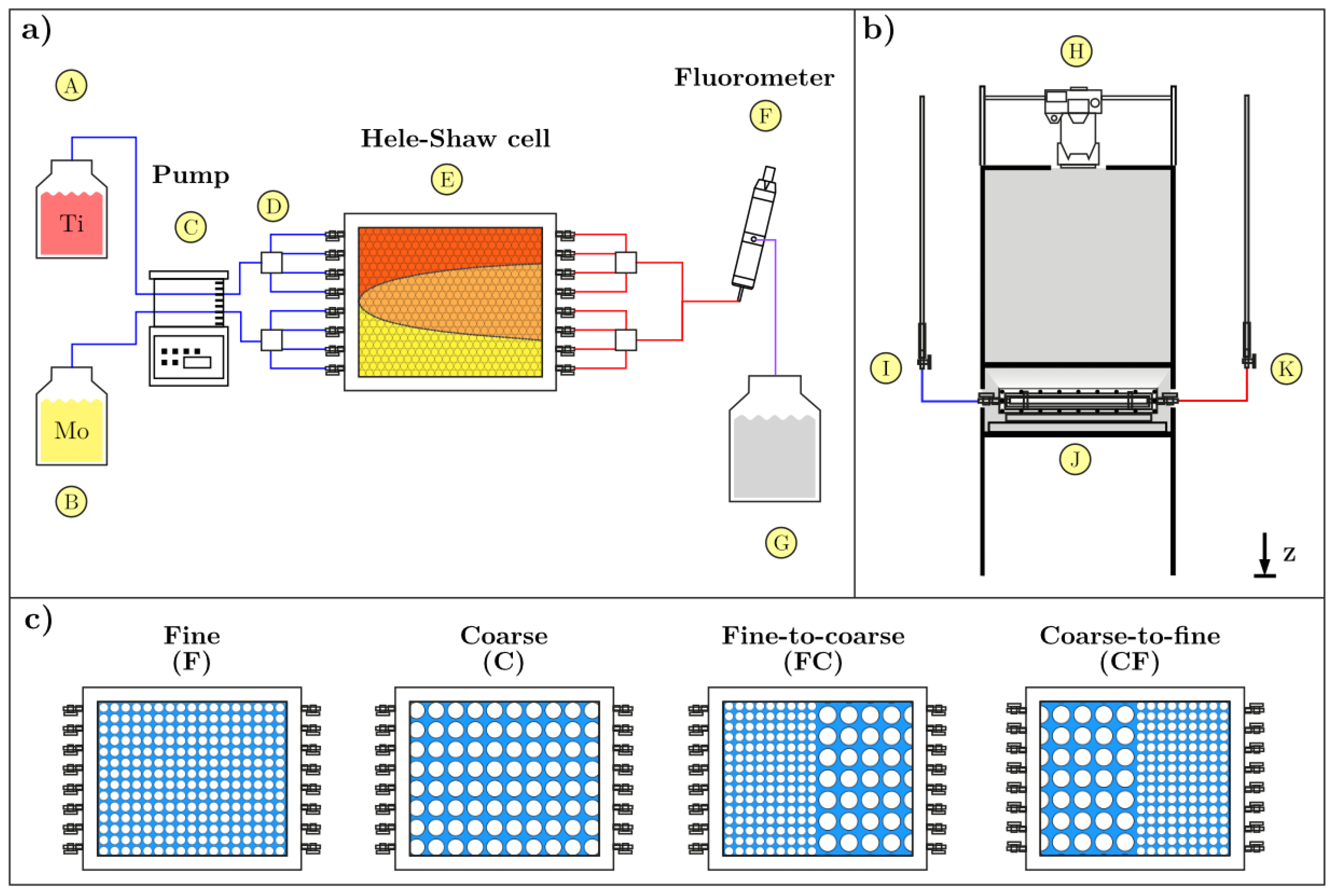
Figure 2.
Detailed procedure conducted for each scenario throughout the experiment. a) Injection of a pulse of a conservative fluorescein tracer () test, b) injection of the six standard solutions used to correlate light intensity with concentration, each followed by a flush with deionized water, c) reactive mixing experiment was conducted using the colorimetric reagents: Tiron (1,2-dihydroxybenzene-3,5-disulfonic acid, Ti–2) and molybdate (sodium molybdate O4). Prior to the experiment, the tank was filled with a NaCl solution.
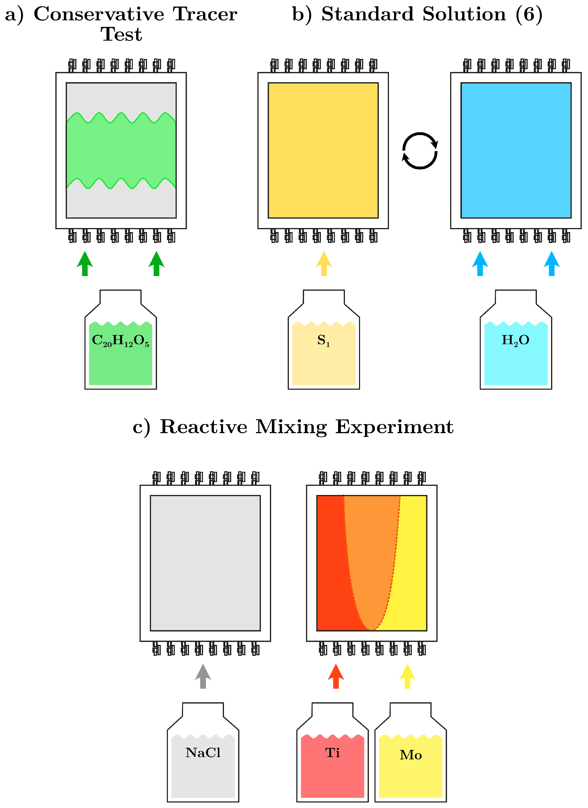
Figure 3.
(a) Breakthrough curves obtained from the fluorescein tracer test considering each scenario. Concentration values are normalized in terms of , and time is expressed in pore volume . (b) Experimental breakthrough curves expressed on a logarithmic scale.
Figure 3.
(a) Breakthrough curves obtained from the fluorescein tracer test considering each scenario. Concentration values are normalized in terms of , and time is expressed in pore volume . (b) Experimental breakthrough curves expressed on a logarithmic scale.
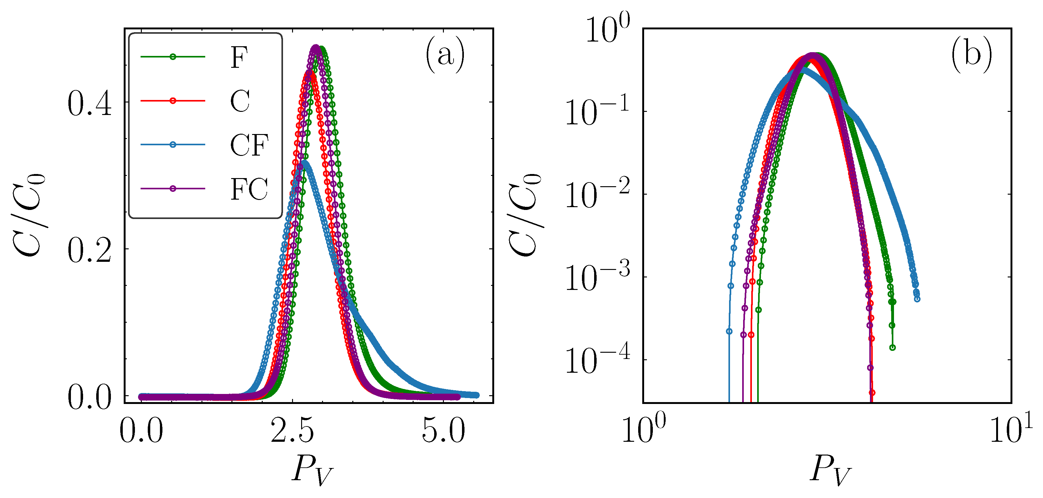
Figure 4.
Spatiotemporal evolution of the fluorescein tracer test pulse considering the fine-to-coarse (FC) scenario in panels (a) to (c) and the coarse-to-fine (CF) scenario in panels (d) to (f). The tank dimensions are shown in terms of length and width in cm, and the tracer concentration is expressed in terms of log(). For each scenario, the evolution is shown at three distinct times: panel (a) and (d) correspond to , just before the tracer reaches the interface; panel (b) and (e) correspond to , after the tracer has crossed the interface; and panel (c) and (f) correspond to , near the end of the tank.
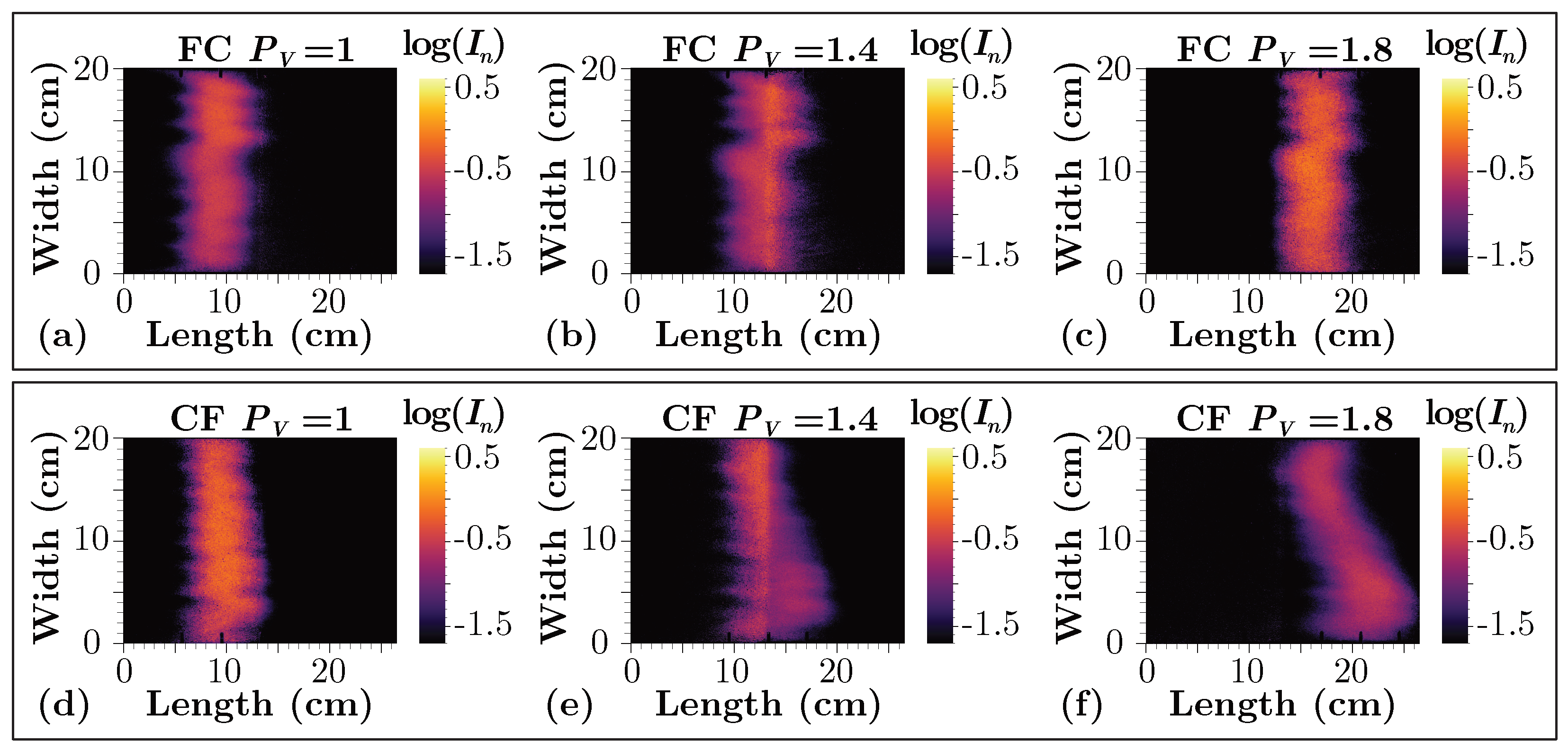
Figure 5.
Spatiotemporal evolution of the mixing plume concentration of (M) in each scenario (F, C, FC, and CF. The image sequence time is expressed in pore volumes, =/ ( parameters are shown in Table 1). Note that is when the plume reaches the sharp soil interface, and is when it reaches the end of the tank. A sequence of three images for each scenario illustrates different stages of the mixing plume evolution: just reaching the interface , nearly reaching the end of the tank , and when it reaches a steady state . Each image shown the dimensions of the experiment in terms of width and length.
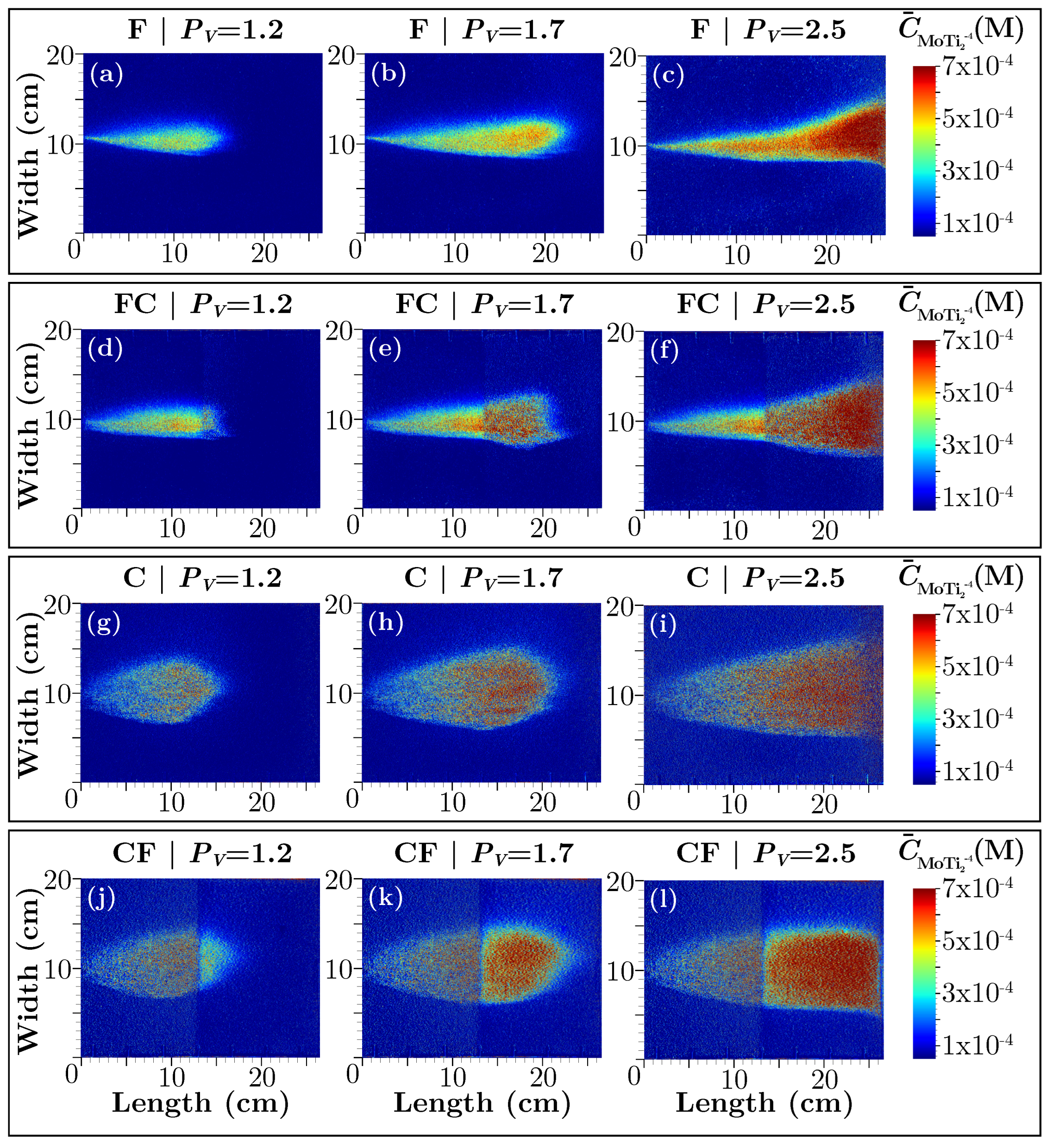
Figure 6.
Longitudinal concentration profiles of calculated for each scenario from the plume image under steady-state conditions, considering five different times: , , , , and . (a) fine (F), (b) fine-to-coarse (FC), (c) coarse (C), and (d) coarse-to-fine (CF).
Figure 6.
Longitudinal concentration profiles of calculated for each scenario from the plume image under steady-state conditions, considering five different times: , , , , and . (a) fine (F), (b) fine-to-coarse (FC), (c) coarse (C), and (d) coarse-to-fine (CF).
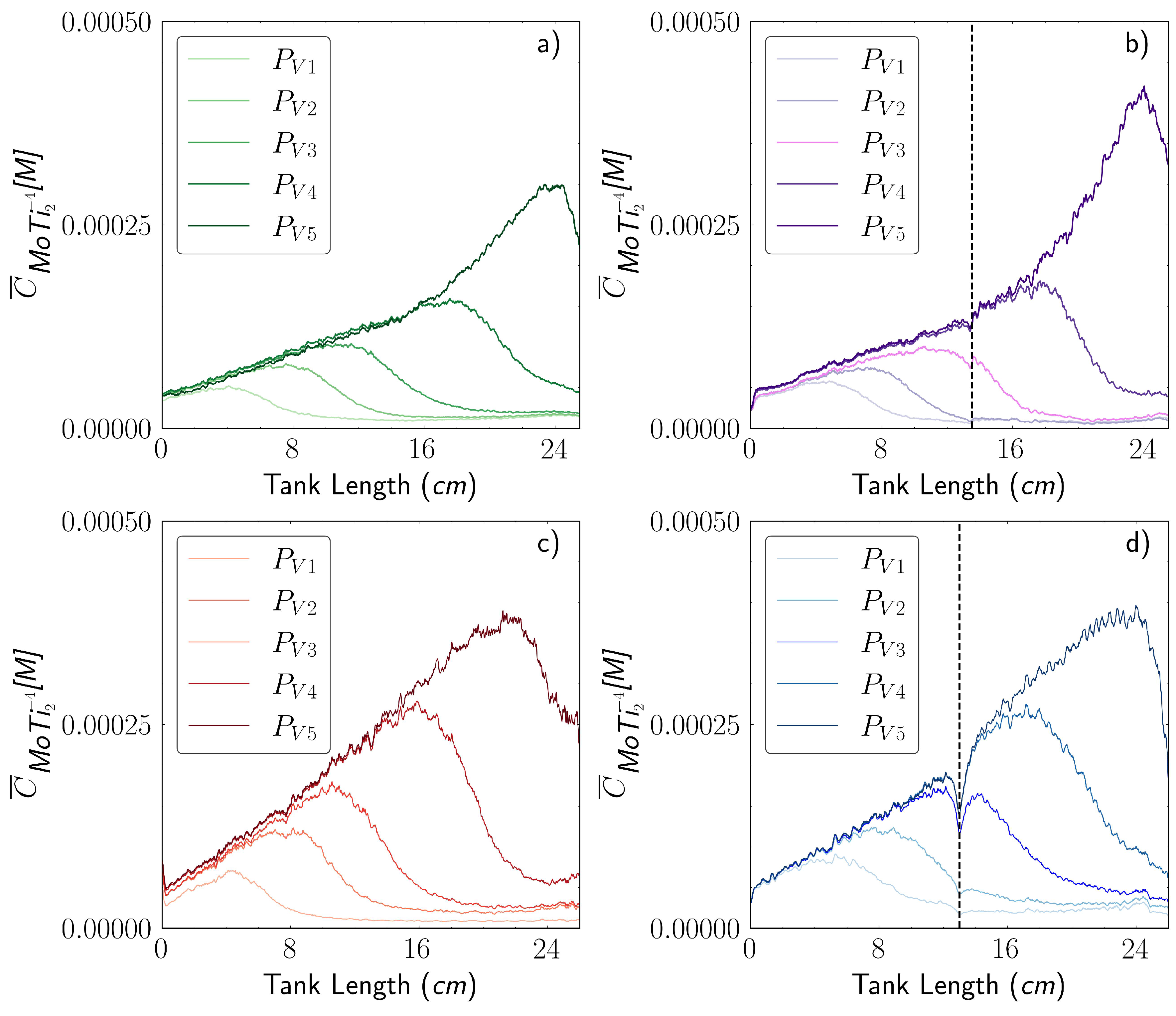
Figure 7.
Panel (a): evolution of transverse plume extent () expressed in cm, calculated for each scenario from the plume image under steady-state conditions. Panel (b): apparent transverse dispersivity () evolution. Panel (c): longitudinal concentration profile of , calculated for each scenario from the plume image under steady-state conditions.
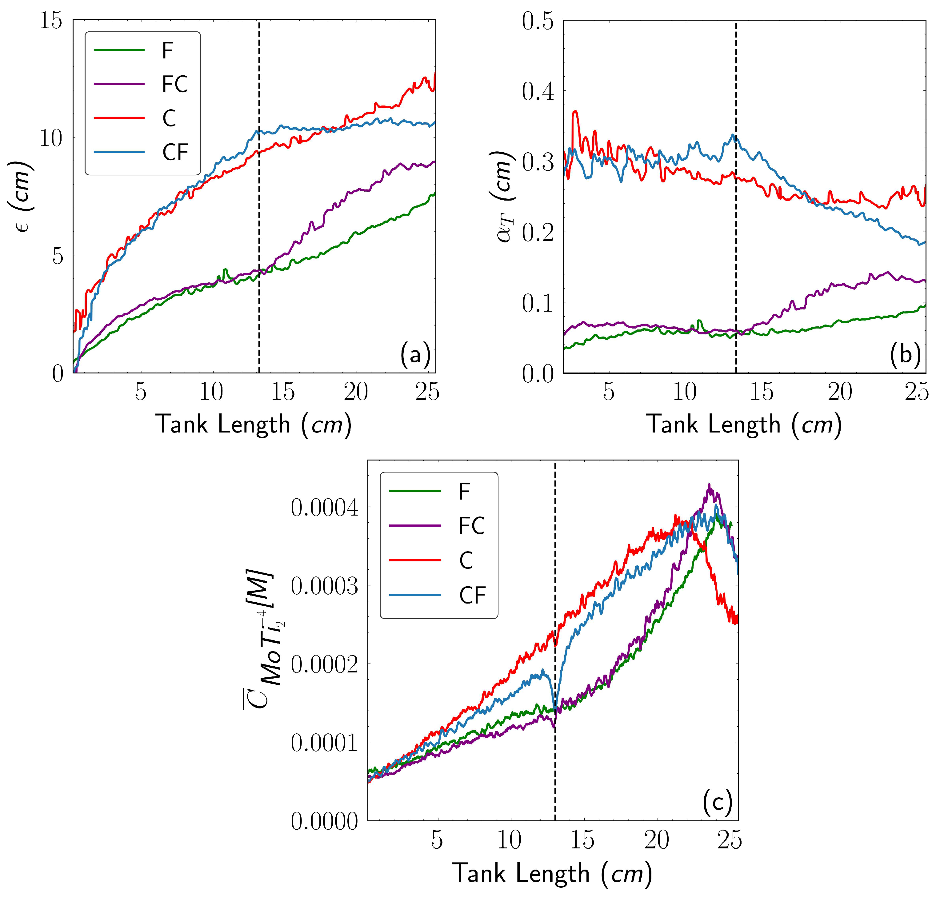
Figure 8.
Panel (a): total mass of (g) as a function of time (); Panel (b): scalar dissipation rate (g) as a function of time (); Panel (c): total mass of with both axes on a logarithmic scale; Panel (d): scalar dissipation rate (g) in log scale as a function of time ().
Figure 8.
Panel (a): total mass of (g) as a function of time (); Panel (b): scalar dissipation rate (g) as a function of time (); Panel (c): total mass of with both axes on a logarithmic scale; Panel (d): scalar dissipation rate (g) in log scale as a function of time ().
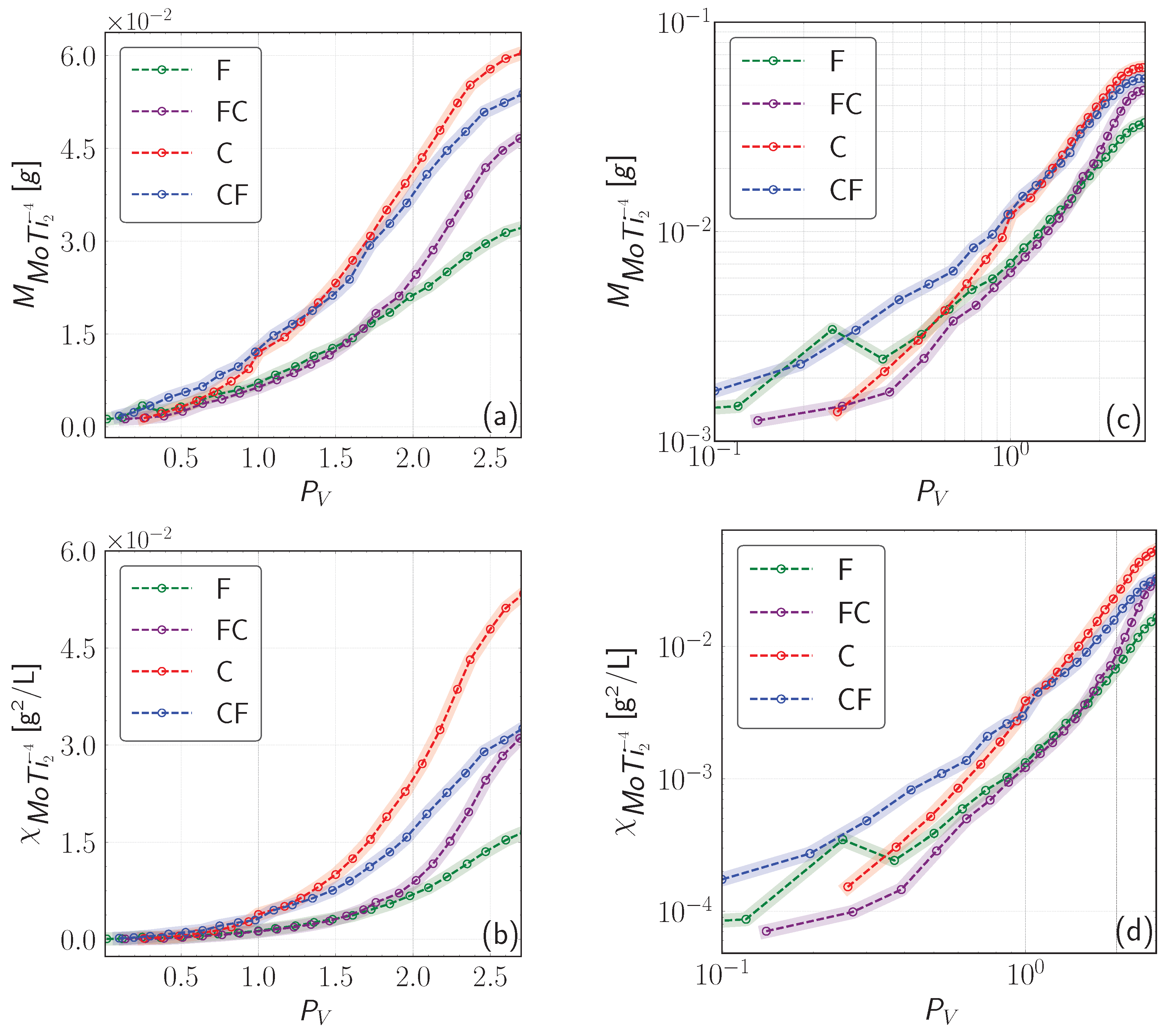

Table 1.
Initial experimental conditions.
| Symbol | Properties | Value | Units |
| Q | Total flow rate | ||
| Fine (F) glass bead size | 1 | mm | |
| Coarse (C) glass bead size | 2 | mm | |
| D | Water molecular diffusion (*) | ||
| Re | Reynolds number (fine) | 1.08 | - |
| Re | Reynolds number (coarse) | 1.98 | - |
| Kinematic viscosity (**) | |||
| Dynamic viscosity | |||
| Density of fluid | |||
| A | Section area | ||
| L | Tank length | m | |
| W | Tank width | m | |
| H | Tank height | m | |
| Porosity (fine) | 0.31 | - | |
| Porosity (coarse) | 0.34 | - | |
| Darcy velocity (fine) | m/s | ||
| Darcy velocity (coarse) | m/s | ||
| Pe | Grain Péclet number (fine) | 106.9 | - |
| Pe | Grain Péclet number (coarse) | 195 | - |
| Height Difference (fine) | 0.025 | m | |
| Hydraulic gradient (fine) | - | ||
| Hydraulic conductivity (fine) | 29.8 | ||
| Height Difference (coarse) | m | ||
| Hydraulic cond. (fine) | - | ||
| Hydraulic cond. (coarse) | 53.22 |
: Information obtained from Perkins and Johnston [47] (*). The dynamic viscosity of pure water was used, as the variation due to solutes in the solution was minimal (**).
Table 2.
Chemical properties of reactive and stock solutions.
| Properties | (Mo) | (Ti) | Stock 1 | Stock 2 |
| O4 | 0.01 M | - | 0.025 M | - |
| Ti | - | 0.02 M | - | 0.05 M |
| Succinic Acid | 0.13 M | 0.13 M | 0.13 M | 0.13 M |
| NaOH | 0.26 M | 0.26 M | 0.26 M | 0.26 M |
| NaCl | 0.0761 M | - | - | - |
| RI (Refraction Index) * | 1.337 | 1.337 | - | - |
| Density (g/) | 1.0136 | 1.0136 | - | - |
: * The measurements were obtained using a refractometer.
Table 3.
Standard solutions.
| Standard solutions | Stock 1 | Stock 2 | (M) |
| 90% | 10% | 0.000244 | |
| 80% | 20% | 0.001123 | |
| 70% | 30% | 0.0029 | |
| 65% | 35% | 0.00423 | |
| 60% | 40% | 0.00586 | |
| 50% | 50% | 0.009 |
Disclaimer/Publisher’s Note: The statements, opinions and data contained in all publications are solely those of the individual author(s) and contributor(s) and not of MDPI and/or the editor(s). MDPI and/or the editor(s) disclaim responsibility for any injury to people or property resulting from any ideas, methods, instructions or products referred to in the content. |
© 2025 by the authors. Licensee MDPI, Basel, Switzerland. This article is an open access article distributed under the terms and conditions of the Creative Commons Attribution (CC BY) license (http://creativecommons.org/licenses/by/4.0/).
Copyright: This open access article is published under a Creative Commons CC BY 4.0 license, which permit the free download, distribution, and reuse, provided that the author and preprint are cited in any reuse.


