Submitted:
16 June 2025
Posted:
17 June 2025
You are already at the latest version
Abstract
The application of artificial intelligence (AI) techniques has improved the accuracy of forest species identification, particularly in timber inventories conducted under Sustainable Forest Management (SFM). This study developed and evaluated machine learning models to recognize 16 Amazonian timber species using digital images of tree bark. Data were collected from three SFM units located in Nova Maringá, Feliz Natal, and Cotriguaçu, in the state of Mato Grosso, Brazil. High-resolution images were processed into sub-images (256 × 256 pixels), and two feature extraction methods were tested: Local Binary Patterns (LBP) and pre-trained Convolutional Neural Networks (ResNet50, VGG16, InceptionV3, MobileNetV2). Four classifiers—Support Vector Machine (SVM), Artificial Neural Networks (ANN), Random Forest (RF), and Linear Discriminant Analysis (LDA)—were used. The best result (95% accuracy) was achieved using ResNet50 with SVM, confirming the effectiveness of transfer learning for species recognition based on bark texture. These findings highlight the potential of AI-based tools to enhance accuracy in forest inventories and support decision-making in tropical forest management.
Keywords:
Forest census
; forest species recognition
; transfer learning
; Amazon flora
1. Introduction
The Amazonian flora comprises approximately 30% of all arboreal individuals in South America and represents one of the world’s leading producers of tropical timber [1,2]. As timber market activity intensifies in the region, it becomes increasingly necessary to regulate resource extraction through Sustainable Forest Management (SFM) practices [3,4]. SFM is defined as the management of forests to generate economic, social, and environmental benefits while preserving ecosystem functions [5]. One of its key requirements is a 100% forest inventory, which entails both quantitative and qualitative data collection, including the botanical identification of tree species [6,7].
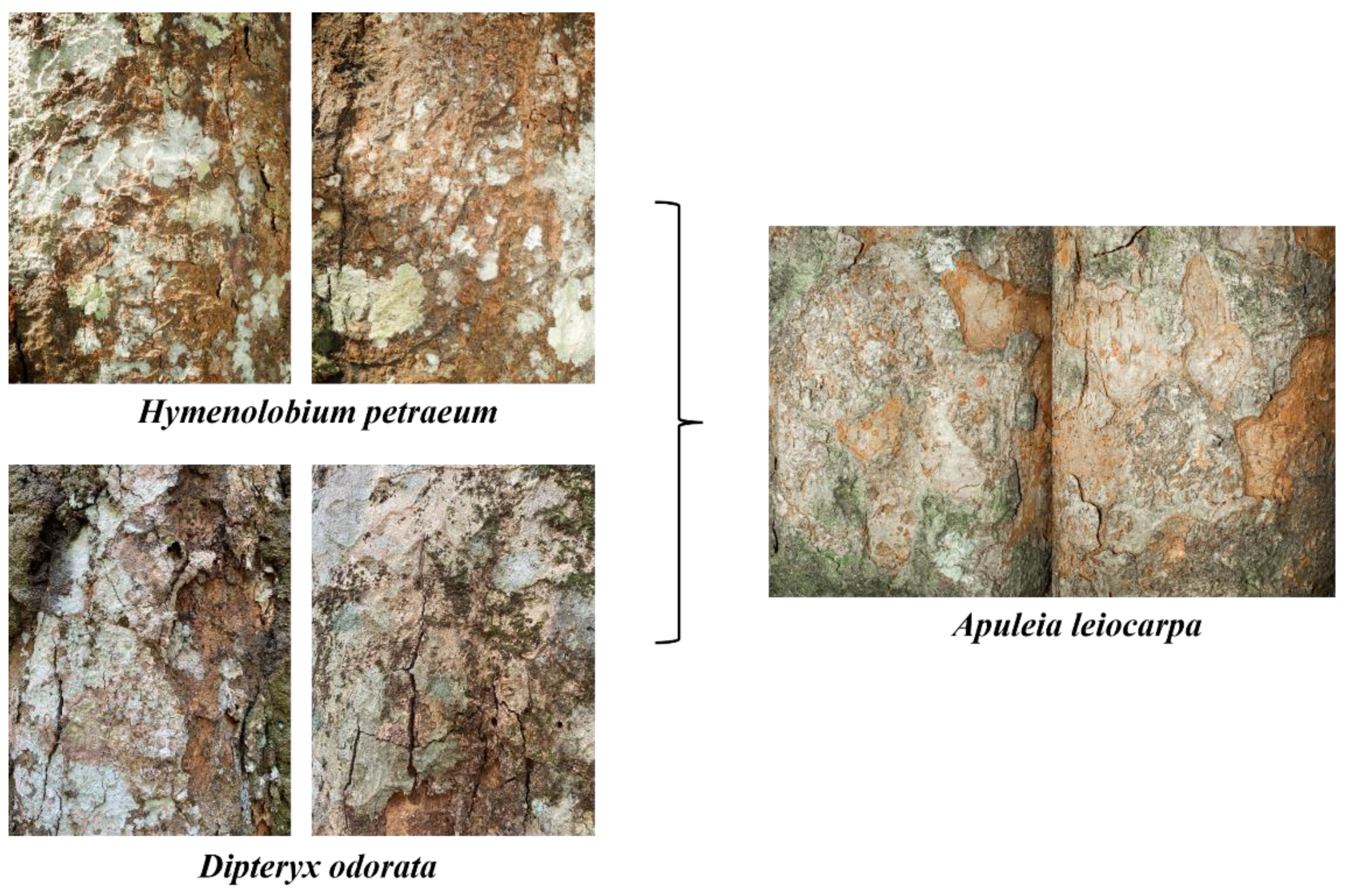
Accurate botanical identification in the Amazon is challenging due to the morphological similarity among species. It traditionally relies on the collection of reproductive material—leaves, flowers, fruits, and seeds—which must be compared with herbarium specimens [8,9]. In timber-focused SFM, however, identification is often performed by local experts known as “mateiros”, who rely on vernacular names and macroscopic traits such as bark color, texture, scent, and the presence or absence of exudates [10,11].
While vernacular identification is valuable, it often leads to errors such as misidentification of endangered species, confusion in trade nomenclature, and inconsistencies when converting common names to scientific ones based on outdated official species lists [12,13,14]. These issues are well documented in studies that report spelling mistakes, inconsistent nomenclature, and incomplete taxonomic identification in Sustainable Forest Management Plans (SFMPs), largely due to dialectal variation and limited oversight [15,16].
To address these challenges, recent studies have explored computer vision and artificial intelligence techniques to support botanical identification [11,17,18]. These methods involve extracting features from digital images of plant organs [19,20,21] and classifying them using machine learning algorithms such as Artificial Neural Networks (ANN) and Support Vector Machines (SVM) [22,23,24]. Although most models rely on leaf or wood images [25,26,27,28], bark images present a more practical alternative in Amazonian forest conditions, where canopy height and phenology often limit the collection of other structures [18,29,30].
Despite the progress in computational models for plant recognition [31,32,33,34,35] there is currently no automated system tailored for identifying the main commercial species of the Amazon during forest inventories. This study aims to fill that gap by developing and evaluating machine learning models based on bark images for the identification of 16 commercially important species. The models incorporate different feature extraction techniques and classification algorithms, contributing to the improvement of species identification processes in timber-focused SFM.
2. Materials and Methods
2.1. Areas of study
This study was conducted in three Sustainable Forest Management (SFM) Demonstration Units (DUs) aimed at commercial timber production, located in the state of Mato Grosso, Brazil: DU1 – Farm Pérola (Nova Maringá), DU2 – Farm Boa Esperança (Feliz Natal), and DU3 – Farm São Nicolau (Cotriguaçu) (Figure 1).
These DUs are situated within regions of the Amazon biome, which occupies approximately 53.5% of Mato Grosso’s territory and overlaps with elements of the Cerrado and Pantanal biomes [36]. The predominant forest types in the study areas include Dense and Open Ombrophilous Forests and Seasonal Forests, characterized by high biodiversity and commercial interest for timber. The regional climate is tropical, with average temperatures ranging from 24.3°C to 25.7°C and annual rainfall between 2,000 and 2,500 mm [37,38].
These areas were selected for their ecological representativeness and economic relevance within legal SFM frameworks in the Amazon. They provide a realistic field context for testing artificial intelligence tools aimed at improving species identification in operational forest inventories.
2.2. Image acquisition
The species were selected based on the list of forest species of most significant commercial interest in the state of Mato Grosso, provided by the Center of Wood Producing and Exporting Industries of Mato Grosso (CWPEIMG), and taking into account the occurrence and abundance of individuals in the collection areas.
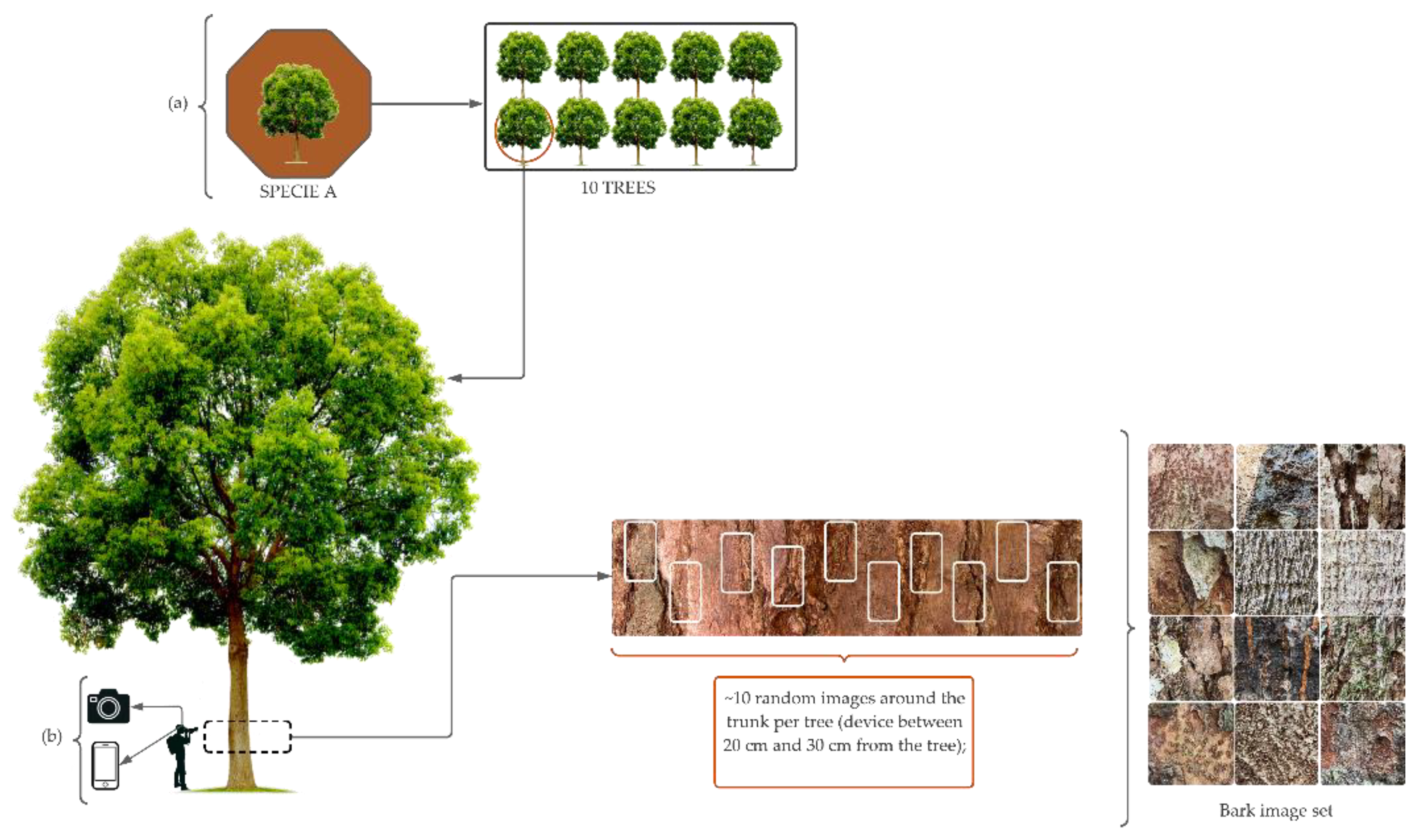
In the field, images were taken of the bark (rhytidome) of 10 trees per species, using two devices: a Canon camera and an iOS iPhone 11 device, obtaining images with resolutions of 3024 x 4032 and 4000 x 5328, respectively (Refer to the Appendix A – Figure A1 for additional details). On the trees, the region in which the images were captured ranged in height from 30 cm to 1.40 m from the ground, and a distance of between 20 cm and 40 cm from the device to the trunk, depending on the conditions found in the field.
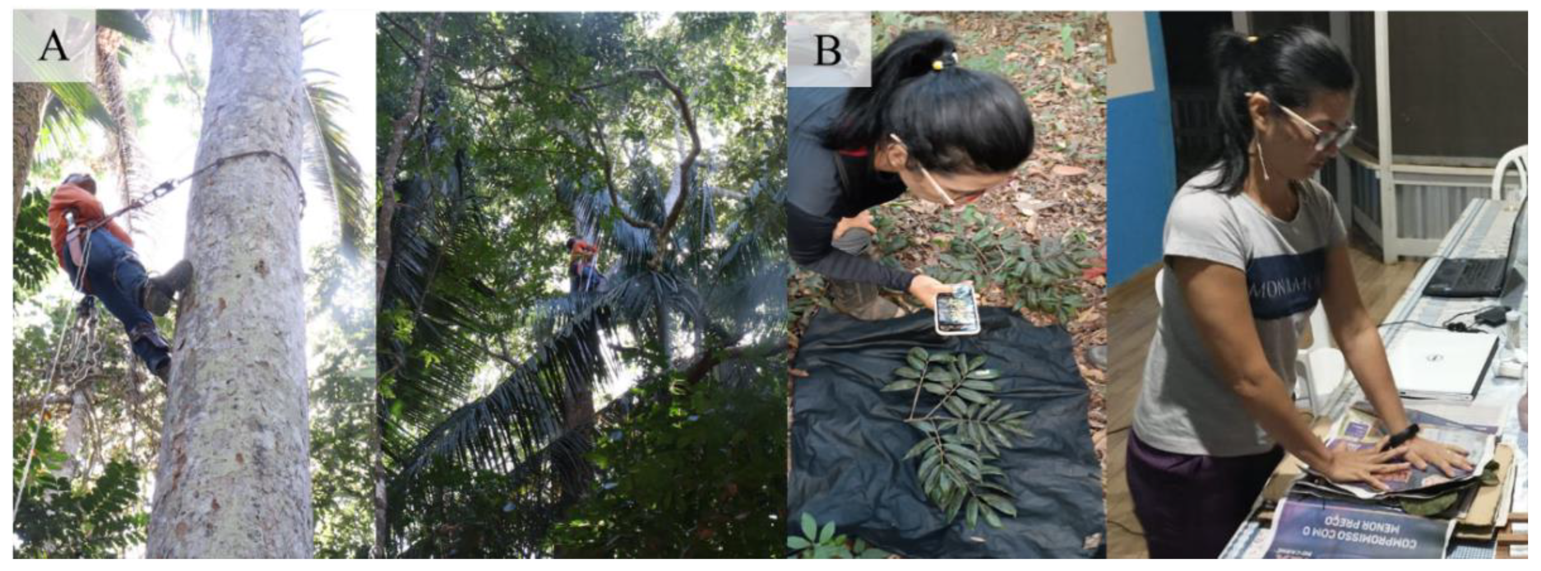
Many factors made it difficult to acquire images, such as low light (or even too much due to direct sunlight on the tree trunk) and the presence of mosses (or lichens) and termites in the bark. Therefore, in areas of the forest with low light levels, a reflector (YN600L II - Pro Led Video Light) was used to improve the light conditions for capturing the image (Refer to the Appendix A – Figure A2 for additional details).). In addition, in trees with a high incidence of mosses, lichens, or termites, we looked for areas of the trunk free of these living beings to highlight the characteristics of the tree bark in the captured image.
The acquired images were carefully evaluated to identify quality problems or undesirable elements that could affect the extraction of features and subsequent learning of the models. The image base consisted of 2,803 bark images belonging to 16 species, 16 genera, and 9 families (Table 1). Figure 2 shows samples of bark images from the 16 tree species.
2.3. Identifying species and collection botanical material
In the field, species identification is a complex task, but one that is fundamental to ensuring the correct labeling of images and constructing a reliable species recognition system. Therefore, species identification was initially carried out by a Parabotanist, who climbed at least five trees per species to collect botanical material, sampling 83 specimens from 16 species.
All the botanical material was pressed, and then exsiccates were mounted to be sent to the Felisberto Camargo Herbarium (HFC) at the Federal Rural University of Amazonia to confirm the identification (Refer to the Appendix A – Figure A3 for additional details).)
2.4. Extraction of sub-images (patches)
To improve feature extraction and optimize computational efficiency, the original high-resolution bark images (3024 × 4032 and 4000 × 5328 pixels) were segmented into smaller sub-images. This patch-based approach enhances the detection of local texture patterns and increases dataset variability, which is particularly beneficial for training convolutional neural networks (CNNs).
Initially, all images were resized to 20% of their original resolution to reduce preprocessing time while preserving relevant visual features. From each resized image, 50 random sub-images (patches) of 256 × 256 pixels were extracted, resulting in a total of 140,150 patches from 2,803 original images. The patch size was chosen to ensure compatibility with standard CNN input dimensions (e.g., ResNet50: 224 × 224; InceptionV3: 299 × 299).
The number of patches per image was defined considering the trade-off between dataset augmentation and computational cost. Previous studies used between 9 and 80 patches per image depending on class diversity and resource availability [29,39]. In this study, 50 patches were considered sufficient to balance performance and processing time across 16 species classes.
2.5. Extracting features from original images and sub-images
The feature extraction process is an essential step in the successful modeling of automatic classifiers [11]. Thus, two strategies for extracting features from digital images of tree bark were evaluated: i) Local Binary Patterns (LBP) and ii) pre-trained Convolutional Neural Networks (CNN) (ResNet50, VGG16, InceptionV3 and MobileNetV2). These features were extracted from original high-resolution images (3024 x 4032 and 4000 x 5328 pixels) captured by two devices (CANON and iOS iPhone 11) and from 256 x 256 pixel sub-images randomly extracted from the original images.
2.5.1. Subsubsection
Local Binary Patterns (LBP) is a robust and efficient texture descriptor, invariant to grayscale variations, originally proposed by [41]. It combines statistical and structural texture analysis by encoding the local neighborhood of each pixel into a binary code that reflects primitive texture patterns such as edges, spots, and corners.
Due to its simplicity, low computational cost, and effectiveness in capturing fine-grained textures, LBP has been widely used in image classification tasks, including bark recognition.
Mathematically, an LBP code for a given pixel is calculated as follows:
where P is the number of circular neighbors, R is the radius, xc is the intensity of the central pixel, and xp are the neighboring pixel values.
To enhance rotation invariance and compactness, the rotation-invariant uniform LBP () proposed by [42] was also used. In this study, RGB images were first converted to grayscale, and six LBP configurations were applied to both the original and patch images:
- Uniform and rotation-invariant: , , ;
- Uniform and non-invariant: , , .
From each configuration, histograms of LBP code occurrences were extracted. To standardize the feature distributions and improve model convergence, Z-score normalization was applied:
2.5.2. Transfer learning
Convolutional Neural Networks (CNNs) are a class of deep learning models characterized by feedforward architectures incorporating convolutional operations and depth [43]. However, training CNNs typically requires large datasets and substantial computational resources. Transfer Learning offers an alternative by adapting pre-trained networks to new but related tasks, thereby leveraging previously acquired knowledge and reducing training demands [23,44].
This study employed four pre-trained CNN architectures—ResNet50, VGG16, InceptionV3, and MobileNetV2—selected based on their proven performance in similar plant classification applications [45,46,47]. ResNet50, a 50-layer residual network, was trained on over one million images from the ImageNet dataset, capable of classifying up to 1000 categories [33]. VGG16 comprises 16 trainable layers and was developed by the Visual Geometry Group at the University of Oxford, widely applied in computer vision [48]. InceptionV3 includes approximately 48 layers, utilizing multiple kernel sizes and pooling methods to optimize computational efficiency [49]. MobileNetV2, with around 53 layers, balances computational cost and accuracy, making it suitable for mobile devices [50].
All networks were initialized with ImageNet weights, and their final classification layers were replaced by a Global Average Pooling (GAP) layer to serve as feature extractors. GAP effectively reduces feature map dimensionality and the number of parameters, minimizing overfitting risk without substantial information loss. Images were pre-processed according to each network’s standards, and the resulting feature vectors were input to subsequent classification algorithms.
2.6. Algorithms, cross-validation and performance metrics
2.6.1. Classification algorithms
Four machine learning algorithms were employed: Support Vector Machine (SVM), Artificial Neural Networks (ANN), Random Forest (RF), and Linear Discriminant Analysis (LDA). SVM is a supervised learning method for classification and regression that maps features into a new space and defines a decision boundary separating classes; multi-class problems are addressed via multiple binary classifiers [51,52,53].
ANNs mimic human brain information processing, providing a framework for regression and classification through adjustable connections and specific architectures [54]. RF is an ensemble technique combining outputs of multiple decision trees for classification and regression [55,56]. LDA is a supervised algorithm used for classification and dimensionality reduction, projecting data into lower-dimensional space by maximizing between-class variance relative to within-class variance [57,58].
2.6.2. Image division and cross-validation
The bark image dataset (n = 2,803) was initially split into training (80%; n = 2,237) and test (20%; n = 566) sets with stratification by class to maintain balanced proportions. The split was performed using the splitfolders library (v 0.5.1) in Python. Subsequently, sub-images of 256 × 256 pixels were generated, resulting in training (80%; n = 111,850) and test (20%; n = 28,300) sets, approximately 50 times larger. Hyperparameter tuning for each classifier employed Random Search with a predefined grid, optimized via 5-fold cross-validation on the training data using RandomizedSearchCV from scikit-learn (Refer to the Appendix A – Table A1 for additional details).
StratifiedGroupKFold from the scikit-learn library was employed for cross-validation to generate stratified folds preserving class proportions while ensuring non-overlapping groups. This approach allowed (i) maintaining species class balance across validation folds and (ii) preventing data leakage by excluding images from the same sample (tree) in both training (k-1 folds) and validation (k fold) sets.
Owing to the high computational cost, hyperparameters optimized via random search on the original image resolution were used to train models based on sub-image features, applying 10-fold cross-validation. The entire workflow, including feature extraction, model training, and performance evaluation, was implemented in Python using Google Colaboratory resources and is publicly available at https://github.com/NatallyCelestino/Bark_Recogition.git.
2.6.3. Performance metrics
- i.
- The evaluation of the generalization capacity of the classification models was carried out using the following performance metrics obtained in the cross-validation and test set: accuracy (Eq. 3), recall (Eq. 4), and f1-score (Eq. 5). In addition, the confusion matrix was examined to identify the main classification errors.
- i.
- ii. Accuracy: represents the number of correct predictions made by the model:
- iii.
- Recall or Sensitivity: Metric recommended when there is class imbalance. It represents the classification model’s ability to predict the positive class:
- iv. F1 - score is the harmonic mean between Recall and Precision (which represents the number of observations classified correctly). It is considered a suitable metric for problems with unbalanced classes:
3. Results
3.1. Performance of the classifiers
A total of 160 trees were sampled from 16 forest species of commercial timber value, belonging to 16 genera and 9 families. A total of 9 classifiers of external bark images were adjusted, using the LBP operator as a feature extractor, individually and combined, for each machine learning algorithm, using original images (3024 x 4032 pixels and 4000 x 5328 pixels) and sub-images (256 x 256 pixels).
In the approach to extracting features from images with original sizes, in most of the experiments, the classifiers built using uniform and non-invariant LBP feature vectors () performed better, indicating a better ability to extract discriminative texture patterns from bark images. In addition, the combination of feature vectors extracted by the LBP operators contributed, in some cases, to achieving more accurate classifiers (Table 2).
The C8 and C9 classifiers showed similar accuracy in cross-validation and test set. However, the C8 classifier seems to be more practical in terms of extracting texture features, as it only depends on the combination of the three configurations of the uniform and non-invariant LBP operator ( + + ), with a lower dimensionality of feature vectors. The best classifier in this approach (C8) was developed using multilayer neural networks, whose optimal tuning hyperparameters were: (hidden layer sizes = (250), activation = identity, solver = lbfgs, alpha = 0.0826, learning rate = constant), with an accuracy of 60.30% in cross-validation and 72% in the test set.
The approach of extracting features from sub-images (patches), combined with the majority voting technique, based on the sum of the maximum class probabilities, allowed for constructing more accurate classifiers in most experiments.
In this approach, the C6 classifier, built with sub-image feature vectors extracted by the operator and the multilayer neural network algorithm, showed superior performance in cross-validation (accuracy = 81.72% and F1 = 81.55%) and test set (accuracy = 79% and F1 = 79%) (Table 3). The optimal fitting hyperparameters were: ANN (hidden layer sizes = (500), activation = relu, solver = lbfgs, alpha = 0.0859, learning rate = invscaling). Thus, the sub-image approach showed a 21 percent increase in cross-validation accuracy compared to the best classifier (C8) built using original size images.
Using pre-trained convolutional neural networks to extract representative features from bark images contributed to achieving more accurate classifiers than using LBP operators. When using images with original sizes, the classifiers built using ResNet50 as a feature extractor, and ANN (hidden layer sizes = (450,), activation = relu, solver = adam, alpha = 0.0695, learning rate = constant) or SVM (C = 6.9535, kernel = linear) as classification algorithms, showed similar performance in cross-validation and test set (Table 4).
The classifier built using ResNet50 and SVM obtained an increase of 7 percentage points in accuracy in cross-validation, and approximately 10 percentage points in the test set, compared to the C8 classifier ( and ANN), using images with original sizes.
In the approach using sub-images, an increase of approximately 14 percentage points was observed in the accuracy of cross-validation using the classifier built from the ResNet50 network and SVM, compared to the best results obtained by the LBP operators, with the C6 model ( and ANN). This classifier achieved accuracy and F1-score values of 95% with a standard deviation of less than 2%, showing high capacity and stability in predicting the class of new samples (Table 5).
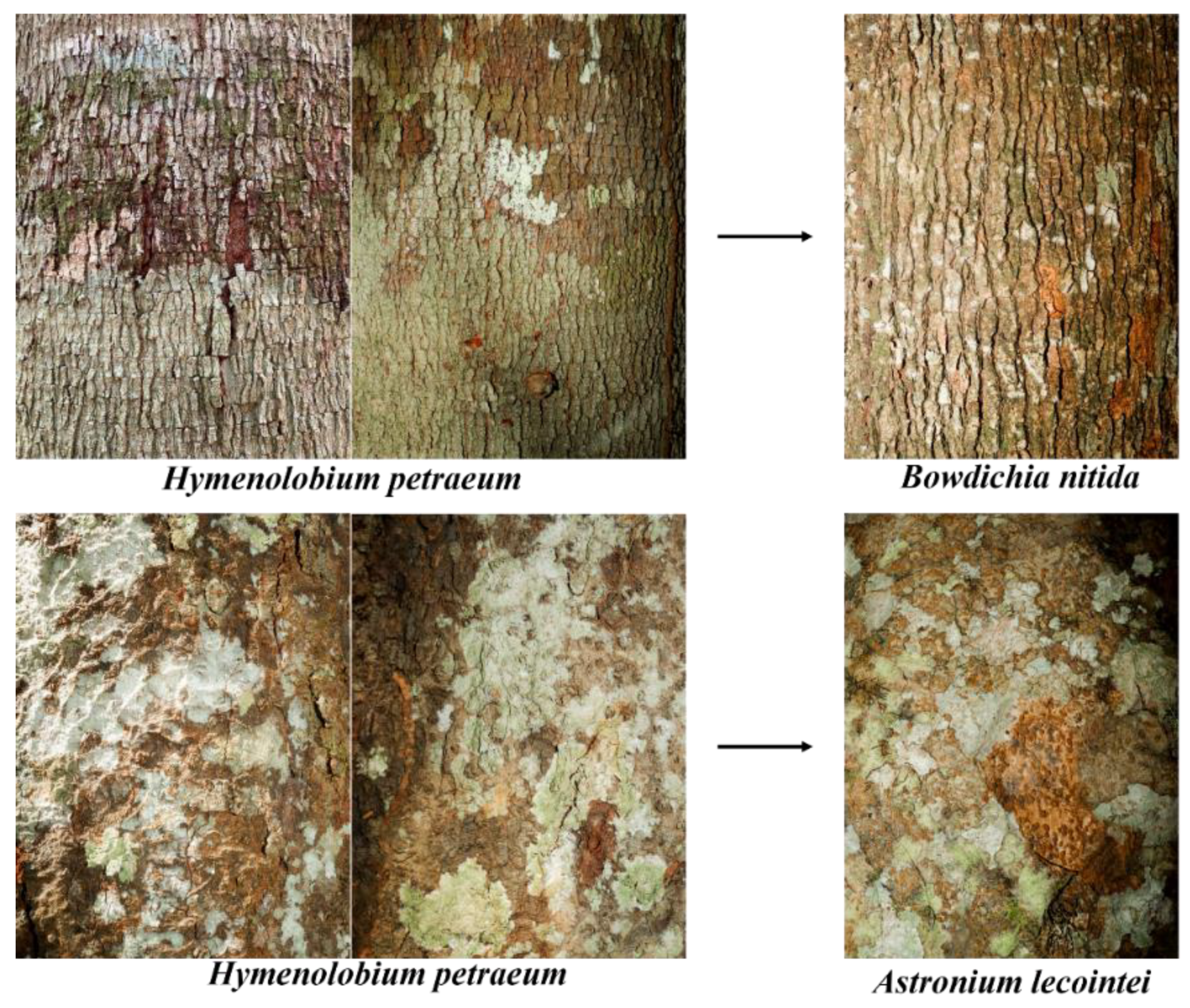
Figure 3 (a and b) present the confusion matrices for the best-performing classifiers: C6 ( and ANN) and ResNet50 with SVM, respectively. In the C6 model, Hymenolobium petraeum, Goupia glabra, and Dipteryx odorata showed higher misclassification rates. H. petraeum was mainly confused with Astronium lecointei and Bowdichia nítida; G. glabra with D. odorata, H. petraeum, Protium acrense, and Vatairea sericea; and D. odorata with Mezilaurus itauba. The ResNet50 + SVM classifier exhibited fewer errors, with notable confusion between D. odorata and Apuleia leiocarpa, and Parkia pendula and A. lecointei.
Figure 4 compares species-level recall between classifiers. The C6 model showed generally lower recall, especially for H. petraeum and G. glabra. In contrast, ResNet50 with SVM achieved higher recall across all species, reaching 100% accuracy for six of them.
4. Discussion
4.1. Images sets: characteristics, sources of variation and dificulties
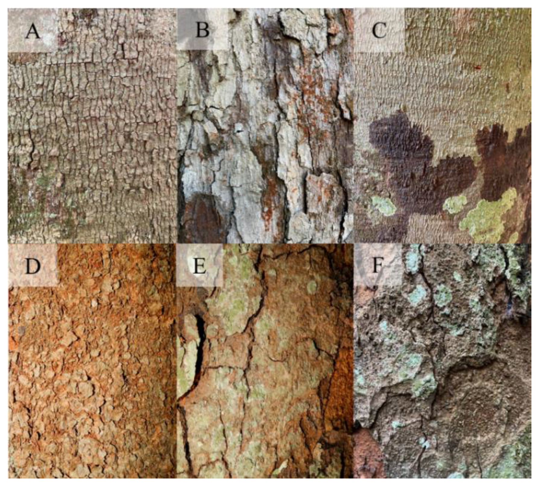
The “Amazon Bark” image set includes species exhibiting substantial intra- and interspecific variability in outer bark morphology (Refer to the Appendix A – Figure A4 for additional details).). Field observations indicate that bark structure is primarily influenced by tree size, with additional variation linked to humidity and diameter, both closely associated with tree age.
Image collection in tropical forests is hindered by operational challenges, notably inconsistent lighting due to understory shading and overexposure in open areas. These factors, coupled with morphological variability, complicate automated species recognition. Therefore, standardized protocols for image acquisition—regarding lighting, camera angle, and distance—are critical for effective field application of recognition systems.
These challenges also affect the reliability of forest inventories under Sustainable Forest Management (SFM), where accurate species identification is required for legal compliance and biodiversity monitoring. In Brazil, field inventories must comply with official protocols (e.g., IN nº 21/2014, IBAMA), and misidentification can result in illegal harvesting or misclassification of protected species.
4.2. Local Binary Standards
Although rotation-invariant uniform () is generally robust for texture classification, the non-invariant variant () outperformed it in this study, suggesting that bark texture orientation has limited influence on species discrimination, consistent with previous wood image classification research [11,59,60]. Early fusion of multiple LBP descriptors further enhanced feature representation and classification accuracy [61]; for example, alone achieved 66% accuracy, while combining , and improved accuracy by 6%.
The practical relevance of the superior performance of non-rotation-invariant uniform LBP lies in its computational efficiency and suitability for field applications. LBP-based models, particularly those applied to sub-image patches, demonstrated reasonably high accuracy and potential for rapid, low-cost species recognition in forest inventories. These models are especially advantageous in remote settings with limited computational resources, where deploying deep learning may be impractical.
However, their susceptibility to misclassification due to similar bark textures and environmental noise highlights the need for standardized imaging and proper lighting—challenges common in dense Amazonian forests. While promising for preliminary species filtering or flagging ambiguous cases, these models may require integration with morphological features or expert validation in regulatory frameworks.
From a policy perspective, LBP models could facilitate swift assessments during timber harvesting inspections, enhancing traceability and enforcement under Brazil’s Forest Code. By identifying likely misclassifications early, such tools can help forest agents and concession managers prioritize verification efforts, alleviating pressure on limited human resources in environmental monitoring.
4.3. Transfer learning
Numerous studies have confirmed the efficacy of pre-trained convolutional neural networks (CNNs) for plant classification across various structures, including leaves [47,62], wood [34,46,63,64], bark [18,65], and charcoal [39,66]. However, deep learning applications using bark images remain scarce [67], likely due to task complexity and limited access to large, high-quality datasets.
As established in the literature, larger datasets enhance model generalization and mitigate overfitting [68,69]. In this study, extracting 256 × 256 pixel sub-images from high-resolution bark images significantly improved classification accuracy across all CNN architectures, likely due to increased data volume and improved learning from fine-scale features.
This sub-image strategy, combined with majority voting, has also proven effective in related domains. [39] attained 95.7% accuracy with charcoal images from 44 forest species, and [70] reported 93% with wood images from 14 European species using similar methods. In the present study, ResNet50 coupled with either Artificial Neural Networks (ANN) or Support Vector Machines (SVM) yielded the best results, corroborating prior plant imaging research [71,72,73].
While dense neural networks are frequently applied to bark classification with strong performance [18,67,74,75], SVM slightly outperformed them in this study. Notably, Linear Discriminant Analysis (LDA) offered competitive accuracy (92%) with significantly reduced training time—two hours compared to over six for SVM—highlighting an efficient alternative [76].
Within the context of Sustainable Forest Management (SFM) in the Brazilian Amazon, this work marks a significant advancement toward a robust, generalizable bark-based species recognition system. The proposed model demonstrated high accuracy and holds potential to reduce identification errors during forest inventories, particularly for the 16 commercially important species assessed.
4.4. Implications for Sustainable Forest Management and Future Perspectives
Although the models achieved high classification performance, some misclassifications were noted, particularly in those using LBP descriptors. Visual similarities in bark traits—such as reticulated rhytidome and grey to brown color variation [77] —likely contributed to these errors, as did the presence of lichens. Comparable misclassifications occurred in ResNet50 and SVM models (Refer to the Appendix A – Figure A5 and A6 for additional details).
These findings highlight how morphological similarities, shaped by microenvironmental factors, can challenge species differentiation by automated classifiers. Environmental and structural factors—such as edaphoclimatic conditions, forest typology, and the sociological position of trees—are known to influence bark morphology.
These sources of variability highlight the need to expand both the taxonomic and morphological diversity of training datasets. Constructing a more generalizable recognition system requires not only the inclusion of additional species, but also a broader sampling effort that captures individual variability within species. Sampling strategies based on the diameter distribution of each species could improve representativeness, though this remains a complex task in Amazonian forests.
From a practical standpoint, the adoption of automated species recognition tools in SFM operations has clear benefits. By minimizing taxonomic errors during forest inventories, such systems can increase the accuracy of management plans, enhance compliance with legal frameworks such as Brazil’s Forest Code, and reduce the risk of unauthorized logging. Furthermore, they offer potential for supporting biodiversity monitoring and long-term ecological assessments by facilitating large-scale, standardized species identification.
To ensure operational viability, future work should prioritize:
- Expansion of datasets to include regional and structural bark variability;
- Validation of models using mobile devices under field conditions;
- Integration of other plant organs (e.g., leaves, fruits) for multimodal classification;
- Development of lightweight architectures for deployment in remote forest environments.
This study also contributes to the operationalization of automated tools for SFM. Reliable species recognition supports legal compliance, inventory planning, and biodiversity monitoring. While current limitations include a restricted number of species and high computational demand, the system shows clear potential for practical use in forest governance.
5. Conclusions
This study represents a step forward in automated species identification within the framework of Sustainable Forest Management (SFM) in the Brazilian Amazon, where accurate botanical identification is critical yet often hindered by operational and taxonomic limitations. By using bark sub-image analysis and deep learning models—particularly ResNet50 combined with classifiers such as SVM and ANN—the system achieved up to 95% accuracy in identifying 16 commercial timber species, demonstrating both technical feasibility and field scalability.
Despite these promising results, practical deployment requires expanding species coverage, validating models in real-world settings, and developing lightweight versions suitable for mobile devices. Integration with official forest inventory platforms and updated taxonomic databases could enhance traceability within the timber supply chain, reduce identification errors, and support compliance with environmental regulations and international commitments. Thus, the proposed models show strong potential as complementary tools for data-driven tropical forest management.
Author Contributions
Conceptualization, N.C.G., L.E.S.O., S.d.P.C.e.C. and D.V.S.; methodology, N.C.G., L.E.S.O., S.d.P.C.e.C. and D.V.S.; software, N.C.G., L.E.S.O. and D.V.S.; validation, N.C.G., L.E.S.O., S.d.P.C.e.C., A.B., P.L.d.P.F., E.d.S.L. and D.V.S.; formal analysis, N.C.G., L.E.S.O., S.d.P.C.e.C., A.B., P.L.d.P.F., E.d.S.L. and D.V.S.; investigation, N.C.G., S.d.P.C.e.C., M.O.d.S.H., E.d.S.L. and D.V.S; resources, S.d.P.C.e.C., M.O.d.S.H. and E.d.S.L.; data curation, N.C.G. and D.V.S.; writing—original draft preparation, N.C.G.; writing—review and editing, N.C.G., L.E.S.O., S.d.P.C.e.C., A.B., P.L.d.P.F. and D.V.S.; visualization, N.C.G., L.E.S.O. and D.V.S.; supervision, L.E.S.O., S.d.P.C.eC., A.B. and D.V.S.; project administration, S.d.P.C.e.C. and D.V.S.; funding acquisition, S.d.P.C.e.C and D.V.S. All authors have read and agreed to the published version of the manuscript.
Funding
This work was supported by the Center of Wood Producing and Exporting Industries of the State of Mato Grosso (CWPEISMG), with administrative and financial intervention from the Foundation for Research and Development Support (FADESP).
Data Availability Statement
The dataset used in this study is not yet publicly available, as it represents the first stage of the “Deep Flora” project. In future stages, the dataset is expected to be expanded to include a greater diversity of flora species and subsequently made publicly accessible. However, the data may be provided by the corresponding author upon reasonable request. All source codes developed during the research are openly available at: https://github.com/NatallyCelestino/Bark_Recogition.git.
Acknowledgments
The authors gratefully acknowledge the financial and institutional support provided by the Center of Timber Producing and Exporting Industries of Mato Grosso (CIPEM), which was essential for the development of this research.
Conflicts of Interest
The authors declare that they have no known competing financial interests or personal relationships that could have appeared to influence the work reported in this paper.
Appendix A
Appendix A.1
Figure A1.
Representation of the collection procedures for the construction of the set of bark images of commercial trees of Amazonian forest species.
Figure A1.
Representation of the collection procedures for the construction of the set of bark images of commercial trees of Amazonian forest species.
Appendix A.2
Figure A2.
(A) low-light area; (B) use of the reflector.

Appendix A.3
Figure A3.
(A) climbing and collecting botanical material; (B) assembling the exsiccates.
Appendix A.4
Figure A4.
Images of different trees of Trattinnickia burserifolia (A, B and C) and Parkia pendula (D, E and F).
Figure A4.
Images of different trees of Trattinnickia burserifolia (A, B and C) and Parkia pendula (D, E and F).
Appendix A.5
Figure A5.
Images of the species Hymenolobium petraeum that were misclassified as Bowdichia nítida and Astronium lecointei by the C6 classifier ( e ANN).
Figure A5.
Images of the species Hymenolobium petraeum that were misclassified as Bowdichia nítida and Astronium lecointei by the C6 classifier ( e ANN).
Appendix A.6
Figure A6.
Images of the species Hymenolobium petraeum and Dipteryx odorata that were misclassified as Apuleia leiocarpa by the classifier built using ResNet50 and SVM.
Figure A6.
Images of the species Hymenolobium petraeum and Dipteryx odorata that were misclassified as Apuleia leiocarpa by the classifier built using ResNet50 and SVM.
Appendix A.7

Table A1.
Candidate hyperparameters for each machine learning algorithm.
| Algorithm | Candidate Hyperparameters |
| Artificial neural networks |
hidden_layer_sizes = (50), (100), (150), (200), (250), (300), (350), (400), (450) e (500) |
| activation = relu e identity | |
| solver = adam e lbfgs | |
| alpha = uniform(loc = 0.0001, scale = 0.09).rvs(size = 20, random_state = 10) | |
| learning_rate = constant, adaptive e invscaling | |
| Support vector machine | C = uniform(loc = 0.1, scale = 10).rvs(size = 20, random_state = 10) |
| kernel = linear, rbf, poly e sigmoid | |
| degree = 2, 3 e 4 | |
| gamma = scale e auto + list(np.logspace(-9, 3, 13) | |
| Random forest | n_estimators = np.arange(40, 320, 20) |
| max_depth = list(np.arange(10, 100, step=10)) + [None] | |
| max_features = list(np.arange(30, 60, 5)) + [‘sqrt’, “log2”] | |
| criterion = gini e entropy | |
| min_samples_leaf = np.arange(10, 110, 10) | |
| min_samples_split = np.arange(2, 10, 2) | |
| bootstrap = True e False | |
| Linear discriminant analysis | solver = lsqr e eigen |
| tol = 0.0001, 0.0002 e 0.0003 |
Where: hidden_layer_sizes: number of neurons in each hidden layer; activation: activation function; solver: optimization algorithm used to update the network weights during training; alpha: penalty or regularization applied to the network weights; learning_rate: learning rate; C: controls the regularization of the model; kernel: type of function to be used in the algorithm to map the data to a higher-dimensional feature space; degree: used only for the polynomial kernel defining the degree of the polynomial; gamma: used for all kernels except linear; n_estimators: number of trees in the forest; max_depth: maximum depth of each tree; max_features: maximum number of features; criterion: defines the function to measure the quality of the split in a decision tree; min_samples_leaf: minimum number of samples needed to be a leaf in a tree; min_samples_split: minimum number of samples needed to split a node; bootstrap: indicates whether the samples are sampled with replacement (True) or not (False); tol: tolerance parameter.
References
- Loyola, R.; Machado, N.; Nova, D.V.; Martins, E.; Martinelli, G. Áreas Prioritárias Para Conservação e Uso Sustentável Da Flora Brasileira Ameaçada de Extinção; 2014; ISBN 978-85-88742-67-3.
- The Brazil Flora Group, B. Flora Do Brasil 2020. Jard. Botânico do Rio Janeiro, http://floradobrasil.jbrj.gov.br/Access 19 Set 2. 2021. [Google Scholar] [CrossRef]
- Melo, R.R. de; Rocha, M.J.; Rodolfo Junior, F.; Stangerlin, D.M. Análise Da Influência Do Diâmetro No Rendimento Em Madeira Serrada de Cambará (Qualea Sp.). Pesqui. Florest. Bras. 2017, 36, 393. [Google Scholar] [CrossRef]
- Stragliotto, M.C.; Pereira, B.L.C.; Oliveira, A.C. Indústrias Madeireiras E Rendimento Em Madeira Serrada Na Amazônia Brasileira. Eng. Florest. Desafios, Limites e Potencialidade. [CrossRef]
- CONAMA Brasil, Ministério Do Meio Ambiente. Resolução CONAMA No 406 de 02 de Fevereiro de 2009. 2009, 1–5.
- Hadlich, H.L.; Durgante, F.M.; dos Santos, J.; Higuchi, N.; Chambers, J.Q.; Vicentini, A. Recognizing Amazonian Tree Species in the Field Using Bark Tissues Spectra. For. Ecol. Manage. 2018, 427, 296–304. [Google Scholar] [CrossRef]
- Encinas, J.I.; Antônio, M.; Ferreira, C.; Riesco, G.; Alboreca, A.R. Introduction Forest Management in the Sustained Yield Regime Considers That in the Management. 13. [CrossRef]
- Engel, J.; Brousseau, L.; Baraloto, C. GuiaTreeKey, a Multi-Access Electronic Key to Identify Tree Genera in French Guiana. 44, 44. [CrossRef]
- Lang, C.; Almeida, D.R.A.; Costa, F.R.C. Discrimination of Taxonomic Identity at Species, Genus and Family Levels Using Fourier Transformed Near-Infrared Spectroscopy (FT-NIR). For. Ecol. Manage. 2017, 406, 219–227. [Google Scholar] [CrossRef]
- Procópio, L.C.; Secco, R.D.S. A Importância Da Identificação Botânica Nos Inventários Florestais: O Exemplo Do “Tauari” (Couratari Spp. e Cariniana Spp. - Lecythidaceae) Em Duas Áreas Manejadas No Estado Do Pará. Acta Amaz. 2008, 38, 31–44. [Google Scholar] [CrossRef]
- Venicio, D.; Joielan, S.; Santos, X.; Cristina, H.; Lorena, T.; Silvana, N.; Luiz, N.; Oliveira, E.S. An Automatic Recognition System of Brazilian Flora Species Based on Textural Features of Macroscopic Images of Wood. Wood Sci. Technol. 2020, 54, 1065–1090. [Google Scholar] [CrossRef]
- Menezes, M.; Bicudo, C.E.M.; Moura, C.W.N.; Alves, A.M.; Santos, A.A.; Pedrini, A. de G.; Araújo, A.; Tucci, A.; Fajar, A.; Malone, C.; et al. Update of the Brazilian Floristic List of Algae and Cyanobacteria. Rodriguésia 2015, 66, 1047–1062. [Google Scholar] [CrossRef]
- Novaes1, T.V.; Ramalho, F.M.G.; da Silva Araujo, E.; Lima, M.D.R.; da Silva, M.G.; Ferreira, G.C.; Hein, P.R.G. Discrimination of Amazonian Forest Species by NIR Spectroscopy: Wood Surface Effects. Eur. J. Wood Wood Prod. 2023, 81, 159–172. [Google Scholar] [CrossRef]
- Lacerda, A.E.B. de; Nimmo, E.R. Can We Really Manage Tropical Forests without Knowing the Species within? Getting Back to the Basics of Forest Management through Taxonomy. For. Ecol. Manage. 2010, 259, 995–1002. [Google Scholar] [CrossRef]
- Cysneiros, V.C.; Mendonça Júnior, J.O.; Lanza, T.R.; Moraes, J.C.R.; Samor, O.J.M. Espécies Madeireiras Da Amazônia: Riqueza, Nomes Populares e Suas Peculiaridades. Pesqui. Florest. Bras. 2018, 38. [Google Scholar] [CrossRef]
- Ferreira, R.L.A.; Cerqueira, R.M.; Cardoso Junior, R.C. Análise Da Identificação Botânica Em Inventários Florestais de Planos de Manejo Sustentáveis No Oeste Paraense. Nat. Conserv. 2020, 13, 136–145. [Google Scholar] [CrossRef]
- Filho, P.L.P.; Oliveira, L.S.; Nisgoski, S.; Britto, A.S. Forest Species Recognition Using Macroscopic Images. Mach. Vis. Appl. 2014, 25, 1019–1031. [Google Scholar] [CrossRef]
- Carpentier, M.; Giguere, P.; Gaudreault, J. Tree Species Identification from Bark Images Using Convolutional Neural Networks. In Proceedings of the 2018 IEEE/RSJ International Conference on Intelligent Robots and Systems (IROS); IEEE, October 2018; pp. 1075–1081. [Google Scholar]
- Gogul, I.; Kumar, V.S. Flower Species Recognition System Using Convolution Neural Networks and Transfer Learning. In Proceedings of the 2017 Fourth International Conference on Signal Processing, March 2017, Communication and Networking (ICSCN); IEEE; pp. 1–6.
- Ghosh, A.; Roy, P. An Automated Model for Leaf Image-Based Plant Recognition: An Optimal Feature-Based Machine Learning Approach. Innov. Syst. Softw. Eng. 2022. [Google Scholar] [CrossRef]
- Ran, J.; Shi, Y.; Yu, J.; Li, D. A Multi-Feature Convolution Neural Network for Automatic Flower Recognition. J. Circuits, Syst. Comput. 2021, 30, 1–15. [Google Scholar] [CrossRef]
- Anubha Pearline, S.; Sathiesh Kumar, V.; Harini, S. A Study on Plant Recognition Using Conventional Image Processing and Deep Learning Approaches. J. Intell. Fuzzy Syst. 2019, 36, 1997–2004. [Google Scholar] [CrossRef]
- Kaya, A.; Keceli, A.S.; Catal, C.; Yalic, H.Y.; Temucin, H.; Tekinerdogan, B. Analysis of Transfer Learning for Deep Neural Network Based Plant Classification Models. Comput. Electron. Agric. 2019, 158, 20–29. [Google Scholar] [CrossRef]
- Kumar, M. Plant Species Recognition Using Morphological Features and Adaptive Boosting Methodology. IEEE Access 2019, 7, 163912–163918. [Google Scholar] [CrossRef]
- Turkoglu, M.; Hanbay, D. Leaf-Based Plant Species Recognition Based on Improved Local Binary Pattern and Extreme Learning Machine. Phys. A Stat. Mech. its Appl. 2019, 527, 121297. [Google Scholar] [CrossRef]
- Keivani, M.; Mazloum, J.; Sedaghatfar, E.; Tavakoli, M.B. Automated Analysis of Leaf Shape, Texture, and Color Features for Plant Classification. Trait. du Signal 2020, 37, 17–28. [Google Scholar] [CrossRef]
- Bisen, D. Deep Convolutional Neural Network Based Plant Species Recognition through Features of Leaf. Multimed. Tools Appl. 2021, 80, 6443–6456. [Google Scholar] [CrossRef]
- Wang, B.; Li, H.; You, J.; Chen, X.; Yuan, X.; Feng, X. Fusing Deep Learning Features of Triplet Leaf Image Patterns to Boost Soybean Cultivar Identification. Comput. Electron. Agric. 2022, 197, 106914. [Google Scholar] [CrossRef]
- Misra, D.; Crispim-Junior, C.; Tougne, L. Patch-Based CNN Evaluation for Bark Classification. In; 2020; pp. 197–212 ISBN 9783030654146.
- Remeš, V.; Haindl, M. Bark Recognition Using Novel Rotationally Invariant Multispectral Textural Features. Pattern Recognit. Lett. 2019, 125, 612–617. [Google Scholar] [CrossRef]
- Bertrand, S.; Cerutti, G.; Tougne, L. Bark Recognition to Improve Leaf-Based Classification in Didactic Tree Species Identification. In Proceedings of the Proceedings of the 12th International Joint Conference on Computer Vision, Imaging and Computer Graphics Theory and Applications.
- Geus, A.R. de; Backes, A.R.; Gontijo, A.B.; Albuquerque, G.H.Q.; Souza, J.R. Amazon Wood Species Classification: A Comparison between Deep Learning and Pre-Designed Features. Wood Sci. Technol. 2021, 55, 857–872. [Google Scholar] [CrossRef]
- Taslim, A.; Saon, S.; Mahamad, A.K.; Muladi, M.; Hidayat, W.N. Plant Leaf Identification System Using Convolutional Neural Network. Bull. Electr. Eng. Informatics 2021, 10, 3341–3352. [Google Scholar] [CrossRef]
- He, J.; Sun, Y.; Yu, C.; Cao, Y.; Zhao, Y.; Du, G. An Improved Wood Recognition Method Based on the One-Class Algorithm. Forests 2022, 13, 1350. [Google Scholar] [CrossRef]
- Thanikkal, J.G.; Dubey, A.K.; Thomas, M.T. An Efficient Mobile Application for Identification of Immunity Boosting Medicinal Plants Using Shape Descriptor Algorithm. Wirel. Pers. Commun. 2023, 131, 1189–1205. [Google Scholar] [CrossRef] [PubMed]
- Silveira, A.B. da; Santos, J. de P. dos; Rebellato, L. Guia de Boas Práticas: Restauração de Áreas de Preservação Permanente Degradadas (APPDs), Experiência Da Fazenda São Nicolau; 2017; ISBN 978-85-94211-00-2. [Google Scholar]
- Borges, H.B.N.; Silveira, E.A.; Vendramin, L.N. Flora Arbórea de Mato Grosso - Tipologia Vegetais e Suas Éspecies; 2014; ISBN 978-85-7992-072-1.
- Benini, R.; Santana, P.; Borgo, M.; Girão, V.; Campos, M.; Klein, F.; Kummer, O.P.; Netto, D.S. de A.; Rodrigues, R.R.; Nave, A.G.; et al. Manual De Restauração Da Vegetação Nativa, Alto Teles Pires, Mt Expediente. 2016, 136.
- Maruyama, T.M.; Oliveira, L.S.; Britto, A.S.; Nisgoski, S. Automatic Classification of Native Wood Charcoal. Ecol. Inform. 2018, 46, 1–7. [Google Scholar] [CrossRef]
- Robert, M.; Dallaire, P.; Giguere, P. Tree Bark Re-Identification Using a Deep-Learning Feature Descriptor. Proc. - 2020 17th Conf. Comput. Robot Vision, CRV 2020, 32. [CrossRef]
- Ojala, T.; Pietikhenl, M.; Harwood, D. Performance Evaluation of Texture Measures with Classification Based on Kullback Discrimination of Distributions. 1994, 582–585.
- Ojala, T.; Pietikainen, M.; Maenpaa, T. Multiresolution Gray-Scale and Rotation Invariant Texture Classification with Local Binary Patterns. IEEE Trans. Pattern Anal. Mach. Intell. 2002, 24, 971–987. [Google Scholar] [CrossRef]
- Li, J.; Sun, S.; Jiang, H.; Tian, Y.; Xu, X. Image Recognition and Empirical Application of Desert Plant Species Based on Convolutional Neural Network. J. Arid Land 2022, 14, 1440–1455. [Google Scholar] [CrossRef]
- Huang, Z.; He, C.; Wang, Z.-N.; Xi, J.; Wang, H.; Hou, L. Cinnamomum Camphora Classification Based on Leaf Image Using Transfer Learning. In Proceedings of the 2019 IEEE 4th Advanced Information Technology, December 2019, Electronic and Automation Control Conference (IAEAC); IEEE; pp. 1426–1429.
- Cai, X.; Huo, Y.; Chen, Y.; Xi, M.; Tu, Y.; Sun, C.; Sun, H. Real-Time Leaf Recognition Method Based on Image Segmentation and Feature Extraction. Int. J. Pattern Recognit. Artif. Intell. 2022, 36, 1–24. [Google Scholar] [CrossRef]
- Figueroa-Mata, G.; Mata-Montero, E.; Valverde-Otárola, J.C.; Arias-Aguilar, D.; Zamora-Villalobos, N. Using Deep Learning to Identify Costa Rican Native Tree Species From Wood Cut Images. Front. Plant Sci. 2022, 13, 1–12. [Google Scholar] [CrossRef] [PubMed]
- Zhang, R.; Zhu, Y.; Ge, Z.; Mu, H.; Qi, D.; Ni, H. Transfer Learning for Leaf Small Dataset Using Improved ResNet50 Network with Mixed Activation Functions. Forests 2022, 13, 2072. [Google Scholar] [CrossRef]
- Soni, P.; Dhavale, S.; Yenishetti, S.; Panat, L.; Karajkhede, G. Medicinal Plant Species Identification Using AI. In Proceedings of the 2023 IEEE 11th Region 10 Humanitarian Technology Conference (R10-HTC); IEEE, October 16 2023; pp. 662–668. [Google Scholar]
- Kini, A.S.; Prema, K. V.; Pai, S.N. Early Stage Black Pepper Leaf Disease Prediction Based on Transfer Learning Using ConvNets. Sci. Rep. 2024, 14, 1404. [Google Scholar] [CrossRef] [PubMed]
- Faisal, S.; Javed, K.; Ali, S.; Alasiry, A.; Marzougui, M.; Khan, M.A.; Cha, J.H. Deep Transfer Learning Based Detection and Classification of Citrus Plant Diseases. Comput. Mater. Contin. 2023, 76, 895–914. [Google Scholar] [CrossRef]
- Thirumala, K.; Pal, S.; Jain, T.; Umarikar, A.C. Neurocomputing A Classification Method for Multiple Power Quality Disturbances Using EWT Based Adaptive Filtering and Multiclass SVM. Neurocomputing 2019, 334, 265–274. [Google Scholar] [CrossRef]
- Toğaçar, M.; Ergen, B.; Cömert, Z. Classification of Flower Species by Using Features Extracted from the Intersection of Feature Selection Methods in Convolutional Neural Network Models. Measurement 2020, 158, 107703. [Google Scholar] [CrossRef]
- Dourado Filho, L.A.; Calumby, R.T. Data Augmentation Policies and Heuristics Effects over Dataset Imbalance for Developing Plant Identification Systems Based on Deep Learning: A Case Study. Rev. Bras. Comput. Apl. 2022, 14, 85–94. [Google Scholar] [CrossRef]
- Nunes, M.H.; Görgens, E.B. Artificial Intelligence Procedures for Tree Taper Estimation within a Complex Vegetation Mosaic in Brazil. PLoS One 2016, 11, e0154738. [Google Scholar] [CrossRef] [PubMed]
- Fan, G.; Yu, M.; Dong, S.; Yeh, Y.; Hong, W. Forecasting Short-Term Electricity Load Using Hybrid Support Vector Regression with Grey Catastrophe and Random Forest Modeling. Util. Policy 2021, 73, 101294. [Google Scholar] [CrossRef]
- Sahu, S.K.; Pandey, M. Machine Translated by Google Sistemas Especialistas Com Aplicações Um SVM Multiclasse Híbrido Ideal Para Detecção de Doenças Foliares de Plantas Usando o Modelo Espacial Fuzzy C-Means. 2023, 214, 0–1.
- Rosa, A.C.F. da; Galdamez, E.V.C.; Souza, R.C.T. de; Melo, M. das G.M.; Villarinho, A.L.C.F.; Leal, G.C.L. Uso de Técnicas de Aprendizado de Máquina Para Classificação de Fatores Que Influenciam a Ocorrência de Dermatites Ocupacionais. Rev. Bras. Saúde Ocup. 2023, 48, 1–10. [Google Scholar] [CrossRef]
- Wu, Q.; Luo, J.; Fang, H.; He, D.; Liang, T. Spectral Classification Analysis of Recycling Plastics of Small Household Appliances Based on Infrared Spectroscopy. Vib. Spectrosc. 2024, 130, 103636. [Google Scholar] [CrossRef]
- Paula, P.L.; Luiz, F.; Silvana, S.O.; Alceu, N.; Jr, S.B. Reconhecimento de Espécies Florestais Usando Imagens Macroscópicas. 2014. [Google Scholar] [CrossRef]
- Rahiddin, R.N.N.; Hashim, U.R.; Salahuddin, L.; Kanchymalay, K.; Wibawa, A.P.; Chun, T.H. Local Texture Representation for Timber Defect Recognition Based on Variation of LBP. Int. J. Adv. Comput. Sci. Appl. 2022, 13, 443–448. [Google Scholar] [CrossRef]
- Tortorici, C.; Werghi, N. Early Features Fusion over 3D Face for Face Recognition. In; Ben Amor, B., Chaieb, F., Ghorbel, F., Eds.; Communications in Computer and Information Science; Springer International Publishing: Cham, 2017; ISBN 978-3-319-60653-8. [Google Scholar]
- Vizcarra, G.; Bermejo, D.; Mauricio, A.; Zarate Gomez, R.; Dianderas, E. The Peruvian Amazon Forestry Dataset: A Leaf Image Classification Corpus. Ecol. Inform. 2021, 62, 101268. [Google Scholar] [CrossRef]
- Ravindran, P.; Owens, F.C.; Wade, A.C.; Shmulsky, R.; Wiedenhoeft, A.C. Towards Sustainable North American Wood Product Value Chains, Part I: Computer Vision Identification of Diffuse Porous Hardwoods. Front. Plant Sci. 2022, 12, 1–13. [Google Scholar] [CrossRef] [PubMed]
- Yang, Y.; Wang, H.; Jiang, D.; Hu, Z. Surface Detection of Solid Wood Defects Based on SSD Improved with ResNet. Forests 2021, 12, 1419. [Google Scholar] [CrossRef]
- Kim, T.K.; Hong, J.; Ryu, D.; Kim, S.; Byeon, S.Y.; Huh, W.; Kim, K.; Baek, G.H.; Kim, H.S. Identifying and Extracting Bark Key Features of 42 Tree Species Using Convolutional Neural Networks and Class Activation Mapping. Sci. Rep. 2022, 12, 4772. [Google Scholar] [CrossRef] [PubMed]
- Menon, L.T.; Laurensi, I.A.; Penna, M.C.; Oliveira, L.E.S.; Britto, A.S. Data Augmentation and Transfer Learning Applied to Charcoal Image Classification. In Proceedings of the 2019 International Conference on Systems, June 2019; Vol. 2019-June, Signals and Image Processing (IWSSIP); IEEE; pp. 69–74.
- Cui, L.; Chen, S.; Mu, Y.; Xu, X.; Zhang, B.; Zhao, X. Tree Species Classification over Cloudy Mountainous Regions by Spatiotemporal Fusion and Ensemble Classifier. Forests 2023, 14, 107. [Google Scholar] [CrossRef]
- Khosla, C.; Saini, B.S. Enhancing Performance of Deep Learning Models with Different Data Augmentation Techniques : A Survey. 2020. [Google Scholar] [CrossRef]
- Nanni, L.; Paci, M.; Brahnam, S.; Lumini, A. Comparison of Different Image Data Augmentation Approaches. J. Imaging 2021, 7, 254. [Google Scholar] [CrossRef] [PubMed]
- Fabijańska, A.; Danek, M.; Barniak, J. Wood Species Automatic Identification from Wood Core Images with a Residual Convolutional Neural Network. Comput. Electron. Agric. 2021, 181, 105941. [Google Scholar] [CrossRef]
- Durairajah, V.; Gobee, S.; Muneer, A. Automatic Vision Based Classification System Using DNN and SVM Classifiers. In Proceedings of the 2018 3rd International Conference on Control, September 2018, Robotics and Cybernetics (CRC); IEEE; pp. 6–14.
- Zhao, Y.; Gao, X.; Hu, J.; Chen, Z. Tree Species Identification Based on the Fusion of Bark and Leaves. Math. Biosci. Eng. 2020, 17, 4018–4033. [Google Scholar] [CrossRef] [PubMed]
- Diwedi, H.K.; Misra, A.; Tiwari, A.K. CNN-Based Medicinal Plant Identification and Classification Using Optimized SVM; Springer US, 2024; Vol. 83; ISBN 0123456789.
- Ido, J.; Saitoh, T. CNN-Based Tree Species Identification from Bark Image. In Proceedings of the Tenth International Conference on Graphics and Image Processing (ICGIP 2018); Yu, H., Pu, Y., Li, C., Pan, Z., Eds.; SPIE, May 6 2019; p. 63. [Google Scholar]
- Faizal, S. Automated Identification of Tree Species by Bark Texture Classification Using Convolutional Neural Networks. Int. J. Res. Appl. Sci. Eng. Technol. 2022, 10, 1384–1392. [Google Scholar] [CrossRef]
- Sachar, S.; Kumar, A. Survey of Feature Extraction and Classification Techniques to Identify Plant through Leaves. Expert Syst. Appl. 2021, 167, 114181. [Google Scholar] [CrossRef]
- Ferreira, C.A.; Silva, H.D. da Eucalyptus Para a Região Amazônica, Estados de Rondônia e Acre. Embrapa Florestas 2004, 1, 1–4. [Google Scholar]
Figure 1.
Location of the three Demonstrative Units (DUs) of Forest Management in the state of Mato Grosso, Brazil – Farm Pérola (Nova Maringá), DU2 – Farm Boa Esperança (Feliz Natal), and DU3 – Farm São Nicolau (Cotriguaçu).
Figure 1.
Location of the three Demonstrative Units (DUs) of Forest Management in the state of Mato Grosso, Brazil – Farm Pérola (Nova Maringá), DU2 – Farm Boa Esperança (Feliz Natal), and DU3 – Farm São Nicolau (Cotriguaçu).
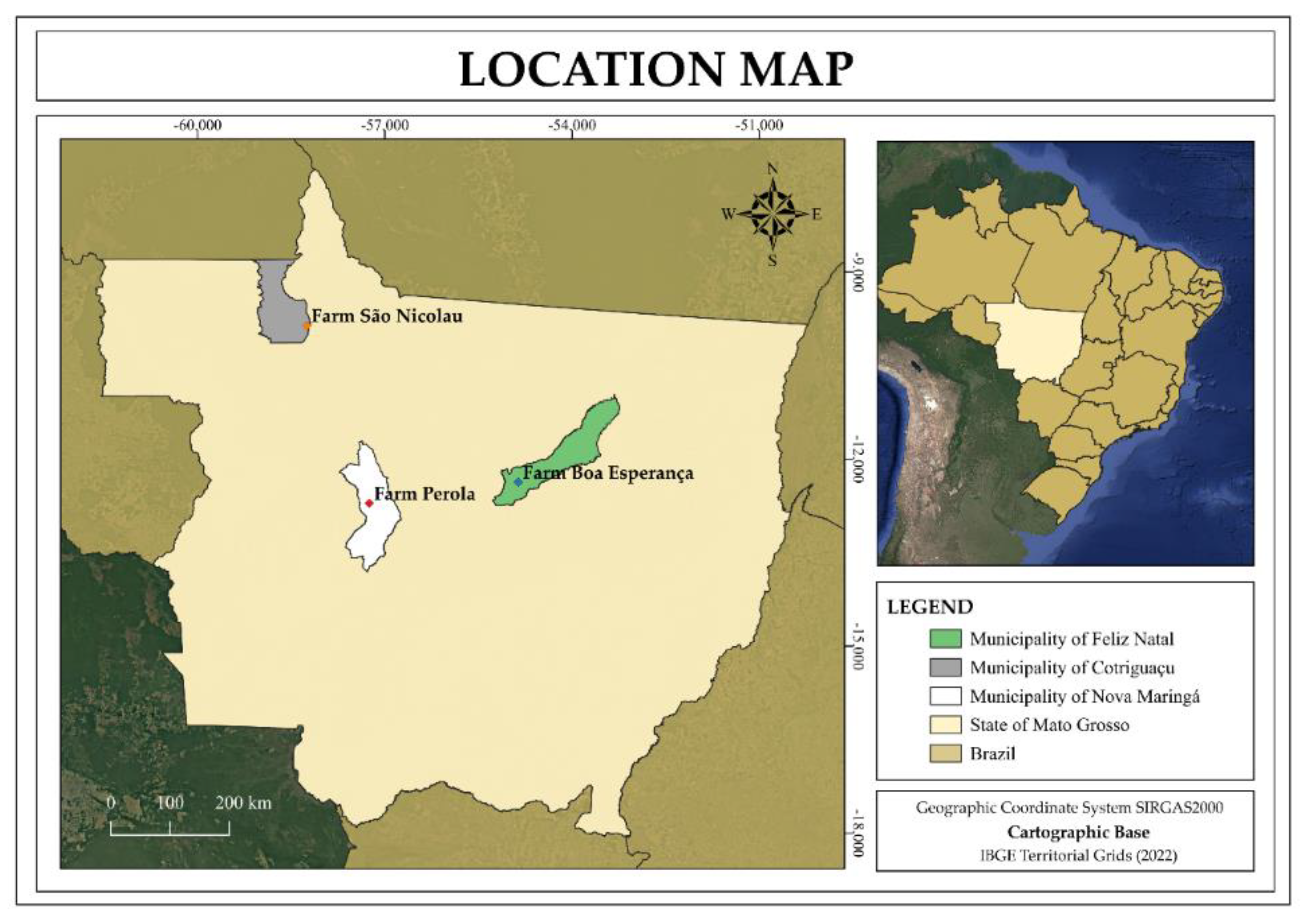
Figure 2.
Sample images of the bark of the 16 Amazonian forest species collected.
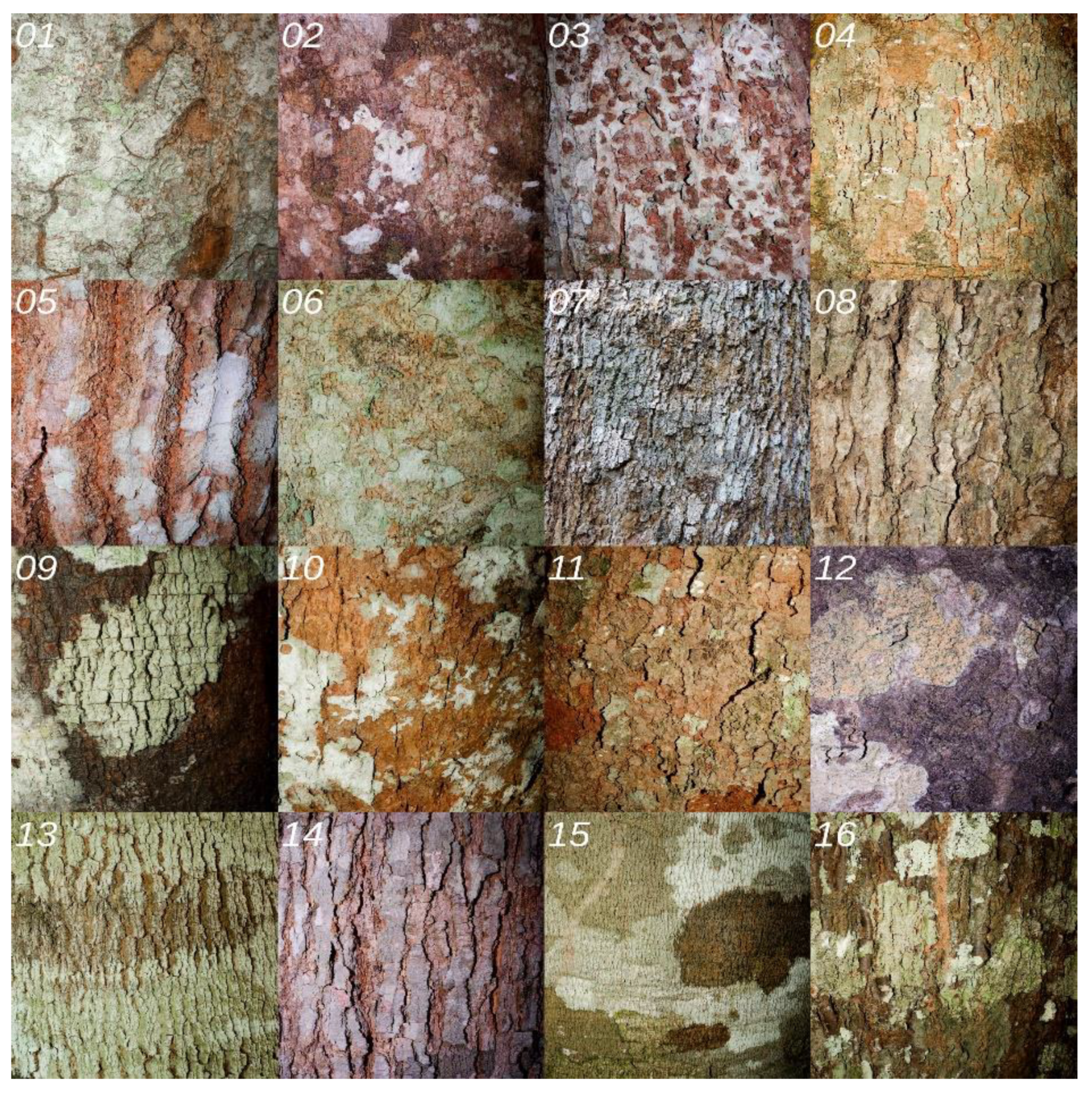
Figure 3.
(a) Confusion matrix in the C6 classifier test set, constructed using feature vectors of sub-images extracted by the operator and the multilayer neural network algorithm. (b) Confusion matrix in the test set for the classifier built using ResNet50 as the sub-image feature extractor and SVM as the classification algorithm.
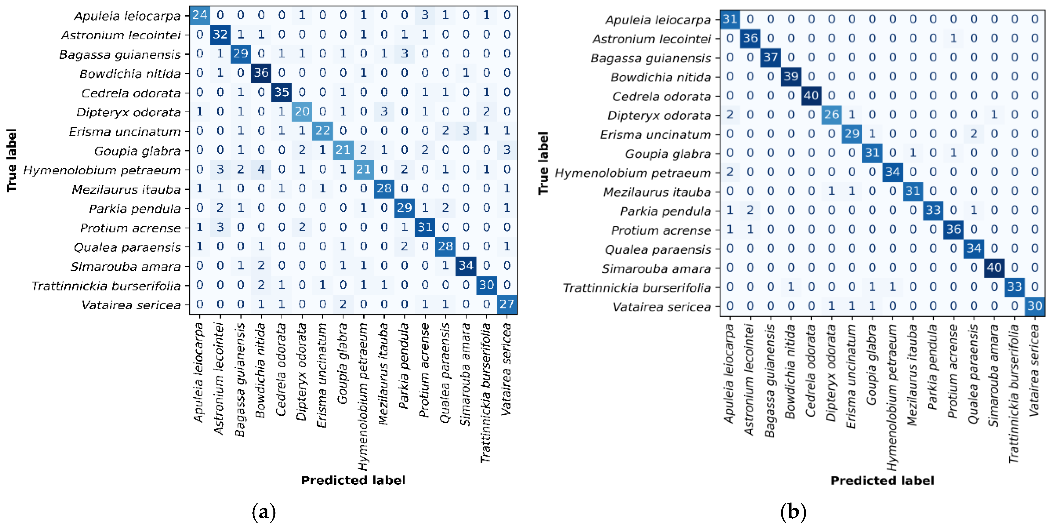
Figure 4.
Recognition rate per species (recall), on the test set, for the classifiers ( and ANN - classifier C6) and ResNet50 with SVM, built from sub-images.
Figure 4.
Recognition rate per species (recall), on the test set, for the classifiers ( and ANN - classifier C6) and ResNet50 with SVM, built from sub-images.
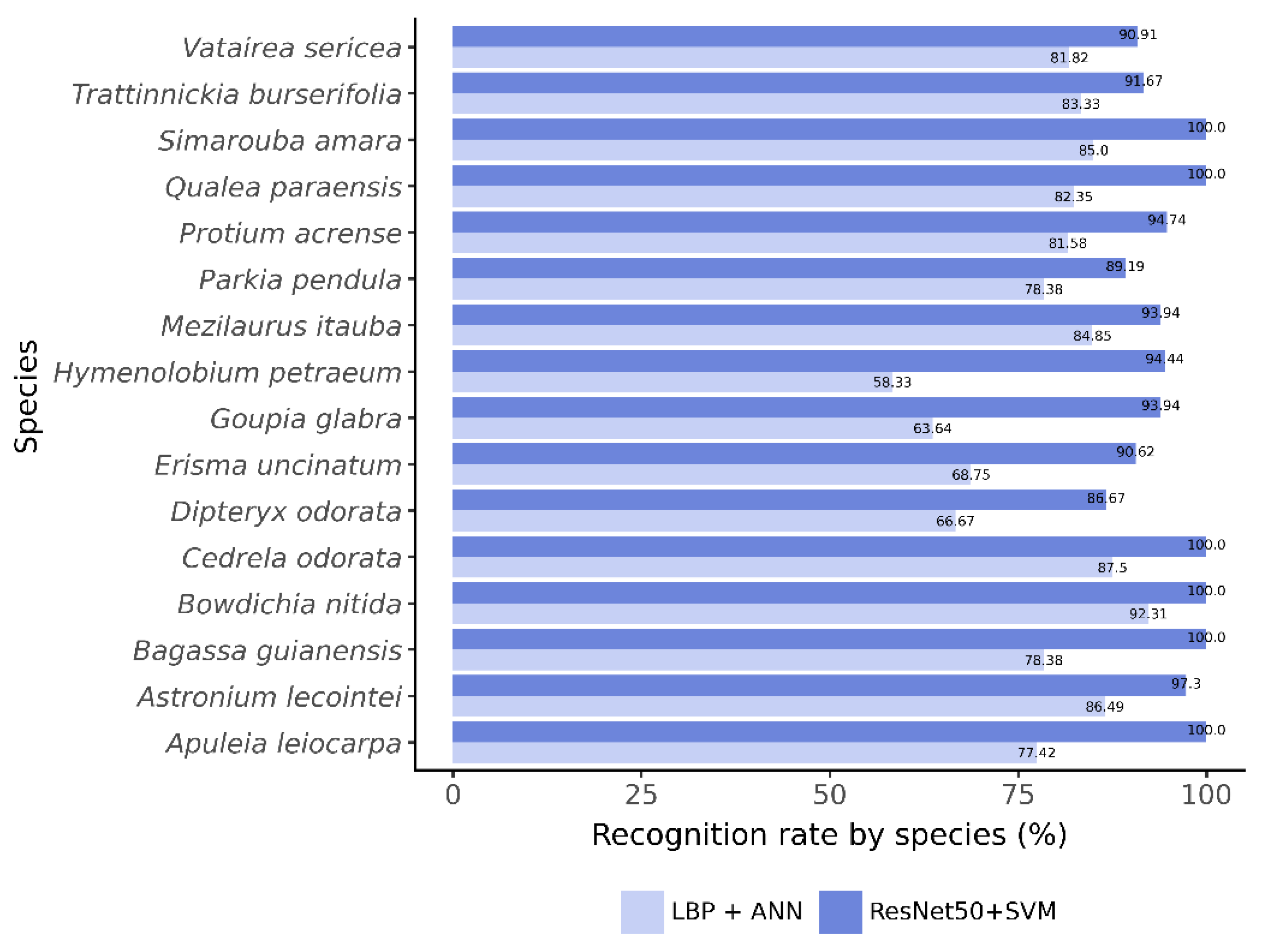
Table 1.
Family, scientific name, vernacular name, number of samples, and images (n) per species.
| ID1 | Family | Scientific name | Vernacular name | Samples | N2 |
| 1 | Fabaceae | Apuleia leiocarpa (Vogel) J. F. Macbr. | Garapeira | 10 | 155 |
| 2 | Anacardiaceae | Astronium lecointei Ducke | Muiracatiara | 10 | 182 |
| 3 | Moraceae | Bagassa guianensis Aubl. | Tatajuba | 10 | 185 |
| 4 | Fabaceae | Bowdichia nitida Spruce ex Benth. | Sucupira | 10 | 194 |
| 5 | Meliaceae | Cedrela odorata L. | Cedro-Rosa | 10 | 198 |
| 6 | Fabaceae | Dipteryx odorata (Aubl.) Forsyth f. | Cumaru | 10 | 149 |
| 7 | Vochysiaceae | Erisma uncinatum Warm. | Cedrinho | 10 | 158 |
| 8 | Goupiaceae | Goupia glabra Aubl. | Cupiúba | 10 | 162 |
| 9 | Fabaceae | Hymenelobium petraeum Ducke | Angelim-Pedra | 10 | 179 |
| 10 | Lauraceae | Mezilaurus itauba (Meisn.) Taub. ex Mez | Itauba | 10 | 164 |
| 11 | Fabaceae | Parkia pendula (Willd.) Benth. ex Walp. | Angelim-Saia | 10 | 183 |
| 12 | Burseraceae | Protium acrense Daly | Amescla-Aroeira | 10 | 188 |
| 13 | Vochysiaceae | Qualea paraensis Ducke | Cambara | 10 | 168 |
| 14 | Simaroubaceae | Simarouba amara Aubl. | Marupá | 10 | 197 |
| 15 | Burseraceae | Trattinnickia burserifolia Mart. | Amescla | 10 | 176 |
| 16 | Fabaceae | Vatairea sericea (Ducke) Ducke | Angelim-amargoso | 10 | 165 |
1Species identification number; 2Number of images per species.
Table 2.
Performance of the classifiers built using features extracted from original images and the invariant uniform LBP operators () and non-invariant ().
Table 2.
Performance of the classifiers built using features extracted from original images and the invariant uniform LBP operators () and non-invariant ().
| Cross-validation (k=5. n = 2.237) | ||||||||||
| Classifier | Vector size | Statistics | SVM | ANN | RF | LDA | ||||
| Accuracy (%) | F1 (%) | Accuracy (%) | F1 (%) | Accuracy (%) | F1 (%) | Accuracy (%) | F1 (%) | |||
| C1 () | 10 | Average | 26.14 | 25.68 | 31.54 | 31.11 | 22.26 | 21.52 | 17.58 | 16.17 |
| sd | 1.24 | 1.40 | 1.51 | 1.62 | 1.39 | 1.12 | 2.10 | 1.84 | ||
| C2 () | 18 | Average | 32.30 | 31.16 | 38.95 | 38.20 | 25.47 | 24.40 | 22.79 | 21.54 |
| sd | 2.06 | 2.43 | 2.26 | 2.20 | 0.91 | 0.77 | 1.65 | 1.21 | ||
| C3 () | 26 | Average | 34.57 | 34.03 | 41.58 | 41.21 | 26.19 | 25.14 | 26.59 | 25.41 |
| sd | 2.60 | 2.79 | 2.09 | 2.04 | 2.04 | 1.83 | 2.01 | 1.62 | ||
| C4 () All | 54 | Average | 43.89 | 43.57 | 50.23 | 49.96 | 28.55 | 27.00 | 35.15 | 34.48 |
| sd | 2.97 | 3.06 | 1.93 | 2.05 | 2.70 | 2.64 | 2.35 | 2.35 | ||
| C5 ) | 59 | Average | 38.31 | 37.96 | 42.96 | 42.67 | 29.21 | 28.68 | 31.41 | 30.81 |
| sd | 2.02 | 1.85 | 2.19 | 2.06 | 1.24 | 1.40 | 1.79 | 1.90 | ||
| C6 ) | 243 | Average | 48.75 | 48.27 | 52.36 | 52.04 | 32.43 | 31.81 | 40.81 | 40.48 |
| sd | 1.24 | 1.55 | 2.58 | 2.54 | 2.32 | 2.35 | 2.51 | 2.86 | ||
| C7 ) | 555 | Average | 51.69 | 50.97 | 55.17 | 54.76 | 33.32 | 32.35 | 48.58 | 48.04 |
| sd | 1.30 | 1.42 | 2.40 | 2.53 | 3.19 | 3.42 | 2.91 | 3.42 | ||
| C8 ) All | 857 | Average | 54.73 | 54.00 | 60.30 | 59.90 | 35.63 | 34.49 | 55.40 | 54.95 |
| sd | 1.57 | 1.78 | 2.62 | 2.82 | 2.96 | 3.32 | 3.57 | 4.07 | ||
| C9() All |
911 | Average | 55.40 | 54.74 | 60.65 | 60.26 | 35.59 | 34.50 | 56.25 | 55.84 |
| sd | 2.12 | 2.26 | 1.59 | 1.84 | 2.96 | 3.02 | 4.11 | 4.61 | ||
| Test Set (n = 566) | ||||||||||
| Classifier | Vector size | SVM | ANN | RF | LDA | |||||
| Accuracy (%) | F1 (%) | Accuracy (%) | F1 (%) | Accuracy (%) | F1 (%) | Accuracy (%) | F1 (%) | |||
| C1 () | 10 | 38.68 | 38.48 | 41.00 | 40.82 | 33.00 | 32.62 | 20.00 | 18.82 | |
| C2 () | 18 | 41.71 | 40.98 | 50.00 | 49.81 | 34.00 | 33.63 | 29.00 | 27.57 | |
| C3 () | 26 | 46.88 | 47.12 | 52.00 | 51.44 | 32.00 | 31.94 | 34.00 | 32.46 | |
| C4 () All | 54 | 54.55 | 54.63 | 60.00 | 60.60 | 39.00 | 37.67 | 42.00 | 41.57 | |
| C5 ) | 59 | 47.06 | 47.18 | 60.00 | 60.03 | 41.00 | 41.38 | 37.00 | 37.14 | |
| C6 ) | 243 | 62.92 | 63.09 | 63.00 | 63.24 | 45.00 | 44.25 | 51.00 | 51.16 | |
| C7 ) | 555 | 65.60 | 65.66 | 66.00 | 66.13 | 44.00 | 43.14 | 56.00 | 55.92 | |
| C8 ) All | 857 | 67.91 | 68.10 | 72.00 | 72.42 | 48.00 | 48.23 | 64.00 | 63.79 | |
| C9() All |
911 | 68.63 | 68.79 | 72.00 | 71.89 | 45.00 | 45.17 | 65.00 | 64.91 | |
Legend. Where: P = number of points; R = radius; sd = standard deviation; SVM = Support Vector Machine; ANN = Artificial Neural Networks; RF = Random Forest; LDA = Linear Discriminant Analysis. The value in bold indicates the classifier with the best performance.
Table 3.
Performance of the classifiers in cross-validation and testing using the features obtained through the uniform invariant LBP operators () and non-invariant () and bark image patches.
Table 3.
Performance of the classifiers in cross-validation and testing using the features obtained through the uniform invariant LBP operators () and non-invariant () and bark image patches.
| Cross-validation (k = 5, n = 2.237) | ||||||||||
| Classifier | Vector size | Statistics | SVM | ANN | RF | LDA | ||||
| Accuracy (%) | F1 (%) | Accuracy (%) | F1 (%) | Accuracy (%) | F1 (%) | Accuracy (%) | F1 (%) | |||
| C1 () | 10 | Average | 50.03 | 49.58 | 47.84 | 47.22 | 44.04 | 43.37 | 31.12 | 29.27 |
| sd | 2.48 | 2.66 | 4.13 | 4.29 | 3.60 | 3.68 | 2.36 | 2.19 | ||
| C2 () | 18 | Average | 36.17 | 34.26 | 52.40 | 51.39 | 41.94 | 40.60 | 35.18 | 33.29 |
| sd | 3.13 | 3.47 | 2.88 | 2.88 | 3.86 | 4.16 | 4.00 | 4.03 | ||
| C3 () | 26 | Average | 36.88 | 36.80 | 56.60 | 55.85 | 48.82 | 47.75 | 38.81 | 37.31 |
| sd | 1.52 | 1.52 | 2.22 | 2.23 | 3.01 | 3.16 | 3.09 | 3.05 | ||
| C4 () All |
54 | Average | 57.84 | 57.54 | 72.56 | 72.36 | 54.72 | 54.09 | 55.43 | 54.94 |
| sd | 2.51 | 2.63 | 2.71 | 2.80 | 3.80 | 3.97 | 3.08 | 3.19 | ||
| C5 ) | 59 | Average | 66.79 | 66.51 | 74.16 | 73.90 | 56.95 | 56.11 | 53.96 | 52.87 |
| sd | 1.77 | 1.77 | 2.66 | 2.80 | 2.35 | 2.43 | 2.67 | 2.73 | ||
| C6 () | 243 | Average | 67.81 | 67.47 | 81.72 | 81.55 | 59.28 | 58.56 | 61.74 | 61.08 |
| sd | 0.63 | 0.64 | 3.12 | 3.19 | 1.92 | 2.11 | 3.89 | 3.97 | ||
| C7 ) | 555 | Average | 67.90 | 67.89 | 78.23 | 78.07 | 53.82 | 52.34 | 63.21 | 62.45 |
| sd | 2.49 | 2.50 | 2.72 | 2.76 | 2.67 | 2.65 | 3.26 | 3.31 | ||
| C8 ) All | 857 | Average | 77.61 | 77.29 | 77.52 | 77.41 | 60.22 | 59.38 | 73.72 | 73.46 |
| sd | 2.85 | 2.81 | 3.16 | 3.17 | 2.19 | 2.29 | 3.63 | 3.71 | ||
| C9() All | 911 | Average | 77.21 | 76.9 | 77.56 | 77.48 | 60.93 | 60.07 | 73.94 | 73.66 |
| sd | 2.92 | 2.9 | 3.28 | 3.27 | 2.21 | 2.27 | 3.68 | 3.75 | ||
| Test set (n=566) | ||||||||||
| Classifier | Vector size | SVM | ANN | RF | LDA | |||||
| Accuracy (%) | F1 (%) | Accuracy (%) | F1 (%) | Accuracy (%) | F1 (%) | Accuracy (%) | F1 (%) | |||
| C1 () | 10 | 47.00 | 46.00 | 49.00 | 48.00 | 42.00 | 42.00 | 31.00 | 29.00 | |
| C2 () | 18 | 37.00 | 35.00 | 53.00 | 53.00 | 41.00 | 40.00 | 36.00 | 34.00 | |
| C3 () | 26 | 30.00 | 30.00 | 55.00 | 55.00 | 49.00 | 48.00 | 39.00 | 37.00 | |
| C4 () All |
54 | 56.00 | 56.00 | 73.00 | 73.00 | 54.00 | 53.00 | 53.00 | 52.00 | |
| C5 ) | 59 | 69.00 | 69.00 | 75.00 | 75.00 | 56.00 | 55.00 | 54.00 | 53.00 | |
| C6 () | 243 | 66.00 | 66.00 | 79.00 | 79.00 | 57.00 | 55.00 | 61.00 | 60.00 | |
| C7 ) | 555 | 67.00 | 67.00 | 75.00 | 75.00 | 51.00 | 48.00 | 61.00 | 60.00 | |
| C8 ) All | 857 | 75.00 | 74.00 | 75.00 | 74.00 | 60.00 | 59.00 | 73.00 | 72.00 | |
| C9() All | 911 | 75.00 | 75.00 | 75.00 | 74.00 | 60.00 | 59.00 | 73.00 | 72.00 | |
Legend. Where: P = number of points; R = radius; sd = standard deviation; SVM = Support Vector Machine; ANN = Artificial Neural Networks; RF = Random Forest; LDA = Linear Discriminant Analysis. The value in bold indicates the classifier with the best performance.
Table 4.
Performance of the classifiers built using features extracted from images with original sizes and pre-trained convolutional neural networks.
Table 4.
Performance of the classifiers built using features extracted from images with original sizes and pre-trained convolutional neural networks.
| CNN | Resnet50 | VGG16 | Inception_V3 | MobileNet_V2 | ||||||
| Vector size | 2048 | 512 | 2048 | 1280 | ||||||
| Statistics (%) | Average | sd | Average | sd | Average | sd | Average | sd | ||
| Cross-validation (k = 10, n = 2.237) |
SVM | Accuracy | 67,36 | 2,53 | 56,94 | 2,32 | 51,94 | 1,48 | 60,30 | 1,69 |
| F1 | 66,79 | 2,73 | 56,35 | 2,36 | 51,36 | 1,24 | 59,60 | 1,39 | ||
| ANN | Accuracy | 69,33 | 0,44 | 60,39 | 1,57 | 52,58 | 2,43 | 61,28 | 1,68 | |
| F1 | 68,73 | 0,78 | 59,94 | 1,44 | 51,83 | 2,47 | 60,60 | 1,47 | ||
| RF | Accuracy | 57,65 | 2,09 | 53,47 | 2,56 | 45,92 | 2,28 | 48,95 | 2,25 | |
| F1 | 55,74 | 1,93 | 50,71 | 2,53 | 43,38 | 2,39 | 46,29 | 2,58 | ||
| LDA | Accuracy | 63,87 | 1,79 | 53,01 | 1,41 | 52,22 | 3,00 | 59,00 | 2,10 | |
| F1 | 63,54 | 1,98 | 53,08 | 1,30 | 52,28 | 2,54 | 58,79 | 1,41 | ||
| Test set (n = 566) |
SVM | Accuracy | 82,69 | 73,67 | 63,43 | 73,32 | ||||
| F1 | 82,63 | 73,78 | 63,25 | 72,87 | ||||||
| ANN | Accuracy | 81,98 | 74,03 | 63,25 | 76,50 | |||||
| F1 | 82,08 | 73,98 | 63,44 | 76,24 | ||||||
| RF | Accuracy | 69,96 | 59,19 | 50,53 | 57,42 | |||||
| F1 | 69,05 | 57,53 | 48,75 | 56,16 | ||||||
| LDA | Accuracy | 77,74 | 60,42 | 63,78 | 71,55 | |||||
| F1 | 77,83 | 60,78 | 64,14 | 71,62 | ||||||
Legend. Where: sd = standard deviation; SVM = Support Vector Machine; ANN = Artificial Neural Networks; RF = Random Forest; LDA = Linear Discriminant Analysis. Values in bold indicate the best performing classifiers.
Table 5.
Performance of the classifiers built using features extracted from sub-images (patches) and pre-trained convolutional neural networks.
Table 5.
Performance of the classifiers built using features extracted from sub-images (patches) and pre-trained convolutional neural networks.
| CNN | ResNet50 | VGG16 | Inception_V3 | MobileNet_V2 | ||||||
| Vector size | 2048 | 512 | 2048 | 1280 | ||||||
| Statistics (%) | Average | sd | Average | sd | Average | sd | Average | sd | ||
| Cross-validation (k = 10, n = 2.237) |
SVM | Accuracy | 95,57 | 1,07 | 91,42 | 1,28 | 93,21 | 1,94 | 94,55 | 1,53 |
| F1 | 95,57 | 1,07 | 91,38 | 1,27 | 93,2 | 1,97 | 94,53 | 1,57 | ||
| ANN | Accuracy | 95,35 | 1,63 | 91,28 | 2,53 | 91,24 | 1,45 | 92,36 | 1,99 | |
| F1 | 95,34 | 1,64 | 91,21 | 2,61 | 91,18 | 1,45 | 92,31 | 2,01 | ||
| RF | Accuracy | 84,76 | 2,83 | 80,82 | 3,12 | 71,71 | 3,43 | 76,09 | 3,04 | |
| F1 | 84,48 | 2,94 | 80,31 | 3,40 | 70,48 | 3,82 | 75,15 | 3,28 | ||
| LDA | Accuracy | 90,93 | 2,23 | 80,33 | 2,44 | 84,94 | 2,21 | 85,97 | 2,22 | |
| F1 | 91,01 | 2,24 | 80,46 | 2,56 | 84,87 | 2,28 | 85,90 | 2,22 | ||
| Test set (n = 566) |
SVM | Accuracy | 95,00 | 91,00 | 92,00 | 94,00 | ||||
| F1 | 95,00 | 91,00 | 92,00 | 94,00 | ||||||
| ANN | Accuracy | 94,00 | 89,00 | 90,00 | 91,00 | |||||
| F1 | 94,00 | 89,00 | 90,00 | 91,00 | ||||||
| RF | Accuracy | 83,00 | 81,00 | 67,00 | 74,00 | |||||
| F1 | 83,00 | 80,00 | 66,00 | 73,00 | ||||||
| LDA | Accuracy | 92,00 | 81,00 | 83,00 | 86,00 | |||||
| F1 | 92,00 | 81,00 | 83,00 | 86,00 | ||||||
Legend. Where: sd = standard deviation; SVM = Support Vector Machine; ANN = Artificial Neural Networks; RF = Random Forest; LDA = Linear Discriminant Analysis. Values in bold indicate the best performing classifiers.
Disclaimer/Publisher’s Note: The statements, opinions and data contained in all publications are solely those of the individual author(s) and contributor(s) and not of MDPI and/or the editor(s). MDPI and/or the editor(s) disclaim responsibility for any injury to people or property resulting from any ideas, methods, instructions or products referred to in the content. |
© 2025 by the authors. Licensee MDPI, Basel, Switzerland. This article is an open access article distributed under the terms and conditions of the Creative Commons Attribution (CC BY) license (https://creativecommons.org/licenses/by/4.0/).
Copyright: This open access article is published under a Creative Commons CC BY 4.0 license, which permit the free download, distribution, and reuse, provided that the author and preprint are cited in any reuse.


