Submitted:
09 June 2025
Posted:
16 June 2025
You are already at the latest version
Preprints on COVID-19 and SARS-CoV-2
Abstract
Problem Definition Emerging economies and countries such as India, during COVID-19, health facilities across theglobeespecially in India, does not have the capacity to handle the number of patients.This research aims to reduce health disparities in the Indian context through funding mechanisms to service providerswhowish to serve the nationduringcrisis that criticallyaffect economic growth. Academic Relevance In India PPP has been a viable solution when the government-led public sector formed a partnership with the technically advanced and innovative private sector. Through this study, we are taking a step towards modelling PPP contracts where the government is planning to integrate emergency services that may provide insights into research in academicians/practitioners in emergency medical services in developing and emerging economies. Methodology In this study, we are taking a step towards analytical modeling of PPP contracts where the government is planning to integrate emergency services and examine various scenarios applying The principal-agent model by characterizing the equilibrium contracts among the Government and the Service provider. Results Results imply that the government needs to develop policies that require immediate action to aid service providers who have a reputation for providing quality emergency health services to survive in a circular economic situation thereby providing a solid foundation to the newly integrated emergency medical services in emerging economies like India. Managerial Implications During COVID-19, management of emergency service providers in India has to decide the capacity to handle the number of patients. Apart this, during this crisis and scarcity, public partnerships (PPP) bids and decide the type of service provider (nonprofit or corporate). that can help to ensure optimal health outcomes with quality, equity, access, and fair distribution.
Keywords:
Covid-19
; emergency health services
; game theory
; principal-agent model
; PPP
; renegotiation
1. Introduction
Medical emergencies can occur anywhere, at any time, in any country, regardless of development status (Schneider et al., 2010). These events consume significant resources, often without yielding the intended outcome of saving lives. Though emergency care has existed since the beginning of human civilization, it was recognized as a specialty only about 30 years ago (Chung, 2001).
The goal of an emergency medical system (EMS) should be to deliver universal, integrative care starting from the first point of contact. In a country like India—with high population density and economic disparity—the design of EMS should promote equity rather than exacerbate existing health inequalities (Subhan & Jain, 2010; Vasudevan et al., 2016).
Promoting a cost-effective, evidence-based EMS is especially vital for developing countries like India, which cannot replicate the high-cost systems of nations like the USA, Canada, or certain EU countries (Akintoye & Kumaraswamy, 2004).
An effective system must consider questions of integration with health infrastructure, community alignment, and financing (Tserng et al., 2012). Public-private partnerships (PPPs) offer a promising model, wherein public sector leadership is complemented by private innovation and technical strength (Casady et al., 2020; Raman et al., 2008). India’s adoption of the 108 EMS model in partnership with firms such as GVK and Ziqitza was astep in this direction (KPMG, 2015), although the current system remains fragmented and underregulated (Blanken & Dewulf, 2009). This study proposes a PPP-based funding framework that aims to integrate emergency health, police, and fire services via a national helpline (112), while accounting for pandemic-scale surges such as those seen during COVID-19 (Baxter & Casady, 2020).
2. Literature Review
2.1. Game Theory Models
This study builds upon foundational models developed by Elitzur and Gavious (2003, 2011), who examined the interplay of opportunism and moral hazard among entrepreneurs, angel investors, and venture capitalists. Their frameworks have since informed analyses of strategic interactions in PPPs. Modeling PPPs as complex games helps uncover performance challenges, especially when roles, incentives, and outcomes are governed by clearly defined rules (Scharle, 2002; Medda et al., 2013).
Hart (2003) argued that government provision is preferable when service characteristics are clearly specified and worker effort is central to performance. Kennedy (2013) applied game theory to renegotiation processes in London’s Metronet PPP, highlighting how strategic behavior can be anticipated and mitigated. Likewise, De Brux (2010) identified the “bright side” of renegotiation, where cooperative behavior leads to improved social surplus.
Other notable contributions include Besley and Ghatak’s (2017) work on state–voluntary sector collaboration, Ho’s (2009) financial renegotiation models, and Akintoye and Kumaraswamy’s (2004) application of game theory during PPP bidding stages.
2.2. Principal–Agent Model
The principal-agent framework has been used to diagnose inefficiencies in public service delivery, where the outcome
Q = f(A, S)
depends on the agent’s action and external state variables (Bergman, 1990). In PPPs, this manifests through contracts between governments (principals) and service providers (agents). Tserng et al. (2012) viewed national PPP units as institutional equilibrium outcomes, applying new institutional economics to explain structural incentives and accountability gaps.
2.3. Models Based on Simulation
Agent-based modeling offers a flexible approach to simulate systems that adapt to dynamic inputs and uncertainty (Macal & North, 2010). These agents reflect autonomous behaviors and bounded rationality (Bonabeau, 2002; Gigerenzer & Selten, 2001). Jennings (2000) and Axelrod (1984) emphasized the utility of simulation in understanding evolving social interactions and systemic feedback loops. In PPP contexts—especially under crisis scenarios like COVID-19—agent-based simulation can capture shifts between circular and open economies based on policy, access, and collaboration.
2.4. Recommendations from Literature
Based on the reviewed literature and real-world implementation outcomes, several key recommendations emerge for strengthening India's emergency medical services (EMS):
- Evidence-based pricing and contract design: To sustainably meet the rising demand from India's growing population, EMS frameworks must incorporate dynamic pricing and costing mechanisms in PPP contracts. These should be aligned with efficiency and quality benchmarks to ensure accountability from both providers (agents) and public authorities (principals) (Akintoye & Kumaraswamy, 2004; Hart, 2003; Shi et al., 2018).
- Integrated competitive allocation for service optimization: Competitive location-allocation models for EMS deployment (e.g., ambulances) can significantly reduce response times and improve service equity. Such frameworks, if embedded into PPP contracts, encourage innovation among providers while safeguarding access in under-resourced regions (Lv et al., 2015; Grimsey & Lewis, 2007).
- Performance measurement with incentive alignment: Metrics such as emergency call response delays, average waiting times by distance, and service mileage should be systematically tracked. Coupling these with well-calibrated incentives for overperformance—like “extra mile” dispatches—can improve reliability and responsiveness (Tserng et al., 2012; Besley & Ghatak, 2017).
- Triage-informed dispatch rules tailored to Indian conditions: EMS protocols must reflect a triage system analogous to Western models while adapting to Indian socio geographic realities. Using queuing strategies to address service bottlenecks such as emergency room overcrowding ensures greater coherence between frontline dispatch and hospital capacity (Subhan & Jain, 2010; Vasudevan et al., 2016).
- Mathematical modeling of service performance under uncertainty: Queuing models, agent-based simulations, and stochastic optimization techniques can inform contract renegotiations and real-time decisions, particularly in crises like pandemics (Macal & North, 2010; De Brux, 2010). These models also provide a foundation for adaptive policy levers and contract reform.
Collectively, these recommendations emphasize the need for a systems-oriented approach—where financing, performance, equity, and resilience are embedded into every phase of PPP-based EMS delivery (Casady et al., 2020; Baxter & Casady, 2020).
The next section 3 is critical for it operationalizes the theoretical insights from earlier with your proposed model design.
3. Base Model, Assumptions, and Strategic Decision Variables
This section presents the conceptual base model that underpins a sustainable emergency medical services (EMS) funding strategy through public-private partnerships (PPPs). It synthesizes insights from game theory, principal-agent frameworks, and agent-based simulation studies to define key assumptions and decision levers (Elitzur & Gavious, 2003; Hart, 2003; Macal & North, 2010).
The model assumes a multi-stakeholder EMS ecosystem, comprising:
- Government agencies acting as principals and regulators,
- Private emergency service providers as agents operating under contract,
- Citizens as end beneficiaries whose demands fluctuate based on population density, health crises, and access equity.
To reflect Indian realities, the model embeds structural asymmetries such as information gaps, resource constraints, and variable service quality (Tserng et al., 2012; Casady et al., 2020). The underlying assumptions include:
- EMS demand varies stochastically and surges during epidemics, natural disasters, and peak urban events.
- Financial and non-financial incentives influence agent compliance, effort levels, and innovation (Shi et al., 2018).
- Bidirectional feedback exists between performance metrics (e.g., response times, coverage) and adaptive resource allocation via policy levers.
Strategic decision variables modeled include:
- Type of PPP contract: BOT (Build-Operate-Transfer), DBFO (Design-Build-Finance-Operate), or service contract structures, selected based on service measurability and asset specificity (Auriol & Picard, 2013; Hart, 2003).
- Risk-sharing arrangements: Defined using incentive-aligned payout functions, particularly in high-risk zones or during demand spikes (Alonso-Conde et al., 2007).
- Performance-based triage protocols: Combining queuing models and real-time dispatch rules to manage demand effectively and minimize service delays (Subhan & Jain, 2010; Vasudevan et al., 2016).
- Funding dynamics and financial renegotiation paths: Accounting for uncertainties through built-in renegotiation clauses, as advocated by Ho (2009) and De Brux (2010).
Moreover, the model introduces spatial competitive allocation logic for ambulances, similar to location-allocation models in transport logistics. This supports fair and responsive distribution of EMS assets across urban and rural settings (Lv et al., 2015). Finally, recognizing the unpredictable nature of crises like COVID-19, the model incorporates robustness by simulating system resilience under multiple demand-side scenarios (Baxter & Casady, 2020; Xing et al., 2020). These include:
- Short-term spikes with constrained capacity,
- Regionally concentrated outbreaks,
- Supply-chain disruptions affecting critical EMS equipment and mobility.
The Model
3.1. Key Players
The key players are
• Service Provider (/Social Entrepreneur) (SP)(Corporate/Non-Profit)
• Government
• Investor
3.2. Setting
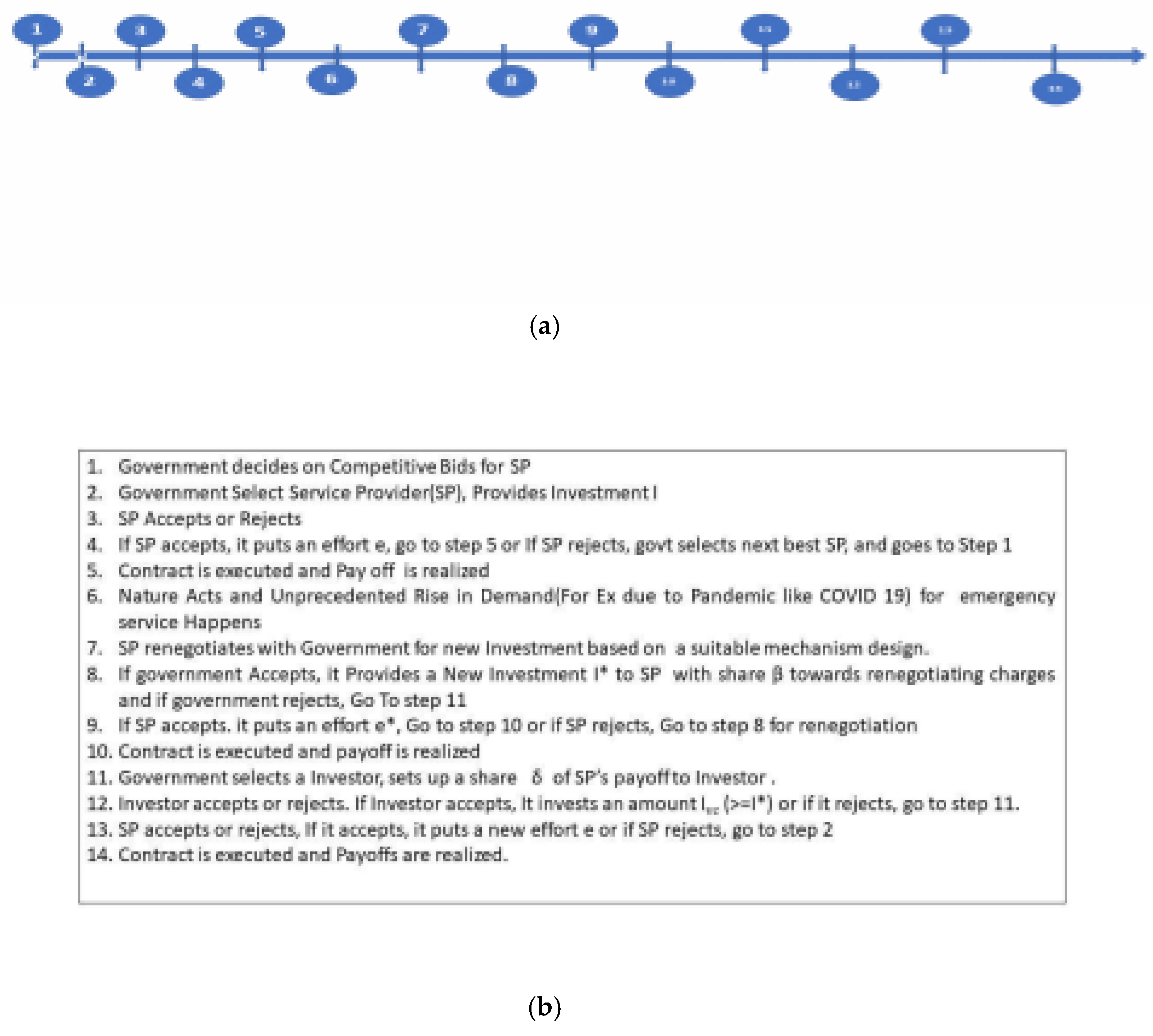
Our setting involves an EMS provider (SP) who is risk neutral and can be of two types (corporate/ non-profit) and is in a PPP contract with the central government, who is also a risk neutral player. The goal of SP and the government is to offer a high-quality, equitable emergency health service for the welfare of its citizens. A total of 3 scenarios occur in this principal (government)-agent (service provider) game. One of these scenarios involves another party, an investor who funds the SP when renegotiation efforts fail between the government and SP due to an unprecedented rise in demand. The timeline of the game is given below.
3.3. Timeline
- The timeline is given in 1(a) and 1(b) below.
3.4. Assumptions
• All the players are risk neutral. (It's easy to change the model to include risk averse players or a combination of risk-averse and risk neutral players).
• All the players emphasize equally service output as EMS is more humanitarian.
• If the Service Provider (SP) needs further funds and Investment, due to nature/change in demand, it can approach a VC firm with the help of the government.
• The government can take into account a target rate of Investment for post-contract investment v (Mason & Harrison, 2002).
VC takes into account a specific rate of return ω (Manigart et al, 2002). Effort e is observed only by social entrepreneurs / (Service Provider (SP)).
The agent operates in perfect competition and has a reservation utility
The government can monitor the benefits/outputs.
There are two types of effort, observable effort a and unobservable effort e which is given as below
z ≡ e + a
Unobservable effort e = two levels, where denotes effort at higher level and denotes effort at lower level is the probability for executing High Effort by the service provider who is risk neutral. We have assumed = 0.5 based on a binomial short rate model. ( Ho, T.S.Y & Lee, S.B. (2004) )
Effort is costly and follows the following quadratic equation:
a is contractible effort, e is not contractible but efficient non verifiable effort is cost effective. (Aghion & Rey, 2000)
• The tax rate is t and can change over time. In numerical, we have taken t as 20% (0.2) according to the current corporate taxes levied in India on corporations.
• The charge for emergency services by government is k= m*r. Here m has been taken as 3 according to a survey report by EMRI and Health Ministry of India (2012).
• The production function/Output function taken here is that of Cobb-Douglas Function having the form where α1 is the elasticity of effort and α2
is the elasticity of capital/ Investment. denotes the
efficiency. Value for Efficiency for Emergency Health Services (in India) =0.7 (Found by averaging
monthly efficiencies for all states for the year 2014 EMRI Report, 2014)
• Cost is quadratic function of demand elasticity (The values of a, b, c. In the current study undertaken, we have found a, b and c by regressing expenditures against demand elasticity for the years 2014, 2015, 2016, 2017, 2018.), a= 4652586, b=-8152965, c= 3620336)
• Production/ Output is a decreasing function of demand elasticity i.e. here we have taken it
as (Here exp = 2.718)
• In contractual situations which involve only government and service provider, π (I, 0) = π (0, e) = 0 i.e. payoff of SP becomes zero, SP does not provide any service if the government does not make any investment I or the SP does not exert any unobservable effort e.
• In contractual situations that involve the investor apart from government and service provider, we have π (I, 0, I ) π (Elitzur and Gavious, 2001). In other V C = (0, e, I ) V C = π (I, e, 0) = 0 words the payoff of SP becomes zero. Thus, SP does not provide any service if the government does not make any investment I or the investor does not make any investment I or the SP does not exert any effort e. V C
3.5. Strategic Decision Variables
e = Unobservable effort needed by the social entrepreneur i.e. SP, has two levels
I = Investment by the government
β = Share retained by social entrepreneur/ SP on renegotiation
= share retained by investor (VC) in the case renegotiation fails
IVC= Investment by the Investor (VC)
The base principal-agent model between government and service provider can be described as the following Principal-Agent (PA) problem: the objective function for the service provider i.e. the agent is given by
whereas the objective function of the government is given by
I
Subject to following constraints:
The first constraint is the incentive compatibility constraint
And
which is also known as the participation constraint.
The objective function has to be optimized with reference to effort. The values of e h and l decide whether the service provider has a probability to get into the action of moral hazard.
So in a PPP contract, when the service provider bids, he has to provide that optimal value of the effort that gives him the correct investment capital, and this is high effort. This is because the government assumes that the service provider is clean and moral hazard does not take place.
Further, any value higher than this optimal eh may not be practical because the government would select the lowest bidder and the service provider would not risk with higher effort levels as he could lose the contract.
Finally, there is a space and leverage for the service provider to put an effort lower than this effort to become more profitable, which needs not be shared with the government. The risk with which he can afford to do this is with a probability of 0.5. This leads to moral hazard.
Solving the above PA problem using the principle of backward induction, we solve agent's (SP’s) problem, first subject to the two constraints using the Karush Kuhn Tucker (KKT) conditions to obtain optimal and then substituting the value of in the Principal's unconstrained problem, we obtain the overall optimal conditions and solution for I and . Thus, we have, from the agent’s (service provider’s) problem:
Solving the Principal's i.e. , the government’s problem, which is an unconstrained optimization problem:
Applying the first order and second order conditions which indicate that the objective function is concave we have
Figure 3.
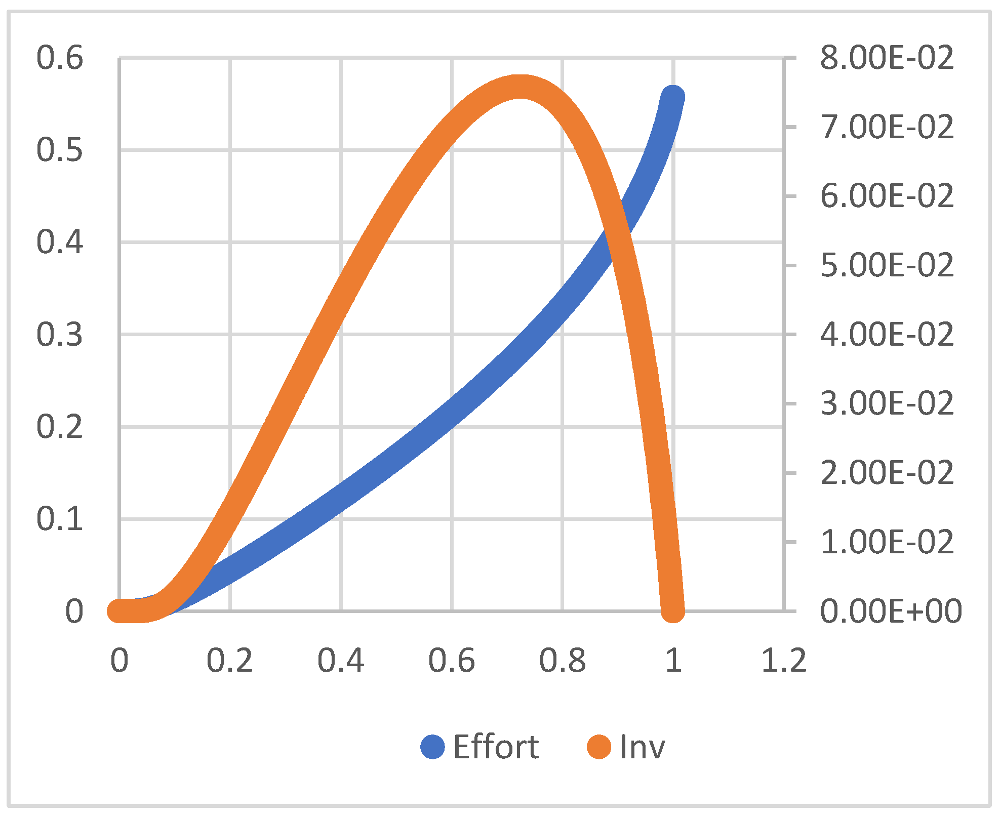
Figure 4.
Higher changes in effort or investment are required for changes in its respective elasticities, as shown from Figure 4. As demand for this scenario is assumed to be constant, the equilibrium lies at the intersection of the effort and investment curves. Following this, we arrive at the following propositions
Proposition 1
There are only two types of equilibria in this game for the given real situation:
- 1)
- e*= I*=0 at
- 2)
- (e*, I*) where e*>0, I*>0) at
Equilibrium 1 is the situation where there is no service. This is obvious since there will be no payoffs at this point.
Equilibrium 2 (Refer to Figure 2(b)) is the situation where the equilibrium investment by the government and the entrepreneur is positive, leading to a positive payoff to the service provider at the end of the contract. This is a situation which benefits both the service provider and the government in a PPP leading to a successful PPP contractual venture.
Proposition 2
For the second equilibrium when the service exists,
i.e. (e*, I*) where e*>0, I*>0) at
As
Despite the payoffs being positive, there is a possibility of opportunistic underinvestment by the government despite the high effort exerted by the service provider, leading to lower payoffs.
During situations where there is a rise in demand of services ( EMS), such as crisis situations like COVID 19, decreasing returns to scale may happen.( alpha + Beta >1), ( Effort put by SP will increase, despite not much rise in Investment). From literature(Labini, P.S., 1995.) we see that this may lead to change of Cobb Douglas Functions by a decreasing function multiplier. This indicates that by using this decreasing function multiplier (such as exponential function theta (used in this work, which is known as demand elasticity( (d1-d2)/d2) which can result in an Output ( Number of cases that are served using Capital investment provide by government specified before renegotiation ) that is needed by the PPP contract (Quality, access, equity, flexibility and efficiency) which has been specified during the contract when the situation was normal.(regular).
3.6. A COVID-19-Like Pandemic and Corporate Service Provider - Government Renegotiation
Let be the investment made during renegotiation. Then, the objective function for the service provider is given by
And the objective function of the government is given by
Subject to following constraints of the service provider
Solving the agent’s problem by applying the KKT conditions, we have
The proof of this is in Appendix 2.
Now, solving the principal's problem i.e. the government’s problem, which is an unconstrained optimization problem for the objective function.
Solving the first order with reference to , by back substituting the value of e
And then, solving the first order with reference to I, (Refer Appendix 2), we have
When we have
Where is substituted from prior equation.
For the objective function to be concave, we see that the first principal minor is negative and the second principal minor needs to be positive at the stationary point (optimal point). Also as
We have
And we also obtain all values of
From Figure 9, we see that as <=0.1, the plot of effort vs elasticity intersects at a point where
Which gives us the equilibrium conditions.
Following this, we arrive at the following propositions:
Proposition 3
There are two distinct equilibrium conditions in the current scenario.
They are
The first is an equilibrium point when I>0, e>0 and the payoffs are positive for both the SP and the government. The second is a set of equilibrium points where the firm ceases to exist, as both I=0 and e=0 for this set of points, as seen from Figure 3.
Proposition 4
In equilibrium conditions under the current scenario, the payoffs would not be lower, as both the players, government and service provider may tend to exhibit opportunistic behavior, unless there is risk of terminating the service.
6.5. A COVID 19-Like Pandemic when an Investor Funds the Corporate Service Providers
The Agent's Problem i.e. the service provider’s problem becomes
ST
The KKT conditions are
Solving in similar way to the previous situations
The investor's problem is as follows:
Substituting in above unconstrained optimization problem, we have the above set of equations as
Solving, we have
If the investor turns down the reinvestment due to the low returns, then and .
Furthermore, we see that the objective function is concave as the double differential is negative.
For the Government Problem, the objective function becomes
Substituting from the previous equations in the above equations and simplifying it we have the equation simplifying to the following form
Where is a constant not affecting the optimal decision variable.
As this is an unconstrained optimization problem and as the second differential of the objective function is negative, the function is concave.
The above unconstrained optimization problem leads to the following optimal solution:
As , we have , for which the concavity conditions are satisfied.
Figure 10.
Plot of Effort and IVC vs Elasticity.
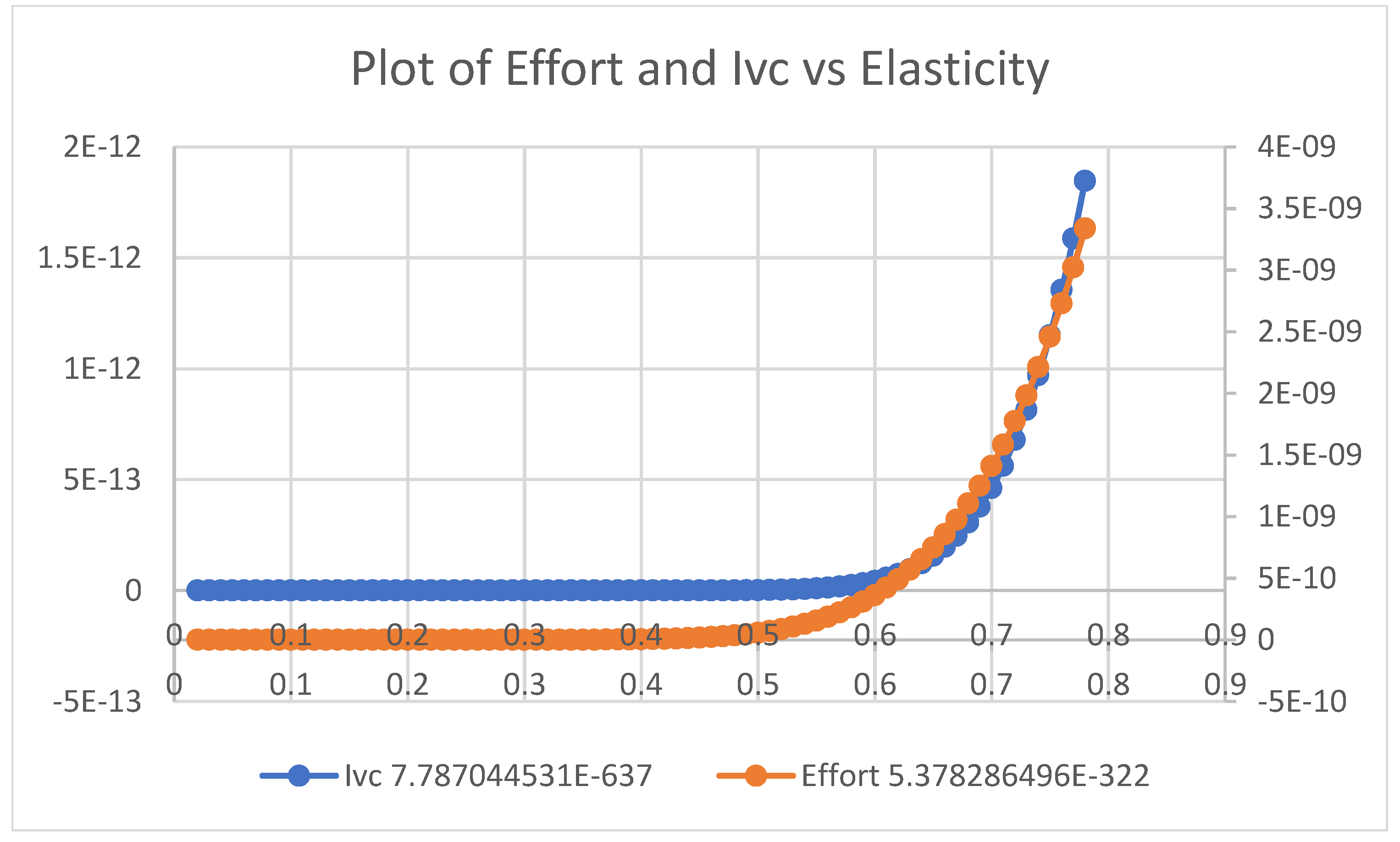
Figure 11.
Plot of Equilibrium Diagram: Series1= Effort, Series 2= Ivc.
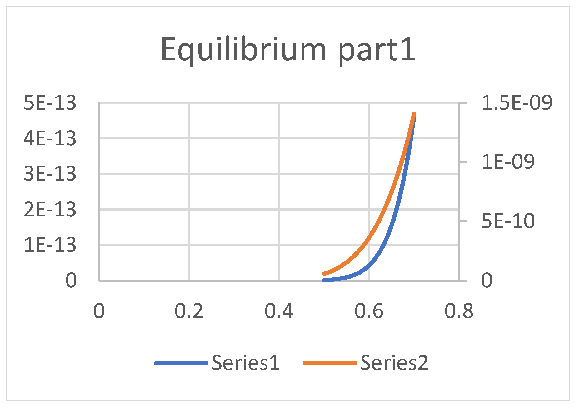
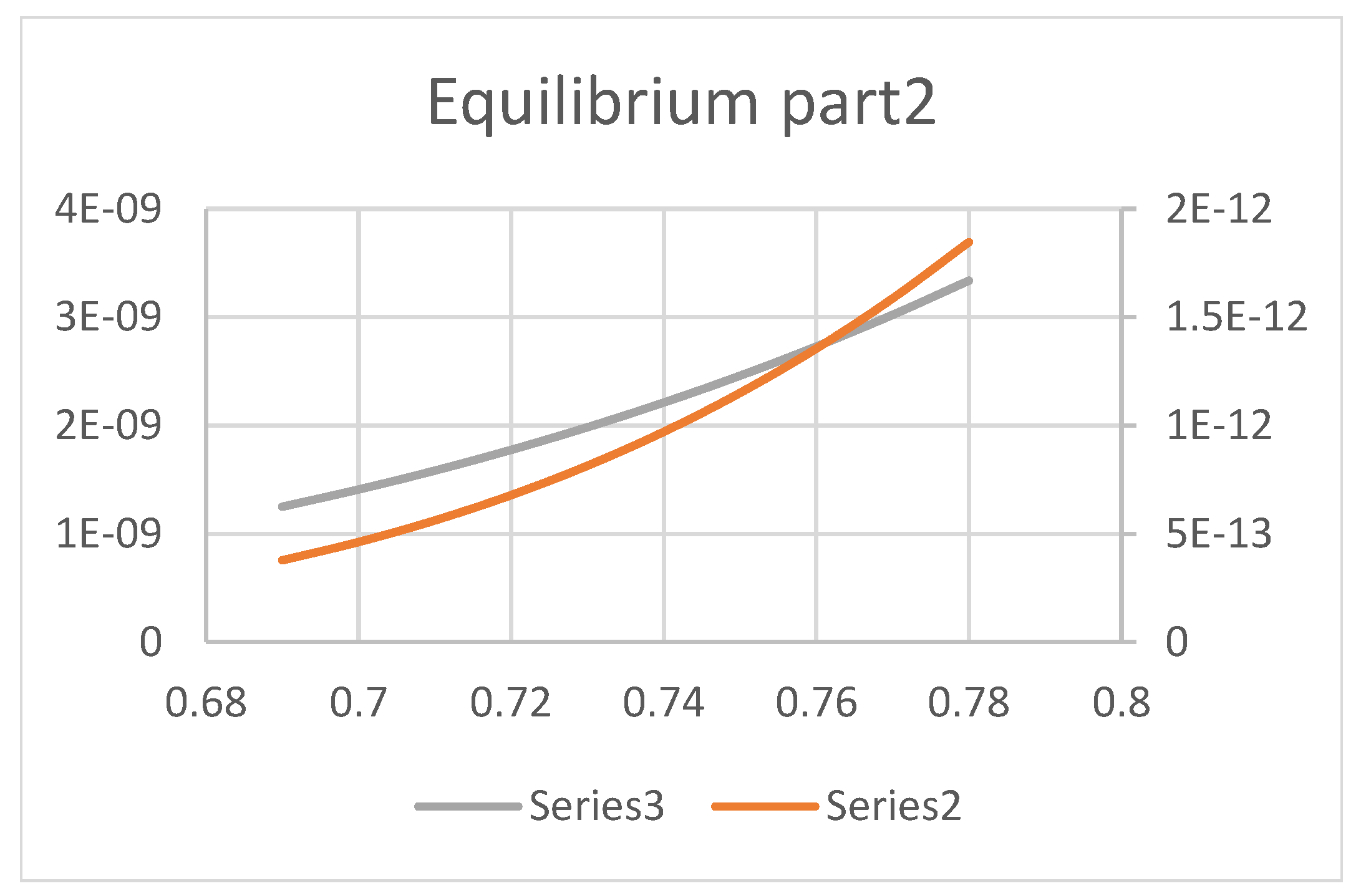
Figure 12.
Plot of Equilibrium Diagram Series2 = Ivc, Series3= Effort.
Based on the above figures, we arrive at the following propositions:
Proposition 5
There are two equilibrium conditions for which Ivc > 0 and e > 0, as shown in Figure 4.
- 1)
- The first equilibrium occurs at
- 2)
- The second equilibrium occurs at
At these equilibrium points, we see with increase in elasticities, effort increases whereas investment decreases and both these equilibrium conditions provide positive payoffs to the service provider, investor and the government.
The results for corporate service providers is summarized in Table 1.
4. Results and Discussion
4.1. Scenario 1
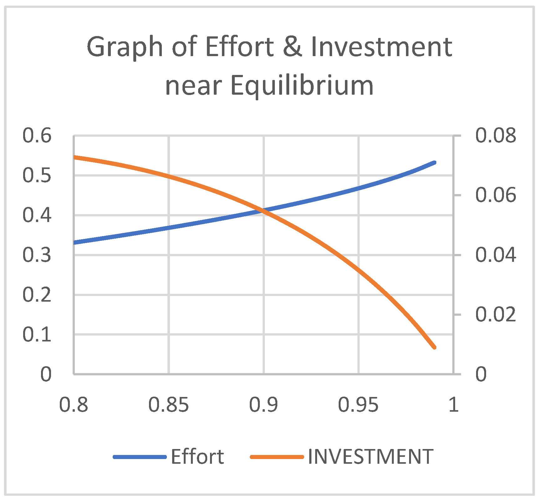
The equilibrium for the first scenario is obtained at
We have used the following principle for obtaining the general equilibrium. Because emergency health services demand depends more on the labor put in by the service provider, the graph shows that effort increases in its elasticity, which implies an increase in demand of service, as also indicated in section 4. Further, we see that the investment initially rises and then falls with a decrease in its elasticity, which again implies that investment increases and decreases with decrease in demand. But in the current scenario, as the demand is assumed to be constant, we can safely conclude that the equilibrium should lie at an intersection of the effort and investment curves. As previously shown, this occurs at
From Figure 13 and Figure 14 above, we see that there is a negative relationship between the effort and capital investment around the equilibrium point, which indicates that the elasticity of substitution for the given scenario is negative, providing the insight that labor and investment complement each other. Thus, we can infer that if the demand of the service to be provided increases, there needs to be an increase in the government’s investment, leading to an increase in the effort of the service provider, thereby improving citizens’ welfare.
4.2. Scenario 2
The plot between payoff of the Service Provider and effort,as shown in Figure 18 below, is concave and increasing, indicating that demand would be met, and as well implying that the output quality would be better when the effort is put on a more consistent basis than a fluctuating basis.
Further, as shown in Figure 19, increased investment by the government when the demand changes leads to an increased effort by the service provider. Furthermore, since the curve is increasing and convex, we see that marginal effort increases with reference to investment and fluctuating efforts are bound to happen despite increases in the investment.
Figure 20 plots the service provider’s and government’s payoff functions vs elasticity and shows that equilibrium where the service can be provided occurs closer to Also, Figure 20 and Figure 21 demonstrate that the payoffs of the government and the service provider are positive in the above-mentioned region of elasticities, showing a linear increasing relationship.
Plotting the payoff of government and the investment by government after renegotiation shows a linear increasing relationship unlike scenario 1, where government payoff decreased with increase in its investment, indicating that the government would be more willing for renegotiating the contract with the service provider in the case of an unprecedented raise in demand.
4.3. Scenario 3
The plot of (The percentage share of service provider's payoff to the investor), which is determined by government, is shown in the Figure 23. Accordingly, the maximum share that an investor can obtain is 18% of the service provider's payoff excluding the taxes. Further, we see that it increases with increase in effort, which increases the service provider's payoff.
Figure 24 demonstrates that effort must be exerted consistently without much fluctuation with an increase in investment and higher demand, as the curve is increasing and concave. The investor’s payoff is positive and increasing in the service provider's payoff in a linear fashion, as shown in Figure 25, indicating that the investment made by theory investor provides him with positive returns, as shown in the increasing linear relationship in Figure 26.
Figure 27 plots the investor’s and service provider’s payoffs. As discussed earlier, both have an increasing linear relationship with investment made by the VC.
The payoff of the service provider is an increasing concave function in effort, indicating that fluctuations in payoff are bound to happen rather than being consistent, as shown in Figure 28.
5. Conclusions and Managerial Insights
The government’s decision on forming a PPP to provide emergency medical services varies on the effort that can be exerted by the service provider in three different situations that the government faces for providing welfare to its citizens. From the above results we see that the service provider exerts an effort in direct proportion to the capital invested by the government, in situations where there is a demand change i.e. say during a pandemic, than in a normal situation. This leads to government’s underinvestment during such situation despite lower payoffs, as it can expect higher effort exerted by the service provider, leading to better service to the patients. Further, in situations where there is an unprecedented change in demand, there are opportunities for moral hazard to occur, so the government needs to monitor the capital investment that it provides to the service providers. Also, we see that the payoff of the government increases with the service provider’s payoff in all the situations, though from the observations, we can infer that in situations 2 and 3, the payoffs are much lower. This can be attributed to the fact that incase of unprecedented rise in demand, the service provider exerts more effort which increases the costs leading to a decrease of their payoff. Further in a situation, where the investor funds the service provider, the government needs to focus on selecting an investor who gives the service provider an opportunity for maximizing their payoffs even in the face of a humanitarian situation like COVID 19. This can be inferred from the results shown in graphs 15, 22 and 24 which provide the insight that the investor’s returns do not provide the government the payoffs that it would have obtained without the involvement of the investor.
References
- Agheon, P., Holmstrom, B., & Tirole, J. (2000). Agency costs, firm behavior and the nature of competition. Mimeo.
- Akintoye, A., & Kumaraswamy, M. (2004). TG72: Public-private partnership. Research roadmap—Report for consultation (CIB Publication No. 406). International Council for Research and Innovation in Building and Construction. http://www.cibworld.nl.
- Alonso-Conde, A. B., Brown, C., & Rojo-Suarez, J. (2007). Public-private partnerships: Incentives, risk transfer, and real options. Review of Financial Economics, 16(4), 335–349. [CrossRef]
- Auriol, E., & Picard, P. M. (2013). A theory of BOT concession contracts. Journal of Economic Behavior & Organization, 89, 187–209.
- Bennett, S., & Mills, A. (n.d.). Government capacity to contract: Health sector experience and lessons. https://onlinelibrary.wiley.com/doi/pdf/10.1002/(SICI)1099-162X(1998100)18:4%3C307::AID-PAD24%3E3.0.CO;2-D.
- Bergman, B. (1990). Public policy in a principal-agent framework [PDF file]. (Retrieved April 2, 2019).
- Besley, T., & Ghatak, M. (2017). Public-private partnerships for the provision of public goods: Theory and an application to NGOs. Research in Economics, 71(2), 356–371. [CrossRef]
- Bettignies, J.-E. de, & Ross, T. W. (2004). The economics of public-private partnerships. Canadian Public Policy, 30(2), 135–154. https://ideas.repec.org/a/cpp/issued/v30y2004i2p135-154.html.
- Blanken, A., & Dewulf, G. (2009). PPPs in health: Static or dynamic? The Australian Journal of Public Administration, 69(S1), 35–47. [CrossRef]
- Buso, M. (2019). Bundling versus unbundling: Asymmetric information on information externalities. Journal of Economics, 128(1), 1–25.
- Carr, B. G., Caplan, J. M., Pryor, J. P., & Branas, C. C. (2006). A meta-analysis of prehospital care times for trauma. Prehospital Emergency Care, 10(2), 198–206. [CrossRef]
- Casady, C. B., Eriksson, K., Levitt, R. E., & Scott, W. R. (2020). (Re)defining public-private partnerships (PPPs) in the new public governance (NPG) paradigm: An institutional maturity perspective. Public Management Review, 22(2), 161–183.
- Chou, J.-S., Ping Tserng, H., Lin, C., & Yeh, C.-P. (2012). Critical factors and risk allocation for PPP policy: Comparison between HSR and general infrastructure projects. Transport Policy, 22, 36–48. [CrossRef]
- Chung, C. (2001). The evolution of emergency medicine. Hong Kong Journal of Emergency Medicine, 8(2), 84–89. [CrossRef]
- Cooley, T. F., & Smith, B. D. (1987). Equilibrium in cooperative games of policy formulation (Working Paper No. 84). Rochester Centre of Economic Research.
- David, S. S., Vasnaik, M., & TV, R. (2007). Emergency medicine in India: Why are we unable to walk the talk? Emergency Medicine Australasia, 19(4), 289–295. [CrossRef]
- Baxter, D., & Casady, C. B. (2020). Proactive and strategic healthcare public-private partnerships (PPPs) in the coronavirus (COVID-19) epoch. Unpublished manuscript.
- De Brux, J. (2010). The dark and bright sides of renegotiation: An application to transport concession contracts. Utilities Policy, 18(2), 77–85. [CrossRef]
- Asian Development Bank. (n.d.). Improving health and education service delivery in India through public-private partnerships. https://www.adb.org.
- Dykstra, E. H. (1997). International models for the practice of emergency care. The American Journal of Emergency Medicine, 15(2), 208–209. [CrossRef]
- Elitzur, R., & Gavious, A. (2003). Contracting, signaling, and moral hazard: A model of entrepreneurs, 'angels,' and venture capitalists. Journal of Business Venturing, 18(6), 709–725. [CrossRef]
- Elitzur, R., & Gavious, A. (2011). Selection of entrepreneurs in the venture capital industry: An asymptotic analysis. European Journal of Operational Research, 215(2), 705–713. [CrossRef]
- National Health Systems Resource Centre (NHSRC). (n.d.). Emergency medical service (EMS) in India: A concept paper. https://www.nhsrcindia.org.
- Heartfile. (n.d.). Good governance and partnerships for health. http://heartfile.org.
- Gregory, A. W., & Hansen, B. E. (1996). Residual-based tests for cointegration in models with regime shifts. Journal of Econometrics, 70(1), 99–126. [CrossRef]
- Grimsey, D., & Lewis, M. (2007). Public-private partnerships and public procurement. Agenda: A Journal of Policy Analysis and Reform, 14(2), 171–188.
- Gupta, M. D., & Rani, M. (2004). India's public health system: How well does it function at the national level? (Policy Research Working Paper No. 3447). The World Bank. [CrossRef]
- Hart, O. (2003). Incomplete contracts and public ownership: Remarks, and an application to public-private partnerships. The Economic Journal, 113(486), C69–C76. [CrossRef]
- Hayllar, M. R., & Wettenhall, R. (2009). Public-private partnerships: Promises, politics, and pitfalls. The Australian Journal of Public Administration, 69(S1), 1–7. [CrossRef]
- Ho, S. P. (2009). Government policy on PPP financial issues: Bid compensation and financial renegotiation. In E. R. Yescombe (Ed.), Policy, finance & management for public-private partnerships (pp. 267–300). Wiley. [CrossRef]
- Ho, T. S. Y., & Lee, S. B. (2004). The Oxford guide to financial modelling: Applications for capital markets, corporate finance, risk management and financial institutions. Oxford University Press.
- Xing, H., Li, Y., & Li, H. (2020). Renegotiation strategy of public-private partnership projects with asymmetric information—An evolutionary game approach. Sustainability, 12(10), 4172.
- Hung, K. K. C., Cheung, C. S. K., Rainer, T. H., & Graham, C. A. (2009). International EMS systems: China. Resuscitation, 80, 732–735.
- Kennedy, G. M. (2013). Can game theory be used to address PPP renegotiations? A retrospective study of the Metronet–London Underground PPP (Master’s thesis, University of London).
- Klijn, E. H., & Koppenjan, J. (2016). The impact of contract characteristics on the performance of public-private partnerships (PPPs). Public Money & Management, 36(6), 455–462. [CrossRef]
- KPMG. (2015). The emerging role of PPP in Indian healthcare sector. India Brand Equity Foundation. https://www.ibef.org/download/PolicyPaper.pdf.
- Liu, X., Hotchkiss, D. R., & Bose, S. (2007). The impact of contracting-out on health system performance: A conceptual framework. Health Policy, 82, 200–211. [CrossRef]
- Lv, J., Ye, G., Liu, W., Shen, L., & Wang, H. (2015). Alternative model for determining the optimal concession period in managing BOT transportation projects. Journal of Management in Engineering, 31(4), 04014066. [CrossRef]
- Balarajan, Y., Selvaraj, S., & Subramanian, S. V. (2011). Public-private partnerships in health services in India: Boundaries blurred. Economic and Political Weekly, 46(4), 62–71.
- Macal, C. M., & North, M. J. (2010). Tutorial on agent-based modeling and simulation. Journal of Simulation, 4(3), 151–162. [CrossRef]
- Manigart, S., De Waele, K., Wright, M., Robbie, K., Desbrières, P., Sapienza, H. J., & Beekman, A. (2002). Determinants of required return in venture capital investments: A five-country study. Journal of Business Venturing, 17(4), 291–312. [CrossRef]
- Mason, C. M., & Harrison, R. T. (2002). Is it worth it? The rates of return from informal venture capital investments. Journal of Business Venturing, 17(3), 211–236. [CrossRef]
- Medda, F. R., Carbonaro, G., & Davis, S. L. (2013). Public-private partnerships in transportation: Some insights from the European experience. IATSS Research, 36(2), 83–87. [CrossRef]
- Ministry of Health and Family Welfare. (n.d.). Stabilizing the emergency medical services in India. https://a2hp.mohfw.gov.in/ResourceDocuments/STABILIZING THE EMERGENCY MEDICAL SERVICE INDIA.pdf.
- Mitroff, I. I., & Mason, R. O. (1981). The metaphysics of policy and planning: A reply to Cosier. Academy of Management Review, 6(4), 649–651. [CrossRef]
- Oliveira Cruz, C., & Cunha Marques, R. (2014). Theoretical considerations on quantitative PPP viability analysis. Journal of Management in Engineering, 30(1), 04014017. [CrossRef]
- Prakash, G., & Singh, A. (n.d.). A new public management perspective in Indian e-governance initiatives. https://unpan1.un.org/intradoc/groups/public/documents/UN-DPADM/UNPAN040636.pdf.
- Baru, R., & Nundy, M. (2008). Private-public partnerships: Boundaries blurring in health services in India. Economic and Political Weekly, 43(4), 62–71.
- Raman, A. V., Björkman, J. W., & Björkman, J. W. (2008). Public-private partnerships in health care in India. Routledge. [CrossRef]
- Roberts, M. J., Hsiao, W., Berman, P., & Reich, M. R. (n.d.). Getting health reform right: A guide to improving performance and equity. http://www.ssu.ac.ir/fileadmin/templates/fa/daneshkadaha/daneshkade-behdasht/manager_group/upload_manager_group/manabe_elmi/e-book/english/edalat_dar_nezame_salamat/2.Getting_Health_Reform_Right.pdf.
- Ross, T. W., & Yan, J. (2015). Comparing public-private partnerships and traditional public procurement: Efficiency vs. flexibility. Journal of Comparative Policy Analysis: Research and Practice, 17(5), 448–466. [CrossRef]
- Schneider, S. M., Gardner, A. F., Weiss, L. D., Wood, J. P., Ybarra, M., Beck, D. M., & Jouriles, N. J. (2010). The future of emergency medicine. The Journal of Emergency Medicine, 39(2), 210–215. [CrossRef]
- Serra, D., Serneels, P., & Barr, A. (n.d.). Intrinsic motivations and the non-profit health sector: Evidence from Ethiopia. http://hdl.handle.net/10419/36127.
- Shi, L., Zhang, L., Onishi, M., Kobayashi, K., & Dai, D. (2018). Contractual efficiency of PPP infrastructure projects: An incomplete contract model. Mathematical Problems in Engineering, 2018, 1–13. [CrossRef]
- Singh, A., & Prakash, G. (2010). Public-private partnerships in health services delivery. Public Management Review, 12(6), 829–856. [CrossRef]
- Subhan, I., & Jain, A. (2010). Emergency care in India: The building blocks. International Journal of Emergency Medicine, 3(4), 207–211. [CrossRef]
- Titoria, R., & Mohandas, A. (2019). A glance on public-private partnership: An opportunity for developing nations to achieve universal health coverage. International Journal of Community Medicine and Public Health, 6(3), 1353–1357. [CrossRef]
- Tserng, H. P., Russell, J. S., Hsu, C. W., & Lin, C. (2012). Analyzing the role of national PPP units in promoting PPPs: Using new institutional economics and a case study. Journal of Construction Engineering and Management, 138(2), 242–249.
- Ho, T. S. Y., & Lee, S. B. (2004). The Oxford guide to financial modelling: Applications for capital markets, corporate finance, risk management and financial institutions. Oxford University Press.
- Vasudevan, V., Singh, P., & Basu, S. (2016). Importance of awareness in improving performance of emergency medical services (EMS) systems in enhancing traffic safety: A lesson from India. Traffic Injury Prevention, 17(7), 699–704. [CrossRef]
- Wibowo, A., & Alfen, H. W. (2015a). Critical success factors in public-private partnership (PPP) on infrastructure delivery in Nigeria. Built Environment Project and Asset Management, 5(1), 212–225. [CrossRef]
- Wibowo, A., & Alfen, H. W. (2015b). Government-led critical success factors in PPP infrastructure development. Built Environment Project and Asset Management, 5(1), 121–134. [CrossRef]
Figure 9.
Plot of Investment vs Effort (Scenario 2).
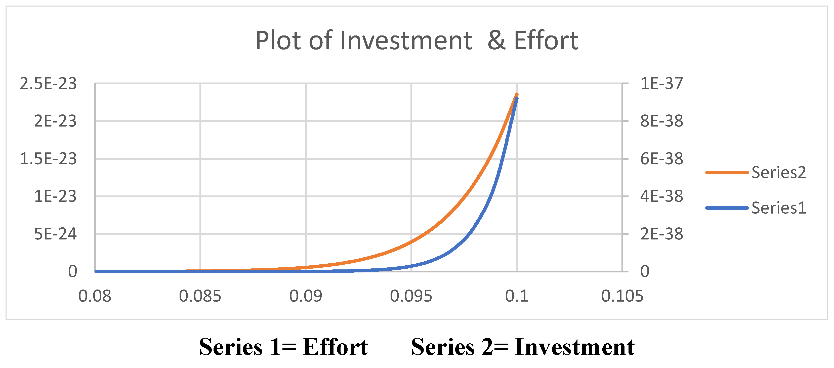
Figure 13.
Plot of Effort vs Investment.
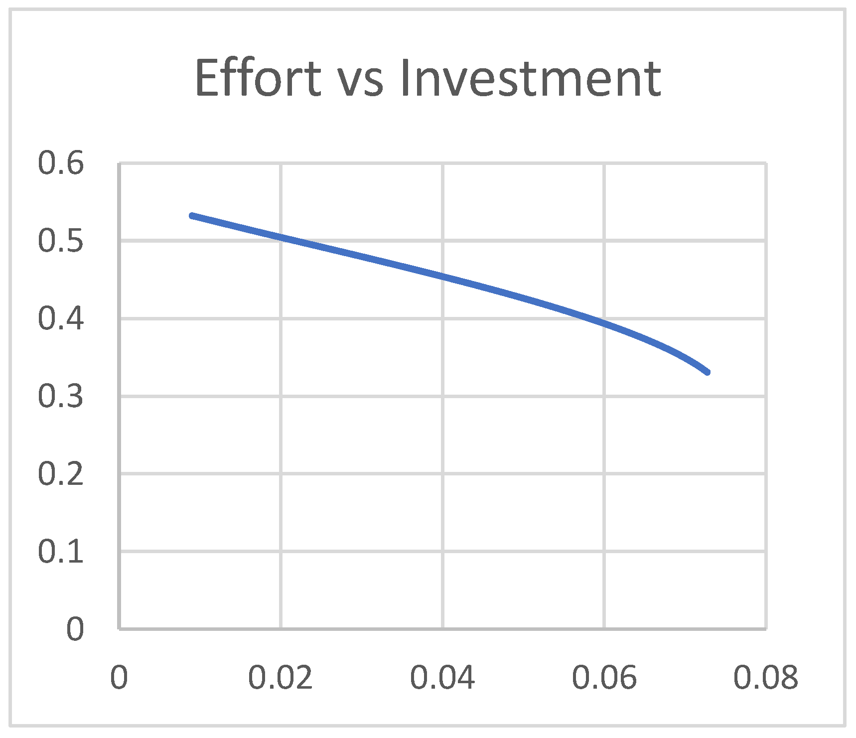
Figure 14.
Plot of SP payoff, Govt. Payoff vs Investment.
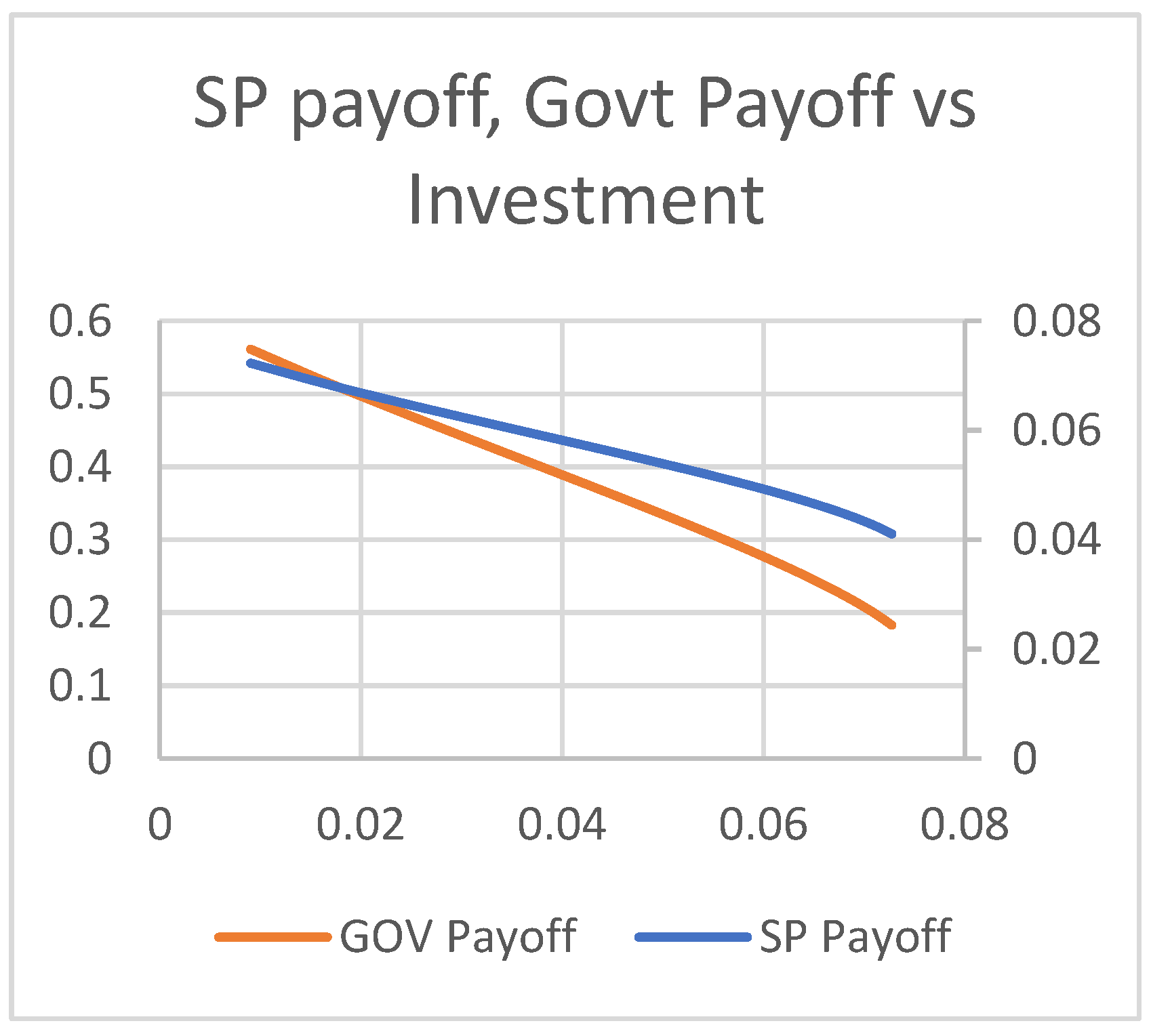
Figure 15.
Plot of Gov. Payoff vs SP Payoff.
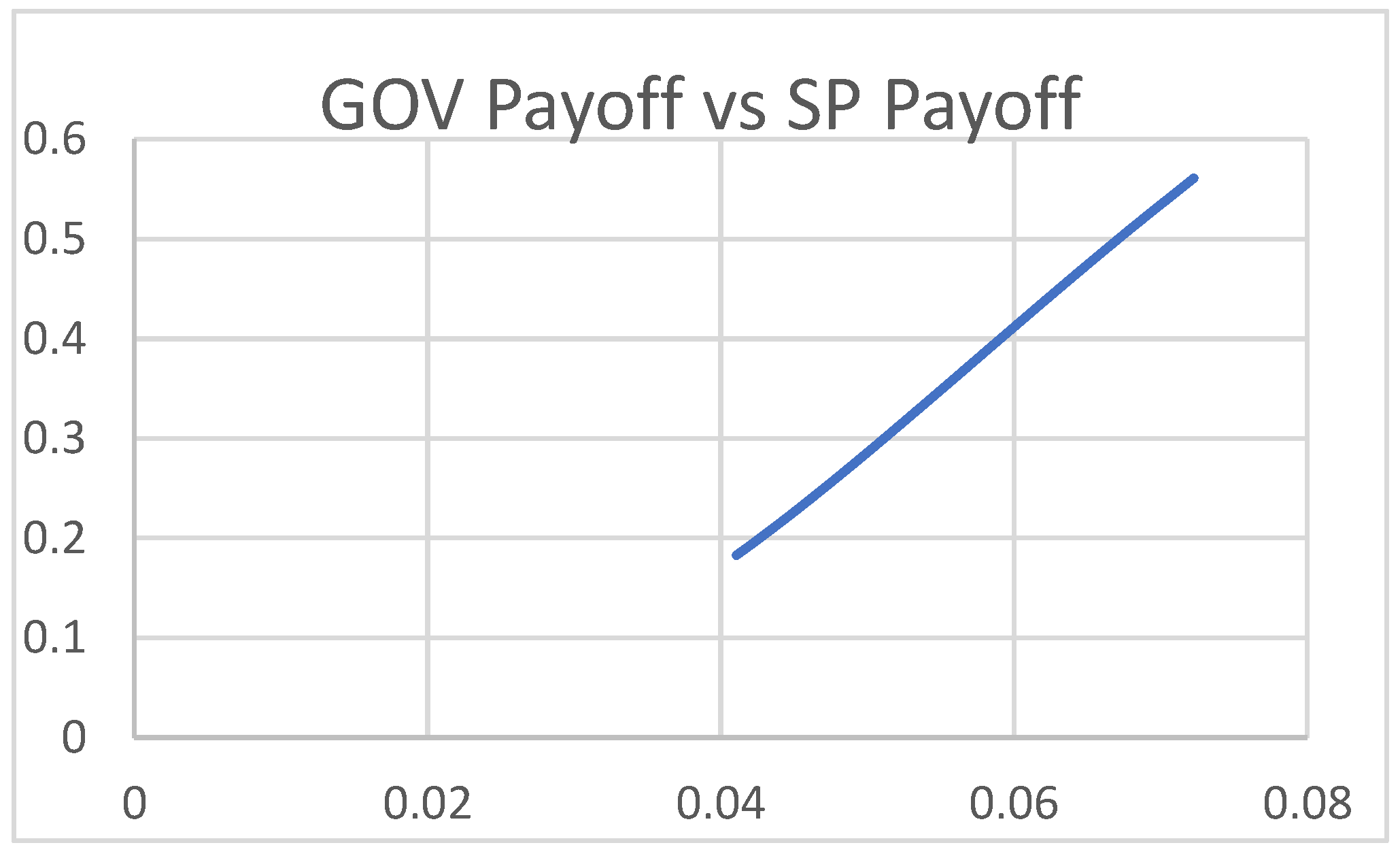
Figure 16.
Plot of SP Payoff vs Effort.
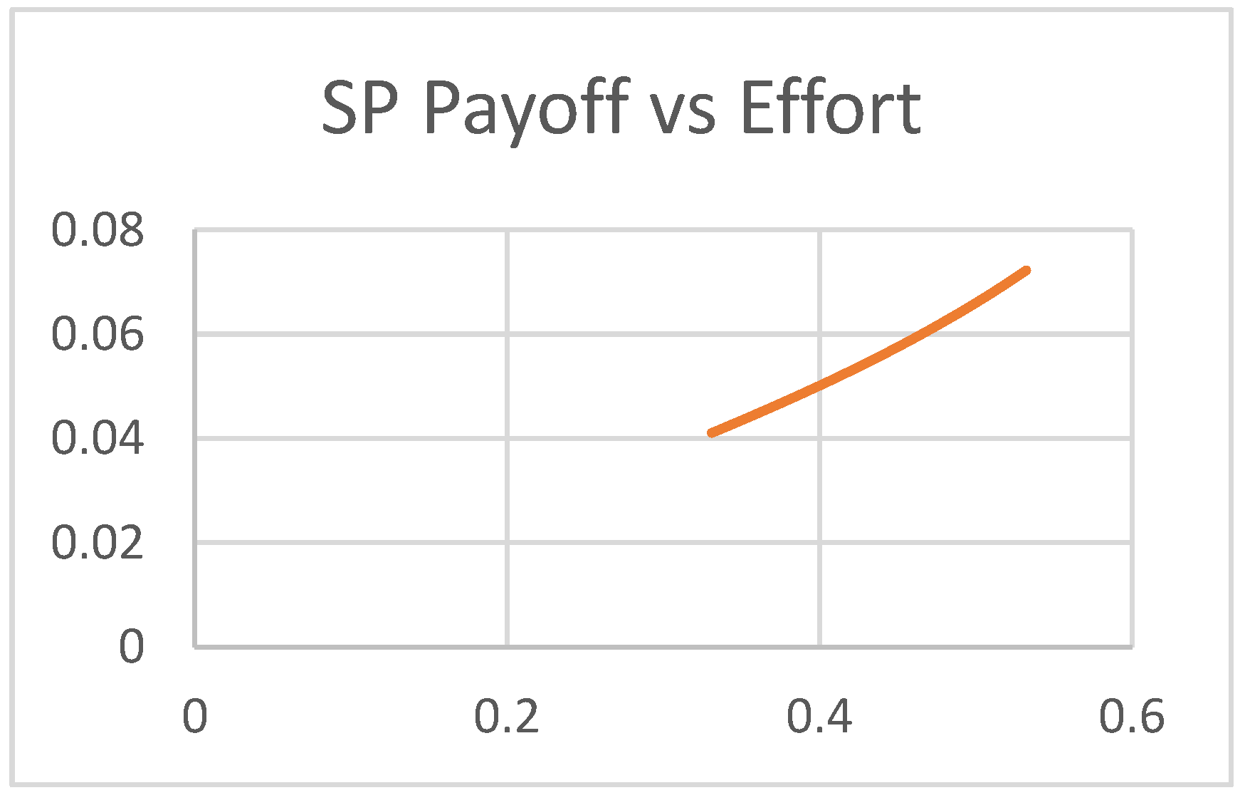
Figure 17.
Plot of SP Payoff, Govt. Payoff vs Effort.
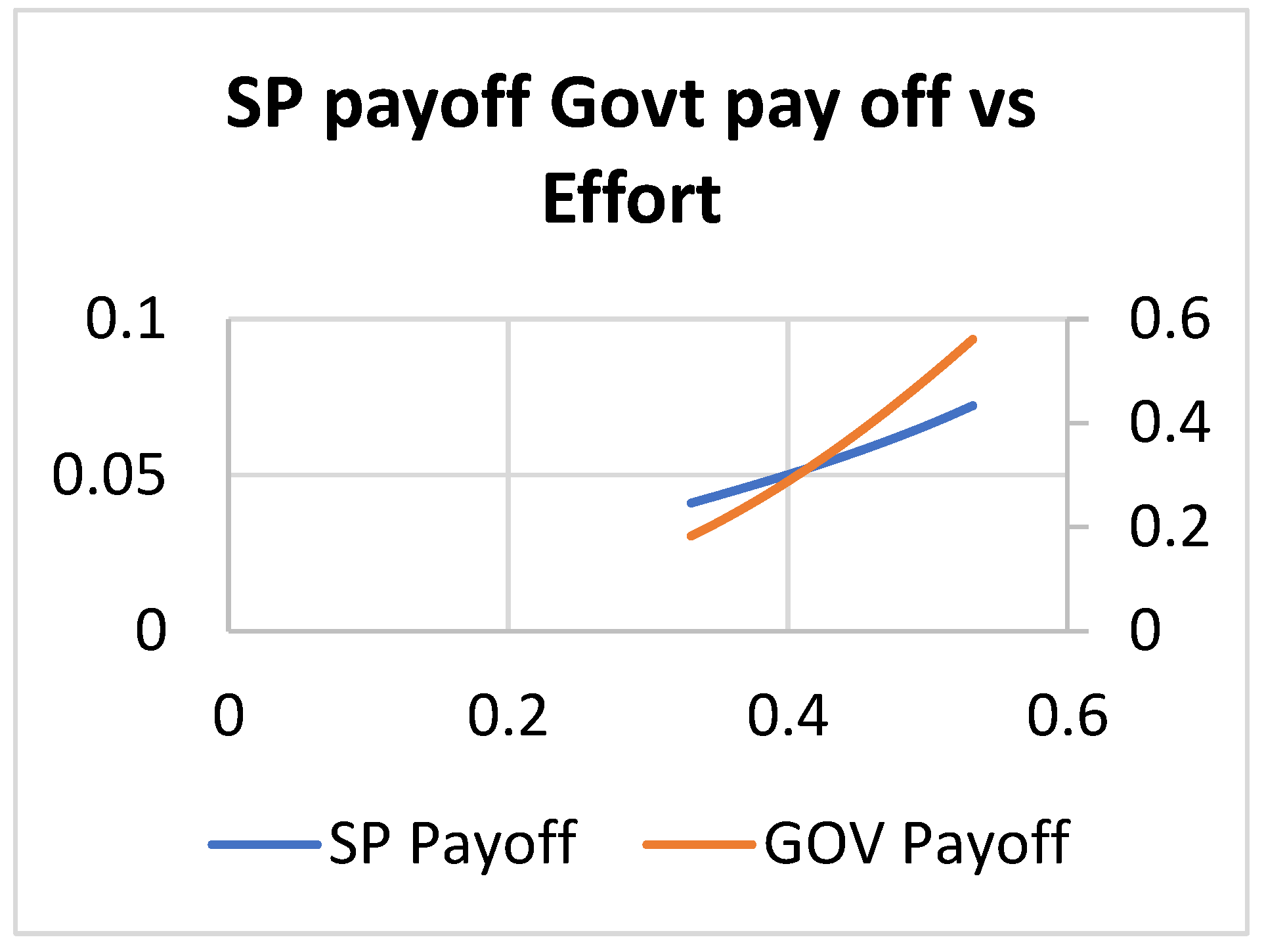
Figure 18.
Plot of SP Payoff vs Effort.
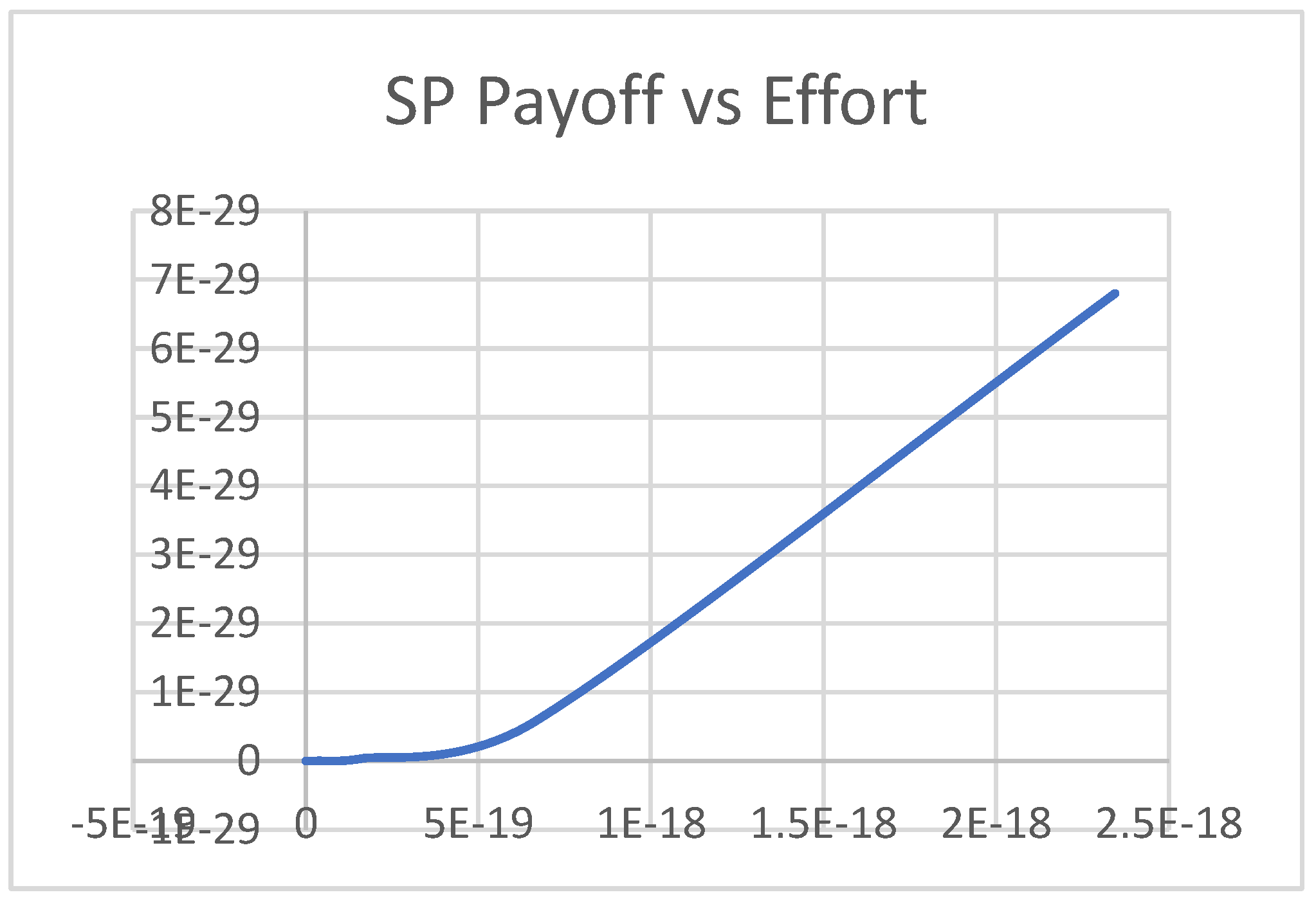
Figure 19.
Plot of Effort vs Investment.
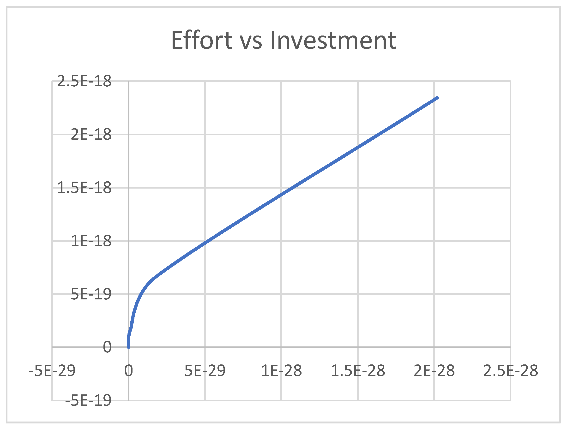
Figure 20.
Plot of Payoff Functions.
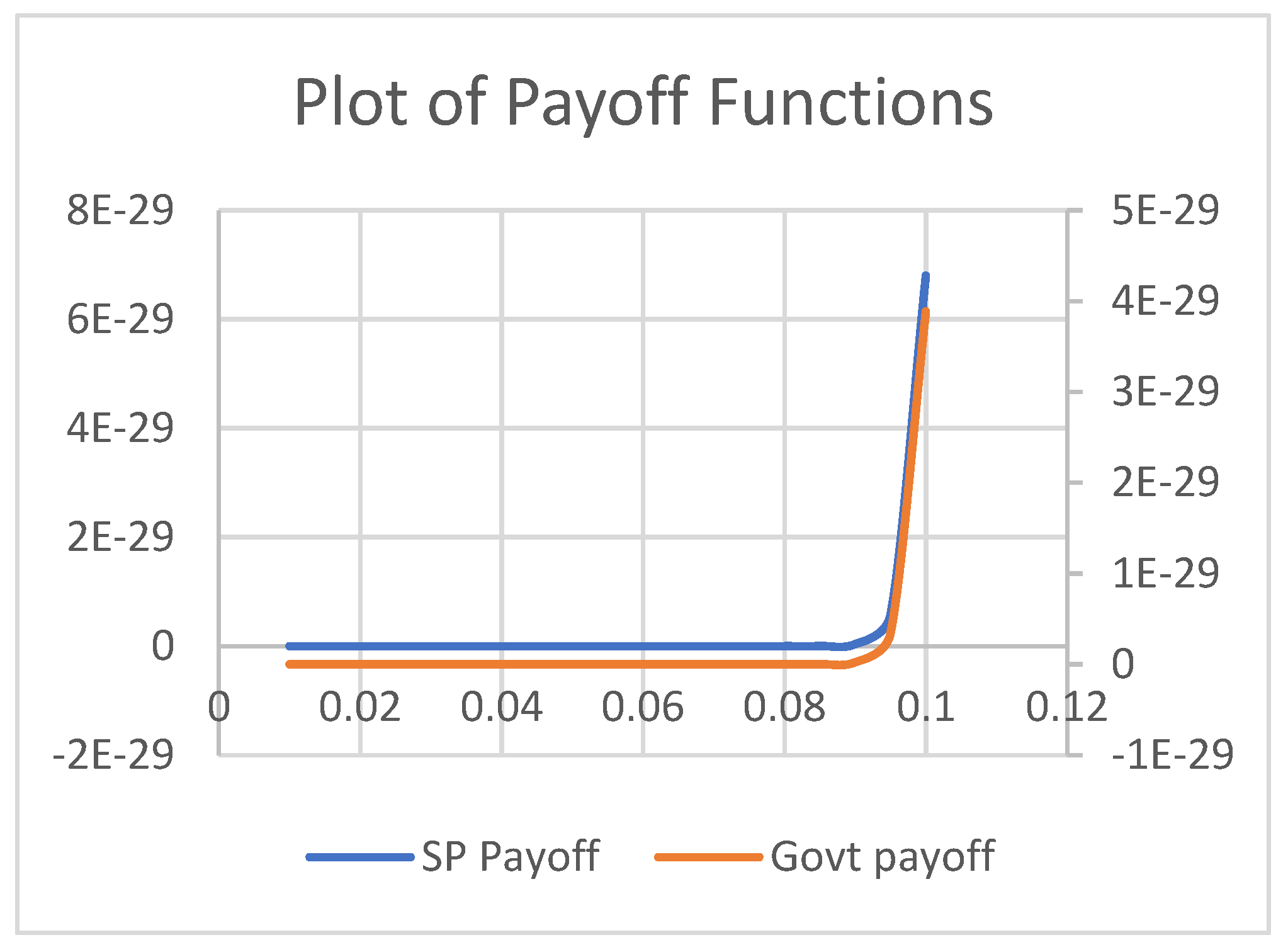
Figure 21.
Plot of Govt. Payoff vs SP Payoff.
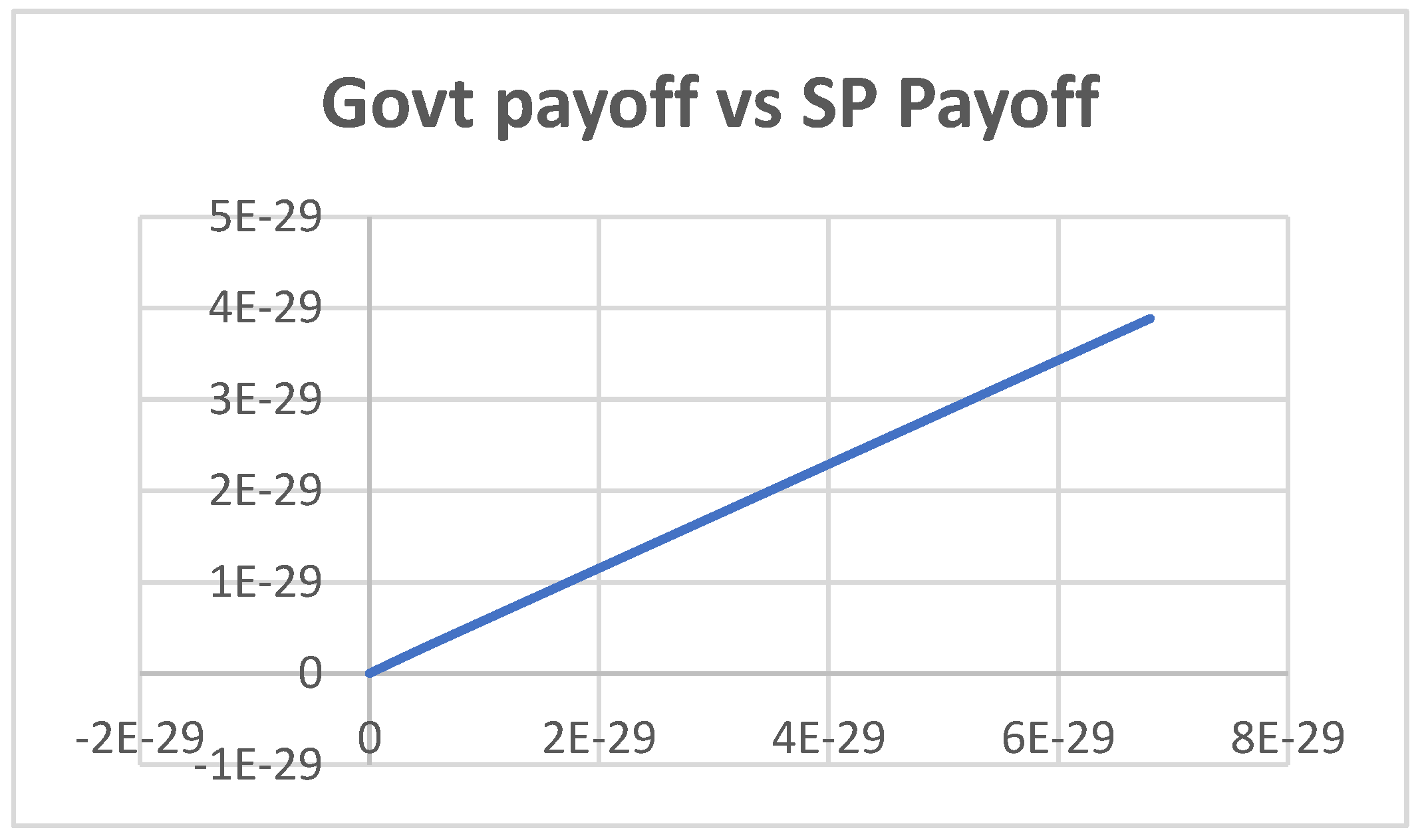
Figure 22.
Plot of Govt. Payoff vs Investment.
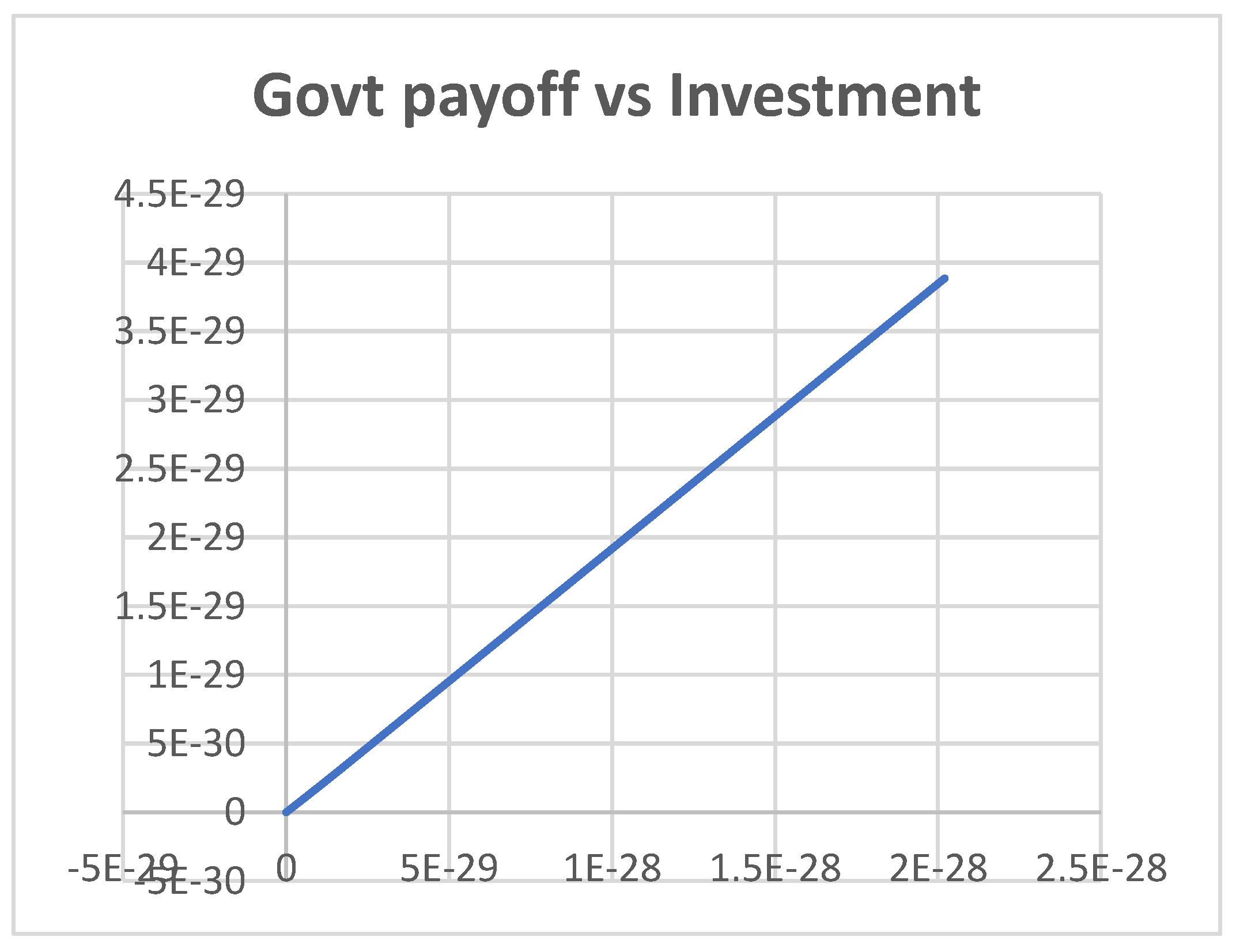
Figure 23.
Plot of Percentage share vs Elasticity.
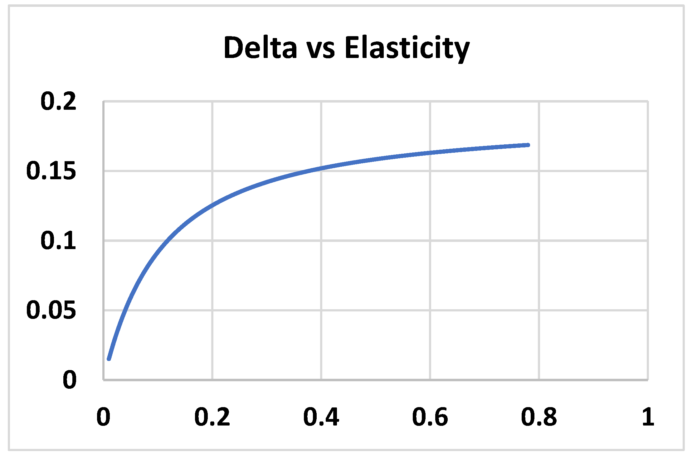
Figure 24.
Plot of Effort vs Investment.
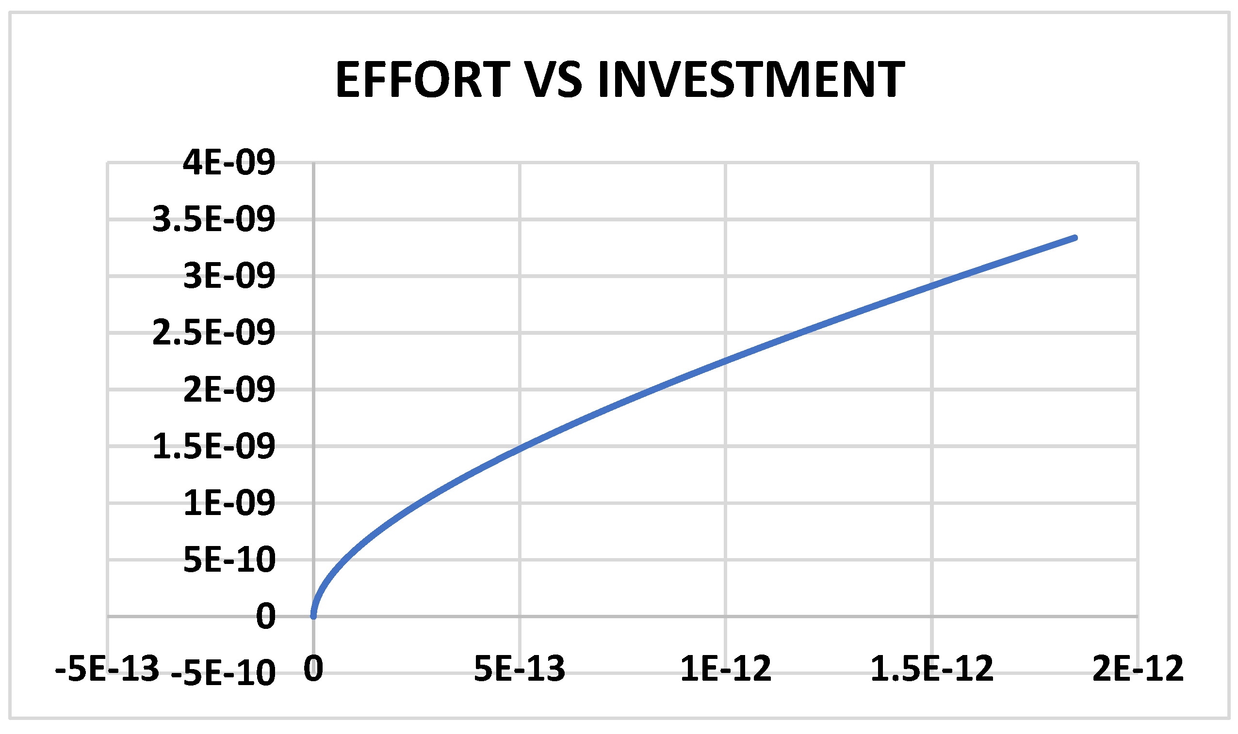
Figure 25.
Plot of Investor Payoff vs SP Payoff.
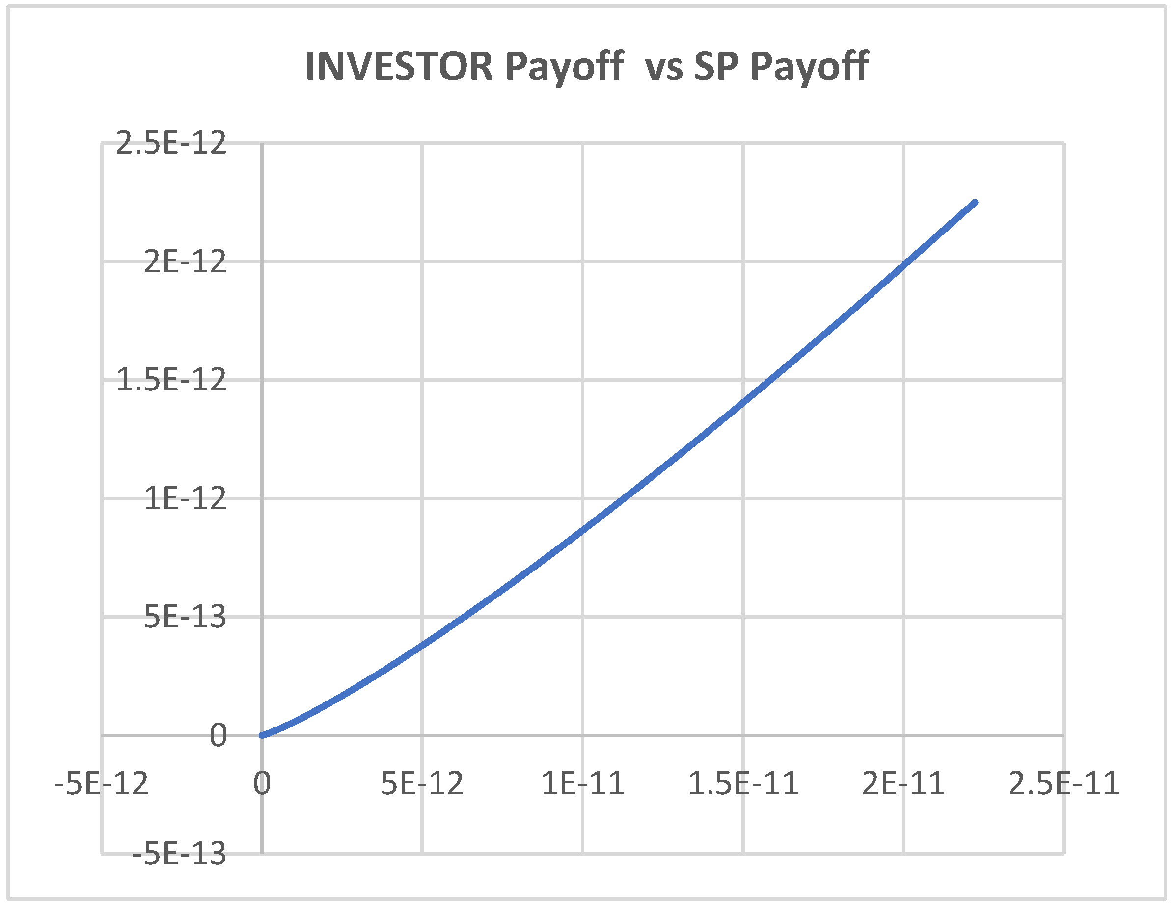
Figure 26.
Plot of Investment Payoff vs Investment.
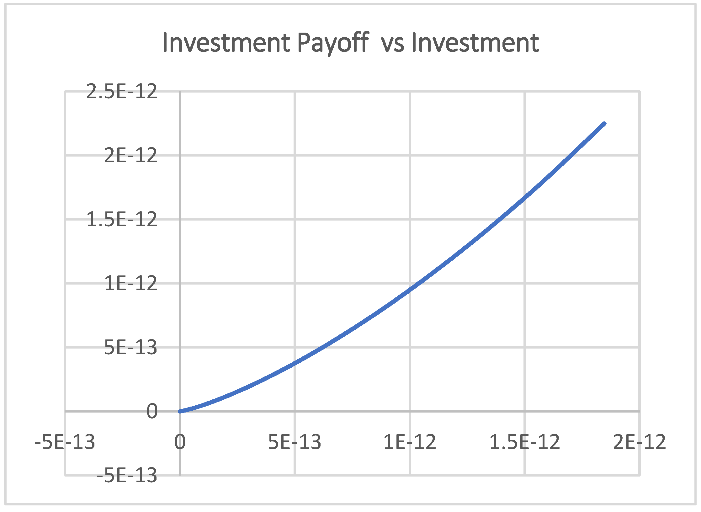
Figure 27.
Plot of Payoff (Inv & SP) vs IC.
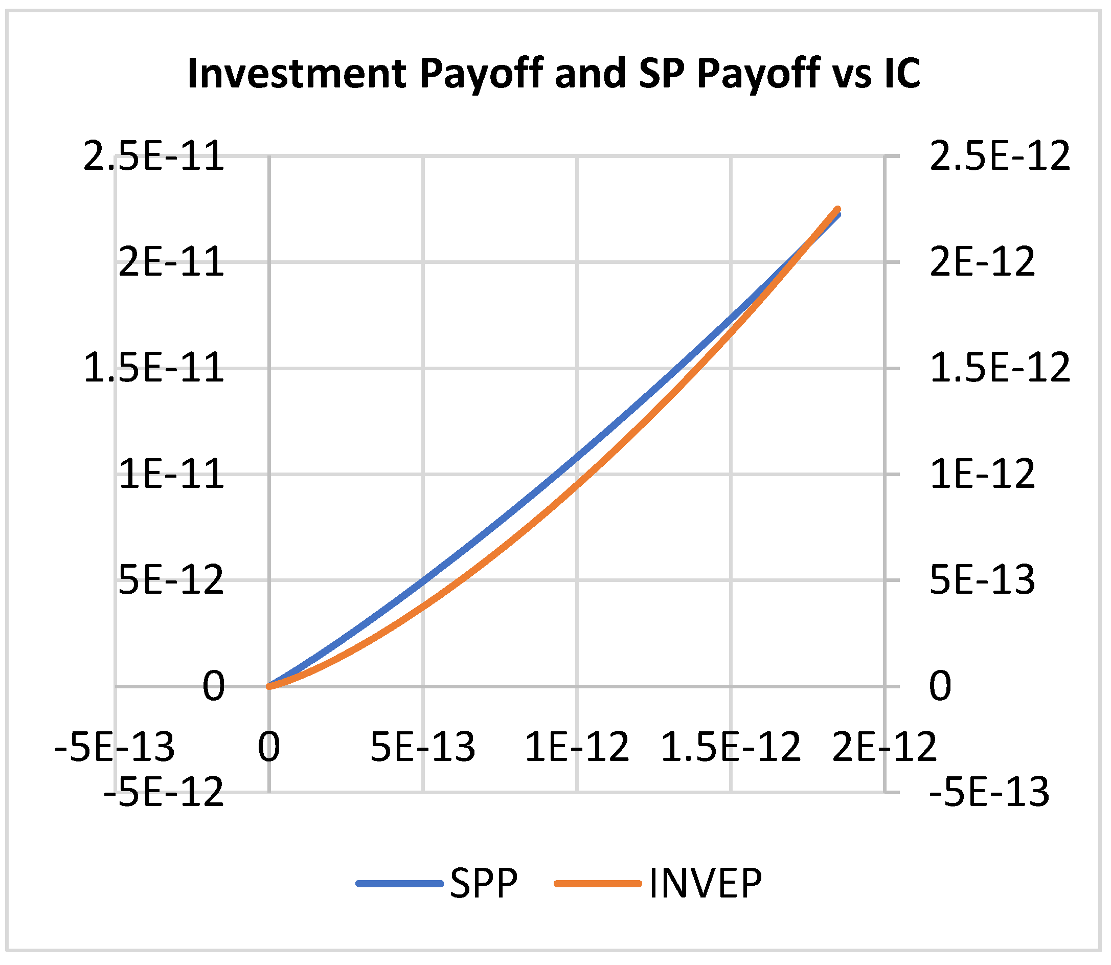
Figure 28.
Plot of Inv & Govt. vs SP Payoff.
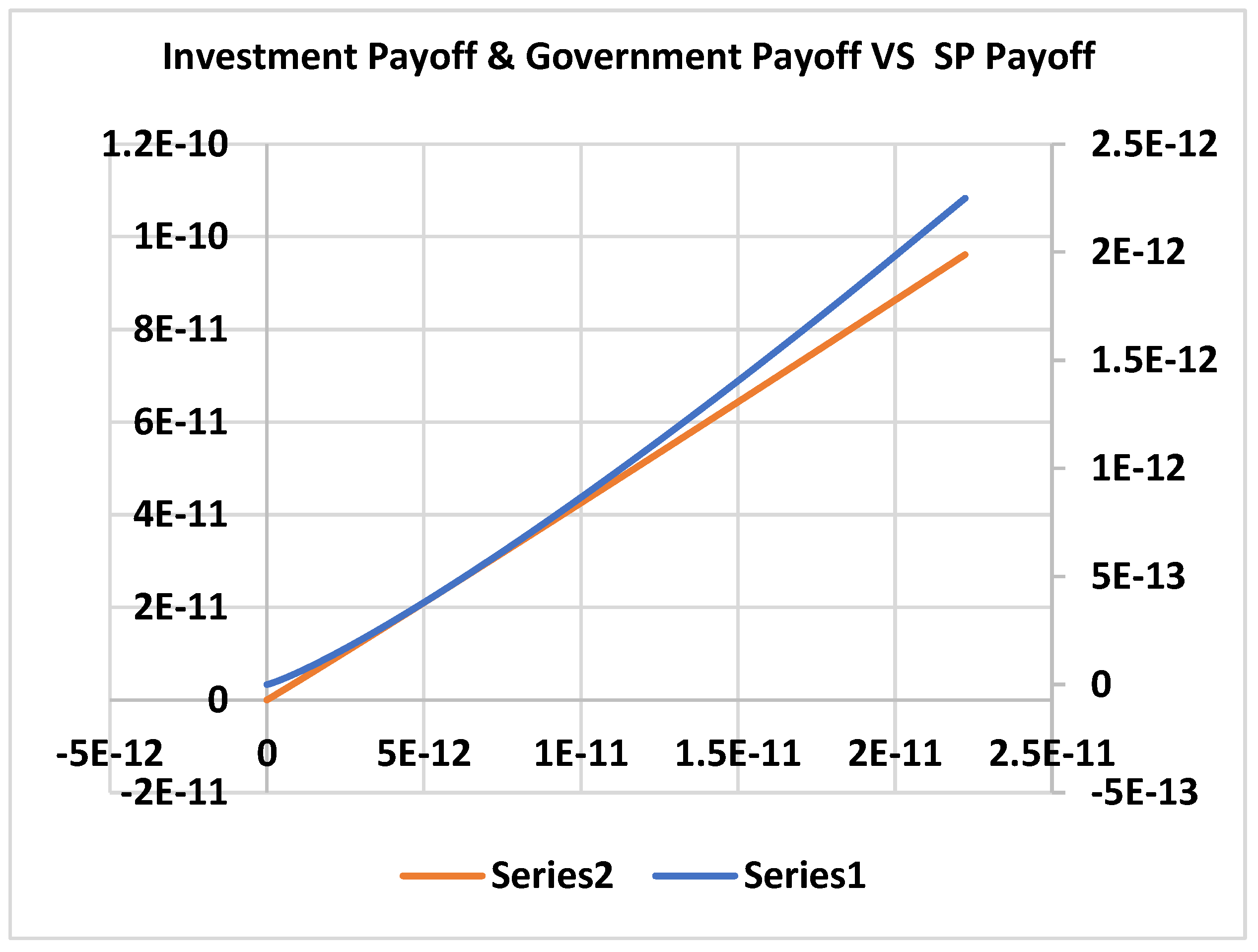
Figure 29.
Plot of SP Payoff Vs Effort.
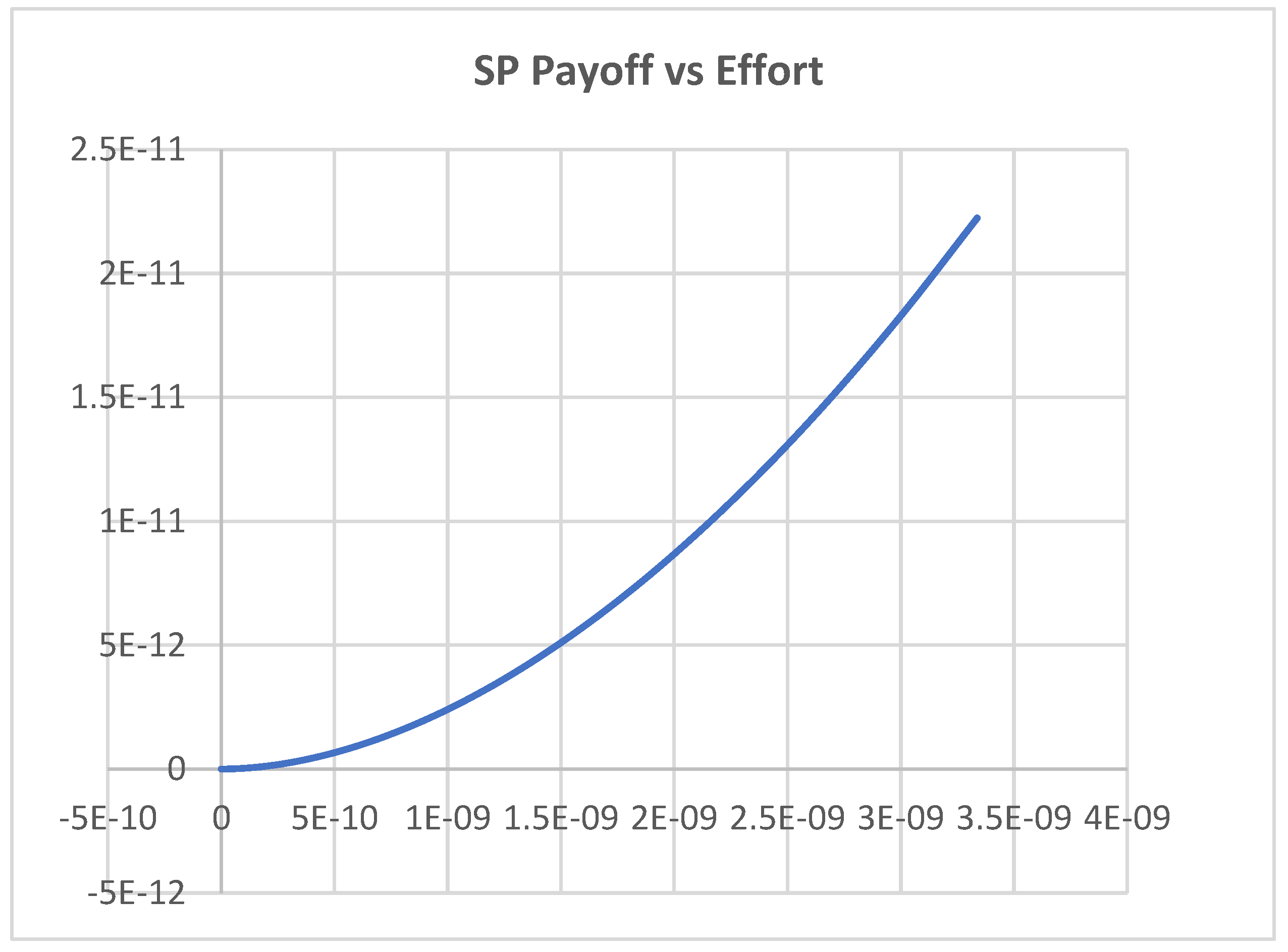
Figure 30.
Plot of Payoff (SP & Govt.) vs Effort.
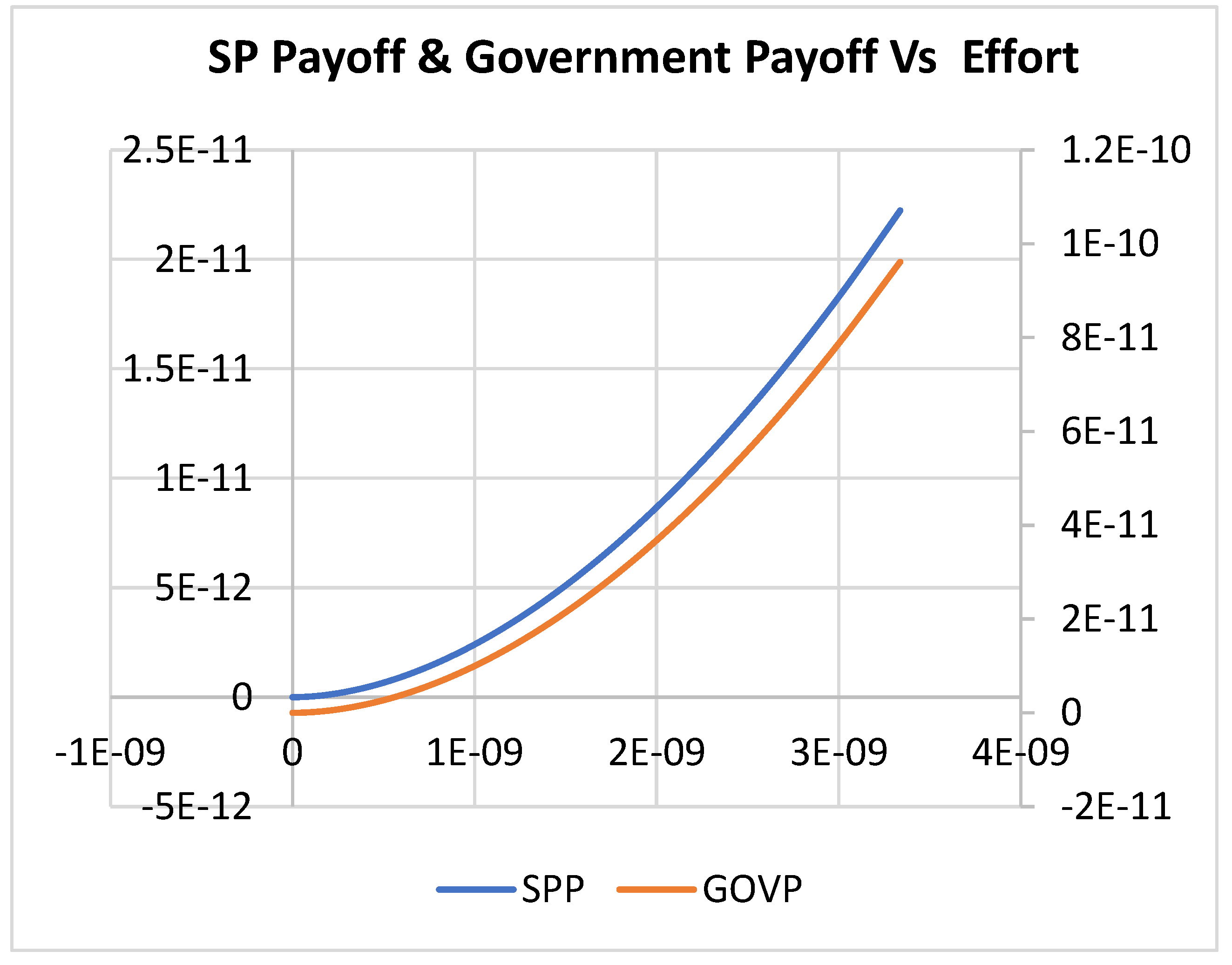
Figure 31.
Plot of Investment Payoff vs Effort.
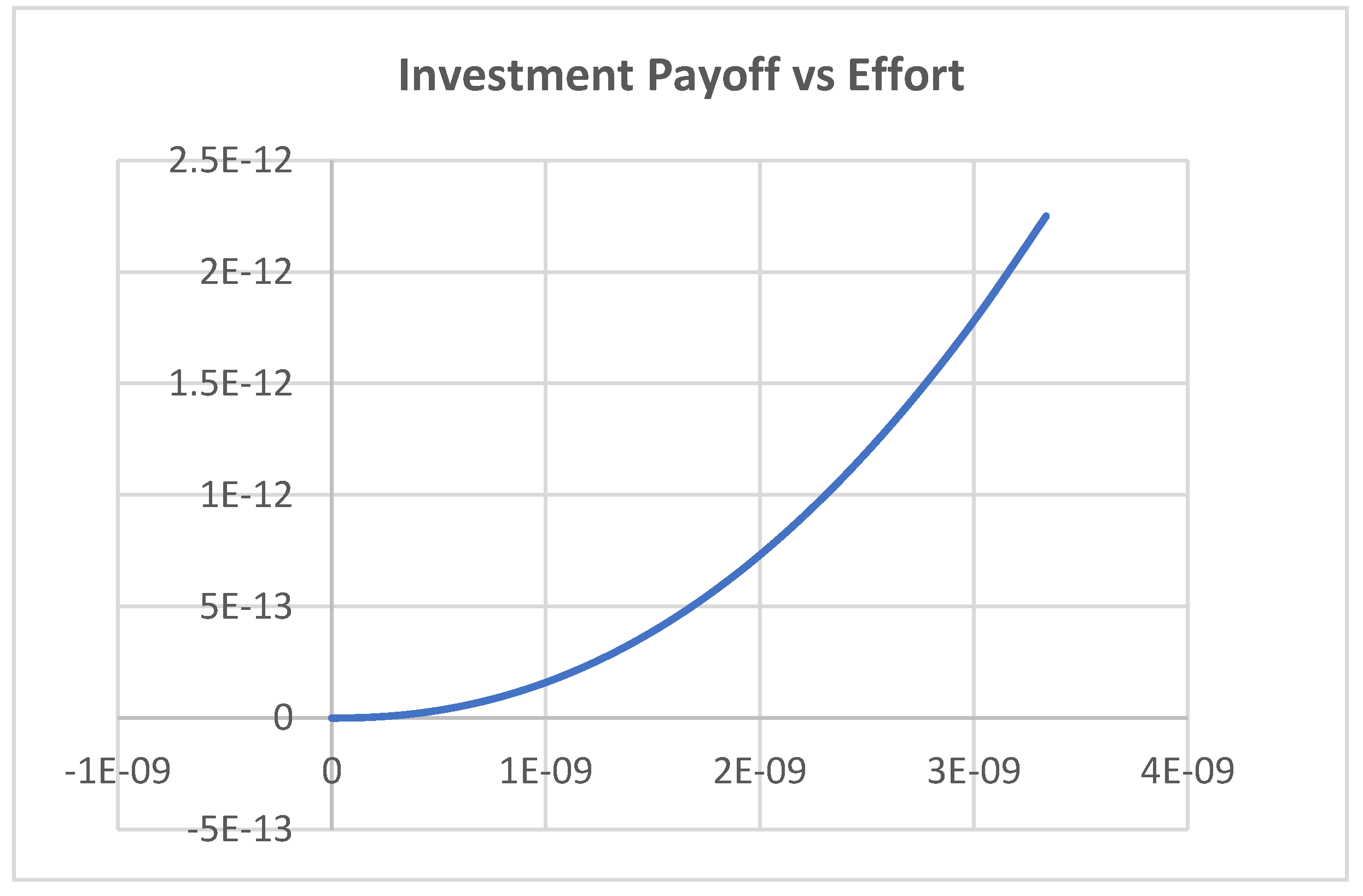

Table 1.
Summary of Results for Corporate Service Providers.
| Player | Service Provider (Corporate) | Government | Investor |
|---|---|---|---|
| Decision Variable | |||
| Corporate (Scenario 1) | |||
| Corporate (Scenario 2) | |||
| Corporate (Scenario 3) |
Disclaimer/Publisher’s Note: The statements, opinions and data contained in all publications are solely those of the individual author(s) and contributor(s) and not of MDPI and/or the editor(s). MDPI and/or the editor(s) disclaim responsibility for any injury to people or property resulting from any ideas, methods, instructions or products referred to in the content. |
© 2025 by the authors. Licensee MDPI, Basel, Switzerland. This article is an open access article distributed under the terms and conditions of the Creative Commons Attribution (CC BY) license (http://creativecommons.org/licenses/by/4.0/).
Copyright: This open access article is published under a Creative Commons CC BY 4.0 license, which permit the free download, distribution, and reuse, provided that the author and preprint are cited in any reuse.


