
Submitted:
11 June 2025
Posted:
12 June 2025
You are already at the latest version
Abstract
Efficient clustering of high-dimensional satellite image datasets remains a critical challenge, particularly due to the computational demands of spectral distance calculations, random centroid initialization, and sensitivity to outliers in conventional K-Means algorithms. This study presents a comprehensive comparative analysis of eight parallelized variants of the K-Means algorithm, designed to enhance clustering efficiency and reduce computational burden for large-scale satellite image analysis. The proposed parallelized implementations incorporate optimized centroid initialization for better starting point selection using a dynamic K-Means sharp method to detect the outlier to improve cluster robustness, and a Nearest-Neighbor Iteration Calculation Reduction method to minimize redundant computations. These enhancements were applied to a test set of 114 global land cover data cubes, each comprising high-dimensional satellite images of size 3712*3712*16, and executed on multi-core CPU architecture to leverage extensive parallel processing capabilities. Performance was evaluated across three criteria: convergence speed (iterations), computational efficiency (execution time), and clustering accuracy (RMSE). The Parallelized Enhanced K-Means (PEKM) method achieved the fastest convergence at 234 iterations and the lowest execution time of 4230 hours, while maintaining consistent RMSE values (0.0136) across all algorithm variants. These results demonstrate that targeted algorithmic optimizations, combined with effective parallelization strategies, can improve the practicality of K-Means clustering for high dimensional satellites image analysis. This work underscores the potential of improving K-Means clustering frameworks beyond hardware acceleration alone, offering scalable solutions good for large-scale unsupervised image classification tasks.
Keywords:
parallelized K-Means
; centroid initialization
; clustering quality
; computational efficiency
; hyperspectral images
; multispectral images
; iteration reduction
; outlier detection
; image clustering
; resource optimization
1. Introduction
1.1. Overview of Satellite Image
Satellite images are rich data sources crucial for providing geographical information[1]. For instance, the Landsat program has consistently provided high-quality multispectral images to help understand changes in land cover and the environment since 1972 [2]. Satellite remote sensing technologies collect data/images at variable revisit times, at diverse spatial, spectral, temporal and radiometric resolutions by sensors sensitive to specific spectral regions [3].
Satellite image clustering is a strong technique for deriving information and fulfills a crucial function across diverse applications, from land cover mapping and urban planning to environmental monitoring and disaster management [3]. The South Dakota State University (SDSU) Image Processing Lab (IPLAB) uses global image clustering as Extended Pseudo Invariant Calibration Site (EPICS) to calibrate satellites[4,5]. The purpose of image clustering is to group the pixels in the image to identify spectrally similar, homogenous sites with known spectral, spatial and temporal characteristics [6]. In contrast, information classes are categorical, such as crop type, forest type and residential type [7]. The advancement of improved clustering algorithms has gathered considerable attention. Previous implementations of the K-means clustering process within the IPLAB EPICS satellite calibration workflow consistently failed to reach the convergence threshold, preventing the algorithm from attaining a global minimum. Despite this, the resulting spectrally similar and temporally stable pixels were utilized in various satellite calibration effort, such as global EPICS classification for stability monitoring, validation of cross-calibration techniques, and inter-sensor comparison during on-orbit initialization [5,8,9]. However, the absence of convergence limited the robustness of site selection and contributed to increased uncertainty in radiometric calibration outcomes. The enhanced convergence properties of the proposed algorithms established a more stable foundation for future satellite calibration efforts, enabling reduced uncertainty and improved reproducibility in global-scale clustering outputs.
1.2. Related Work
1.2.1. Overview of Clustering Algorithm
Clustering algorithms are fundamental to unsupervised learning, enabling the partitioning of large datasets into meaningful groups without labeled training data [10,11]. In satellite image analysis, clustering enables the classification of pixels into land cover types on spectral characteristics. Common clustering algorithm includes hierarchical clustering [12], density-based method such as DBSCAN [13],spectral clustering [14,15], and partitioning algorithms like K-Means[16,17,18,19] . Each of these methods offers distinct advantages and trade-offs, particularly when applied to high-dimensional satellite imagery.
Hierarchical clustering provides a nested clustering structure or tree structure that allows flexible exploration of data groupings without predefining the number of cluster [20]. However, its computational complexity, typically O(n2logn)[21], renders it impractical for very large datasets like high-resolution satellite images exceeding millions of pixels per scene.
Density-based methods such as DBSCAN are effective in detecting clusters of arbitrary shapes and naturally handle noise and outliers[22]. Despite its advantages, DBSCAN faces significant challenges in high-dimensional data spaces, where the notion of density becomes less meaningful due to the curse of dimensionality. Moreover, its performance is highly sensitive to the choice of neighborhood radius (ε) and minimum points (MinPts), which complicates its application to large and diverse satellite datasets[23].
Spectral clustering[24] transforms the data into a graph-based representation and solves for eigenvectors of the Laplacian matrix to identify cluster. While powerful for handling non-convex clusters, spectral clustering suffers from prohibitive computational costs (O(n3)) associated with eigen decomposition, making it unsuitable for large-scale, high-dimensional image analysis.
In contrast, K-Means clustering [18,19,25,26] remains one of the most computationally efficient methods for large datasets , with the time complexity of O(n*k*i*d), where n is the number of data points, k is the number of clusters, i is the number of iterations, and d is the data dimensionality. K-Means is particularly well-suited to hyperspectral and multispectral satellite images due to its:
- Linear scalability with data volume;
- Support asynchronous parallel execution across independent data slices, enabling non-blocking processing of extremely large datasets (e.g. multiple 1 TB segments) by distributing computational task concurrently across multi-core or distributed systems;
- Flexibility to integrate algorithmic improvements such as advanced centroid initialization, iteration reduction, and outlier handling, as explored in this study.
Furthermore, modified K-Means facilitates high-performance parallel implementations using frameworks like MPI, OpenMP, and MapReduce, allowing effective distribution of computation across large CPU cluster[27,28,29] . This characteristic aligns closely with the architectural resources of our target HPC environment, which predominantly comprises CPU nodes, thus justifying the selection of K-Means as a fundamental algorithm for our optimization efforts.
1.2.2. Advancement in K-Means Clustering
Since its introduction by MacQueen in 1967[30] , the K-Means algorithm has undergone extensive refinement to address its inherent limitations, including sensitivity to initial centroid selection, vulnerability to outliers, and high computational demand on distance calculations [19].
One of the well-recognized limitations of Standard K-Means algorithm is its reliance on random selection for initial centroid positions, which can lead to poor convergence behavior and susceptibility to local minima [31]. To overcome this, several studies have proposed strategies to enhance centroid initialization. Khan et al. [32]proposed an improved initialization strategy that differentiates between instance attributes using a novel weighting formula, coupled with a specialized normalized process that avoids forcing values into restrictive range. However, the evaluation of this methodology on large-scale datasets and real-world scenarios remains limited. Chan et al. [33] introduced a hybrid method combining kernel K-Means ++ with random projection to reduce dimensionality before centroid selection. This approach successfully reduced computational complexity from O(n2D) to O(n2d), making it particularly suitable for high-dimensional clustering scenarios while preserving clustering quality. Nevertheless, while the method effectively reduces dimensionality, it does not address the issue of large sample size(n).
While these methods have demonstrated improvements over random selection aimed at improving clustering outcomes for complex and large-scale datasets. However, many of these techniques still encounter challenges related to computational load and scalability when applied to extremely high-dimensional data such as multispectral satellite imagery. To address this, our study proposes a uniform average pixel grouping strategy specifically designed for large-scale image clustering, which is detailed in Section 3.2.2.
The susceptibility of K-Means clustering to outliers is a challenge, often leading to skewed centroids and degraded clustering performance, especially in complex, high-dimensional datasets[34]. To overcome this issue, Olukanmi et al.[35] introduced K-Means sharp, a modified version of the classical K-Means algorithm that automatically detects outliers using global threshold derived from the distribution of point-to-centroid distances. However, as the authors acknowledged, the reliance on a single global threshold may not sufficiently capture local variations in outlier distribution across clusters. Building upon this foundation, CSK-Means and NSK-Means algorithms advanced the handling of outliers by incorporating density-based strategies and assigning separate clusters to outliers. These algorithms enhance robustness by considering the density within clusters and overlap spaces between them, making them capable of handling non-spherical cluster shapes and datasets with varying densities[36]. Despite these improvements, the authors noted that the algorithms require multiple iterative steps to determine the final cluster count in high-cluster scenarios, which can lead to elevate computational costs, especially in large-scale datasets. Recent advancements in anomaly detection have improved outlier detection in high-dimensional data, for instance, the ResAD framework proposed by Zhang et al. [37] focuses on class-generalizable anomaly detection by learning residual feature distributions, which can reduce feature variations and improve detection across diverse classes. However, ResAD’s effectiveness in clustering context remains to be thoroughly evaluated, and its integration into clustering frameworks like K-Means requires further investigation.
This study extends previous advancements by introducing a dynamic, cluster-specific thresholding approach within the K-Means Sharp framework. Thresholds are calculated individually for each cluster and dynamically update at every iteration to enhance clustering robustness. A detailed explanation of this refinement, including computational considerations and its application to large-scale satellite image analysis, is provided in Section 3.2.4.
Standard K-Means algorithm suffers from high computational cost due to the need to repeatedly calculate distances between every data point and all cluster centers at each iteration [38]. To address this, various methods have emerged focusing on reducing the number of distance calculations while maintaining clustering quality. Na et al.[39]proposed an improved K-Means algorithm that introduces a simple data structure to retain essential information across iterations, thereby eliminating redundant computations of distances to cluster centers. While this method effectively accelerates clustering, it primarily benefits datasets of moderate size and may struggle to scale efficiently for high-dimensional data or complex cluster boundaries. Wang et al. [40] further advanced this direction by identifying active points near cluster boundaries, enabling selective recalculation of cluster assignments. However, its effectiveness is heavily dependent on accurately identifying boundary points, making it less reliable in scenarios involving overlapping or irregular clusters. Moodi et al. [41] developed an improved K-Means variant for big data applications, leveraging the distances to two nearest centroids while excluding points beyond an equidistance threshold from further consideration. However, it faces challenges in handling large sample sizes, as its computational performance when the number of objects, dimensions and cluster increases.
To address these limitations in the context of satellite image clustering, this study proposes a Nearest-Neighbor Iteration Calculation Reduction Method that draws upon the strengths of prior work while adapting to the complexities of high-dimensional satellite datasets. Rather than relying solely on nearest-centroid tracking, the method incorporates a broader neighborhood context to better capture the nuances of spatial data distributions. While the technical specifics of this approach are detailed in section, it is well designed to balance computational efficiency with classification accuracy, making it well suited for clustering tasks involving diverse and overlapping land-cover types. The detail about this proposed method is explained in Section 3.2.3.
1.2.3. Parallelization Techniques in K-Means Cluster
To address the computational intensity of clustering high-dimensional data, parallelization strategies have become essential [42]. Early parallel K-Means implementation leveraged shared-memory architecture to distribute computations across multiple cores [43]. Subsequent development introduced block-processing techniques, effectively partitioning datasets for concurrent processing on multi-core CPUs[44]. Frameworks such as OpenMP and POSIX threads have demonstrated significant improvements in clustering performance by harnessing the full potential of modern processors[27].
GPU-accelerated implementation of K-Means have gained attention due to their massive parallel processing capabilities [45,46], particularly for real-time and high-throughput applications. However, in many high-performance computing (HPC) environments, including the one employed in this study, CPU nodes constitute the majority of available resources. The HPC system employed in this study comprises over 3000 CPU cores and only 14 GPU nodes. This resource distribution informed the strategic decision to optimize CPU-based parallelization, enabling full utilization of available computational capacity and achieving scalable performance for global land cover classification. This architecture strategically prioritizes CPU parallelization to efficiently manage I/O-bound operations by avoiding blocking calls. This asynchronous parallelization fully exploits available computational resources, enabling scalable performance for the classification of global land cover datasets. The implementation supports asynchronous parallel execution across independent data partitions, enhancing throughput and computational efficiency in large-scale image clustering tasks. Due to the high availability of CPU resources, the algorithm is optimized for CPU-based HPC environments; however, the design remains fully compatible with GPU processing, making it adaptable to diverse computing architectures.
1.2.4. Motivation and Contribution of This Study
While prior research has explored individual improvements in K-Means clustering algorithms and parallelization strategies, few studies have systematically evaluated multiple optimized variants under a unified framework, particularly at the scale required for global satellite image analysis. Existing methods have largely been tested on smaller or less complex datasets, leaving a gap in understanding their scalability and robustness when applied to extensive hyperspectral or multispectral image collections.
This study addresses this gap by conducting a comprehensive comparative analysis of eight parallelized K-Means variants, including enhancements in centroid initialization, outlier handling, and iteration reduction strategies. Performance evaluation was conducted using 114 high-dimensional data cubes representing diverse land cover types worldwide, with each method is assessed based on convergence speed, computational efficiency, and clustering quality. The insights gained from this analysis guide the selection of the most effective algorithms for future deployment across over the intended global data set of 9500 data cube in HPC environments. This work contributes to the advancement of scalable and efficient clustering techniques for large-scale remote sensing data classification purposes.
2. Materials
2.1. SDSU Dervied Data Product
Landsat 8 Operational Land Imager data were selected to generate the data cubes using Google Earth Engine (GEE), a cloud-based platform with high computational capabilities for processing large geospatial datasets[47]. The data filtering process addressed cloud cover and cloud shadows. For additional information, refer to Shrestha et al. [4] and Fajardo et al. [5].
2.2. Hardware and Software Specifications
This section describes the software and tools used to test all algorithms on identical datasets. The computational experiments were performed on a server equipped with an Intel Xeon Gold 6242R CPU @ 3.10GHz, featuring 2 sockets with 20 cores each, totaling 40 cores and 80 logical CPUs (2 threads per core). The software environment included the Linux operating system and MATLAB programming language.
Due to the large size of the test data, processing it in a single run was not feasible. Asynchronous parallel implementation of the algorithm utilized the “parfor” construct, analogous to job scheduling mechanisms, to process approximately 10 TB of data by calculating Euclidean distances and assigning pixels to clusters based on the shortest spectral distance. This approach was effective because each pixel value is independent of the others. Multicore, with 19 workers running concurrently, led to a significant reduction in computational time.
3. Methodology
Figure 1 shows the flowchart of the overall proposed framework. In the following section, the foundations of the approach are presented. For comparative analysis, the framework provides an overview of each algorithm. Landsat 8 images are input into eight different algorithms, each performing image segmentation through pixel classification. Clustering quality and computational efficiency are then evaluated using various performance metrics. Additional details about each method are provided in subsequent sections.
3.1. Satellite Imagery Dataset
To evaluate the performance of the parallelized versions of the modified K-Means algorithms, testing on all 9,522 data cubes in our archive is impractical. Consequently, a strategy was devised to select representative datasets based on different land cover types. Specifically, the Biosphere Atmosphere Transfer Scheme (BATS) Classification [48], was employed, categorizing land cover into 20 distinct classes. From this classification, 114 data cubes were selected, each representing a heterogeneous mixture of land cover types as seen in Figure 2. This approach ensures a comprehensive and efficient assessment of the algorithms' performance across diverse land cover scenarios. One data cube consists of a 1-8 temporal Mean and a 9-16 temporal standard deviation.

Table 1.
Parameters of Dataset and K-Means Clustering Algorithm.
| Parameter | Values |
|---|---|
| Data cube Number | 114 |
| Data cube Size | 3712*3712*16 (~1 GB) |
| # Cluster (k) | 160 |
| Convergent Criteria | 0.0005 |
3.2. Algorithm Development
The study involves a selection of parallelized modified versions of K-Means clustering algorithms using different variants of K-Means clustering processes. These modified versions mainly include three variants:
- Centroid Initialization Method
- Nearest-Neighbor Iteration Calculation Reduction Method
- Dynamic K-Means Sharp Method
3.2.1. Parallelize Standard K-Means Algorithms
The K-Means clustering algorithm is an iterative clustering technique that partitions a dataset into a predefined number of k distinct clusters, where each pixel is assigned to the cluster whose centroid has the closest mean value [19]. The process begins by randomly selecting k initial cluster centers, referred to as centroids, from each layer of the 114 data cubes, with each cube containing 3712*3712*16 pixels. These centroids serve as the initial reference points for the clusters.
where ‘m’ represents the number of clusters and ‘n’ represents the number of features.
The algorithm iteratively refines the clusters through the following steps. First, each pixel Pxyn is assigned to the nearest cluster based on the Euclidean distance. The Euclidean distance between a pixel Pxyn=(Pxy1, Pxy2,…, Pxy16) from the data cube of size 3712*3712*16 and a centroid μmn=([μ(1,1),μ(1,2),…,μ(1,16)],…,[μ(160,1),μ(160,2),…,μ(160,16)]), as seen in the Equation 2, where ‘m’ represents the number of centroids and ‘n’ represents the number of feature.
After all pixels have been assigned to clusters, the centroid for each layer of a cluster is calculated by using the following equation:
Equation 3 calculates the new mean, defined as the average of the pixel values assigned to the cluster. After calculating the new mean value, convergence is checked by comparing the old and new cluster mean. If the maximum difference between the old and new means exceeds a convergence threshold of 0.0005 then update the cluster mean with the new values and repeat the iterative process. This iterative approach gradually refines the clusters, making them more distinct and well-defined with each iteration. If the difference is below the threshold, the algorithm converges.
| Algorithm 1: Pseudocode for K-Means Algorithm | |
| Input: | I= {I1, I2, I3,….,Id} // set of d data cube ( 114 data cube with size 3712*3712*16 ) K // Number of desired clusters |
| Output: | A set of K distinct clusters |
| Step: | 1. Randomly select K initial cluster centers (centroids) from the 114 data cubes, where each centroid is represented by the matrix μmn as shown in Equation (1). 2. While max(|μmn,old - μmn,new |)<0.0005 do: 3. For (I=1: number_of_images)//for all images For (x=1: number_of_row) For (y=1: number_of_column)// for all pixel 4. Calculate the Euclidean distance between Pxyn and each centroid μmn using equation (2) 5. Assign Pxyn to the cluster with the nearest centroid (min(D(x,y,m))) 6. Update each centroid μmn: For each cluster m: 7. Calculate the new centroid using equation (3). 8. Check for convergence: 9. Calculate the maximum change in centroids: 10. DiffMean = max(|μmn,old - μmn_new|) 11. If DiffMean < 0.0005, then: Convergence achieved, exit loop 12. Else: Update centroids: μmn = μmn_new 13. Continue iteration End While |
When applying the K-Means clustering algorithm to 114 data cubes, each with dimensions 3712*3712*16, significant challenges are encountered related to speed-up, throughput, and scalability, particularly during the computation of the Euclidean distance between each pixel in the data cubes and the k centroids. Since the distance calculation for each pixel in different data cubes is independent, the process can be effectively parallelized asynchronously utilizing all resources making it computationally efficient.
To achieve this parallelization in MATLAB, the ‘parfor’ loop is utilized which is analogous to job scheduling mechanism in slurm, allowing asynchronous parallelization of task to run concurrently on multiple worker sessions. The process begins by opening a MATLAB pool, which allocates a set of MATLAB worker sessions. These workers are then assigned to handle clustering tasks, where the worker processes a subset of the data cubes – specifically, N/n data cubes, where N is the total number of data cubes and n is the number of workers.
Parallel execution allows for efficient distance computation by distributing workloads among available compute node, as shown in Figure 3. Each node independently processes assigned data chunks, gathers results, and updates centroids upon completion. This process continues until the convergence criteria are met, ensuring iterative refinement of clusters. Figure 4 illustrates the operation flowchart of this parallelization, showing how data chunks are distributed to workers and how results are combined.
Algorithm 2 provides the pseudocode for the parallel implementation of Standard K-Means clustering algorithm, which is implemented using the ‘parfor’ function on the server. Details about the hardware and software used for this implementation are described in Section 2.2.
| Algorithm 2: Pseudocode for Parallelization Standard K-Means algorithm | |
| Input: | I={I1, I2, I3,….,In} // set of d data cube ( 114 data cube with size 3712*3712*16 ) K // Number of desired clusters |
| Output: | A set of K distinct clusters |
| Step: | Randomly select K initial cluster centers (centroids) from the 114 data cubes, where each centroid is represented by the matrix μmn as shown in Equation (1). While max(|μmn,old - μmn,new |) < 0.0005 do: Parfor each Data chunk I={I1, I2,I3,..,Id} For (x=1: number_of_rows) For (y=1: number_of_columns) Calculate the Euclidean distance between Pxyn and each centroid μmn using Equation 2. Assign Pxyn to the cluster with the nearest centroid (min(D(x,y,m))) Calculate the partial sums for each cluster for updating centroids End Parfor Combine partial sums from all chunks to calculate the new mean (centroid) for each cluster. Update each centroid μmn: For each cluster m: Calculate the new centroid using equation (3). Check for convergence: Calculate the maximum change in centroids: DiffMean = max(|μmn,old - μmn_new|) If DiffMean < 0.0005, then: Convergence achieved, exit while loop Else: Update centroids: μmn = μmn_new Continue iteration End While |
In line 3 of Algorithm 2, the “parfor” function leverages the multicore capabilities of the CPU to compute distances and assign pixels to the nearest cluster. This parallelization is consistently applied across all modified versions of the K-Means algorithms.
3.2.2. Parallelize Centroid Initialization Method
This improved algorithm introduces a new method to calculate a uniform average across the dataset. Pixel values are extracted through a 100×100 grid to create a matrix. Afterward, the matrix was subsequently sorted based on the fifth column, corresponding to the Near-Infrared (NIR) band, due to its relative insensitivity to atmospheric effects and its capacity to distinguish surface variability. Rows containing NaN values were removed to ensure data integrity prior to further processing. Initial centroids are determined by dividing the matrix into 160 groups and calculating the average for each group. Refer to Algorithm 3 for the pseudocode related to class initialization.
| Algorithm 3: Pseudocode for class initialization of parallel centroid initialization method | |
| Input: |
I={I1, I2, I3,….,In} // set of n data cube ( 114 data cube with size 3712*3712*16 ) K //Number of desired clusters |
| Output: | A set of K distinct clusters. |
| Step: | sampledpixelvalues ← 10*10 matrix of zeros (size: 100 x 16) counter← 1 For (i = 1 to 114): imagein ← read image from Imagefile Select only the first 16 layers of the image: imagein ← imagein(:,:,1:16) image ← imagein(:,:,5) // Select band 5 for operations Set grid size: gridsize ← 371 Calculate number of grid points: numpointX ← floor(size of image in dimension 1 / gridsize) numpointY ← floor(size of image in dimension 2 / gridsize) For each grid point, extract pixel values: For j = 1 to numpointX: For z = 1 to numpointY: Calculate x and y based on grid index: x ← (j - 1) * gridsize + 1 y ← (z - 1) * gridsize + 1 Assign sampled pixel values to sampledpix- elvalues [counter,:] ← imagein(x, y, :) Counter Increment Save the sampled pixel values: Sort the sample pixel values by the 5Th Column: columntosortby ← sampledpixelvalues(:, 5) sortedvalues, sortedindices ← sort(columntosortby) sortedMatrix ← sampledpixelvalues(sorted by sortedindices) Remove rows containing NaN values: rowswithnans ← any(isnan(sortedMatrix)) sortedMatrix ← sortedMatrix without rowswithnans Calculate the Initial centroid: row, column ← size(sortedMatrix) rows_per_group ← floor (row / 160) remainder ← mod (row, 160) InitialCluster ← 160 x column matrix of zeros Group rows and calculate mean for each group: start_index ← 1 For (i = 1 to 160): If i ≤ remainder set end_index ← start_index + rows_per_group Else Set end_index ← start_index + rows_per_group - 1 Currentgroup ← sortedMatrix[startindex:endindex, :] Calculate mean for the current group and store in InitialCluster[i, :] ← mean(currentgroup) Update startindex ← endindex + 1 Save the calculated initial centroids. |
Algorithm 3 introduces a more effective method for determining the initial centroids of clusters, unlike the Standard K-Means Algorithm, which chooses centroids randomly. This improvement accelerates the convergence of the K-Means clustering algorithm.
Moreover, the revised K-Means algorithm incorporates data vectorization into a 2D matrix, making Euclidean distance calculations as seen in Equation 4 more efficient. While Algorithm 2 relies on two 'for' loops to extract pixels from the image, the optimized Algorithm 4 streamlines this task using a single loop.
| Algorithm 4: Pseudocode for main classification |
|
Parfor each Data chunk I={I1, I2,I3,..,Id} Reshape the image data into 2D array For (x=1:number_of_row) Calculate the Euclidean distance between Px,n and each centroid μmn using Equation 4 Assign Px,n to the cluster with the nearest centroid (min(D(x,m))) Calculate the partial sums for each cluster for updating centroids End Parfor |
As shown in Algorithm 4, the reshaping of a 16-dimensional tensor is vectorized into a 2-dimensional tensor. This modification eliminates the need for a single 'for' loop in Euclidean distance calculation as seen in Equation 4, while other steps remain similar to those in Algorithm 2.
3.2.3. Parallelized Nearest-Neighbor Iteration Calculation Reduction Method
To address the computational inefficiency in the Standard K-Means algorithm, this study introduces a Nearest-Neighbor Iteration Reduction Method, enhancing the accuracy of classification while minimizing redundant distance calculations. Unlike the Iteration Reduction Method proposed by Na et al. [39], which stores only the closest cluster for each pixel and recalculates distances during every iteration, the proposed method maintains the distances to the fifteen nearest cluster for each pixel. Assigning cluster based only on the nearest centroid can result in misclassification, especially near cluster boundaries or in data with irregular shapes and varying densities, while considering multiple nearest centroids improves accuracy by better reflecting the data’s distribution.
As shown in Algorithm 2, the distance calculation from each pixel to all k cluster centers during each iteration consumes a significant amount of execution time, particularly for large datasets like multispectral images. The core concept of this approach involves utilizing two fundamental data structures to store the closest cluster label and the corresponding distance of each pixel to its nearest cluster at every iteration, allowing this information to be used in the subsequent iteration. For each pixel, its distance to the nearest cluster is stored. In the subsequent iteration, the algorithm first computes distances to the previous 15 nearest clusters. A condition states that if pixels are assigned to a cluster beyond the 12 nearest or if the previous shortest distance exceeds the current shortest distance among 15 neighbors, distance to all clusters are recalculated, and nearest clusters are updated accordingly. The reason for selecting the 15-12 combination is based on computational speed. An experiment with different combinations (10,5), (15,10), and (15,12)—was conducted using a small dataset of 20 data cubes to determine which combination converges faster. Results show that saving 15 neighbors and assigning pixels with 12 nearest neighbors helps achieve faster convergence.
| Algorithm 5: Pseudocode for Parallelize Nearest-Neighbor Iteration Calculation Reduction Method | |
| Input: | I={I1, I2, I3,….,Id} // set of d data cube ( 114 data cube with size 3712*3712*16 ) K // Number of desired clusters |
| Output: | A set of k clusters. |
| Step: | Randomly select K initial cluster centers (centroids) from the 114 data cubes, where each centroid is represented by the matrix μmn as shown in Equation (1). While max(|μmn,old - μmn,new |) < 0.0005 do: Parfor each Data chunk I={I1, I2,I3,..,Id} Reshape the image data into 2D array For (x=1 : number_of_row) Calculate the Euclidean distance between Pxn and each centroid μmn using Equation 2. Reshape back to original dimension Assign Pxyn to the cluster with the nearest centroid (min(D(x,y,m))). Store the labels of 15 nearest cluster centers for pixel Pxyn in the arrays Cluster_Label[]. Separately store the distance of Pxyn to the nearest cluster in Closest_Dist[]. Set Cluster_Label[]=k(the indices of the 15 nearest clusters). Set Closest_Dist[x,y]=D(Pxyn, μmn ); (the minimum distance to the closest cluster). Calculate the partial sums for each cluster for updating centroids End Parfor Update each centroid μmn: For each cluster m: Calculate the new centroid using equation (3). Update centroids: μmn = μmn_new Repeat Parfor each Data chunk I={I1, I2,I3,..,Id} Reshape the image data into 2D array Calculate the distance between the pixel and the centroids of the 15 nearest clusters stored in Cluster_Label[]. Identify the rank of the currently assigned cluster within the 15 nearest clusters: If the currently assigned cluster is within the top 12 nearest clusters, no recomputation is required. If the currently assigned cluster is ranked between the 13th and 15th nearest clusters or the pixel has not been assigned, then go for the recomputation of pixel between all the cluster. End parfor; For each cluster m, (1<=m<=K), recalculate the centroid. Until the convergent criteria is met (previous centroid – new centroid) < 0.0005 |
The first step of the algorithm involves calculating the Euclidean distance from each pixel to initial centroids of all clusters using Equation 4. Each Pixel is allocated to the nearest centroid, forming an initial pixels group. For every pixel, the cluster assignment (Cluster_Label[]) and its proximity to the nearest cluster centroid (Closest_Dist[]) are recorded. Additionally, the labels of the 15 nearest cluster centers are stored in the arrays Cluster_Label[], while the distance to the nearest cluster is separately stored in Closest_Dist[]. As pixels are assigned to different clusters, the values of the cluster centroids may change. Centroids are iteratively recomputed for each cluster by averaging the pixel values within the respective cluster. Up to this point, the procedure is similar to Algorithm 2.
The next step is an iterative process that employs a heuristic method to improve efficiency. During the subsequent iteration, the algorithm focuses on optimizing cluster assignments by leveraging the distance between each pixel and the centroids of its fifteen nearest clusters. At the start of each iteration, the distances to these fifteen nearest centroids, stored from the previous iteration, are recalculated. If the pixel remains assigned to a cluster within its top twelve nearest clusters, no further computation is required for that pixel. This approach reduces unnecessary distance calculation to all the clusters, saving computation time.
However, if the pixel is assigned to a cluster ranked between the thirteenth and fifteenth nearest or the new distance to its nearest cluster exceeds the previously stored distance, the algorithm recalculates distances between the pixel and all cluster centroids. This ensures accurate reassignment to the closest cluster. Additionally, pixels marked for recomputation undergo a similar process to identify the new nearest cluster, and the Cluster_Label and Closest_Dist arrays are updated accordingly. This iterative refinement continues until the movement between centroids stabilizes, defined by a threshold of 0.0005, ensuring convergence.
3.2.4. Parallelize Dynamic K-Means Sharp Method
Olukanmi et al. [35]proposed the K-Means Sharp Method, which modifies the Standard K-Means centroid update step to exclude outliers during centroid calculation. The adaptation introduction global threshold values for all cluster. However, the method is extended to the Dynamic K-Means Sharp Method by incorporating spatial standard-deviation measurements of cluster to identify and manage both inlier and outlier pixels within individual clusters.
Outlier Detection
K-Means operates on the assumption that the data follows a Gaussian distribution, meaning that most inliers will fall within ±3 standard deviations of the centroid. This range corresponds to the area under the normal distribution curve within ±3σ of the mean, where most data points are expected to be located. Any point outside this range is considered outlier.
For each band of a cluster, the spatial standard deviation was calculated. Consequently, the pixel-to-centroid distance threshold, T , which differentiates inliers from outliers, is defined as:
where is the spatial standard deviation of cluster per feature, 1<=m<=K (centroid) and 1<=n<=feature.
Note that T is a cluster and band specific threshold value in contrast to single global value that applies across all clusters which is proposed by Olukanmi et al. [35].
New Centroid update
With an appropriate value of T calculated as per Equation 5, this method identifies inlier and outlier pixels for each spectral band based on their distance from the cluster mean (centroid) and the cluster's standard deviation. Inliers are pixels that lie within 3 standard deviations of the mean for each feature, while outliers are those outside this range. For each cluster feature, the new centroid is recalculated by averaging only the inlier pixels, effectively minimizing the impact of outlier pixels on the centroid’s position.
where is the set of the pixels in that have pixel-to-centroid
The mean for each cluster is calculated using two approaches outlined in Equations 2 and 6. Both approaches define a new centroid as the mean of the pixels associated with each respective band and cluster. However, Equation 6 differs by excluding pixels that lie beyond a distance T from the cluster centroid. This exclusion refines the centroid calculation by reducing the impact of outlier pixels.
Pixel classification follows the same method as in Algorithm 2. The primary change in this approach is in the centroid update step. Instead of recalculating centroids by averaging all pixels within each cluster, this modified algorithm identifies and excludes potential outliers from the computation.
| Algorithm 6: Pseudocode for Parallelize Dynamic K-Means Sharp Method | |
| Input: | I={I1, I2, I3,….,Id} // set of d data cube ( 114 data cube with size 3712*3712*16 ) K // Number of desired clusters |
| Output: | A set of k clusters. |
| Step: | Randomly select K initial cluster centers (centroids) from the 114 data cubes, where each centroid is represented by the matrix μmn as shown in Equation (1). While max (|μmn,old - μmn,new |)<0.0005 do: Parfor each Data chunk I={I1, I2,I3,..,Id} Reshape the image data into 2D array For (x=1 : number_of_row) Calculate the Euclidean distance between Pxn and each centroid μmn using Equation (3). Reshape back to original dimension Assign pixel Pxyn to the cluster with the nearest centroid (min(D(x,y,m))). Calculate the partial sums for each cluster for updating centroids END Parfor Update each centroid μmn: For each cluster m: Calculate the new centroid using equation (3). Update centroids: μmn = μmn_new Calculate Spatial Standard deviation For each data chunk, calculate the sum of squared difference for each band of clusters squared_diff=(Meantile-NewCluster)2 Accumulate the sum across all data cubes. Compute the standard deviation for each cluster and band: std_values=sqrt(sum_squared_diff/count) Repeat Parfor loop to update pixel assignments: Compute inliers and outliers based on the spatial standard deviation: For each cluster and band: get pixels in the current cluster and compute the absolute difference pixels and the cluster mean for each band. inliers are those within 3*std_value. inliers=abs(cluster_pixel(:,feature)- mean_value)<=3*std_value Update inlier count and calculate partial sums for the next centroid update: Inlier_count(cluster,band)+=sum(inliers) MeanCluster(cluster,band)+=sum(cluster_pixel(inliers,band)) Outlier count: Outlier_count(cluster,band)=total_pixel_in_cluster-inlier_count(cluster,band) End Parfor Update the cluster centroids based on inliers using equation 5. Until the convergent criteria is met (previous centroid – new centroid) < 0.0005 |
In the dynamic K-Means sharp algorithm, the process starts by randomly initializing the cluster centroids from the data cubes. Each iteration assigns pixels from the data cubes to the nearest centroid based on Euclidean distance, computed in parallel using a "parfor" loop to handle the large dataset. Each pixel is assigned to the centroid with the minimum distance, and partial sums are calculated in parallel to gather the data needed for updating the centroid. After the parallel step, the partial sums from all data chunks are combined to compute new centroids for the clusters, and the algorithm checks for convergence. If the maximum change in the centroids is smaller than a threshold (0.0005), the algorithm converges. Otherwise, the centroids are updated, and the process repeats.
In later iterations, the algorithm incorporates spatial standard deviations for each cluster. After parallel processing of pixel assignments, the spatial standard deviation is calculated based on the squared difference between the current centroids and the pixel values for each band. Pixels within three standard deviations of the mean for each cluster and band are considered inliers, while those outsides are considered outliers. The inliers are used to update the centroids using Equation (6). The algorithm continues this iterative process, recalculating the centroids and spatial standard deviations in each iteration until convergence.
3.2.5. Integrated Variant Comparisons
In this section, the performance of various K-Means clustering algorithm variants implemented in a parallelized manner is examined. Specifically, the focus is on how each parallelized variant performs when combined with other algorithm modifications. This implementation also divides the dataset into chunks and distributes them to processing units, where clustering occurs in parallel.
Table 2.
Specific Combinations of three Variants.
| Combination Name | Centroid Initialization Algorithm | Nearest-Neighbor Iteration Calculation Reduction Algorithm | Dynamic K-Means Sharp Algorithm |
|---|---|---|---|
| Parallel Combination 1 | 1 | 0 | 1 |
| Parallel Combination 2 | 0 | 1 | 1 |
| Parallel Combination 3 | 1 | 1 | 0 |
| Parallel Enhanced K-Means (PEKM) | 1 | 1 | 1 |
Parallel combination 1 (Combination of Centroid Initialization and Dynamic K-Means Sharp Method)
This combination integrates the Centroid Initialization Algorithm with the Dynamic K-Means Sharp algorithm to enhance accuracy. Detailed steps for this improved method are provided in Algorithm 7.
| Algorithm 7: Centroid Initialization and Dynamic K-Means Sharp Method | |
| Input: |
I= {I1, I2, I3,….,Id} // set of d data cube ( 114 data cube with size 3712*3712*16 ) K // Number of desired clusters |
| Output: | A set of k clusters |
| Step: | Phase 1: Identify the initial cluster centroids by using Algorithm 3 Phase 2: Update centroid by using Algorithm 6 |
In the first phase, the initial centroids are systematically set to form clusters with enhanced accuracy, as outlined in Section 3.2.2. The second phase applies to a variant of the clustering method from Section 3.2.4. This phase begins by creating initial clusters based on the uniform average of grouped pixels, as explained in Algorithm 3. These clusters are then refined using the K-Means Sharp method, which updates centroids by excluding outliers. Detailed steps for these two enhanced methods are provided in Algorithms 3 and 6.
Parallel combination 2 (Combination of Nearest-Neighbor Iteration Calculation Reduction and Dynamic K-Means Sharp Method)
This approach combines Iteration Calculation Reduction with the Dynamic K-Means Sharp algorithm to enhance computational efficiency and accelerate convergence while maintaining clustering accuracy. The detailed steps of this method are provided in Algorithm 8.
| Algorithm 8: Dynamic K-Means Sharp and Nearest-Neighbor Iteration Calculation Reduction Method | |
| Input: |
I={I1, I2, I3,….,Id} // set of d data cube ( 114 data cube with size 3712*3712*16 ) K // Number of desired clusters |
| Output: | A set of k clusters |
| Step: | Phase 1: Assign each data point to the appropriate cluster by Algorithm 5. Phase 2: Update centroid by using Algorithm 6 |
In the first phase, a variant of the clustering method discussed in Section 3.2.3. is employed to improve efficiency. The second phase utilizes a variant of the clustering method outlined in Section 3.2.4. The two phases of this enhanced method are detailed in Algorithm 5 and Algorithm 6.
Parallel combination 3 (Combination of Centroid Initialization and Nearest-Neighbor Iteration Calculation Reduction Method)
By merging the Centroid Initialization Algorithm and Iteration Calculation Reduction, this combination is designed to improve convergence rates while maintaining accurate cluster assignments.
| Algorithm 9: Centroid Initialization and Nearest-Neighbor Iteration Calculation Reduction Method | |
| Input: |
I={I1, I2, I3,….,Id} // set of d data cube ( 114 data cube with size 3712*3712*16 ) K // Number of desired clusters |
| Output: | A set of k clusters |
| Step: | Phase 1: Identify the initial cluster centroids by using Algorithm 3 Phase 2: Assign each data point to the appropriate cluster by Algorithm 5 |
The first phase employs a variant of the clustering method discussed in Section 3.2.2, aimed at enhancing efficiency. In the second phase, another variant of the clustering method, outlined in Section 3.2.3, is used. Detailed descriptions of both phases in this enhanced method appear in Algorithms 3 and 5.
Parallel Enhanced K-Means Method (PEKM)
This comprehensive combination integrates all three variants: the Centroid Initialization Method, Nearest-Neighbor Iteration Calculation Reduction Method, and Dynamic K-Means Sharp Method. By leveraging the strengths of each approach, the method ensures efficient and improved clustering quality, maximizing both performance and precision.
| Algorithm 10: Centroid Initialization Method, Dynamic K-Means Sharp, and Nearest-Neighbor Iteration Calculation Reduction Method | |
| Input: |
I={I1, I2, I3,….,Id} // set of d data cube ( 114 data cube with size 3712*3712*16 ) K // Number of desired clusters |
| Output: | A set of k clusters |
| Step: | Phase 1: Determine the initial centroids of the clusters by using Algorithm 3 Phase 2: Assign each data point to the appropriate cluster by Algorithm 5. Phase 3: Update centroid by using Algorithm 6 |
In the first phase, the initial centroids are systematically determined, as described in Section 3.2.2. The second phase uses a variant of the clustering method discussed in Section 3.2.3, while the third phase applies another variant outlined in Section 3.2.4. The three phases of this enhanced method are detailed in Algorithms 3, 5, and 6.
3.3. Convergent Criteria
In K-Means clustering, pixels get assigned to clusters, and centroid updates continue until meeting specific stopping criteria. Possible criteria include:
- Reaching a predetermined maximum number of iterations.
- Having fewer pixel reassignments per iteration than a set threshold.
- Centroid shifts fall below a specified distance threshold during an update cycle.
For this project, convergence was determined using centroid migration threshold of 0.0005 (0.05 reflectance units), a value adopted from the work of Shrestha et al.[4], where it was shown to effectively optimize cluster compactness.
3.4. Performance Metrics
As datasets in remote sensing continue to grow, reducing computational costs has become crucial due to the increasing demand for computational power. The methodology section outlines the various methods implemented to address this challenge. The model's effectiveness was evaluated using the following performance metrics.
3.4.1. Convergence Speed
The iteration count required for the algorithm to meet the threshold condition represents a primary performance metric. Evaluating each parallel K-Means variant reveals which version converges with the fewest iterations.
3.4.2. Clustering Quality
The quality of clustering in the K-Means algorithm can be evaluated using several methods, including the Silhouette Coefficient[49], Calinski-Harabasz Index [50], and Mean Square Error (MSE)[19]. However, due to the computational expense and infeasibility of these methods for high-dimensional data, the Root Mean Square Error (RMSE)[51] was chosen for evaluation. The RMSE is calculated through the following steps:
1.
73.
74.
75. Compute the Root Mean Square Error:
76. Compute the Average Root Mean Square Error:
where:
- Vij : The jth valid pixel in the ith cluster.
- Cik : The centroid value for the kth band of the ith cluster.
- Ni : The number of valid pixels in the ith cluster.
- C : Total number of clusters.
- B : Total number of bands.
3.4.3. Computational Efficiency
Evaluating computational efficiency involves measuring the execution time required for each parallelized K-Means algorithm variant to reach the specified convergence threshold. A comparison of execution times highlights the most efficient algorithms.
3.5. Comparative Analysis
This study provides a comparison of parallelized, modified versions of K-Means clustering algorithms based on selected performance metrics. Experiments were conducted on identical datasets to ensure consistency and enable a direct comparison of algorithm performance.
4. Evaluation and Experimental Results
This study primarily aims to enhance the standard K-Means clustering algorithm by accelerating its convergence, improving computational efficiency, and maintaining similar clustering compactness. This section discusses the findings derived from optimized variants of the K-Means clustering algorithm, as described in Section 3.2. The evaluation includes an analysis of convergence speed, clustering quality, and computational efficiency for each optimization technique described in Section 3.4, with a focus on their effectiveness in handling high-dimensional satellite imagery.
4.1. Convergent Speed Comparison
Convergence speed is a critical metric for assessing the efficiency of parallelized K-Means algorithm, measured by the number of iterations needed to achieve convergence. The criterion for cluster convergence is determined by the displacement of centroids between the previous and the most recently computed centroid positions.
For clarity in figures and tables, abbreviated method names are used. The corresponding full method descriptions are provided in Table 3.
Table 3.
Method Abbreviation for Parallelized K-Means Algorithm.
| Method Abbreviation | Full Method Description |
|---|---|
| PSKM | Parallelized Standard K-Means Algorithm |
| PSKM+CI | Parallelized Centroid Initialization Method |
| PSKM+KS | Parallelized Dynamic K-Means Sharp Method |
| PSKM + NN | Parallelized Nearest-Neighbor Iteration Calculation Reduction Method |
| PSKM + CI + KS | Parallelized Centroid Initialization and Dynamic K-Means Sharp Method |
| PSKM + CI +NN | Parallelized Centroid Initialization and Nearest-Neighbor Iteration Calculation Reduction Method |
| PSKM + KS + NN | Parallelized Dynamic K-Means Sharp and Nearest-Neighbor Iteration Calculation Reduction Method |
| PEKM | Parallelized Enhance K-Means Method |
Figure 5 illustrates the convergent speed of parallelized modified K-Means algorithms over iterations. On the graph, the x-axis indicates the number of iterations, whereas the y-axis depicts the displacement of centroids between consecutive iterations. Each line corresponds to a specific parallelized modified K-Means algorithm. The results also demonstrate that centroids stabilize with respect to iteration. Please refer to Table 3 for the description of Abbreviated method
The Parallelized Standard K-Means algorithm (Blue color with diamond) failed to converge within the tested iterations. However, incorporating improvements such as selecting initial centroid deterministically, applying Dynamic K-Means Sharp for removing the outlier from getting into the calculation of centroid, and using the previous information of assigned cluster to pixel and assigned distance to reduce computational complexity arises because of classification of pixel, enabled convergence for the Parallelized Standard K-Means algorithm under specific conditions. The following observations were made regarding the convergence of the modified algorithms where the convergence threshold is set to 0.0005.
Table 4.
Number of iterations required for convergence across Parallelized K-Means methods.
| Method | Iterations till convergence |
|---|---|
| PSKM+CI | 348 iterations |
| PSKM+KS | 282 iterations |
| PSKM + NN | 326 iterations |
| PSKM + CI + KS | 257 iterations |
| PSKM + CI +NN | 292 iterations |
| PSKM + KS + NN | 288 iterations |
| PEKM | 234 iterations |
Two things can be seen from these results, first the Parallelized Centroid Initialization method had great impact in allowing the problem to converge, and second the parallelized Dynamic K-Means Sharp had the largest impact in iteration reduction. These results highlight the efficacy of the modifications in improving the convergence behavior of the Parallelize Standard K-Means algorithm, however these methods also have various levels of improved efficiency as shown below.
4.2. Computation Efficiency Comparison
Efficiency is a key metric for assessing the practical applicability of the modified K-Means clustering algorithms. The bar graph shown in Figure 6 compares the computational efficiency of eight algorithms on the dataset described in Section 3. The y-axis indicates the total execution time in hours, while the x-axis lists the algorithms under evaluation. Please refer to Table 3 for the description of Abbreviations method.
Table 5.
Computational time (in hours) required for convergence across various Parallelized K-Means methods.
Table 5.
Computational time (in hours) required for convergence across various Parallelized K-Means methods.
| Method | Hours till convergence |
|---|---|
| PSKM+CI | 9965.47 hours |
| PSKM+KS | 6341.58 hours |
| PSKM + NN | 5860.90 hours |
| PSKM + CI + KS | 5237.19 hours |
| PSKM + CI +NN | 5130.24 hours |
| PSKM + KS + NN | 5243.95 hours |
| PEKM | 4230.43 hours |
The results reveal that the Parallelized Standard K-Means Method failed to converge, indicating no measurable computational efficiency for this baseline approach. Among the improved algorithms, the PEKM demonstrated superior computational efficiency, achieving the lowest execution time required for convergence. This method outperformed other algorithms by reducing the computational complexity, as reflected in its total execution time of approximately 4230 hours.
Although the Parallelized Centroid Initialization and Dynamic K-Means Sharp Method and Parallelized Dynamic K-Means Sharp converged faster in terms of the number of iterations, their execution times of 5237 hours and 6341 hours, respectively, were higher than the Parallelized Centroid Initialization and Nearest-Neighbor Iteration Calculation method execution time is 5130. These results highlight the critical role of the Nearest-Neighbor Iteration Calculation Reduction Method in minimizing computational overhead for pixel classification tasks.
Overall, the results underscore the practical advantages of incorporating Nearest-Neighbor Iteration Calculation Reduction, which not only accelerates convergence but also ensures the computational feasibility of the clustering process for large datasets.
4.3. Clustering Quality Evaluation
The calculation of RMSE of cluster compactness serves as a critical metric for assessing the quality clusters, as it reflects the effectiveness of cluster formation. Figure 7 illustrates the clustering quality of each parallelized modified K-Means algorithm as outlined in Section 3.2, by evaluating the compactness of the generated clusters. Compactness is quantified through the Average Root Mean Square Error, computed using the methodology detailed in Section 3.4.2. Please refer to Table 3 for the description of Abbreviations method.
The results indicate that the compactness of all the modified algorithms is similar, with minimal differences between them. As shown in the graph:
Table 6.
Comparison of RMSE values for various Parallelized K-Means methods.
| Method | RMSE |
|---|---|
| PSKM+CI | 0.01417 |
| PSKM+KS | 0.01332 |
| PSKM + NN | 0.01399 |
| PSKM + CI + KS | 0.01375 |
| PSKM + CI +NN | 0.01412 |
| PSKM + KS + NN | 0.01333 |
| PEKM | 0.01364 |
The minimal variation in RMSE across the algorithms demonstrates comparable clustering quality. This suggests that while the methods vary in their computational efficiencies, their ability to form compact and well-defined clusters remains consistent.
4.4. Image Cluster Output
To further assess the consistency of clustering results across all methods, a specific chip classified as sand is displayed in Figure 8(a). Differences between each method’s clustering and the reference classification shown in Figure 8(b), the output of the Centroid Initialization Method, which improves centroid selection over Standard K-Means Clustering, are presented in subsequent subfigures. Each subfigure in Figure 8 illustrates the deviation of different classification approach relative to the reference. With the exception of minor random variations, the results demonstrate a high degree of similarity across methods. A noticeable exception is observed in Figure 8(f), corresponding to the Parallelized Centroid Initialization and Nearest-Neighbor Iteration Calculation Reduction Method, where clustering pixel to the reference classification was not fully achieved. Despite this visually detectable difference, all methods overall exhibit consistent classification outcomes. These results support evaluating the methods primarily on performance metrics, such as convergence efficiency and computational scalability, rather than difference in clustering compactness. Please refer to Table 3 for the description of Abbreviations method.
Finally, this study verified that clustering results generated by each parallelized modified K-Means algorithm were indistinguishable. As illustrated in Figure 8, the seg-mentation masks for the sand exhibit similar pixel distributions across all methods, indicating minimal variation in cluster assignment due to the different initial centroid value which was chosen randomly. This variation in cluster assignment was seen in methods such as Dynamic K-Means Sharp, Nearest Neighbor Iteration Calculation Reduction Method, and their combined variants, which begin with randomly selected centroids. Additionally, the RMSE values, as presented in Error! Reference source not found., further support this observation. The Parallelized Centroid Initialization Method achieved an RMSE of 0.01417 and the Parallelized Nearest-Neighbor Iteration Calculation Reduction Method reported 0.01399, while the Parallelized Dynamic K-Means Sharp Method recorded 0.01332. The Parallelized Centroid Initialization and Dynamic K-Means Sharp Method yielded an RMSE of 0.01375, the Parallelized Centroid Initialization and Nearest Neighbor Iteration Calculation Reduction Method reported 0.01412, the Parallelized Dynamic K-Means Sharp and Nearest-Neighbor Iteration Calculation Re-duction yielded as 0.01333, and the PEKM recorded 0.01364. The small difference in RMSE values across methods indicate that the final clustering results remain consistent. Building on these findings, a new optimized approach, termed PEKM, was developed. The PEKM method introduces three key improvements: (1) the use of deterministic techniques for centroid initialization, replacing reliance on random selection; (2) the exclusion of outliers during the computation of new centroids; and (3) enhanced computational efficiency through the implementation of a simple data structure to retain information from each iteration for subsequent processing. The proposed PEKM method is particularly suited for application in remote sensing, including the unsupervised clustering of global high-dimensional satellite imagery and the generation of training data for supervised or deep learning-based classification tasks.
5. Discussion
This study presented the Parallelized Enhanced K-Means (PEKM) algorithm, developed to address the scalability challenges of standard K-Means clustering when applied to high-dimensional satellite image datasets. By integrating three algorithms improvements, Centroid Initialization, Dynamic K-Means sharp, and Nearest-Neighbor Iteration Calculation Reduction, alongside parallel computing on CPU nodes, PEKM effectively reduced computational cost while maintaining clustering quality. The combined approach demonstrated stable performance across diverse land cover types and provided a scalable solution suitable for remote sensing applications where large unlabeled datasets are common.
One of the limitations of the Standard K-Means algorithm is its reliance on random centroid initialization, which can lead to poor convergence and converge to local minima. Prior studies have sought to address this by proposing more systematic initialization strategies. Khan et al. [32] introduced a weighting-based approach coupled with normalization to improve centroid selection, yet their evaluation on large-scale, high-dimensional datasets such as satellite imagery remain limited. Chan et al. [33] further refined initialization for high-dimensional scenarios by combining kernel K-Means++ with random projections, successfully reducing computational complexity from O(n2D) to O(n2d). However, while this reduced dimensionality, it did not address the scalability challenges related to large samples sizes (n). Building upon these efforts, our approach proposes a uniform average pixel grouping strategy, specifically designed to improve initialization robustness for large-scale satellite imagery. Centroid Initialization method is a one-time process performed prior to iterative clustering. It involves grid-based sampling and aggregation of pixel values, followed by sorting and mean calculation. Since the number of sampled points is substantially smaller than the total dataset size, this causes time complexity of O(gd + g log g), where g is the number of sampled grid points and d is the number of spectral bands, thereby keeping the initialization computational overhead minimal relative to the overall clustering process.
Outlier sensitivity, another critical challenge in K-Means clustering, has been the focus of several enhancements. Olukanmi et al. [35] developed K-Means sharp, employing a global threshold to detect outliers based on point to centroid distances. Although effective for small datasets, this global threshold approach may overlook cluster-specific variation, especially in heterogeneous land cover dataset. CSK-Means and NSK-Means algorithms further refined this by incorporating density-based outlier detection and assigning separate cluster to outliers, improving performance in non-spherical and overlapping cluster scenarios[36] . However, their reliance on iterative steps for final cluster determination results in increased computational cost for large-scale datasets. Recent anomaly detection framework like ResAD [37] offer potential for addressing high-dimensional outlier challenges through residual features learning, but their integration with clustering algorithms like K-Means remains to be fully explored. In this study, Dynamic K-Means sharp is introduced as a dynamic, cluster-specific thresholding mechanism as described in Section 3.2.4, which is an advancement of K-Means sharp. The Dynamic K-Means sharp method introduces additional computations of spatial standard deviations, maintaining an overall complexity of O(nd) per iteration but improving centroid stability, thus lowering the total number of iterations required for convergence as seen in the Section 4.1. This advancement is particularly advantageous for complex satellite imagery, where outlier distributions vary across land-cover types.
Furthermore, the high computational cost of K-Means, due to exhaustive distance calculations at every iteration, has driven the development of methods aimed at reducing redundant computations. Shi et al. [39] introduced a data structure to retain essential cluster assignment information between iterations, while Wang et al. [40] identified active boundary points to optimize reassignment steps. Moodi et al. [41] extended this direction by using equidistance thresholds to eliminate certain distance checks. Nonetheless, these methods face challenges in accurately handling overlapping clusters or extremely large datasets. To overcome these limitations, our proposed Nearest-Neighbor Iteration Calculation Reduction method maintains a set of the 15 nearest clusters for each pixel, balancing computational efficiency with classification accuracy. This design mitigates the risks of misclassification near cluster boundaries and support scalability for high-dimensional satellite data. This method offers the most significant improvement in reducing redundant distance calculations. By maintaining distances to the 15 nearest clusters for each point, the method reduces the need for exhaustive O(nkd) distance computation to O(nd) per iteration for the majority of points, where n denotes the number of data points (pixels), k is the number of clusters, and d represents the number of spectral dimensions. Only a small subset, denoted by a fraction ε, requiring full recomputation with complexity of O(εnkd). This selective updating mechanism substantially decreases overall execution time, as reflected in Section 4.2.
By aggregating these algorithmic enhancements, the overall time complexity of the PEKM algorithm is significantly improved compared to the Parallelized Standard K-Means algorithm. While standard K-Means requires O(inkd) operations, where i is the number of iteration to converge, n is the number of pixel, d is the number of spectral features, k is number of class, PEKM achieves a cumulative complexity of O(nKd+i(nd+ ε n K d)), where ε represents the proportion of pixel requiring full recomputation during iterations. The space complexity remains at O(nd), comparable to Standard K-Means, with the additional storage for maintaining nearest-neighbor distances, which scales linearly with the dataset size. These improvements are particularly valuable for large-scale satellite image clustering, where minimizing per-iteration computation and total iteration count directly translates to substantial reductions in overall processing time.
Results reinforce the theoretical complexity analysis. PEKM achieve the fastest convergence, completing in 234 iterations and approximately 4230 processing hours, outperforming other methods: Parallelized Centroid Initialization (348 iterations, 9965 hours), Parallelized K-Means Sharp (282 iterations, 6341 hours), Parallelized Nearest-Neighbor Iteration Calculation Reduction (326 iterations, 5860 hours), Parallelized Centroid Initialization and K-Means Sharp (257 iterations and 5237 hours), Parallelized K-Means Sharp and Nearest-Neighbor Iteration Calculation Reduction (288 iterations and 5243 hours) and Parallelized Centroid Initialization and Nearest-Neighbor Iteration Calculation Reduction Method (292 iterations and 5130 hours). Besides the computational efficiency, cluster compactness was measured via RMSE. Cluster compactness serves as a measure of clustering consistency, indicating the extent to which different methods identify similar pixel grouping. Cluster compactness showed negligible differences across all algorithms: Parallelized Centroid Initialization (0.0141), K-Means Sharp (0.0133), Parallelized Centroid Initialization and K-Means Sharp (0.0137), Parallelized Centroid Initialization and Nearest-Neighbor Iteration Calculation Reduction (0.0141), and PKEM (0.0136). Because cluster compactness was similar among different versions of K-Means algorithm, many practitioners may base their choice of algorithm on the iteration count and execution time. Users Prioritizing minimal iterations (234) and lower execution time (4230 hours) could adopt the full combination PEKM, whereas those focusing strictly on achieving the smallest RMSE might select Parallelized K-Means sharp alone (0.0133) despite higher computational costs. These results highlight that computational efficiency and convergence speed—not cluster quality—differentiated the algorithms.
Further analysis of parameter influence highlights critical considerations for PEKM scalability. As expected, increasing the number of cluster K proportionally increases the initial computation load due to spectral distance between each pixel and centroid. However, the nearest-neighbor reduction strategy mitigates this impact during subsequent iterations by focusing computations on a limited candidate set. Additionally, maintain the number of nearest neighbors at 15 proved to be an effective balance between computational cost and clustering compactness. Nearest Neighbors number need to fine-tuned as explain in the Section 3.2.3. The convergence threshold, fixed at 0.05 reflectance units in this study, provides a pragmatic balance between processing time and classification stability, though future studies could explore adaptive thresholding strategies for future optimization.
In terms of operational application, the PEKM algorithm addresses long-standing challenges in clustering reliability and scalability for satellite sensor calibration workflows. Previous studies have leveraged K-means clustering to identify globally distributed Extended Pseudo Invariant Calibration Sites (EPICS), which are essential for radiometric calibration across multiple satellites missions [4,5,9,52]. Fajardo et. al. [5] applied K-Means clustering exclusively on temporally stable pixels to generate globally distributed EPICS clusters for radiometric calibration effort. Also, Fajardo et al. [53] applied K-Means clustering to temporally stable pixels to define clusters such as Cluster 13 Global Temporally Stable, which improve temporal consistency and expanded calibration opportunities. In a related study, Shah et al. [9]utilized K-Means-derived EPICS clusters over North Africa to support an expanded Trend-to-Trend cross-calibration technique. Despite the operational use of K-Means in these works, convergence was not consistently achieved, an issue acknowledged implicitly through reliance on prefiltered or heuristically selected cluster outputs. This lack of convergence introduces potential uncertainty in cluster reproducibility, which is critical for calibration accuracy and long-term sensor monitoring.
The PEKM algorithm introduced in this study offers a foundation improvement in this context. By integrating enhanced centroid initialization, dynamic outlier handling, and iteration calculations reduction, along with asynchronous parallel execution on CPU-based HPC systems, PEKM ensures convergence even when applied to high-dimensional, global-scale datasets. The algorithm was validated using 114 datacubes (each measuring 3712*3712*16), with successful convergence and consistent cluster compactness. In contrast to earlier K-Means implementations, PEKM provides a repeatable and scalable framework suitable for annual image clustering needs of calibration-focused laboratories. With deployments planned across over 9512 datacubes, the algorithm leverage more than 3000 CPU cores asynchronously within a high-performance computing cluster, enabling robust classification outputs for global radiometric calibration. This advancement not only reduces algorithmic uncertainty but also enhances the reliability of EPICS generation for current and future satellite missions.
The current configuration of 16-layer input data, encompassing temporal mean bands and temporal standard deviations, was maintained to ensure methodological continuity with prior datasets and to preserve model robustness for complex data distributions. These 16 layers are derived from the eight optical bands of the Landsat 8 OLI sensor, with each band processed to generate both a temporal mean and standard deviation, as outlined in the methodology by Shrestha et al.[4] and Fajardo et al. [5] This approach captures long-term reflectance behavior across diverse global land cover types, providing an input structure for unsupervised clustering. However, the inclusion of all bands may introduce inter-band redundancy, potentially impacting clustering stability and increasing computational load. Prior studies in land use and land cover classification has shown that not all spectral bands contribute equally to classification performance. For instance, Zhiqi Yu et al. [54] identified optimal three and four band combinations (Bands 4,5,6 and Bands 1,2,5,7 respectively) that achieved comparable accuracy to full-band inputs, suggesting the potential for dimensionality reduction without performance loss. Future research could incorporate correlation analysis and feature selection to reduce the number of input layers, thereby mitigating curse of dimensionality while preserving the spectral and spatial characteristics of global land cover for robust unsupervised clustering.
Looking forward, several enhancements could extend the scalability and applicability of the PEKM algorithm. Integration of GPU acceleration[38,45,46,55,56], approximate nearest neighbor (ANN) search method [57,58,59], and mini-batch K-Means algorithm [60,61,62]mechanism may offer further computational gain. In case of GPU availability, Han et al. [56]demonstrated that GPU-based parallelization of K-Means clustering significantly accelerated processing, achieving a 25.53 speedup over sequential processing and reducing runtime to 39 times faster with advanced GPU optimizations. Their findings underscore the potential of GPU-enabled clustering for handling extensive satellite imagery datasets. However, as outlined in Section 1.2.3, the current HPC environment comprises limited GPU resources, only 14 nodes, while offering over 3000 CPU cores. This constraint has guided the strategic focus on CPU-based parallel optimization, ensuring full utilization of available computational resources for large-scale clustering. Approximate nearest neighbor techniques, as surveyed by Andoni et al. [57], have been shown to significantly reduce computational cost in high-dimensional space by avoiding exhaustive distance calculations. Incorporating ANN within the PEKM framework could further improve clustering speed doing a trade-off with little accuracy, particularly during the distance assignment phase. Additionally, the mini-batch K-Means explored by peng et al. [60]offers an efficient alternative for large datasets; however, its speed advantages may come at the cost of reduced global clustering accuracy, a trade-off that must be evaluated in the context of PEKM. While this study achieved promising results, some limitations should be noted. Even though ANN and Mini-Batch K-Means improves computational efficiency, it comes at the cost of potentially reduced clustering quality and future research needs to be conducted the evaluation of accuracy in compared to PEKM. Furthermore, the choice of 160 clusters was based on experimental analysis and results of the initial work done by Shrestha et al. [4] showing clusters had a compactness value of ~0.01 to 0.015 units of reflectance, which was the target for this experiment, but further analysis and updates of this may have influenced the outcomes. Future work should explore more systematic methods for determining the optimal number of clusters. Additionally, instead of using the Euclidean distance metric employed in this project, Aggarwal et. al.[63] suggests that fractional distance metrics can significantly improve clustering effectiveness in high-dimensional spaces.
Beyond algorithmic developments, the output of PEKM offer potential utility beyond unsupervised classification. Clustered outputs representing global land cover types could serve as valuable inputs for fine-tuning pre-trained Vision Transformer (ViT) models, enriching feature representation for downstream tasks. While this remains a prospective research direction, the integration of clustering results with deep learning frameworks presents an opportunity to enhance model performance in remote sensing applications.
The PEKM algorithm presents a balanced solution for large-scale satellite image clustering, optimizing computational efficiency while maintaining clustering accuracy. Its design is particularly suited for resource-constrained environments emphasizing CPU parallelization and for application applications requiring high clustering precision, such as global land cover mapping and satellite sensor calibration. Through continued refinement and integration with emerging technologies, PEKM holds promise for advancing large-scale remote sensing data analysis.
6. Conclusions
This study aimed to address the scalability limitation and convergence challenges of traditional K-Means clustering when applied to high-dimensional, large-scale satellite imagery datasets. By implementing and evaluating eight parallelized and optimized K-Means algorithms Section 0, the most efficient and accurate solution for unsupervised classification tasks was identified. Key findings from the evaluation of optimized K-Means algorithms indicate that the PEKM algorithm demonstrated the best overall performance in terms of computational efficiency and convergence speed. PEKM achieved the fastest convergence, completing in 234 iterations with a total execution time of 4230 hours, while maintaining cluster quality comparable to other optimized variants. However, if cluster quality is the primary consideration, users may prefer the Dynamic K-Means Sharp algorithm, despite its higher computational cost.
The proposed enhancements, centroid initialization, dynamic outlier mitigation, and reduced iteration calculations, were integrated within a CPU-parallel framework, making PEKM well-suited for environments with limited GPU resources. This advancement enables more efficient classification of multispectral and hyperspectral satellites data, supporting applications such as global land cover mapping, sensor calibration site detection, and spatiotemporal pattern analysis.
Furthermore, the scalable design of PEKM facilitates its deployment in high-performance computing environments, enabling large-scale unsupervised classification of more than 9000 datacubes. These results provide a foundation for further integration of clustering techniques into operational remote sensing workflows and future adaptation with GPU acceleration, approximate nearest neighbor search, and hybrid clustering frameworks.
The computational advancements presented here enable efficient analysis of multispectral and hyperspectral data, supporting applications such as global land cover classification. Beyond classification tasks, the optimized algorithm can facilitate calibration processes to identify stable environmental targets and differentiate land cover types at a global scale. By improving the computational efficiency of K-Means, this work empowers researchers to conduct large-scale exploratory analyses with preliminary datasets. These contributions establish a foundation for advancing clustering algorithm optimization in distributed computing environments and high-dimensional data research.
Author Contributions
Conceptualization, Yuv Raj Pant and Larry Leigh; Data curation, Yuv Raj Pant, Larry Leigh and Juliana Fajardo Rueda; Formal analysis, Yuv Raj Pant, Larry Leigh and Juliana Fajardo Rueda; Methodology, Yuv Raj Pant, Larry Leigh and Juliana Fajardo Rueda; Resources, Larry Leigh; Software, Yuv Raj Pant and Larry Leigh; Visualization, Yuv Raj Pant; Writing – original draft, Yuv Raj Pant; Writing – review & editing, Larry Leigh and Juliana Fajardo Rueda.
Funding
This research was funded by USGS EROS (grant number SA2500150).
Data Availability Statement
Landsat-8 image courtesy of the U.S. Geological Survey, Google Earth Engine.
Acknowledgments
The authors would like to thank the reviewers for their valuable input, and the Image Processing Laboratory for their support.
Conflicts of Interest
The authors declare no conflicts of interest.
References
- Ao, S.I. World Congress on Engineering : WCE 2012 : 4-6 July, 2012, Imperial College London, London, U.K; Newswood Ltd.: International Association of Engineers, 2012; ISBN 9789881925138. [Google Scholar]
- Wulder, M.A.; Roy, D.P.; Radeloff, V.C.; Loveland, T.R.; Anderson, M.C.; Johnson, D.M.; Healey, S.; Zhu, Z.; Scambos, T.A.; Pahlevan, N.; et al. Fifty Years of Landsat Science and Impacts. Remote Sens Environ 2022, 280, 113195. [Google Scholar] [CrossRef]
- Dutta, S.; Das, M. Remote Sensing Scene Classification under Scarcity of Labelled Samples—A Survey of the State-of-the-Arts. Comput Geosci 2023, 171. [Google Scholar] [CrossRef]
- Shrestha, M.; Leigh, L.; Helder, D. Classification of North Africa for Use as an Extended Pseudo Invariant Calibration Sites (EPICS) for Radiometric Calibration and Stability Monitoring of Optical Satellite Sensors. Remote Sens (Basel) 2019, 11. [Google Scholar] [CrossRef]
- Fajardo Rueda, J.; Leigh, L.; Teixeira Pinto, C.; Kaewmanee, M.; Helder, D. Classification and Evaluation of Extended Pics (Epics) on a Global Scale for Calibration and Stability Monitoring of Optical Satellite Sensors. Remote Sens (Basel) 2021, 13. [Google Scholar] [CrossRef]
- Babawuro Usman. (Satellite Imagery Land Cover Classification Using K-Means Clustering Algorithm: Computer Vision for Environmental Information Extraction), 2013.
- H.E. Yasin, E.; Kornel, C. Evaluating Satellite Image Classification: Exploring Methods and Techniques. In Geographic Information Systems - Data Science Approach; IntechOpen, 2024. [Google Scholar]
- Kaewmanee, M.; Leigh, L.; Shah, R.; Gross, G. Inter-Comparison of Landsat-8 and Landsat-9 during On-Orbit Initialization and Verification (OIV) Using Extended Pseudo Invariant Calibration Sites (EPICS): Advanced Methods. Remote Sens (Basel) 2023, 15. [Google Scholar] [CrossRef]
- Shah, R.; Leigh, L.; Kaewmanee, M.; Pinto, C.T. Validation of Expanded Trend-to-Trend Cross-Calibration Technique and Its Application to Global Scale. Remote Sens (Basel) 2022, 14. [Google Scholar] [CrossRef]
- Yin, L.; Lv, L.; Wang, D.; Qu, Y.; Chen, H.; Deng, W. Spectral Clustering Approach with K-Nearest Neighbor and Weighted Mahalanobis Distance for Data Mining. Electronics (Switzerland) 2023, 12. [Google Scholar] [CrossRef]
- Ni, L.; Manman, P.; Qiang, W. A Spectral Clustering Algorithm for Non-Linear Graph Embedding in Information Networks. Applied Sciences (Switzerland) 2024, 14. [Google Scholar] [CrossRef]
- Ran, X.; Xi, Y.; Lu, Y.; Wang, X.; Lu, Z. Comprehensive Survey on Hierarchical Clustering Algorithms and the Recent Developments; Springer Netherlands, 2023; Vol. 56, ISBN 0123456789. [Google Scholar]
- Zhang, X.; Shen, X.; Ouyang, T. Extension of DBSCAN in Online Clustering: An Approach Based on Three-Layer Granular Models. Applied Sciences (Switzerland) 2022, 12. [Google Scholar] [CrossRef]
- Dinh, T.; Hauchi, W.; Lisik, D.; Koren, M.; Tran, D.; Yu, P.S.; Torres-Sospedra, J. Data Clustering: An Essential Technique in Data Science. 2024. [Google Scholar]
- Chaudhry, M.; Shafi, I.; Mahnoor, M.; Vargas, D.L.R.; Thompson, E.B.; Ashraf, I. A Systematic Literature Review on Identifying Patterns Using Unsupervised Clustering Algorithms: A Data Mining Perspective. Symmetry (Basel) 2023, 15, 1–44. [Google Scholar] [CrossRef]
- Miao, S.; Zheng, L.; Liu, J.; Jin, H. K-Means Clustering Based Feature Consistency Alignment for Label-Free Model Evaluation. IEEE Computer Society Conference on Computer Vision and Pattern Recognition Workshops 2023, 2023, 3299–3307. [Google Scholar] [CrossRef]
- Al-Sabbagh, A.; Hamze, K.; Khan, S.; Elkhodr, M. An Enhanced K-Means Clustering Algorithm for Phishing Attack Detections. Electronics (Switzerland) 2024, 13, 1–18. [Google Scholar] [CrossRef]
- Ahmed, M.; Seraj, R.; Islam, S.M.S. The K-Means Algorithm: A Comprehensive Survey and Performance Evaluation. Electronics (Switzerland) 2020, 9, 1–12. [Google Scholar] [CrossRef]
- Ikotun, A.M.; Ezugwu, A.E.; Abualigah, L.; Abuhaija, B.; Heming, J. K-Means Clustering Algorithms: A Comprehensive Review, Variants Analysis, and Advances in the Era of Big Data. Inf Sci (N Y) 2023, 622, 178–210. [Google Scholar] [CrossRef]
- Rana, M.; Rahman, A.; Smith, D. Hierarchical Semi-Supervised Approach for Classifying Activities of Workers Utilising Indoor Trajectory Data. Internet of Things (The Netherlands) 2024, 28, 101386. [Google Scholar] [CrossRef]
- Dash, M.; Liu, H.; Scheuermann, P.; Tan, K.L. Fast Hierarchical Clustering and Its Validation. Data Knowl Eng 2003, 44, 109–138. [Google Scholar] [CrossRef]
- Shi, K.; Yan, J.; Yang, J. A Semantic Partition Algorithm Based on Improved K-Means Clustering for Large-Scale Indoor Areas. ISPRS Int J Geoinf 2024, 13. [Google Scholar] [CrossRef]
- Degirmenci, A.; Karal, O. Efficient Density and Cluster Based Incremental Outlier Detection in Data Streams. Inf Sci (N Y) 2022, 607, 901–920. [Google Scholar] [CrossRef]
- Spectral Clustering for Large Scale Datasets (Part 1) | by Guava | Medium. Available online: https://medium.com/%40guava1427/spectral-clustering-for-large-scale-datasets-part-1-874571887610 (accessed on 15 April 2025).
- Sreedhar, C.; Kasiviswanath, N.; Chenna Reddy, P. Clustering Large Datasets Using K-Means Modified Inter and Intra Clustering (KM-I2C) in Hadoop. J Big Data 2017, 4. [Google Scholar] [CrossRef]
- Capó, M.; Pérez, A.; Lozano, J.A. An Efficient K -Means Clustering Algorithm for Massive Data. 2018. [Google Scholar]
- Jin, S.; Cui, Y.; Yu, C. A New Parallelization Method for K-Means.
- Honggang, W.; Jide, Z.; Hongguang, L.; Jianguo, W. Parallel Clustering Algorithms for Image Processing on Multi-Core CPUs. In Proceedings of the Proceedings - International Conference on Computer Science and Software Engineering, CSSE 2008; 2008; Vol. 3, pp. 450–453. [Google Scholar]
- Zhang, Y.; Xiong, Z.; Mao, J.; Ou, L. The Study of Parallel K-Means Algorithm.
- Macqueen, J. SOME METHODS FOR CLASSIFICATION AND ANALYSIS OF MULTIVARIATE OBSERVATIONS.
- Parveen, S.; Yang, M. Lasso-Based k-Means ++ Clustering. 2025. [Google Scholar]
- Khan, A.A.; Bashir, M.S.; Batool, A.; Raza, M.S.; Bashir, M.A. K-Means Centroids Initialization Based on Differentiation Between Instances Attributes. 2024; 2024. [Google Scholar] [CrossRef]
- Chan, J.Y.K.; Leung, A.P.; Xie, Y. Efficient High-Dimensional Kernel k-Means++ with Random Projection. Applied Sciences (Switzerland) 2021, 11. [Google Scholar] [CrossRef]
- Li, H.; Sugasawa, S.; Katayama, S. Adaptively Robust and Sparse K-Means Clustering. Transactions on Machine Learning Research 2024, 2024, 1–29. [Google Scholar]
- Olukanmi, P.O.; Twala, B. K-Means-Sharp: Modified Centroid Update for Outlier-Robust k-Means Clustering. In Proceedings of the 2017 Pattern Recognition Association of South Africa and Robotics and Mechatronics International Conference, PRASA-RobMech 2017; Institute of Electrical and Electronics Engineers Inc., 2017; pp. 14–19. [Google Scholar]
- Zhao, J.; Bao, Y.; Li, D.; Guan, X. An Improved K-Means Algorithm Based on Contour Similarity. Mathematics 2024, 12. [Google Scholar] [CrossRef]
- Yao, X.; Chen, Z.; Gao, C.; Zhai, G.; Zhang, C. ResAD: A Simple Framework for Class Generalizable Anomaly Detection. 2024; 1–25. [Google Scholar]
- Wu, S.; Zhai, Y.; Liu, J.; Huang, J.; Jian, Z.; Dai, H.; Di, S.; Chen, Z.; Cappello, F. TurboFFT: A High-Performance Fast Fourier Transform with Fault Tolerance on GPU. 2024; 1–13. [Google Scholar]
- Shi, N.; Liu, X.; Guan, Y. Research on K-Means Clustering Algorithm: An Improved k-Means Clustering Algorithm. In Proceedings of the 3rd International Symposium on Intelligent Information Technology and Security Informatics, IITSI 2010; 2010; pp. 63–67. [Google Scholar]
- Wang, J.; Wang, J.; Ke, Q.; Zeng, G.; Li, S.; Valley, S. 人脸识别方面很好的国际会议 Fast Approximate k -Means via Cluster. 2012; 3037–3044. [Google Scholar]
- Moodi, F.; Saadatfar, H. An Improved K-Means Algorithm for Big Data. IET Software 2022, 16, 48–59. [Google Scholar] [CrossRef]
- Mussabayev, R.; Mussabayev, R. Superior Parallel Big Data Clustering Through Competitive Stochastic Sample Size Optimization in Big-Means. 2024. [Google Scholar] [CrossRef]
- Rashmi, C.; Chaluvaiah, S.; Kumar, G.H. An Efficient Parallel Block Processing Approach for K -Means Algorithm for High Resolution Orthoimagery Satellite Images. In Proceedings of the Procedia Computer Science; Elsevier B.V., 2016; Vol. 89, pp. 623–631. [Google Scholar]
- Jin, R.; Yang, G.; Agrawal, G. Shared Memory Parallelization of Data Mining Algorithms: Techniques, Programming Interface, and Performance.
- Cuomo, S.; De Angelis, V.; Farina, G.; Marcellino, L.; Toraldo, G. A GPU-Accelerated Parallel K-Means Algorithm. Computers and Electrical Engineering 2019, 75, 262–274. [Google Scholar] [CrossRef]
- Bellavita, J.; Pasquali, T.; Del Rio Martin, L.; Vella, F.; Guidi, G. Popcorn: Accelerating Kernel K-Means on GPUs through Sparse Linear Algebra. Association for Computing Machinery, 2025; Vol. 1, ISBN 9798400714436. [Google Scholar]
- Gorelick, N.; Hancher, M.; Dixon, M.; Ilyushchenko, S.; Thau, D.; Moore, R. Google Earth Engine: Planetary-Scale Geospatial Analysis for Everyone. Remote Sens Environ 2017, 202, 18–27. [Google Scholar] [CrossRef]
- Dickinson, R.E.; Henderson-Sellers, A.; Kennedy, P.J.; Wilson, M.F. NCAR/TN-257+STR Biosphere-Atmosphere Transfer Scheme (BATS) for the NCAR Community Climate Model. 1986. [Google Scholar]
- Shahapure, K.R.; Nicholas, C. Cluster Quality Analysis Using Silhouette Score. Proceedings - 2020 IEEE 7th International Conference on Data Science and Advanced Analytics, DSAA 2020, 2020; 747–748. [Google Scholar] [CrossRef]
- Syahputri, Z.; Sutarman, S.; Siregar, M.A.P. Determining The Optimal Number of K-Means Clusters Using The Calinski Harabasz Index and Krzanowski and Lai Index Methods for Groupsing Flood Prone Areas In North Sumatra. Sinkron 2024, 9, 571–580. [Google Scholar] [CrossRef]
- K C, M.; Leigh, L.; Pinto, C.T.; Kaewmanee, M. Method of Validating Satellite Surface Reflectance Product Using Empirical Line Method. Remote Sens (Basel) 2023, 15. [Google Scholar] [CrossRef]
- Fajardo Rueda, J.; Leigh, L.; Kaewmanee, M.; Byregowda, H.; Teixeira Pinto, C. Derivation of Hyperspectral Profiles for Global Extended Pseudo Invariant Calibration Sites (EPICS) and Their Application in Satellite Sensor Cross-Calibration. US Geological Survey Open-File Report 2025, 17, 1–34. [Google Scholar] [CrossRef]
- Fajardo Rueda, J.; Leigh, L.; Teixeira Pinto, C. Identification of Global Extended Pseudo Invariant Calibration Sites (EPICS) and Their Validation Using Radiometric Calibration Network (RadCalNet). Remote Sens (Basel) 2024, 16. [Google Scholar] [CrossRef]
- Alshari, E.A.; Gawali, B.W. Development of Classification System for LULC Using Remote Sensing and GIS. Global Transitions Proceedings 2021, 2, 8–17. [Google Scholar] [CrossRef]
- Yang, C.; Li, Y.; Cheng, F. Accelerating K-Means on GPU with CUDA Programming. IOP Conf Ser Mater Sci Eng 2020, 790. [Google Scholar] [CrossRef]
- Han, S.; Lee, J. Parallelized Inter-Image k-Means Clustering Algorithm for Unsupervised Classification of Series of Satellite Images. Remote Sens (Basel) 2024, 16. [Google Scholar] [CrossRef]
- Andoni, A.; Indyk, P.; Razenshteyn, I. Approximate Nearest Neighbor Search in High Dimensions. Proceedings of the International Congress of Mathematicians, ICM 2018 2018, 4, 3305–3336. [Google Scholar] [CrossRef]
- Shindler, M.; Wong, A.; Meyerson, A. Fast and Accurate κ-Means for Large Datasets. Advances in Neural Information Processing Systems 24: 25th Annual Conference on Neural Information Processing Systems 2011, NIPS 2011, 2011. [Google Scholar]
- Spalding-Jamieson, J.; Robson, E.W.; Zheng, D.W. Scalable K-Means Clustering for Large k via Seeded Approximate Nearest-Neighbor Search. 2025. [Google Scholar]
- Peng, K.; Leung, V.C.M.; Huang, Q. Clustering Approach Based on Mini Batch Kmeans for Intrusion Detection System over Big Data. IEEE Access 2018, 6, 11897–11906. [Google Scholar] [CrossRef]
- Jourdan, B.; Schwartzman, G. Mini-Batch Kernel $k$-Means. 2024; 1–20. [Google Scholar]
- Newling, J. Nested Mini-Batch K-Means. 2015; 1–9. [Google Scholar]
- Aggarwal, C.C.; Hinneburg, A.; Keim, D.A. On the Surprising Behavior of Distance Metrics in High Dimensional Space. Lecture Notes in Computer Science (including subseries Lecture Notes in Artificial Intelligence and Lecture Notes in Bioinformatics) 2001, 1973, 420–434. [Google Scholar] [CrossRef]
Figure 1.
Workflow of the study.
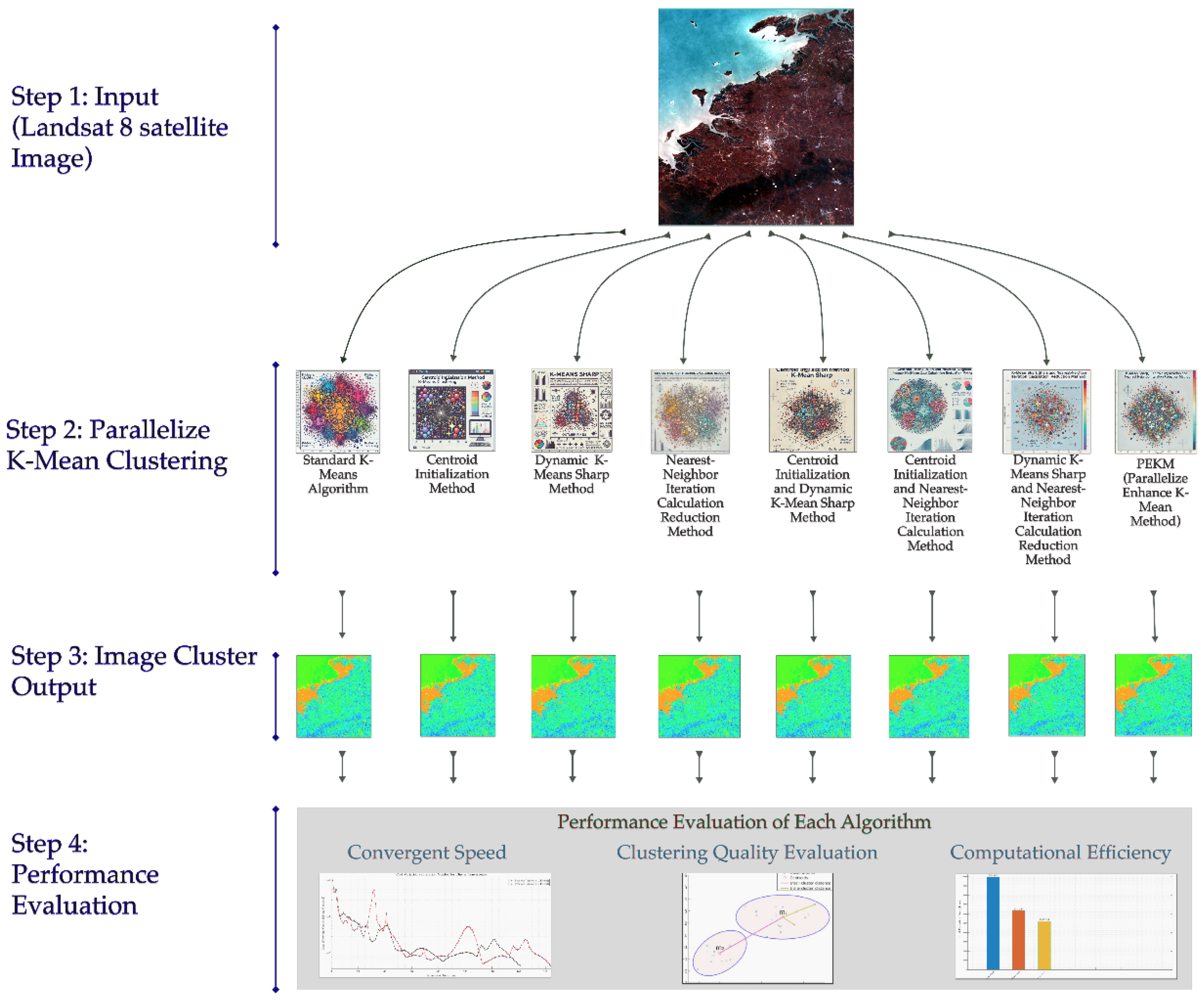
Figure 2.
Selected Dataset Around the world.
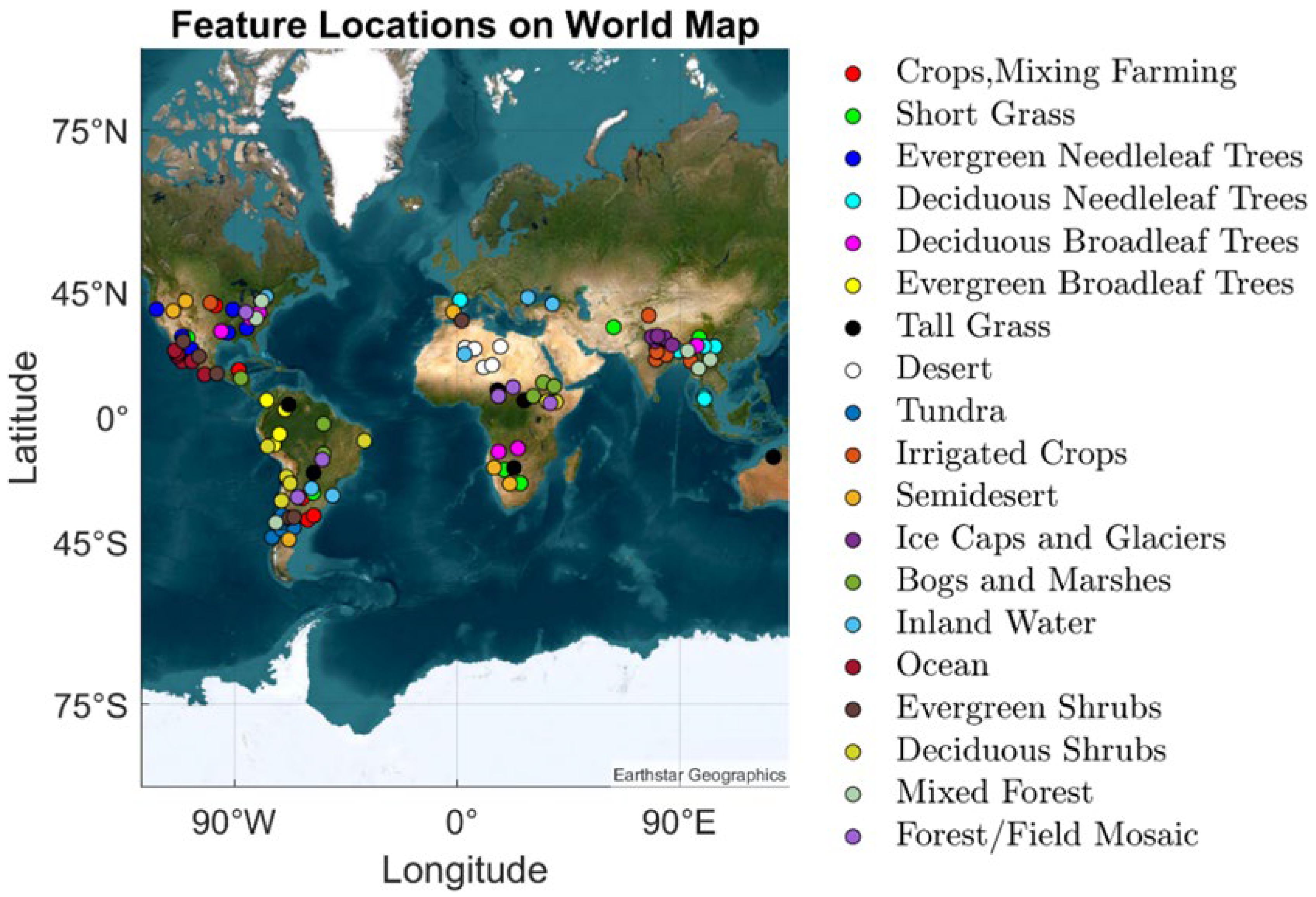
Figure 3.
Job Submission and Execution Pipeline in an HPC Environment.
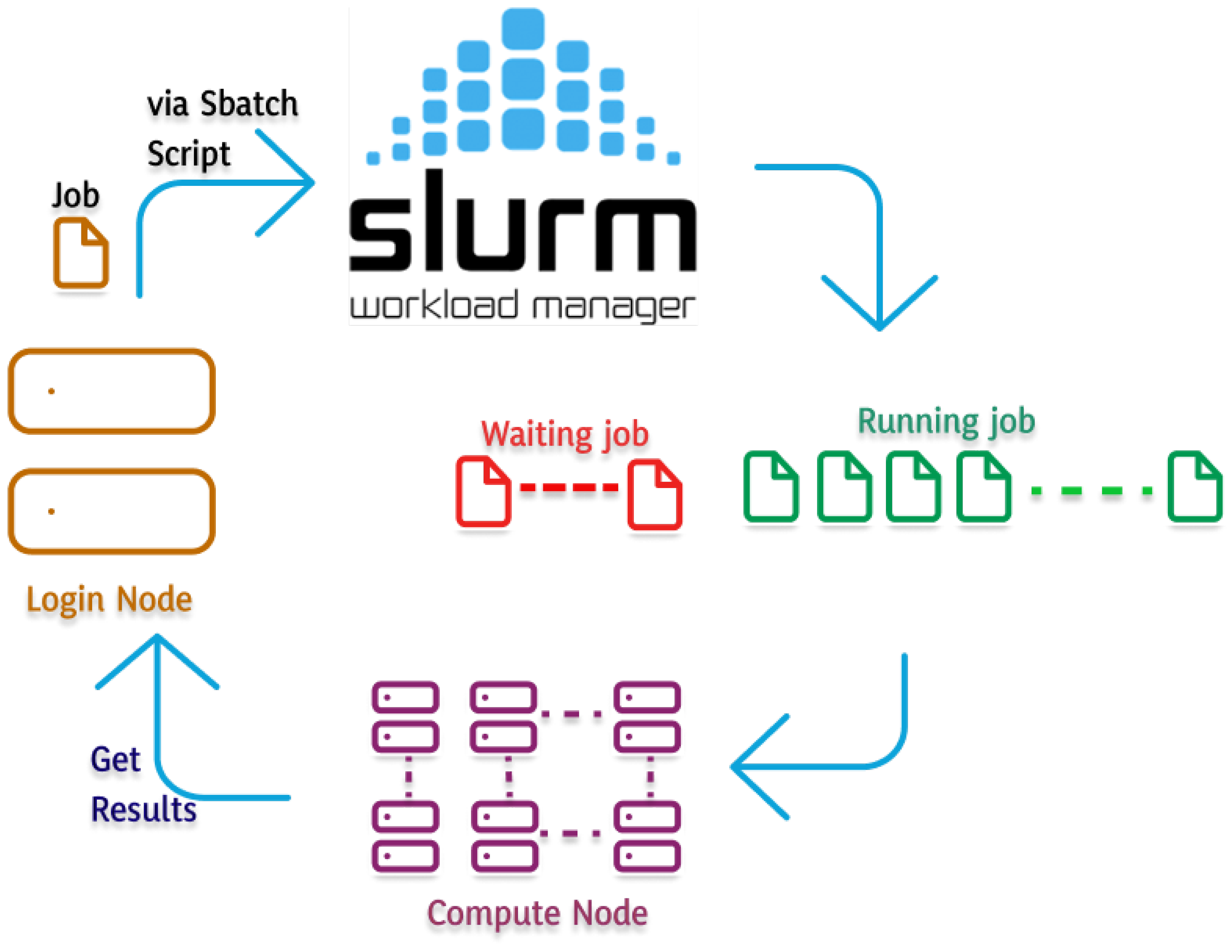
Figure 4.
Operational Flowchart of Parallelization.
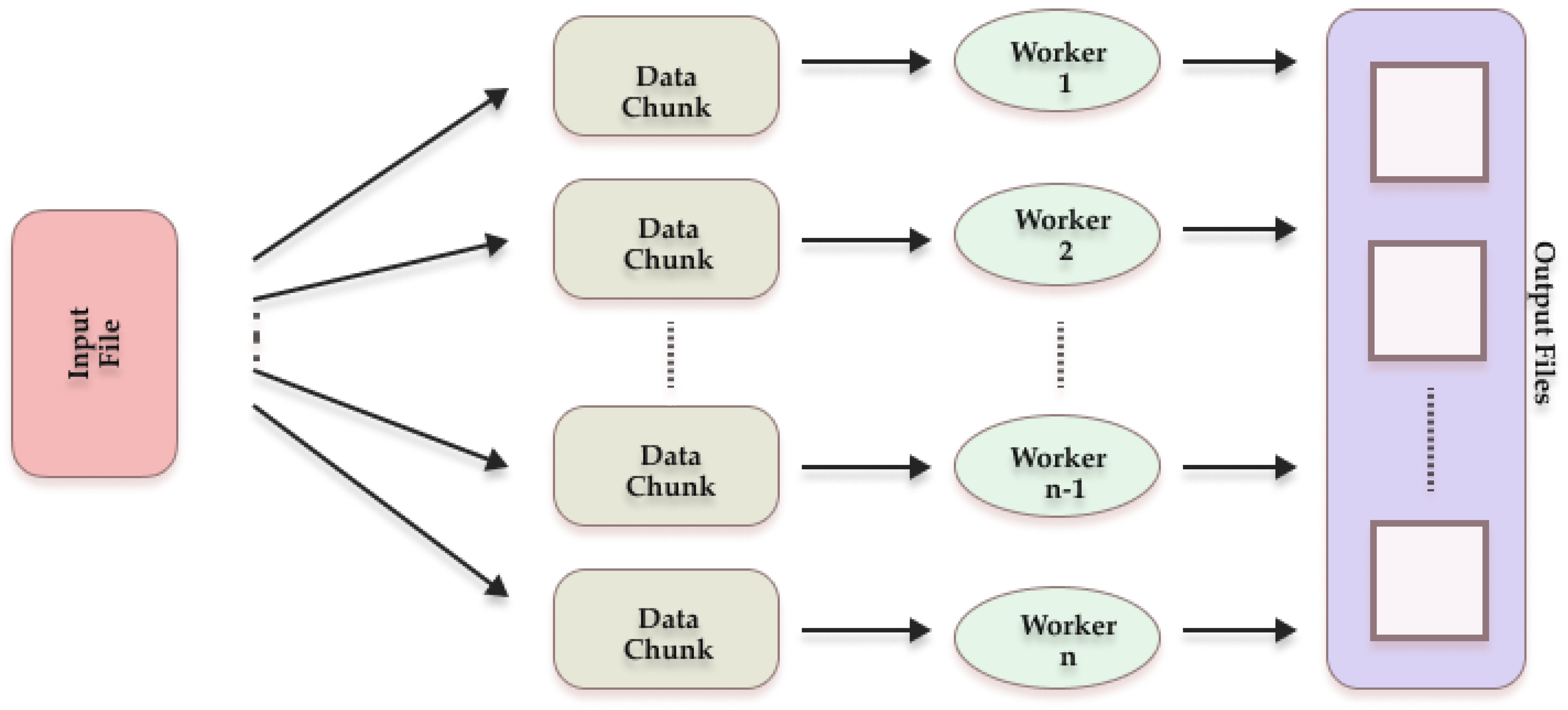
Figure 5.
Cost Variation per Iteration for different Parallelized K-Means Variants.
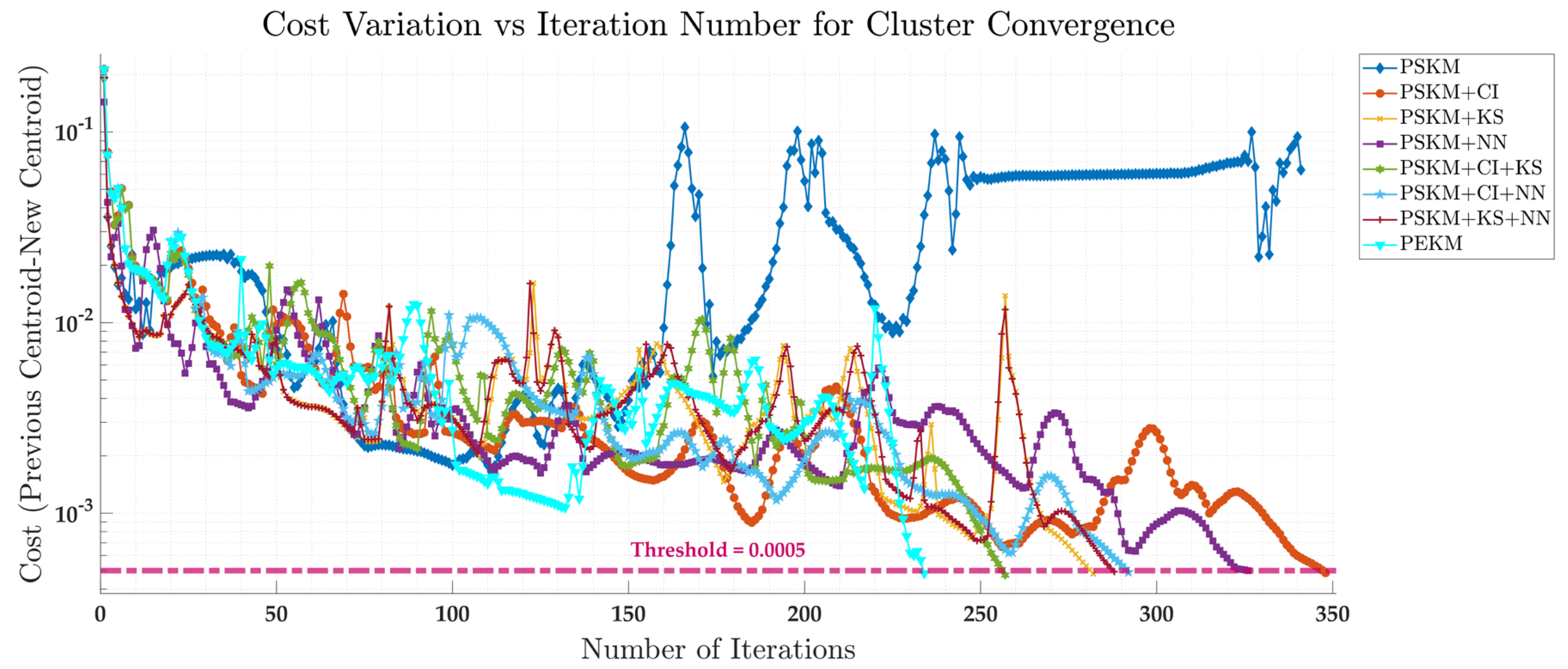
Figure 6.
Bar Plot of Computational Efficiency Comparisons in terms of time.
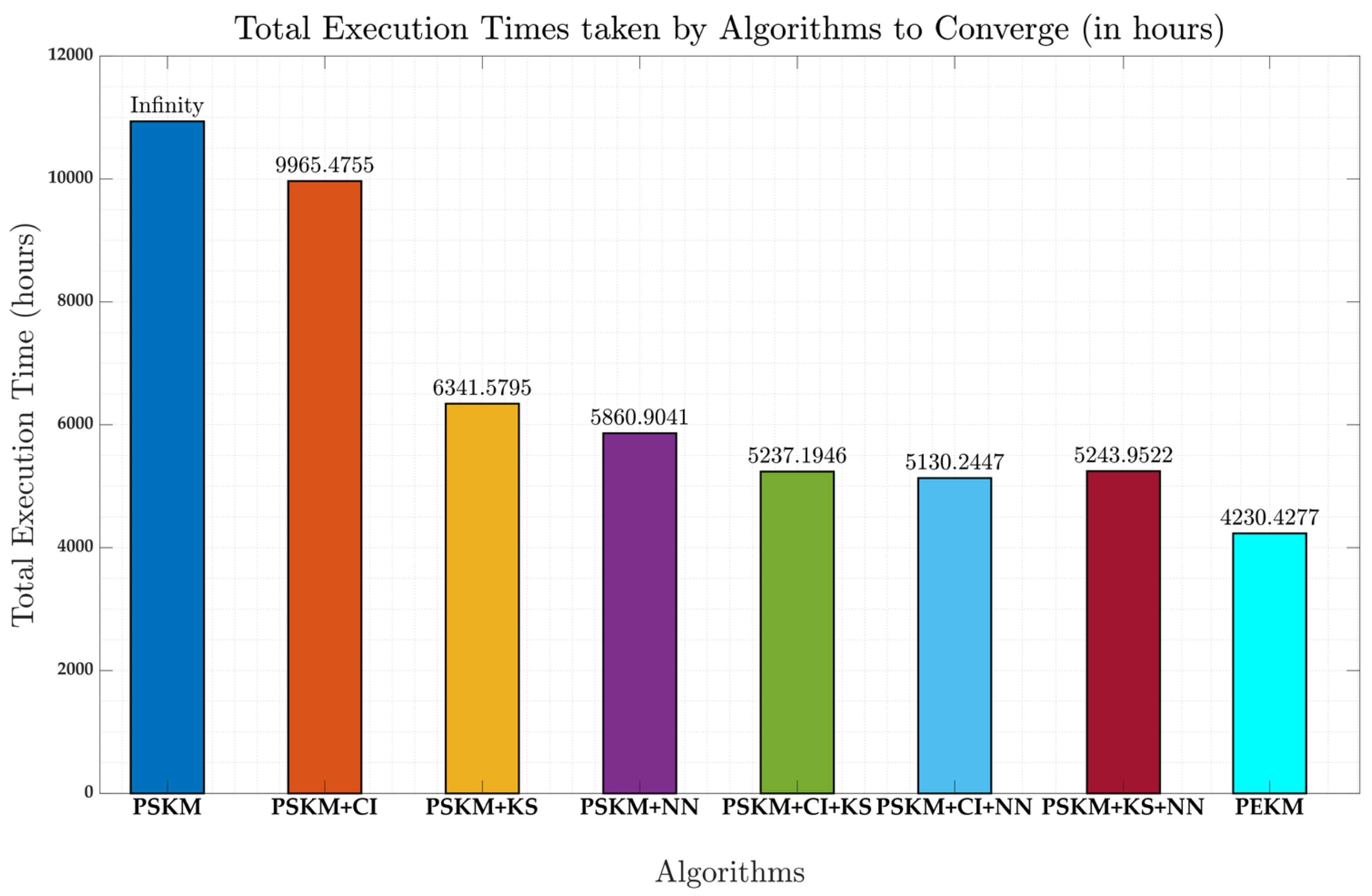
Figure 7.
Bar Plot Cluster Quality Comparison in terms RMSE.
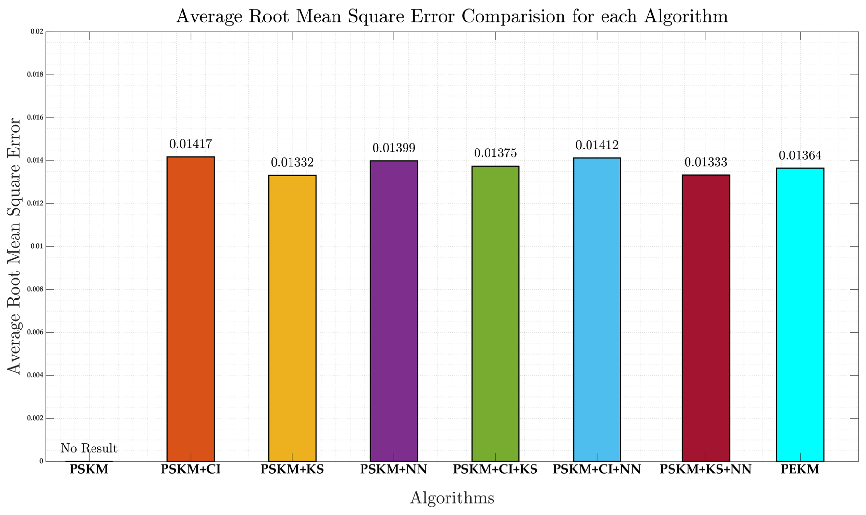
Figure 8.
Cluster-based Masked Image of "Sand" Generated from Parallelized modified K-Means Cluster: (a) Input Image (b) from Parallelized Centroid Initialization method (Reference) (c) Pixel difference between Reference and Parallelized Dynamic K-Means Sharp Method (d) Pixel difference between Reference and Parallelized Nearest-Neighbor Iteration Calculation Reduction Method (e) Pixel difference between Reference and Parallelized Centroid Initialization and Dynamic K-Means Sharp Method (f) Pixel difference between Reference and Parallelized Centroid Initialization and Nearest-Neighbor Iteration Calculation Reduction Method (g) Pixel difference between Reference and Parallelized Dynamic K-Means Sharp and Nearest-Neighbor Iteration Calculation Reduction Method (h) Pixel difference between Reference and PEKM.
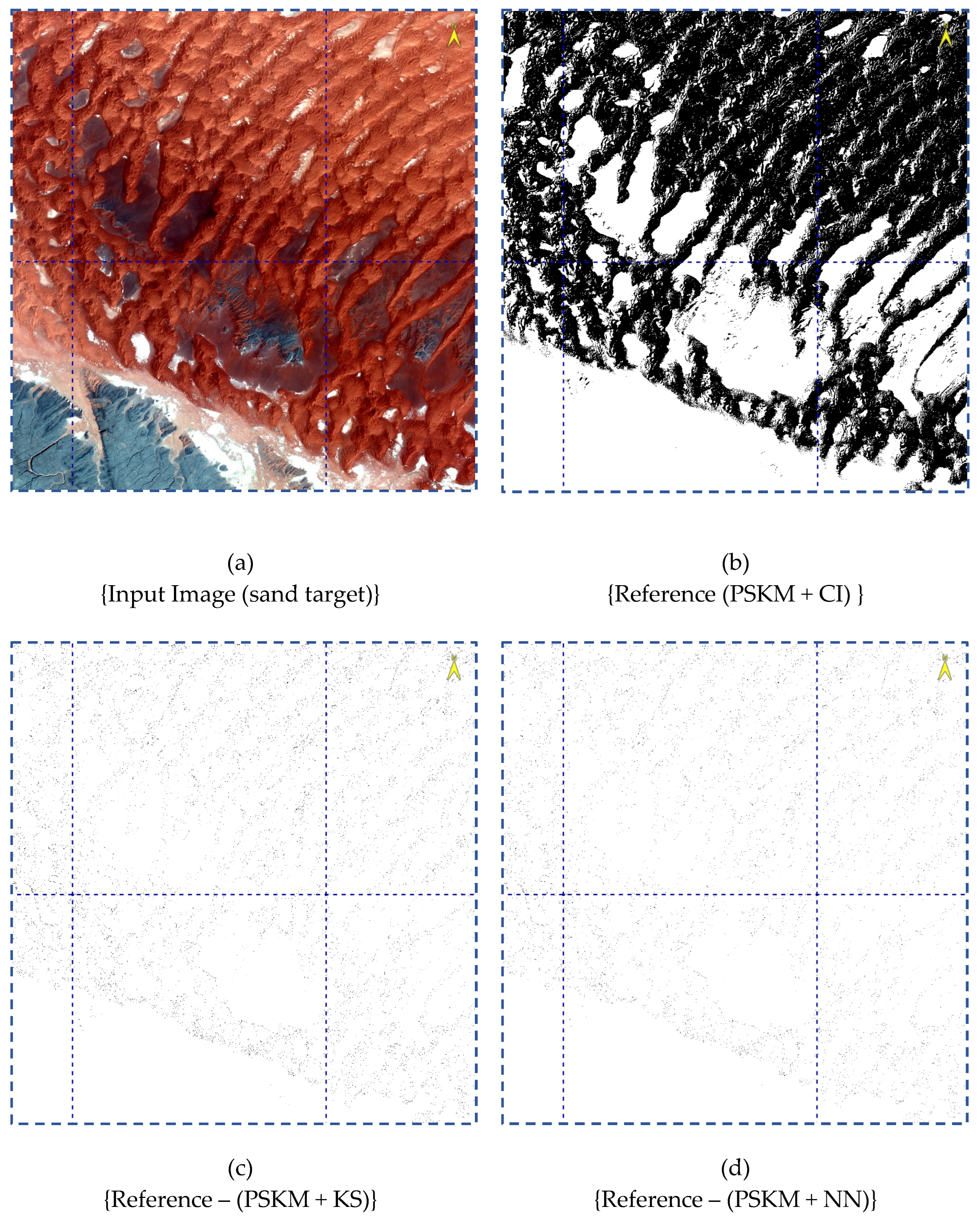
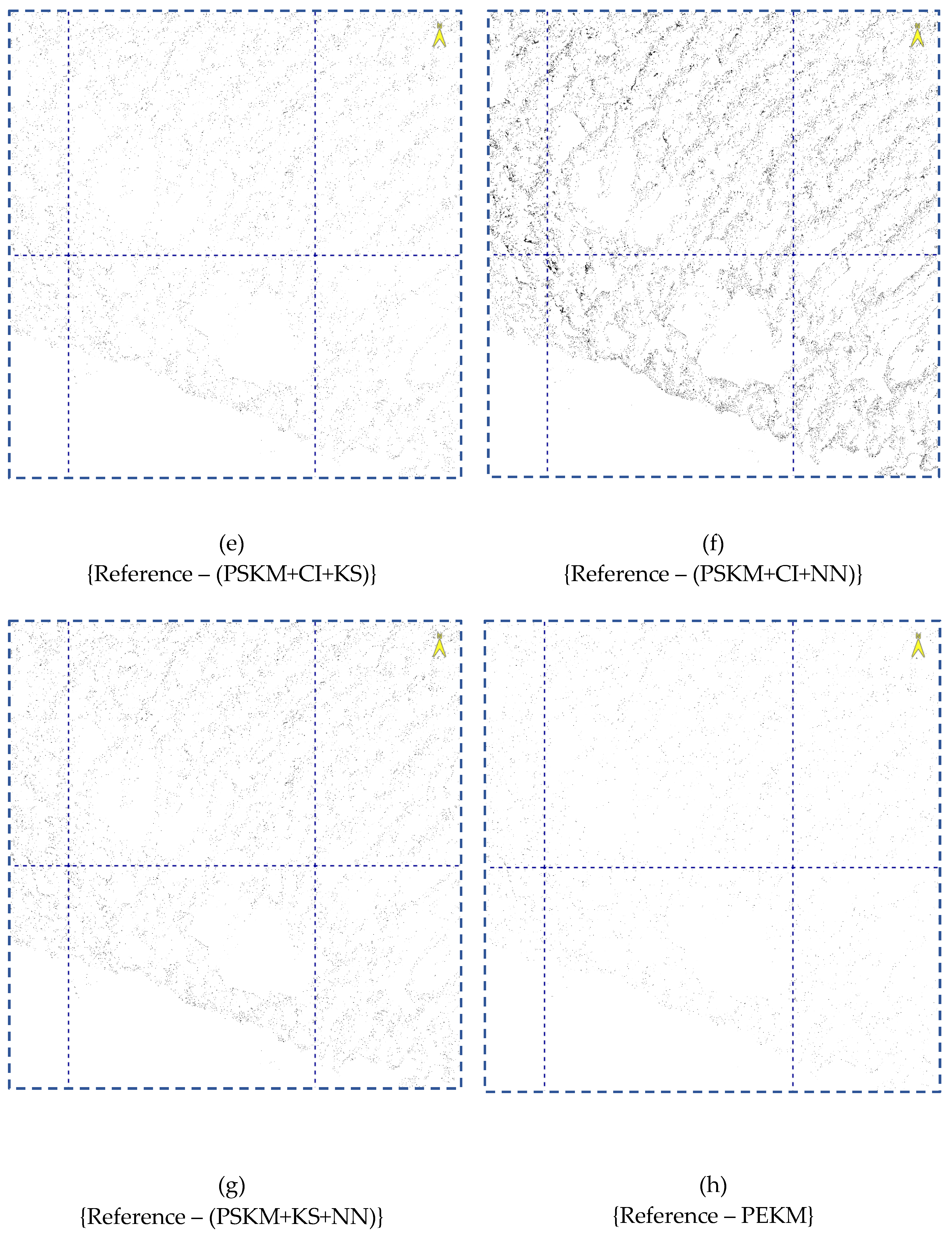
Disclaimer/Publisher’s Note: The statements, opinions and data contained in all publications are solely those of the individual author(s) and contributor(s) and not of MDPI and/or the editor(s). MDPI and/or the editor(s) disclaim responsibility for any injury to people or property resulting from any ideas, methods, instructions or products referred to in the content. |
© 2025 by the authors. Licensee MDPI, Basel, Switzerland. This article is an open access article distributed under the terms and conditions of the Creative Commons Attribution (CC BY) license (http://creativecommons.org/licenses/by/4.0/).
Copyright: This open access article is published under a Creative Commons CC BY 4.0 license, which permit the free download, distribution, and reuse, provided that the author and preprint are cited in any reuse.


