
Submitted:
10 June 2025
Posted:
12 June 2025
Read the latest preprint version here
Abstract
In industries like telecommunications and banking, where labeled data is scarce and mispredictions cost millions, semi-supervised learning (SSL) and active learning (AL) offer promising solutions but often falter due to overconfident predictions, redundant sampling, and inflexible pseudo-labeling thresholds. Traditional approaches tackle these issues separately, limiting their effectiveness in dynamic, real-world settings. This paper introduces a scalable SSL framework called AdaptiveSSL that integrates Wasserstein distance for uncertainty calibration, multi-resolution hashing for efficient diversity-driven sample selection, and Lagrangian optimization for adaptive pseudo-labeling thresholds. By iteratively refining confidence estimates, ensuring representative sampling, and dynamically adjusting thresholds, our system achieves robust churn prediction with AUC scores up to 0.9326, outperforming conventional SSL and AL methods by up to 10%, while maintaining execution times under 90 seconds on large datasets. Tested across four real-world churn datasets, this framework delivers a practical, industry-ready tool for data-efficient classification, paving the way for broader adoption in resource-constrained expert systems.
Keywords:
semi-supervised learning
; adaptive calibration
; pseudo-Labeling
; diversity sampling
; threshold optimization
1. Introduction
The past decade has seen an unprecedented surge in digital data, reshaping domains such as healthcare, finance, autonomous systems, and social media. This wealth of information, however, comes with a persistent challenge: the limited availability of high-quality labeled data. Manual annotation, widely regarded as the benchmark for accuracy, is expensive, labor-intensive, and difficult to scale—particularly in applications like customer churn prediction, where failing to identify at-risk clients can result in significant financial losses. In contrast, unlabeled data, generated effortlessly through automated systems, presents a vast and largely untapped resource. This imbalance has catalyzed the development of semi-supervised learning (SSL) and active learning (AL), two complementary strategies designed to optimize data use while minimizing human intervention.
SSL enhances model performance by integrating a small pool of labeled data with a much larger collection of unlabeled data, capitalizing on the structural insights embedded within the latter [1]. Active learning, by contrast, focuses on identifying and labeling the most informative samples from the unlabeled pool. Recent innovations, such as incorporating self-supervised learning into SSL frameworks, have demonstrated potential in reducing reliance on labeled data by improving the quality of pseudo-labels [2]. Despite these advances, both paradigms encounter significant hurdles that constrain their effectiveness in practical settings. Modern machine learning models, especially deep neural networks, frequently exhibit overconfidence in their predictions, even when uncertainty is high, leading to flawed uncertainty estimates that undermine self-training and pseudo-labeling processes [1]. Additionally, conventional uncertainty-based sample selection often prioritizes redundant examples, limiting the model’s ability to generalize across diverse data distributions. Compounding these issues, static pseudo-labeling thresholds fail to adapt to shifts in data characteristics or model performance during training.
To overcome these limitations, we introduce a semi-supervised framework that integrates three key advancements: dynamic threshold optimization, diversity-promoting sample selection, and adaptive calibration. This approach iteratively refines pseudo-label accuracy and model confidence, drawing inspiration from prior pseudo-labels generated through self-supervised learning [2]. By addressing the shortcomings of isolated and inflexible methods, our framework offers a robust and adaptable solution tailored to the complexities of real-world environments.
1.1. Motivation and Problem Definition
The impetus for this research stems from the pressing need to leverage unlabeled data in applications where errors carry substantial consequences—such as retaining customers in telecommunications or ensuring accurate diagnoses in healthcare. In these high-stakes contexts, traditional supervised models often produce predictions with unwarranted confidence, even under uncertain conditions, which propagates errors when these predictions are repurposed as pseudo-labels. This instability not only degrades performance but also erodes trust in the training process. Furthermore, existing SSL techniques, which rely heavily on uncertainty estimates for sample selection, tend to focus on a narrow subset of ambiguous cases, repeatedly choosing similar examples while overlooking the broader data landscape. This selective bias hampers generalization. Static or heuristically set pseudo-labeling thresholds exacerbate the problem, as they cannot adjust to the evolving quality of predictions, allowing low-quality pseudo-labels to persist and amplify errors over time.
Our framework seeks to address these challenges through a cohesive strategy anchored in three objectives:
- Dynamic Prediction Calibration: Implement a mechanism to continuously refine confidence estimates, ensuring they align with true uncertainty and mitigate overconfidence.
- Diverse Sample Selection: Employ methods to select unlabeled samples that reflect the full spectrum of the data distribution, preventing redundancy and enhancing representativeness.
- Adaptive Pseudo-Labeling Thresholds: Develop a system that adjusts thresholds in real-time based on model performance, maintaining the integrity of pseudo-labels throughout training.
By uniting these elements, our approach fosters a resilient learning system capable of harnessing both labeled and unlabeled data to improve accuracy and robustness.
1.2. Advances and Limitations in Semi-Supervised Learning
Recent progress in SSL underscores the power of combining small labeled datasets with extensive unlabeled ones to boost accuracy and generalization [1]. Early SSL methods assumed that labeled and unlabeled data originated from the same underlying distribution—a premise that often does not hold in real-world scenarios, such as medical imaging, where patient characteristics and image quality vary widely [3]. Contemporary deep learning models, despite their sophistication, frequently generate overconfident outputs, skewing uncertainty estimates and complicating self-training processes that depend on pseudo-labels [4]. Calibration techniques like temperature scaling have been employed to address this, but they lack the flexibility to adapt to shifting data distributions.
Active learning has similarly evolved, reducing the demand for labeled samples by prioritizing those with high uncertainty, often measured via entropy or margin sampling. Yet, these strategies tend to select redundant samples, failing to capture the diversity of the data [5]. Recent efforts have introduced adaptive thresholding to refine selection [6], though diversity remains a secondary consideration. Complementary research on uncertainty estimation and noise mitigation [7,8] has deepened our understanding of SSL and AL, but these studies typically explore issues in isolation rather than within a unified framework. Meanwhile, semi-supervised transfer boosting demonstrates that dynamic thresholding, guided by real-time model evaluation, can curb error propagation [9], highlighting the value of adaptability.
1.3. Integrating Advances Across Domains
Emerging trends in machine learning emphasize the interconnected nature of SSL and AL challenges, suggesting that a holistic approach can unlock synergies between calibration, diversity, and thresholding. For instance, Sohn et al. [10] proposed a dynamic pseudo-labeling strategy that adjusts thresholds based on ongoing performance, underscoring the importance of adaptability. Berthelot et al. [11] combined multiple techniques to tackle both calibration and sample diversity, paving the way for more integrated solutions. In graph classification, semantic prototypes and subgraph-level uncertainties enhance the handling of unlabeled data [12], refining calibration and providing supervision for unknown classes. Qu et al. [13] developed a thresholding method that adjusts confidence levels according to class frequencies, improving reliability in imbalanced datasets, while Ji et al. [14] integrated mutual information and error reduction for diverse sample selection. Advances in domain adaptation, such as joint Wasserstein distance minimization, further stabilize pseudo-labels under distribution shifts [15], bolstering SSL’s robustness in dynamic contexts.
1.4. Comprehensive Comparison with Recent Studies
Zhou et al. [3] demonstrated that fixed pseudo-labeling thresholds struggle with the variability of medical imaging data, leading to suboptimal outcomes in tasks like brain lesion segmentation. Xie et al. [16] found that self-training frameworks suffer from accumulating errors due to poor pseudo-labels, reinforcing the need for adaptive mechanisms. Minderer et al. [4] highlighted how overconfident predictions undermine uncertainty reliability, prompting the development of dynamic calibration methods. Ash et al. [5] noted that uncertainty-based AL often selects redundant samples, limiting data coverage. Contributions from Rizve et al. [6], Xia et al. [7], and Li et al. [8] offer insights into uncertainty and noise management, yet their fragmented approaches fall short of addressing SSL and AL’s multifaceted challenges. Sohn et al. [10] and Yu et al. [17] advance dynamic thresholding, but often as auxiliary rather than core components. Our framework builds on these findings, integrating adaptive calibration, diversity, and thresholding into a unified system.
1.5. Identified Gaps and Unresolved Challenges
Despite significant strides, SSL and AL face ongoing obstacles:
- Static Pseudo-Labeling Thresholds: Fixed thresholds fail to adjust to changes in data quality or distribution, incorporating unreliable pseudo-labels.
- Overconfident Predictions: Models overestimate certainty, propagating errors through pseudo-labels.
- Redundant Sample Selection: Uncertainty-driven methods select similar examples, neglecting data diversity.
- Fragmented Approaches: Calibration, diversity, and thresholding are often treated separately, limiting their combined potential.
- Insufficient Adaptability: Static strategies struggle with evolving data distributions, reducing effectiveness over time.
- Scalability and Efficiency: Computationally intensive methods hinder applicability to large-scale problems.
Resolving these gaps is critical for deploying SSL and AL in real-world settings.
1.6. Synthesis of Contributions and Novel Framework
Our proposed framework addresses these challenges with a unified, adaptive system:
- Adaptive Calibration and Reliable Uncertainty Estimation: A reweighting mechanism, leveraging Wasserstein temperature scaling and cross-validation, refines confidence estimates to reflect true uncertainty, reducing overconfidence risks [15].
- Diversity-Promoting Sample Selection: A linear-time sampler using multi-resolution hashing ensures selected samples represent the full data distribution, avoiding redundancy.
- Dynamic Threshold Optimization: A Lagrangian-based optimizer adjusts pseudo-labeling thresholds based on real-time performance, minimizing error propagation.
- Scalability and Integration: Efficient design enables scaling to large datasets, with each component enhancing the others’ effectiveness.
This framework not only overcomes individual limitations but also delivers a robust, adaptable solution for diverse, evolving data landscapes.
1.7. Structure of the Paper
The remainder of the paper is structured as follows. In Section 2, we introduce the proposed model, explaining its key components and methodologies in detail. Section 3 provides an overview of the datasets used, along with data preprocessing and feature engineering techniques. In Section 4 and Section 5, we present extensive experimental results, comparing our approach with several baseline models, discusses the computational efficiency of the proposed framework and conducting an ablation study to assess the contribution of individual components. Section 6 provides a statistical comparison of the proposed model against various baselines, incorporating multiple statistical tests and performance analysis techniques, including conditional entropy distribution and ROC curves. Finally, Section 7 concludes the paper by summarizing the key findings, discussing limitations and outlining potential directions for future research.
2. Proposed Model
In this paper, we introduce an integrated semi-supervised learning framework called AdaptiveSSL that combines adaptive probability calibration, diversity-promoting sampling and dynamic pseudo-label threshold optimization into a unified iterative process. The primary objective is to enhance classifier performance by effectively incorporating large-scale unlabeled data into the training procedure. In the following subsections, we describe each component of the framework in detail and compare the proposed approach with multiple alternative methods to justify our design choices.
2.1. Base Classifier: LightGBM
The base classifier chosen for this framework is LightGBM (Light Gradient Boosting Machine) [18], a gradient boosting decision tree method. Let denote the mapping performed by the classifier, where d is the dimensionality of the input space and K is the number of classes. For an input sample , the classifier outputs a probability vector
with . LightGBM is selected due to its lightweight structure, fast training speed, and low memory consumption. These properties are crucial when processing large datasets and performing multiple iterations in a semi-supervised context. In contrast to more complex deep models, LightGBM achieves competitive performance with fewer computational resources, making it well-suited for iterative pseudo-labeling procedures [19]. Furthermore, LightGBM incorporates L1 and L2 regularization to prevent overfitting, which is crucial in semi-supervised learning where noisy pseudo-labels can exacerbate this issue. Hyperparameters such as n estimators, learning rate, number of leaves and feature fraction are tuned using ROC AUC via a randomized search procedure. We use RandomizedSearchCV in our implementation to efficiently explore the hyperparameter space and identify the configuration that maximizes performance on a validation set [20].
2.2. Adaptive Calibration
Overview: A fundamental challenge in classification models is the tendency to produce overconfident predictions, leading to miscalibration and unreliable uncertainty estimates. To mitigate this issue, we introduce an adaptive calibration framework that systematically adjusts the predicted class probabilities. Our objective is to ensure that the output probabilities align with the true likelihood of each class, thus enhancing the reliability of confidence estimates [21].
Our approach consists of two major components:
- Temperature scaling, where the temperature parameter is dynamically adjusted based on an empirical measure of confidence dispersion.
- Post-hoc calibration using cross-validation via Calibrated Classifier, which ensures robustness against overfitting [22].
The complete procedure is outlined in Algorithm 1.
| Algorithm 1 Adaptive Calibration |
|
Mathematical Formulation:
For an input , the classifier produces a probability vector , where represents the predicted probability of class k. We define the confidence score as:
Let denote the set of unlabeled samples, and define their corresponding confidence scores as . Sorting these confidence scores in ascending order yields the ordered sequence .
To measure the deviation between this empirical confidence distribution and a perfectly uniform distribution, we introduce the uniform quantile sequence:
The discrepancy between these distributions is quantified using the empirical Wasserstein distance [23]:
Theoretical Justification: The Wasserstein distance is selected for its ability to capture both the magnitude and structural shifts in the distribution of confidence scores. This dual sensitivity ensures that even subtle calibration mismatches—indicative of overconfident or underconfident predictions—are effectively quantified as formalized in [24]. In our framework, this property directly informs the adaptive temperature parameter:
which scales with both the confidence dispersion and the number of classes K, thus preventing excessive smoothing while properly adjusting for uncertainty.
2.2.1. Comparative Analysis of Distance Metrics
In order to get a deeper insight into why the Wasserstein distance has been selected, the comparison with other popular metrics for distributional similarity measures is provided. Table 1 summarizes the key advantages and disadvantages associated with the Kullback-Leibler (KL) divergence, total variation (TV) distance, Hellinger distance and Wasserstein distance. While the Kullback-Leibler divergence is highly sensitive to distributional shape changes and the total variation distance is straightforward to interpret thanks to being bounded, both measures ignore the spatial organization of confidence scores. The Hellinger distance provides symmetry and demonstrates robustness against tiny fluctuations. however, it is not very successful at capturing the underlying geometric structure. In contrast, the Wasserstein distance naturally unites magnitude and geometric perspectives, which is especially useful for stable calibration.
Hyperparameter Rationale: The factor 2.5 in the temperature equation was determined through empirical validation. Extensive experiments showed that this value provides an optimal balance between calibration sensitivity and stability, ensuring that T remains within a practical range across different datasets. Too high a value would lead to excessive smoothing, whereas a lower value would limit adaptivity.
Once the temperature is set, the calibrated probabilities are obtained via temperature scaling [25]:
Finally, uncertainty is quantified using Rényi entropy of order 2 [26]:
Rényi entropy is particularly useful as it amplifies differences in high-confidence regions, providing a more informative measure of predictive uncertainty.
2.2.2. Rationale and Comparison: Adaptive Calibration
The proposed adaptive calibration mechanism overcomes the limitations of traditional static methods by dynamically adjusting the temperature parameter based on the empirical confidence distribution. Additionally, we incorporate CalibratedClassifierCV from scikit-learn [27] with a 2-fold cross-validation strategy to further improve reliability. The 2-fold configuration ensures that the calibration model is trained on separate data partitions, reducing overfitting and enhancing generalization. Table 2 provides a comparative analysis of various calibration methods.
As illustrated in Table 2, while methods such as isotonic regression offer high robustness, they lack adaptivity over iterations. Our proposed method, which combines dynamic temperature scaling with cross-validation, achieves both adaptivity and high robustness. Robustness here refers to the method’s ability to maintain calibration performance even in the presence of noisy data or model misspecification.
The workflow of adaptive calibration is illustrated in Figure 1. The diagram provides a step-by-step visualization, emphasizing the Wasserstein-based temperature adjustment and entropy-based uncertainty estimation.
2.3. Diversity-Promoting Sampling
After calibration, to ensure that the selected pseudo-labeled samples are representative of the broader unlabeled data distribution, we employ a diversity-promoting sampling strategy based on the Linear Diversity Sampler [28]. This method aims to select a diverse subset of samples with approximately complexity, where n is the number of unlabeled samples. The steps of the Linear Diversity Sampler are outlined in Algorithm 2.
| Algorithm 2 Diversity-Promoting Sampling |
|
The Linear Diversity Sampler leverages several techniques to achieve efficient and effective diversity sampling:
-
Dimensionality Reduction with SVD: Initially, Singular Value Decomposition (SVD) [29] is applied to reduce the dimensionality of the unlabeled data. Specifically, we compute the truncated SVD of the data matrix , approximating it aswhere is a matrix of left singular vectors, is a diagonal matrix of singular values, and is a matrix of right singular vectors. We then project the data into a lower-dimensional subspace by computingThe rank k is set to approx_rank, dynamically adjusted to be no larger than to ensure a valid decomposition. This step reduces the computational cost of subsequent hashing operations and captures the principal components of the data.
-
Multi-Resolution Hashing: After dimensionality reduction, multi-resolution hashing [30] is performed to capture diversity at multiple scales. The reduced data is scaled by geometric factors of 0.5, 1.0, and 2.0, resulting in:For each scaled version, random hyperplanes are generated. Each hyperplane is defined by a normal vector , sampled from a normal distribution and normalized by dividing by its norm:The partition code for a data point is given bywhich yields a binary code [31]. This process generates a set of binary partition codes for each data point at each resolution.
- Unique Hash Selection: The binary partition codes from all scaling factors are horizontally stacked and converted to integers. A unique hash for each data point is computed by applying a hash function (e.g., Python’s built-in hash function) to the tuple of concatenated binary codes. These unique hash values are then used to identify a set of unique samples.
- Fallback Mechanism: In cases where the number of unique hashes is below the target sample size, a fallback mechanism is employed. Specifically, the sampler randomly selects additional samples from the unlabeled data until the desired number of samples is reached. This ensures that the diversity sampler always returns exactly T samples.
The computational complexity of the Linear Diversity Sampler is approximately due to the efficiency of the truncated SVD and the linear-time operations involved in multi-resolution hashing and unique hash selection. The diversity of the selected samples ensures that the model is exposed to a wide range of data patterns, which can improve its generalization ability.
2.3.1. Rationale and Comparison: Diversity Sampling
Table 3 provides a comparison of our proposed multi-resolution hashing method with several alternative diversity sampling approaches.
As illustrated in Table 3, our multi-resolution hashing method achieves a balance between scalability and diversity. While DPP-based sampling offers excellent diversity guarantees, its cubic complexity makes it unsuitable for large-scale scenarios [32]. In contrast, clustering-based approaches and random sampling either lack robustness or explicit diversity control. Our method, with linear scalability (excluding the SVD step), is practical for large datasets while ensuring competitive diversity.
Figure 2 illustrates the workflow of the diversity-promoting sampling component.
2.4. Dynamic Threshold Optimization
Following the diversity-promoting sampling process, which ensures that the pseudo-labeled samples are representative of the broader unlabeled data distribution, we further refine the pseudo-labeling by dynamically optimizing the threshold using an adaptive Lagrangian formulation [33]. Determining the optimal pseudo-label threshold is critical for balancing precision and recall. We frame threshold selection as an optimization problem, where the objective is defined as a weighted combination of performance metrics, and solve it using a ternary search algorithm [34] combined with adaptive Lagrangian multiplier updates. In our implementation, the performance targets for both score and recall are implicitly set at 0.8, and the Lagrangian multipliers are updated accordingly based on an adaptivity factor.
2.4.1. Lagrangian Formulation
Let and denote the F1 score and recall at threshold t, respectively. In our approach, we define an objective function as the negative weighted sum of key performance metrics:
where is Youden’s J-statistic [35] and is the G-mean [36]. The weights are selected based on empirical studies to prioritize overall balance and discrimination ability. While the formulation may be viewed as implicitly enforcing performance targets (with and expected to exceed 0.8), the adaptive update of Lagrangian multipliers further guides the threshold toward the desired operating point.
The Lagrangian multipliers and are updated as follows:
Adaptivity Factor:
The adaptivity factor is a step-size parameter that controls the magnitude of adjustments made to the Lagrangian multipliers during the optimization process. In our implementation, we set the adaptivity factor to 0.1. This means:
- If or is below the target of 0.8, the corresponding multiplier is increased by 10% (i.e., multiplied by ).
- Conversely, if the metric meets or exceeds 0.8, the multiplier is decreased by 10% (i.e., multiplied by ).
This choice of 0.1 was determined empirically to balance responsiveness to performance deficits with the overall stability of the threshold optimization process.
2.4.2. Ternary Search and Adaptive Updates
The optimal threshold is determined using a ternary search over the interval . Ternary search is particularly efficient for unimodal functions and converges in
iterations, where (e.g., ) is the tolerance [37]. The algorithm evaluates two internal points within the search interval, updates the interval based on the objective function comparison, and iterates until convergence. Once the threshold is optimized, the adaptive Lagrangian multipliers are updated based on the observed and recall, ensuring that the search process remains sensitive to the classifier’s performance [38].
2.4.3. Algorithm and Workflow
Algorithm 3 details the dynamic threshold optimization procedure, while Figure 3 presents a workflow that distinctly captures the iterative and adaptive aspects of the process.
| Algorithm 3 Dynamic Threshold Optimization |
|
2.4.4. Rationale and Comparison: Dynamic Threshold Optimization
Ternary Search: Ternary search is employed because the objective function is observed to be unimodal within the search interval [37]. Unlike grid search, which requires exhaustive evaluation of many points, ternary search efficiently narrows down the optimal threshold by evaluating only two intermediate points per iteration. This reduces the computational cost to , where is the tolerance level. Such efficiency is crucial in iterative active learning frameworks where threshold optimization is performed repeatedly [39].
Lagrangian Formulation: The Lagrangian formulation allows us to combine multiple performance metrics (i.e., , precision, recall, Youden’s J-statistic, and G-mean) into a single scalar objective while implicitly enforcing performance targets [40]. By incorporating Lagrangian multipliers and , we can adaptively penalize deviations from desired levels (set at 0.8 in our case) for and recall, respectively. This formulation not only guides the optimization toward a balanced operating point but also provides a systematic way to adjust the threshold in response to fluctuations in model performance [40]. The adaptive update of these multipliers, based on an adaptivity factor, further enhances the robustness of the threshold optimization process.
Table 4 also compares our proposed dynamic threshold optimization with several alternative pseudo-label thresholding methods.
As illustrated in Table 4, our dynamic threshold optimization method, which employs a ternary search algorithm combined with adaptive Lagrangian multiplier updates, not only adapts to changes in classifier performance but does so with high robustness and efficiency. While grid search and Bayesian optimization can also optimize thresholds, they either lack adaptivity or impose a higher computational burden. Our approach strikes an effective balance between adaptivity, robustness, and computational cost.
2.5. Integrated Iterative Framework
Overview: The three components described above are integrated into an iterative semi-supervised learning framework. In each iteration, the classifier is retrained using the expanded labeled set, and new pseudo-labels are generated from the unlabeled data. The overall process is as follows:
- Classifier Training: Train the LightGBM classifier using the current labeled dataset .
- Prediction: Compute the prediction probabilities for each sample .
- Calibration: Apply the adaptive calibration procedure (Algorithm 1) to obtain calibrated probabilities and uncertainty estimates .
- Uncertainty-Based Selection: Identify samples with high uncertainty (as measured by ).
- Diversity Selection: From the uncertain samples, select a diverse subset using the multi-resolution hashing method (Algorithm 2).
- Threshold Optimization: Determine the optimal pseudo-labeling threshold via dynamic threshold optimization (Algorithm 3).
- Pseudo-Labeling: Assign pseudo-labels to samples in that satisfy .
- Dataset Update: Augment with the newly pseudo-labeled samples and remove these samples from .
- Iteration: Repeat the process until a stopping criterion is met (e.g., when falls below a predefined size).
| Algorithm 4 Iterative Semi-Supervised Learning Framework |
|
Figure 4 provides an overall diagram of the iterative framework.
2.6. Computational Complexity Analysis
The proposed framework is designed with efficiency in mind. The computational cost of each component is analyzed as follows:
- Adaptive Calibration: Sorting the confidence scores requires time, and subsequent temperature scaling and entropy computations operate in .
- Diversity Sampling: The truncated SVD has complexity , where r is significantly smaller than d. The multi-resolution hashing itself is computed in .
- Dynamic Threshold Optimization: The ternary search converges in iterations, with each iteration evaluating the objective function in constant time.
Thus, the overall complexity is dominated by the sorting and SVD operations, ensuring scalability for large datasets.
Summary
In summary, the proposed model is an integrated semi-supervised learning framework that leverages adaptive calibration, diversity-promoting sampling, and dynamic threshold optimization to improve the quality of pseudo-labeling. Each component is rigorously formulated with precise mathematical notations, and detailed comparisons with alternative methods are provided via tables. The integration with a lightweight yet effective LightGBM classifier ensures both high performance and scalability for large-scale applications.
3. Dataset Information, Preprocessing, and Feature Engineering
3.1. Dataset Selection Rationale
Four binary classification based customer churn based datasets were selected to evaluate model performance across data scales and structural complexities. These datasets include a large-scale streaming behavior dataset (Sparkify), a structured telecommunications dataset (IBM Telco), a banking dataset capturing financial churn (Bank Churn), and a high-dimensional service dataset (CrowdAnalytix). Table 5 summarizes their key attributes and selection rationale.
3.2. Dataset Information
3.2.1. Sparkify Dataset
The Sparkify dataset [41] is a 12.5GB JSON file containing 26,259,199 user interaction records over a three-month period (Oct–Dec 2018) with 18 features. It includes 12 categorical (e.g., userId, gender, auth, page) and 6 numerical columns (e.g., sessionId, length, itemInSession). Churn is defined as users who clicked the "Cancel Confirmation" button, resulting in 5,003 (22.45%) churned users. Preprocessing involved flattening the nested JSON structure, handling missing values, and session-based feature extraction.
3.2.2. IBM Telco Dataset
The IBM Telco dataset [42] consists of 7,043 customer records merged from three sources: customer status, demographics, and service usage. It originally contained 48 features, but 12 were dropped due to redundancy, leaving 36. Key attributes include contract type (monthly, one-year, two-year), payment method, tenure, and security services. Churn prediction is strongly influenced by contract length, service subscriptions, and monthly charges. The dataset has a churn rate of 26.5%. Feature selection was performed using mutual information, with top contributing features including contract type, tenure, total charges, and online security.
3.2.3. Bank Churn Dataset
The Bank Churn dataset [43] contains financial information for 10,000 customers across France, Germany, and Spain. It has 14 raw features, including credit score, balance, number of products, and estimated salary. One-hot encoding of categorical variables expanded the dataset to 2,948 dimensions. The churn rate is 20.37% (2,037 churned users). Feature selection based on mutual information identified NumOfProducts, Age, and IsActiveMember as key predictors.
3.2.4. CrowdAnalytix Dataset
The CrowdAnalytix dataset [44] consists of 51,047 customer records with 58 features, primarily from the telecommunications domain. It contains both numerical and categorical variables relevant to customer behavior, such as MonthlyRevenue, MonthlyMinutes, TotalRecurringCharge, and Call patterns. The dataset also includes demographic and service-related attributes such as Age, Handset models, Credit Rating, and Marital Status.
The churn rate in this dataset is 28.83%, with 14,711 churned users and 36,336 non-churned users. Preprocessing involved handling missing values, encoding categorical variables, and standardizing numerical attributes.
3.3. Data Preprocessing
Preprocessing steps varied across datasets based on structure and challenges:
- Sparkify: Flattened nested JSON, removed users with missing IDs, converted timestamps, and encoded categorical values.
- IBM Telco: Droped irrelevant columns such as Customer ID, Churn Label, Churn Score etc. and also encoded categorical variables using label encoding.
- Bank Churn: Encoded categorical features using one-hot encoding, normalized continuous variables, and dropped irrelevant columns like CustomerId and Surname.
- CrowdAnalytix: Categorical variables were label-encoded, missing numerical values were imputed using mean values, and all features were standardized.
3.4. Feature Engineering
Feature engineering created new predictive variables:
- Sparkify: Session entropy, monthly session duration, average listen time, ad interruptions, and offline listening.
- IBM Telco: Service bundle compatibility score, contract duration bins, and monthly charge volatility.
- Bank Churn: Credit utilization ratio, customer activity score, and tenure-product interaction terms.
- CrowdAnalytix: Derived features such as call behavior metrics (dropped calls, unanswered calls, inbound/outbound ratios), and tenure-based segmentation.
3.5. Feature Selection
A hybrid feature selection strategy was applied to reduce dimensionality:
- IBM Telco: Used Mutual Information [47] to identify 10 key features.
- Bank Churn: Used Mutual Information to identify the top 10 features, which included NumOfProducts, Age and IsActiveMember.
- CrowdAnalytix: Used Mutual Information to identify the top 10 features, which included AgeHH1, DroppedCalls, DroppedBlockedCalls, BlockedCalls and InboundCalls.
3.6. Class Imbalance Handling
3.7. Summary
This study leverages four diverse datasets with varying structures, sizes, and feature spaces to assess model performance across different domains. Each dataset required tailored preprocessing, feature engineering, and feature selection strategies. The Sparkify dataset presented challenges in handling large-scale JSON data, while the IBM Telco and Bank Churn datasets highlighted structured feature selection complexities and class imbalance issues. Additionally, the CrowdAnalytix dataset introduced a high-dimensional feature space, requiring advanced dimensionality reduction techniques. Collectively, these datasets serve as a robust benchmark for evaluating churn prediction models across multiple industries.
4. Experiment and Results
In this section, we present a comprehensive evaluation of our proposed semi-supervised model against several state-of-the-art baseline methods. The experiments were conducted on four real-world datasets described in the above section—Sparkify, IBM Telco, Banking, and CrowdAnalytix—under two scenarios: using 5% and 10% labeled data. Performance was assessed using multiple metrics including the Area Under the ROC Curve (AUC), F1 score, True Positive Rate (TPR), and False Positive Rate (FPR). In addition, we report the execution time of the proposed model to evaluate its computational efficiency.
Before model training, each dataset was initially split into an 80:20 ratio for training and testing, respectively. From the training portion, we randomly selected either 5% or 10% of the data to serve as the labeled set, while the remaining samples were treated as unlabeled. This procedure ensures that our experiments simulate realistic scenarios where only a limited amount of labeled data is available for training.
4.1. Hyperparameter Tuning and Baseline Models
As stated before in the proposed model section, our proposed semi-supervised approach is built upon a LightGBM classifier whose hyperparameters are tuned via a randomized search [49]. Specifically, we optimize over a range of values: the number of estimators is chosen from {600, 1000, 1500, 2000}; the learning rate from {0.01, 0.001, 0.1, 0.0001}; the number of leaves from {20, 31, 100}; the feature fraction from {0.6, 1.0}; and the minimum number of data points in a leaf from {10, 50}. This tuning is performed using five-fold cross-validation with the area under the ROC curve as the optimization metric, thereby ensuring that the selected model configuration is well-suited for our subsequent semi-supervised tasks.
In addition to our proposed model, we compare its performance against several baseline models that are representative of state-of-the-art active and semi-supervised learning strategies. The active learning baselines include methods based on uncertainty sampling [50], query-by-committee [51], diversity sampling [52], core set selection [53], and Bayesian active learning [54], each leveraging different criteria—ranging from predictive uncertainty to data diversity—for sample selection. On the semi-supervised side, we evaluate baselines such as self-training [55], MixMatch [56], Pseudo-Labeling [57], Tri-Training [58], Label Spreading [59], Mean Teacher [60] and CoMatch [61] model. For neural-based models such as MixMatch, Mean Teacher and CoMatch, we tuned the learning rate {0.0001, 0.001, 0.01}, batch size {32, 64, 128}, and weight decay {0, 1e-4, 1e-3}, with training performed for up to 100 epochs with early stopping. For active learning models such as uncertainty sampling, query-by-committee and diversity sampling, we adjusted selection batch sizes {100, 500, 1000} and acquisition intervals {1, 5, 10} to optimize query efficiency. Tuning was performed to ensure that no method had an unfair advantage due to suboptimal configurations.
4.2. Performance Evaluation
5% Labeled Data:
For the Sparkify dataset, the proposed model achieved the highest AUC (0.9107) and TPR (0.8643), indicating robust discriminatory capability despite the limited availability of labeled data. Although baselines such as Pseudo-Labeling and Tri-Training attained competitive F1 scores, they lagged behind in terms of AUC and TPR. On the IBM Telco dataset, the highest AUC was obtained by Core Set Selection (0.9355); however, the proposed model demonstrated a balanced performance with an AUC of 0.8902 and one of the lower FPRs (0.1899), which is critical for minimizing false alarms in sensitive applications. For the Banking dataset, the proposed model delivered an AUC of 0.8417, with performance metrics closely comparable to other methods, and it achieved the lowest FPR among the evaluated approaches. In contrast, for the CrowdAnalytix dataset, the proposed model attained a very high TPR (0.9781) but at the expense of a considerably high FPR (0.9547), suggesting that while it is highly sensitive, it tends to over-detect in scenarios with very limited labeled data.
10% Labeled Data:
Increasing the proportion of labeled data generally enhanced model performance. For the Sparkify dataset, the proposed model maintained its superiority by achieving the highest AUC (0.9326) along with strong F1 and TPR scores. In the IBM Telco dataset, although certain baselines (e.g., BAAL and Uncertainty Sampling) achieved marginally higher AUC values, the proposed model remained competitive with an AUC of 0.9232 and a well-balanced trade-off between TPR and FPR. On the Banking dataset, the proposed model notably improved its performance, achieving the highest AUC (0.8998) and F1 score (0.8185), while also maintaining a low FPR (0.1929). For the CrowdAnalytix dataset, the proposed model exhibited a marked improvement over the 5% scenario, with an AUC of 0.7948, a more moderate TPR (0.5801), and a significantly reduced FPR (0.0463), reflecting a more balanced classification performance when a larger proportion of labeled data is available.
4.3. Computational Efficiency
Complementing the performance evaluation, we next examine the computational efficiency of the proposed model to highlight its practical applicability. Table 9 reports the execution times of the proposed model on the four datasets. The results indicate that the computational cost varies considerably with the dataset and the proportion of labeled data. For instance, the Sparkify dataset required 89.39 seconds with 5% labeled data and 82.67 seconds with 10% labeled data, while the IBM Telco dataset showed a substantial reduction in processing time from 78.24 seconds to 19.73 seconds as the labeled data increased. These variations underscore the impact of dataset size and complexity on execution time and highlight the efficiency of the proposed model in practical applications.
4.4. Summary of Findings
Synthesizing the outcomes from the performance evaluation and computational efficiency analyses, the experimental results demonstrate that the proposed semi-supervised model is competitive with—and in several cases superior to—established baseline methods. Its performance in terms of AUC, TPR, and F1 score is particularly notable on the Sparkify and Banking datasets, especially under the 10% labeled data scenario. Although the model shows an inclination toward over-detection in the CrowdAnalytix dataset when labeled data is extremely scarce, this tendency is mitigated with additional labeled examples. Moreover, the favorable computational efficiency of the model confirms its viability for real-time or resource-constrained environments. Overall, our proposed model effectively leverages limited labeled data to achieve robust and balanced classification performance.
5. Ablation Study
To further understand the contribution of each component in our semi-supervised framework, we conducted an ablation study by modifying three critical modules. In one variant (No WCE), we replaced the Wasserstein-based conditional entropy calculation with a standard entropy measure. In another (No LTO), we substituted the Adaptive Lagrangian Threshold Optimizer with a fixed threshold of 0.5. Finally, in the third variant (No Diversity), the diversity-based sampling was replaced by random sampling. These experiments were carried out under both 5% and 10% labeled data settings.
Table 10 summarizes the results for the 5% labeled data scenario. The proposed model, which integrates all components, achieves a significantly higher AUC of 0.9107 and an F1 score of 0.8296, demonstrating the effectiveness of combining the key mechanisms. In contrast, the No WCE variant results in a sharp drop in AUC to 0.5322, while No LTO exhibits the lowest F1 score (0.5517) and recall (0.5997). The No Diversity variant performs slightly better than the other ablated versions but remains significantly weaker than the full model.
Similarly, Table 11 presents the corresponding results for the 10% labeled data scenario. The proposed model outperforms all other configurations, achieving an AUC of 0.9326 and an F1 score of 0.8650. The No WCE and No LTO variants exhibit significant performance drops, with the No LTO model showing the lowest recall (0.4372) and F1 score (0.4719). The No Diversity variant performs better than the other ablated models but remains far from the full model’s results.
These results confirm that each component plays a crucial role in the model’s success. The removal of any key mechanism leads to a significant performance degradation, with the most notable decline occurring in the No LTO variant due to its inability to adaptively adjust selection thresholds. This highlights the necessity of combining Wasserstein-based entropy, adaptive thresholding, and diversity-aware sampling to achieve superior semi-supervised learning performance.
6. Statistical Comparison & Performmance Analysis
6.1. Statistical Comparison of the Proposed Model and Baselines
To rigorously evaluate the performance differences between our proposed model and several baselines, we conducted statistical tests on their AUC values under 5% and 10% labeled data conditions. We employed the Wilcoxon signed-rank test, a non-parametric test that assesses whether the median difference between paired samples is zero. Additionally, we used bootstrap resampling to estimate the distribution of AUC differences and Cohen’s d to quantify effect sizes.
For the comparisons, the AUC values were as follows:
- Proposed vs. Pseudo-Labeling: Proposed model [0.9107, 0.9326] vs. Pseudo-Labeling [0.8501, 0.8633].
- Proposed vs. BAAL: Proposed model [0.9107, 0.9326] vs. BAAL [0.9106, 0.9236].
- Proposed vs. Core Set Selection: Proposed model [0.9107, 0.9326] vs. Core Set Selection [0.9022, 0.9188].
- Proposed vs. CoMatch: Proposed model [0.9107, 0.9326] vs. CoMatch [0.8174, 0.8071].
Table 12 summarizes the outcomes of these statistical tests.
From these results, we observe that:
- The proposed model significantly outperforms Pseudo-Labeling and CoMatch, as indicated by the Wilcoxon test () and large effect sizes (Cohen’s d = 12.2104 and 18.9980, respectively).
- Compared to Core Set Selection, the proposed model also demonstrates a significant improvement (), though with a smaller effect size (Cohen’s d = 1.7321).
- Against BAAL, the differences are negligible (Wilcoxon , Cohen’s d = 0.0341), suggesting similar performance.
To further illustrate these findings, Figure 5 and Figure 6 present the bootstrapped distributions of AUC scores for the proposed model against Core Set Selection and Pseudo-Labeling. The distinct separation in distributions confirms the statistical significance of these differences.
These findings suggest that our proposed model achieves statistically significant improvements over Pseudo-Labeling, CoMatch, and Core Set Selection, reinforcing its robustness. However, its performance is comparable to BAAL, indicating potential similarities in their decision-making processes. Future work will explore additional evaluation metrics and larger datasets to further substantiate these observations.
6.2. Performance Analysis via Conditional Entropy and ROC Curves
To further assess the performance of our proposed model and provide visualization, we analyze the conditional entropy distribution and Receiver Operating Characteristic (ROC) curves for different datasets.
Figure 7 presents the conditional entropy distribution for the Sparkify dataset under a 5% labeling scenario. The sharp peak at lower entropy values suggests that most pseudo-labels are assigned with high confidence, supporting the model’s robustness in low-label regimes.
Figure 8 shows the conditional entropy distribution for the IBM dataset under a 5% labeling scenario. Similar to the Sparkify dataset, a significant portion of samples demonstrates low entropy, confirming the model’s ability to generate reliable pseudo-labels.
Figure 9 and Figure 10 illustrate the ROC curves for the Sparkify and IBM datasets, respectively. The proposed model achieves an AUC of 0.91 on Sparkify and 0.89 on IBM, reinforcing its generalizability across diverse datasets with minimal labeled data.
These analyses collectively affirm that the model maintains high confidence in its pseudo-labels and achieves competitive classification performance across multiple domains.
7. Conclusion, Limitations, and Future Work
This paper presents a scalable semi-supervised learning framework that transforms scarce labeled data into actionable insights, integrating Wasserstein-based uncertainty calibration, multi-resolution hashing for diverse sampling and Lagrangian-driven threshold optimization. Tested on four real-world churn prediction datasets, it delivers standout performance—AUCs up to 0.9326, beating baselines like CoMatch model. This balance of accuracy and efficiency makes it a compelling tool for expert systems in industries like telecom and banking, where retaining customers hinges on precise, data-efficient predictions. The iterative learning loop, fueled by adaptive calibration and thresholding, ensures robustness even with minimal labeled data, offering a practical alternative to resource-heavy methods.
In spite of these promising results, we should mention a few limitations. First, our method depends on quite a few heuristic parameters like the scaling constants employed in the calculation of conditional entropy, the adaptivity parameters in the threshold optimization protocol, and the target sample size employed in the diversity sampling protocol. Although our conditional entropy computation is described as Wasserstein-based, it only approximates the Wasserstein distance via a simplified procedure and does not fully implement the rigorous framework of a proper Wasserstein method. In addition, the calibration step uses a two-fold cross-validation with a sigmoid method, which may not be robust enough for all datasets. The diversity sampling component relies on random hyperplanes and multi-resolution hashing to generate partition codes, with a fallback to random sampling if too few unique hashes are found; this heuristic approach might not adequately capture true data diversity, particularly in high-dimensional spaces. Furthermore, our Adaptive Lagrangian Threshold Optimizer employs a ternary search over a fixed interval and uses hard-coded adaptivity factors, potentially rendering it sensitive to noise and suboptimal in other settings. The learning loop itself depends on fixed thresholds—such as when a dataset falls below a predefined size, which may not generalize across different domains.
Furthermore, our study has been restricted to four binary classification based churn prediction data sets, which reduces the generality of our findings. Future work should extend the evaluation of our system to a variety of domains, including multiclass prediction problems as well as data types other than churn analysis (such as images, text, or sensor readings). In addition, we plan to add automated hyperparameter tuning strategies, such as Bayesian optimization, to reduce the level of parameter selection by hand and ensure maximum flexibility of the model. Enhanced calibration and uncertainty estimation routines, more rigid scalability experiments, and extensive evaluation measures will also enhance the method. These are issues that will enable transcending current constraints and expanding the focus of our semi-supervised learning method.
Funding
This research did not receive any specific grant from funding agencies in the public, commercial, or not-for-profit sectors.
Author Contributions: Usman Gani Joy
: Writing – original draft, Writing – Review & editing Resources, Methodology, Investigation, Formal analysis, Data curation, Conceptualization. M.M Rahman: Review, Validation.
Data Availability Statement
The dataset used in this study has been cited within the paper.
Conflicts of Interest
The authors declare that they have no known competing financial interests or personal relationships that could have appeared to influence the work reported in this paper.
References
- Zhu, J.; Fan, C.; Yang, M.; Qian, F.; Mahalec, V. A semi-supervised learning algorithm for high and low-frequency variable imbalances in industrial data. Computers & Chemical Engineering 2025, 193, 108933. [Google Scholar]
- Wen, Z.; Pizarro, O.; Williams, S. Active self-semi-supervised learning for few labeled samples. Neurocomputing 2025, 614, 128772. [Google Scholar] [CrossRef]
- Zhou, Y.; Wang, Y.; Tang, P.; Bai, S.; Shen, W.; Fishman, E.; Yuille, A. Semi-supervised medical image segmentation via uncertainty rectified pyramid consistency. Medical Image Analysis 2020, 64, 101744. [Google Scholar]
- Minderer, M.; Djolonga, J.; Romijnders, R.; Hubis, F.; Zhai, X.; Houlsby, N.; Tran, D.; Lucic, M. Revisiting the calibration of modern neural networks. NeurIPS 2021. [Google Scholar]
- Ash, J.T.; Zhang, C.; Krishnamurthy, A.; Langford, J.; Agarwal, A. Deep batch active learning by diverse, uncertain gradient lower bounds. In Proceedings of the ICLR; 2020. [Google Scholar]
- Rizve, M.N.; Duarte, K.; Rawat, Y.S.; Shah, M. In defense of pseudo-labeling: An uncertainty-aware pseudo-label selection framework for semi-supervised learning. In Proceedings of the ICLR; 2021. [Google Scholar]
- Xia, Y.; Yang, D.; Yu, Z.; Liu, F.; Cai, J.; Yu, L.; Zhu, Z.; Xu, D.; Yuille, A.; Roth, H. Uncertainty-Aware Deep Co-Training for Semi-Supervised Medical Image Segmentation. Medical Image Analysis 2020, 65, 101766. [Google Scholar] [CrossRef] [PubMed]
- Li, X.; Hu, X.; Qi, X.; Zhao, L.; Zhang, S. Noise-Robust Semi-Supervised Learning via Label Propagation with Uncertainty Estimation. IEEE Transactions on Medical Imaging 2022, 41, 1123–1135. [Google Scholar]
- Deng, L.; Zhao, C.; Du, Z.; Xia, K.; Wu, D. Semi-supervised transfer boosting (SS-TrBoosting). IEEE Transactions on Artificial Intelligence 2024. [Google Scholar] [CrossRef]
- Sohn, K.; Berthelot, D.; Li, C.L.; Zhang, Z.; Carlini, N.; Cubuk, E.D.; Kurakin, A.; Zhang, H.; Raffel, C. Fixmatch: Simplifying semi-supervised learning with consistency and confidence. In Proceedings of the NeurIPS; 2020. [Google Scholar]
- Berthelot, D.; Carlini, N.; Goodfellow, I.; Papernot, N.; Oliver, A.; Raffel, C. Mixmatch: A holistic approach to semi-supervised learning. In Proceedings of the NeurIPS; 2019. [Google Scholar]
- Luo, X.; Zhao, Y.; Qin, Y.; Ju, W.; Zhang, M. Towards semi-supervised universal graph classification. IEEE Transactions on Knowledge and Data Engineering 2023, 36, 416–428. [Google Scholar] [CrossRef]
- Qu, A.; Wu, Q.; Yu, L.; Li, J.; Liu, J. Class-Specific Thresholding for Imbalanced Semi-Supervised Learning. IEEE Signal Processing Letters 2024. [Google Scholar] [CrossRef]
- Ji, X.; Wang, L.; Fang, X. Semi-supervised batch active learning based on mutual information. Applied Intelligence 2025, 55, 1–18. [Google Scholar] [CrossRef]
- Andéol, L.; Kawakami, Y.; Wada, Y.; Kanamori, T.; Müller, K.R.; Montavon, G. Learning domain invariant representations by joint Wasserstein distance minimization. Neural Networks 2023, 167, 233–243. [Google Scholar] [CrossRef] [PubMed]
- Xie, Q.; Luong, M.T.; Hovy, E.; Le, Q.V. Self-training with noisy student improves imagenet classification. In Proceedings of the CVPR; 2020. [Google Scholar]
- Yu, Y.; Bates, S.; Ma, Y.; Jordan, M.I. Semi-supervised learning under class distribution mismatch. AAAI 2022. [Google Scholar]
- Ke, G.; Meng, Q.; Finley, T.; Wang, T.; Chen, W.; Ma, W.; Ye, Q.; Liu, T.Y. Lightgbm: A highly efficient gradient boosting decision tree. Advances in neural information processing systems 2017, 30. [Google Scholar]
- Başağaoğlu, H.; Chakraborty, D.; Lago, C.D.; Gutierrez, L.; Şahinli, M.A.; Giacomoni, M.; Furl, C.; Mirchi, A.; Moriasi, D.; Şengör, S.S. A review on interpretable and explainable artificial intelligence in hydroclimatic applications. Water 2022, 14, 1230. [Google Scholar] [CrossRef]
- Zainab, A.; Ghrayeb, A.; Houchati, M.; Refaat, S.S.; Abu-Rub, H. Performance evaluation of tree-based models for big data load forecasting using randomized hyperparameter tuning. In Proceedings of the 2020 IEEE International Conference on Big Data (Big Data). IEEE; 2020; pp. 5332–5339. [Google Scholar]
- Tomani, C.; Waseda, F.K.; Shen, Y.; Cremers, D. Beyond in-domain scenarios: robust density-aware calibration. In Proceedings of the International Conference on Machine Learning. PMLR; 2023; pp. 34344–34368. [Google Scholar]
- Jung, S.; Seo, S.; Jeong, Y.; Choi, J. Scaling of class-wise training losses for post-hoc calibration. In Proceedings of the International Conference on Machine Learning. PMLR; 2023; pp. 15421–15434. [Google Scholar]
- De Palma, G.; Marvian, M.; Trevisan, D.; Lloyd, S. The quantum Wasserstein distance of order 1. IEEE Transactions on Information Theory 2021, 67, 6627–6643. [Google Scholar] [CrossRef]
- Villani, C.; et al. Optimal transport: old and new. Springer, 2009; Volume 338. [Google Scholar]
- Balanya, S.A.; Maroñas, J.; Ramos, D. Adaptive temperature scaling for robust calibration of deep neural networks. Neural Computing and Applications 2024, 36, 8073–8095. [Google Scholar] [CrossRef]
- Xu, L.; Bai, L.; Jiang, X.; Tan, M.; Zhang, D.; Luo, B. Deep rényi entropy graph kernel. Pattern Recognition 2021, 111, 107668. [Google Scholar] [CrossRef]
- Hao, J.; Ho, T.K. Machine learning made easy: a review of scikit-learn package in python programming language. Journal of Educational and Behavioral Statistics 2019, 44, 348–361. [Google Scholar] [CrossRef]
- Brennan, D.G. Linear diversity combining techniques. Proceedings of the IRE 2007, 47, 1075–1102. [Google Scholar] [CrossRef]
- Furnas, G.W.; Deerwester, S.; Durnais, S.T.; Landauer, T.K.; Harshman, R.A.; Streeter, L.A.; Lochbaum, K.E. Information Retrieval using a Singular Value Decomposition Model of Latent Semantic Structure. SIGIR Forum 2017, 51, 90–105. [Google Scholar] [CrossRef]
- Wu, Q.; Bauer, D.; Doyle, M.J.; Ma, K.L. Interactive Volume Visualization via Multi-Resolution Hash Encoding Based Neural Representation. IEEE Transactions on Visualization and Computer Graphics 2024, 30, 5404–5418. [Google Scholar] [CrossRef] [PubMed]
- Yang, H.F.; Tu, C.H.; Chen, C.S. Learning binary hash codes based on adaptable label representations. IEEE Transactions on Neural Networks and Learning Systems 2021, 33, 6961–6975. [Google Scholar] [CrossRef] [PubMed]
- Calandriello, D.; Derezinski, M.; Valko, M. Sampling from a k-DPP without looking at all items. In Proceedings of the Advances in Neural Information Processing Systems; Larochelle, H.; Ranzato, M.; Hadsell, R.; Balcan, M.; Lin, H., Eds. Curran Associates, Inc., Vol. 33; 2020; pp. 6889–6899. [Google Scholar]
- Tian, Y.; Livescu, D.; Chertkov, M. Physics-informed machine learning of the Lagrangian dynamics of velocity gradient tensor. Physical Review Fluids 2021, 6, 094607. [Google Scholar] [CrossRef]
- Huang, Y.; Lai, L.; Li, W.; Wang, H. A differential evolution algorithm with ternary search tree for solving the three-dimensional packing problem. Information Sciences 2022, 606, 440–452. [Google Scholar] [CrossRef]
- Hwang, U.j.; Kim, J.h.; Gwak, G.t.; et al. Comparing K-Means Clustering and Youden’s J Statistic for Determining Y-Balance Test Cut-off Values for Classifying Chronic Ankle Instability in Logistics Workers with a History of Ankle Lateral Sprains. Journal of Musculoskeletal Science and Technology 2024, 8, 74–83. [Google Scholar] [CrossRef]
- Lawson, J.D.; Lim, Y. The geometric mean, matrices, metrics, and more. The American Mathematical Monthly 2001, 108, 797–812. [Google Scholar] [CrossRef]
- Anggoro, W. C++ Data Structures and Algorithms: Learn how to write efficient code to build scalable and robust applications in C++; Packt Publishing, 2018.
- Cheng, Q.; Liu, C.; Shen, J. A new Lagrange multiplier approach for gradient flows. Computer Methods in Applied Mechanics and Engineering 2020, 367, 113070. [Google Scholar] [CrossRef]
- Yu, H.; Yang, X.; Zheng, S.; Sun, C. Active learning from imbalanced data: A solution of online weighted extreme learning machine. IEEE transactions on neural networks and learning systems 2018, 30, 1088–1103. [Google Scholar] [CrossRef] [PubMed]
- Ma, J.; Wen, Y.; Yang, L. Lagrangian supervised and semi-supervised extreme learning machine. Applied Intelligence 2019, 49, 303–318. [Google Scholar] [CrossRef]
- JOY, U. Customer Churn Dataset, 2023. [CrossRef]
- IBM. Telco customer churn, 2019.
- Badole, S. Banking Customer Churn Prediction Dataset, 2024.
- crowdanalytix. crowdanalytix customer churn, 2012.
- McHugh, M.L. The Chi-square test of independence. Biochem Med (Zagreb) 2012, 23, 143–149. [Google Scholar] [CrossRef] [PubMed]
- Rückstieß, T.; Osendorfer, C.; van der Smagt, P. Sequential Feature Selection for Classification. In Proceedings of the AI 2011: Advances in Artificial Intelligence; Wang, D.; Reynolds, M., Eds., Berlin, Heidelberg; 2011; pp. 132–141. [Google Scholar]
- Ross, B.C. Mutual Information between Discrete and Continuous Data Sets. PLOS ONE 2014, 9, 1–5. [Google Scholar] [CrossRef] [PubMed]
- Chawla, N.V.; Bowyer, K.W.; Hall, L.O.; Kegelmeyer, W.P. SMOTE: Synthetic Minority Over-sampling Technique. Journal of Artificial Intelligence Research 2002, 16, 321–357. [Google Scholar] [CrossRef]
- Bergstra, J.; Bengio, Y. Random search for hyper-parameter optimization. Journal of machine learning research 2012, 13. [Google Scholar]
- Sharma, M.; Bilgic, M. Evidence-based uncertainty sampling for active learning. Data Mining and Knowledge Discovery 2017, 31, 164–202. [Google Scholar] [CrossRef]
- Hino, H.; Eguchi, S. Active learning by query by committee with robust divergences. Information Geometry 2023, 6, 81–106. [Google Scholar] [CrossRef]
- Ren, P.; Xiao, Y.; Chang, X.; Huang, P.Y.; Li, Z.; Gupta, B.B.; Chen, X.; Wang, X. A survey of deep active learning. ACM computing surveys (CSUR) 2021, 54, 1–40. [Google Scholar] [CrossRef]
- Kim, Y.; Shin, B. In Defense of Core-set: A Density-aware Core-set Selection for Active Learning. In Proceedings of the Proceedings of the 28th ACM SIGKDD Conference on Knowledge Discovery and Data Mining, New York, NY, USA, 2022. [CrossRef]
- Gal, Y.; Islam, R.; Ghahramani, Z. Deep Bayesian Active Learning with Image Data. In Proceedings of the Proceedings of the 34th International Conference on Machine Learning; Precup, D.; Teh, Y.W., Eds. PMLR, 06–11 Aug 2017, Vol. 70, Proceedings of Machine Learning Research, pp.
- Tanha, J.; Van Someren, M.; Afsarmanesh, H. Semi-supervised self-training for decision tree classifiers. International Journal of Machine Learning and Cybernetics 2017, 8, 355–370. [Google Scholar] [CrossRef]
- Berthelot, D.; Carlini, N.; Goodfellow, I.; Papernot, N.; Oliver, A.; Raffel, C.A. Mixmatch: A holistic approach to semi-supervised learning. Advances in neural information processing systems 2019, 32. [Google Scholar]
- Rizve, M.N.; Duarte, K.; Rawat, Y.S.; Shah, M. In Defense of Pseudo-Labeling: An Uncertainty-Aware Pseudo-label Selection Framework for Semi-Supervised Learning. In Proceedings of the International Conference on Learning Representations; 2021. [Google Scholar]
- Zhou, Z.H.; Li, M. Tri-training: exploiting unlabeled data using three classifiers. IEEE Transactions on Knowledge and Data Engineering 2005, 17, 1529–1541. [Google Scholar] [CrossRef]
- Chen, X.; Wang, T. Combining active learning and semi-supervised learning by using selective label spreading. In Proceedings of the 2017 IEEE international conference on data mining workshops (ICDMW). IEEE; 2017; pp. 850–857. [Google Scholar]
- Tarvainen, A.; Valpola, H. Mean teachers are better role models: Weight-averaged consistency targets improve semi-supervised deep learning results. Advances in neural information processing systems 2017, 30. [Google Scholar]
- Li, J.; Xiong, C.; Hoi, S.C. Comatch: Semi-supervised learning with contrastive graph regularization. In Proceedings of the Proceedings of the IEEE/CVF international conference on computer vision, 2021, pp.
Figure 1.
Workflow of the Adaptive Calibration component.
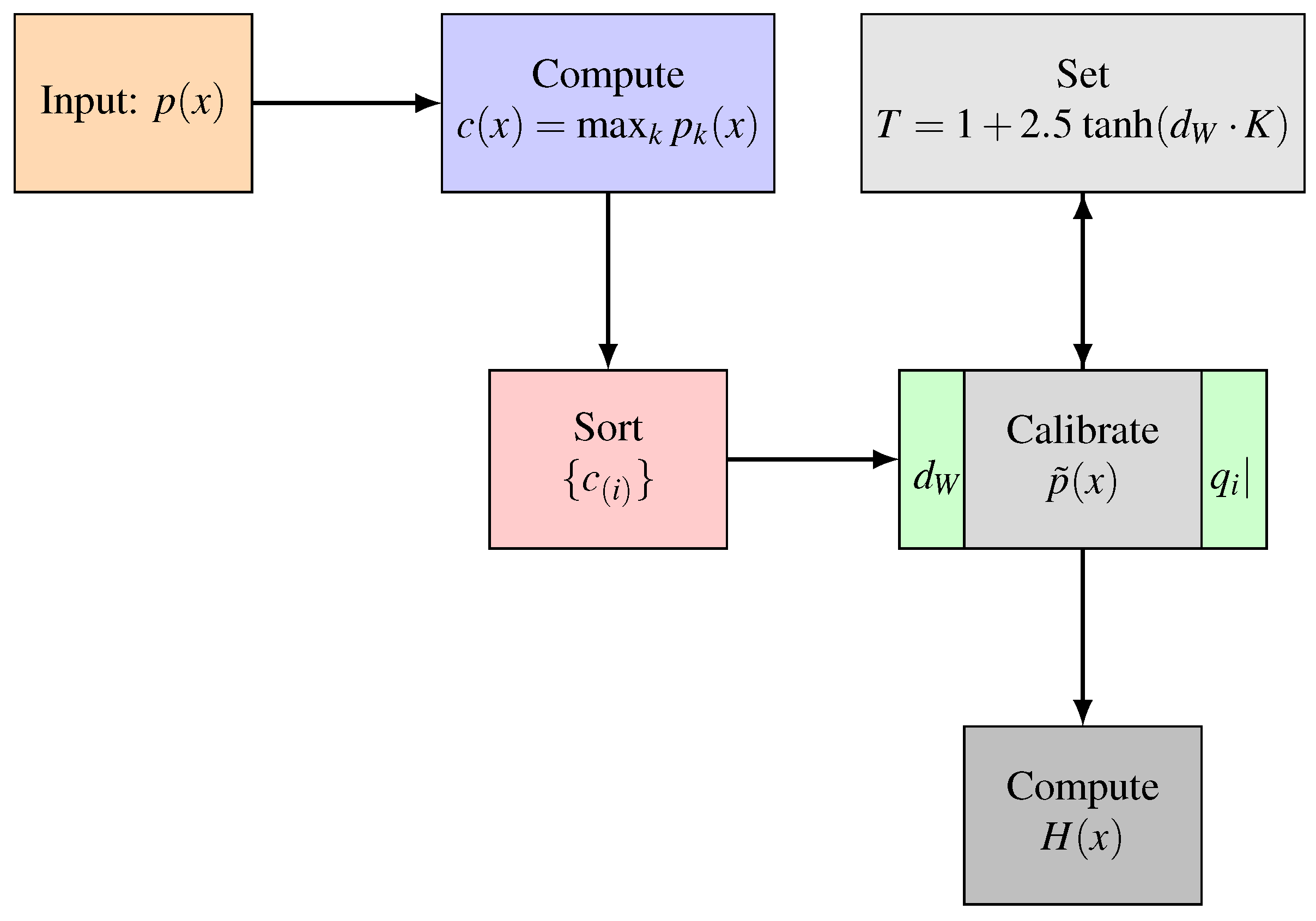
Figure 2.
Workflow of the Diversity-Promoting Sampling component.
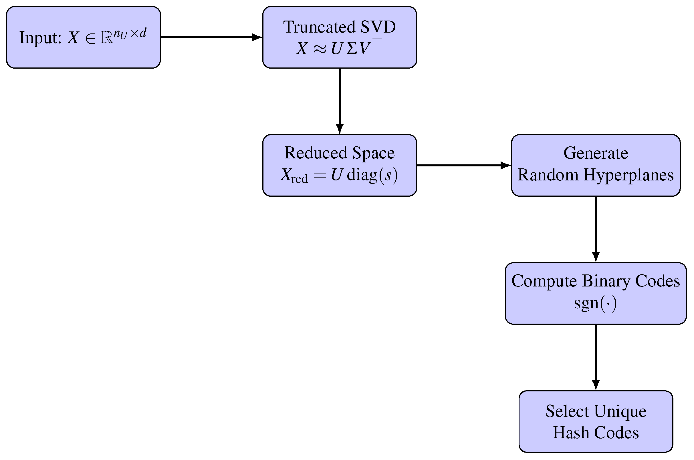
Figure 3.
Workflow of the Dynamic Threshold Optimization Component. This figure illustrates the iterative process: initializing the search range, computing performance metrics and the objective function, performing ternary search iterations, adaptively updating the Lagrangian multipliers, and finally outputting the optimal threshold .
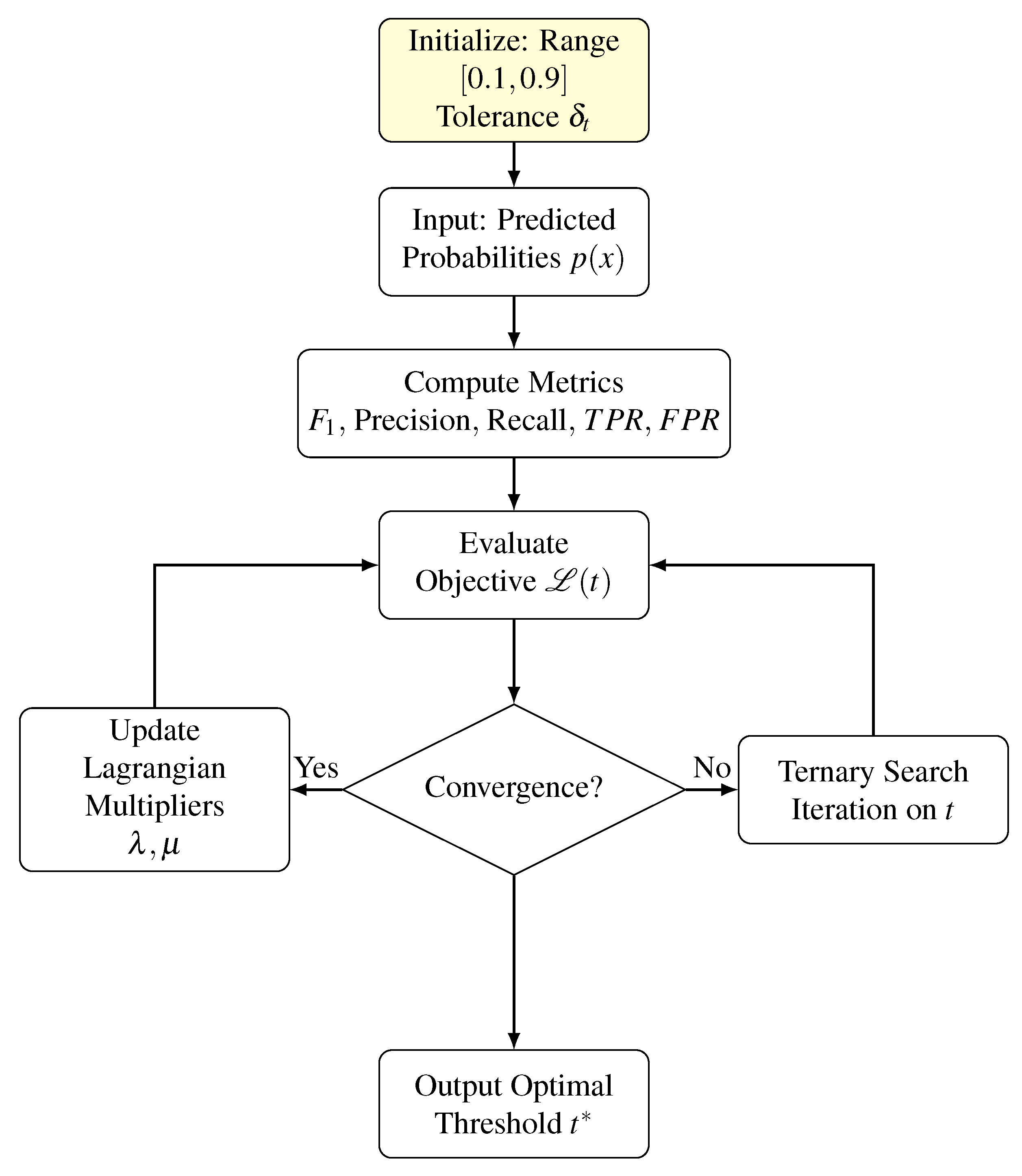
Figure 4.
Overview of the Integrated Iterative Framework.
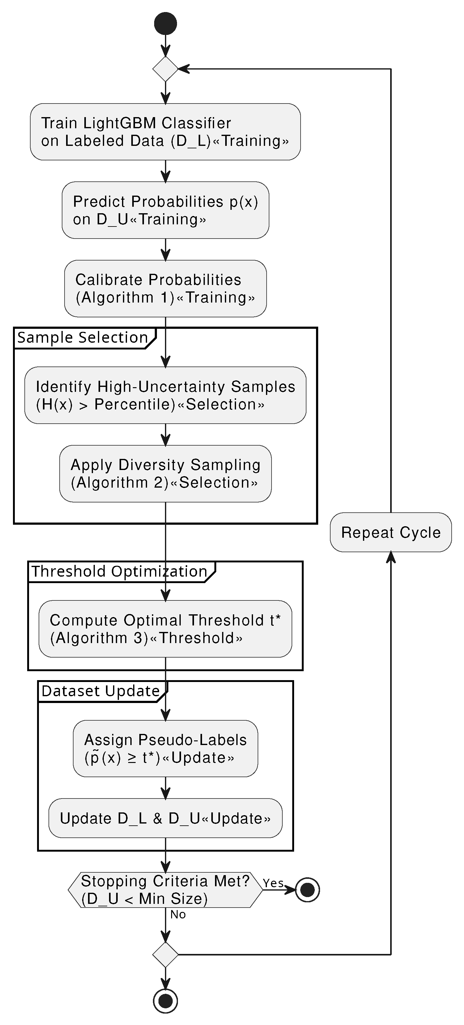
Figure 5.
Bootstrap distribution of AUC scores: Proposed Model vs. Core Set Selection.
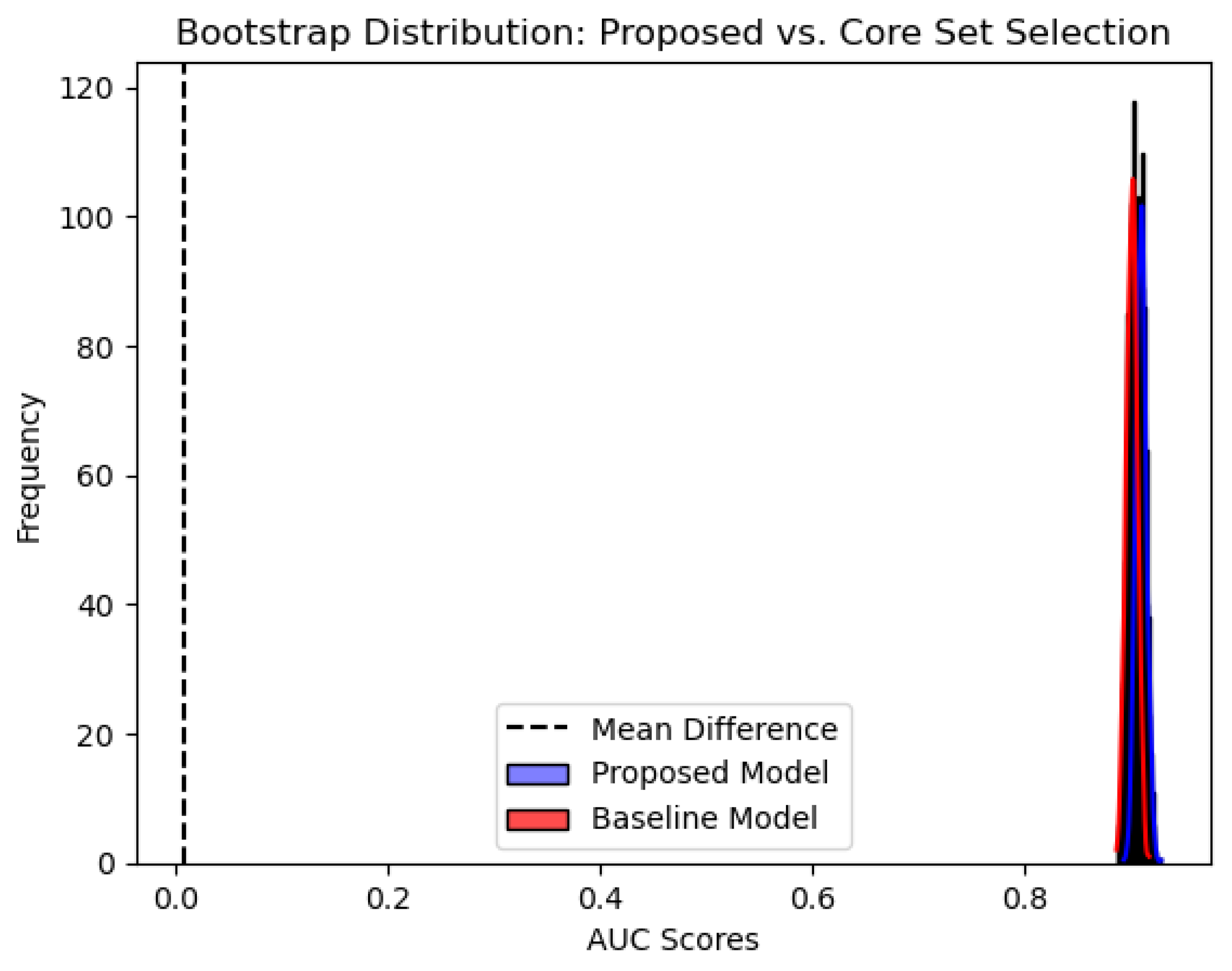
Figure 6.
Bootstrap distribution of AUC scores: Proposed Model vs. Pseudo-Labeling.
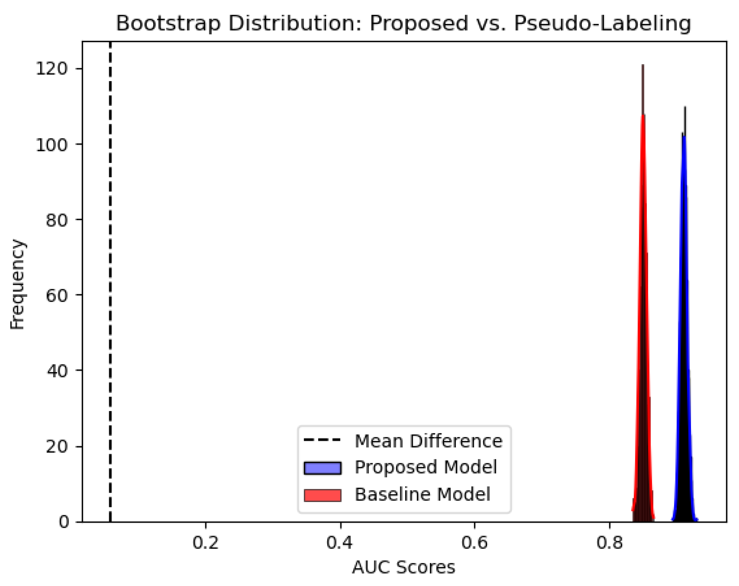
Figure 7.
Distribution of Conditional Entropy for 5% labeled Sparkify dataset. The majority of samples exhibit low entropy, indicating confident pseudo-labeling.
Figure 7.
Distribution of Conditional Entropy for 5% labeled Sparkify dataset. The majority of samples exhibit low entropy, indicating confident pseudo-labeling.
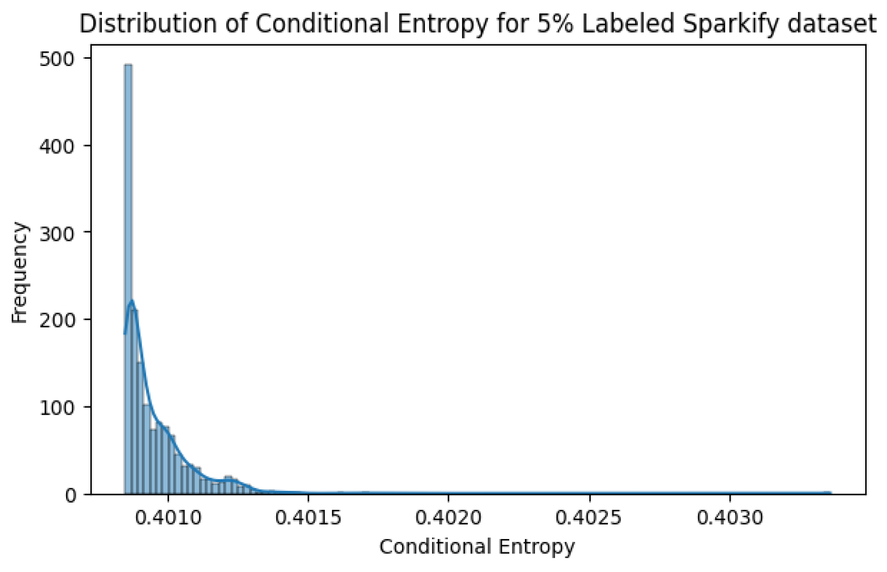
Figure 8.
Distribution of Conditional Entropy for 5% labeled IBM dataset. The majority of samples exhibit low entropy, indicating confident pseudo-labeling.
Figure 8.
Distribution of Conditional Entropy for 5% labeled IBM dataset. The majority of samples exhibit low entropy, indicating confident pseudo-labeling.
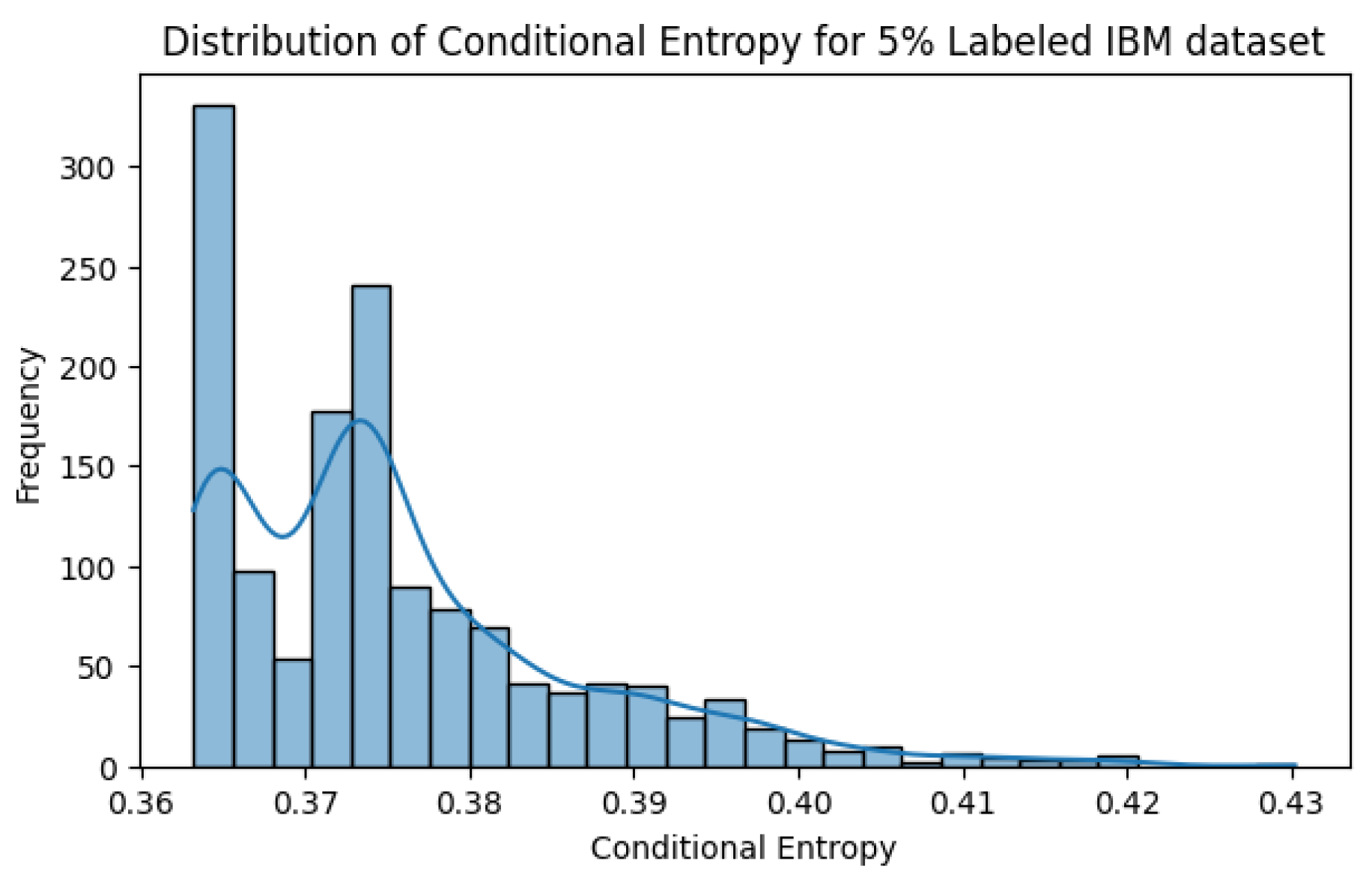
Figure 9.
ROC curve for the Sparkify dataset with 5% labeled data. The proposed model achieves an AUC of 0.91, demonstrating strong predictive performance.
Figure 9.
ROC curve for the Sparkify dataset with 5% labeled data. The proposed model achieves an AUC of 0.91, demonstrating strong predictive performance.
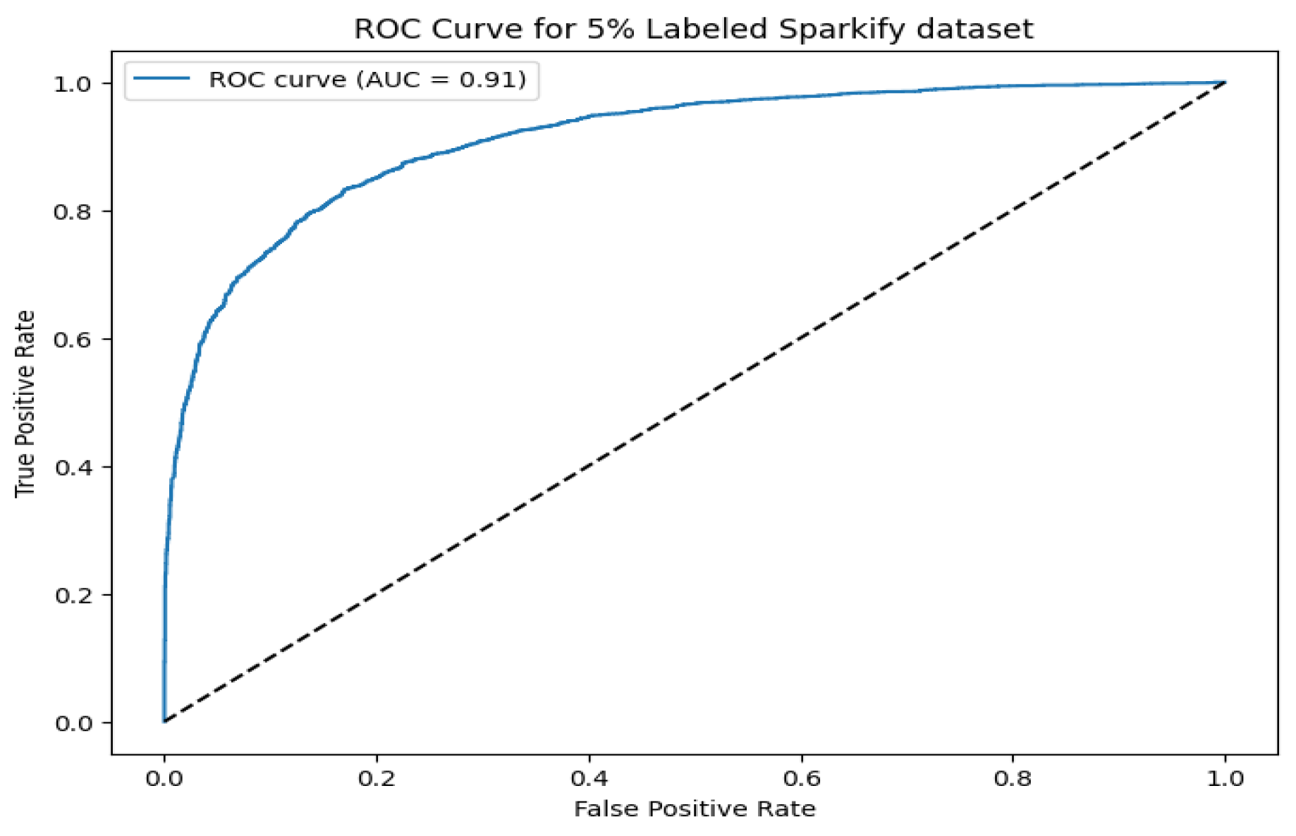
Figure 10.
ROC curve for the IBM dataset with 5% labeled data. The AUC of 0.89 highlights the model’s adaptability across datasets.
Figure 10.
ROC curve for the IBM dataset with 5% labeled data. The AUC of 0.89 highlights the model’s adaptability across datasets.
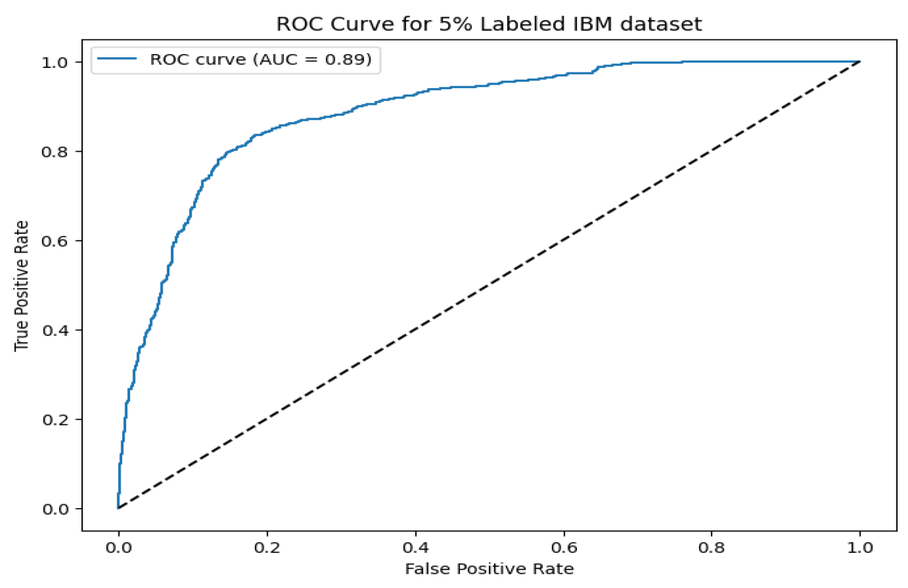

Table 1.
Comparison of Distance Metrics for Calibration
| Metric | Key Strengths | Limitations |
|---|---|---|
| KL Divergence | Sensitive to distribution shape | Asymmetric; unstable with low probabilities |
| TV Distance | Bounded and straightforward | Ignores underlying data geometry |
| Hellinger Distance | Symmetric; robust to small changes | Limited in capturing spatial structure |
| Wasserstein Distance | Integrates magnitude and geometry | Higher computational cost |
Table 2.
Comparison of Calibration Methods
| Method | Adaptivity | Robustness | Complexity |
|---|---|---|---|
| Static Temperature Scaling | No | Low | |
| Platt Scaling | No | Moderate | |
| Isotonic Regression | No | High (data-dependent) | |
| Proposed Adaptive Calibration | Yes | Very High |
Table 3.
Comparison of Diversity Sampling Methods.
| Method | Scalability | Diversity Guarantee | Additional Notes |
|---|---|---|---|
| Random Sampling | Low | No explicit diversity | |
| Clustering-Based Sampling (e.g., k-means) | Moderate | Sensitive to initialization | |
| DPP-based Sampling | High | Computationally prohibitive for large | |
| Proposed Multi-Resolution Hashing | (excl. SVD) | Competitive | Scales well with large datasets |
Table 4.
Comparison of Pseudo-Label Thresholding Methods.
| Method | Adaptivity | Robustness | Search/Optimization | Computational Cost |
|---|---|---|---|---|
| Fixed Threshold | No | Low | N/A | |
| Heuristic Tuning | Partial | Moderate | Manual/Ad hoc | |
| Grid Search | No | Moderate | Exhaustive Search | |
| Bayesian Optimization | Yes | High | Probabilistic Modeling | |
| Proposed Dynamic Optimization (Ternary Search) | Yes | Very High | Ternary Search over |
Table 5.
Dataset Overview and Selection Criteria.
| Dataset | Key Characteristics | Selection Rationale |
|---|---|---|
| Sparkify | Large-scale streaming logs (12.5GB, 26M records, 22K users) | Tests model scalability and temporal behavior modeling |
| IBM Telco | Structured telecom customer data (7,043 customers, 36 features) | Baseline comparison with demographic and service-based features |
| Bank Churn | Banking customer data (10K records, 14 financial features) | Evaluates financial churn prediction and high-cardinality categorical data |
| CrowdAnalytix | High-dimensional service metrics | Assesses feature selection techniques on a large feature space |
Table 6.
Class Distribution Before and After SMOTE.
| Dataset | Original | Balanced | ||
|---|---|---|---|---|
| Non-Churn | Churn | Non-Churn | Churn | |
| Sparkify | 17,274 | 5,003 | 17,274 | 17,274 |
| IBM Telco | 5,174 | 1,869 | 5,174 | 5,174 |
| Bank Churn | 7,963 | 2,037 | 7,963 | 7,963 |
| CrowdAnalytix | 36,336 | 14,711 | 36,336 | 36,336 |
Table 7.
Performance Comparison of Semi-Supervised Models (5% Labeled Data)
| Dataset | Model | AUC | F1 | TPR | FPR |
|---|---|---|---|---|---|
| Sparkify | Proposed Model | 0.9107 | 0.8296 | 0.8643 | 0.2177 |
| Pseudo-Labeling | 0.8501 | 0.8569 | 0.8138 | 0.1001 | |
| Tri-Training | 0.8518 | 0.8576 | 0.8210 | 0.1058 | |
| Label Spreading | 0.7037 | 0.7198 | 0.6676 | 0.2281 | |
| Uncertainty Sampling | 0.9036 | 0.8299 | 0.8068 | 0.1336 | |
| Query-by-Committee | 0.8995 | 0.8194 | 0.7868 | 0.1326 | |
| Diversity Sampling | 0.8946 | 0.8018 | 0.7458 | 0.1136 | |
| Core Set Selection | 0.9022 | 0.8160 | 0.7754 | 0.1243 | |
| BAAL | 0.9106 | 0.8399 | 0.8068 | 0.1136 | |
| Self-Training | 0.8447 | 0.7470 | 0.7127 | 0.1941 | |
| MixMatch | 0.8403 | 0.7330 | 0.6633 | 0.1453 | |
| Mean Teacher | 0.8427 | 0.7470 | 0.6984 | 0.1701 | |
| CoMatch | 0.8174 | 0.7219 | 0.6915 | 0.2226 | |
| IBM Telco | Proposed Model | 0.8902 | 0.8282 | 0.8389 | 0.1899 |
| Pseudo-Labeling | 0.8413 | 0.8294 | 0.8945 | 0.2356 | |
| Tri-Training | 0.8434 | 0.8314 | 0.8984 | 0.2356 | |
| Label Spreading | 0.7909 | 0.7588 | 0.9012 | 0.3836 | |
| Uncertainty Sampling | 0.9333 | 0.8532 | 0.8495 | 0.1937 | |
| Query-by-Committee | 0.9262 | 0.8516 | 0.8696 | 0.1823 | |
| Diversity Sampling | 0.9272 | 0.8543 | 0.8571 | 0.1748 | |
| Core Set Selection | 0.9355 | 0.8632 | 0.8830 | 0.1864 | |
| BAAL | 0.9275 | 0.8595 | 0.8504 | 0.1791 | |
| Self-Training | 0.8664 | 0.8068 | 0.7948 | 0.1876 | |
| MixMatch | 0.8249 | 0.7276 | 0.6836 | 0.2013 | |
| Mean Teacher | 0.6899 | 0.6469 | 0.6472 | 0.3621 | |
| CoMatch | 0.8893 | 0.7896 | 0.7287 | 0.2188 | |
| Banking | Proposed Model | 0.8417 | 0.7630 | 0.7907 | 0.2682 |
| Pseudo-Labeling | 0.7143 | 0.7211 | 0.7147 | 0.2715 | |
| Tri-Training | 0.7150 | 0.7220 | 0.7147 | 0.2707 | |
| Label Spreading | 0.6981 | 0.7025 | 0.7057 | 0.3007 | |
| Query-by-Committee | 0.8600 | 0.7725 | 0.8036 | 0.2671 | |
| Diversity Sampling | 0.8564 | 0.7873 | 0.8281 | 0.2686 | |
| Core Set Selection | 0.8557 | 0.7883 | 0.8152 | 0.2928 | |
| BAAL | 0.8572 | 0.7794 | 0.8088 | 0.2696 | |
| Self-Training | 0.8491 | 0.7756 | 0.8100 | 0.2819 | |
| MixMatch | 0.8416 | 0.7629 | 0.7906 | 0.2731 | |
| Mean Teacher | 0.8415 | 0.7628 | 0.7905 | 0.2793 | |
| CoMatch | 0.7431 | 0.6867 | 0.7366 | 0.3889 | |
| CrowdAnalytix | Proposed Model | 0.7065 | 0.6701 | 0.9781 | 0.9547 |
| Pseudo-Labeling | 0.6119 | 0.6912 | 0.4859 | 0.1035 | |
| Tri-Training | 0.6927 | 0.7254 | 0.6163 | 0.1655 | |
| Label Spreading | 0.5443 | 0.5627 | 0.5191 | 0.3937 | |
| Uncertainty Sampling | 0.7214 | 0.6447 | 0.5975 | 0.2597 | |
| Query-by-Committee | 0.7142 | 0.6378 | 0.5927 | 0.2695 | |
| Diversity Sampling | 0.7137 | 0.6355 | 0.5881 | 0.2664 | |
| Core Set Selection | 0.7160 | 0.6373 | 0.5945 | 0.2749 | |
| BAAL | 0.7214 | 0.6447 | 0.5975 | 0.2597 | |
| Self-Training | 0.6853 | 0.6111 | 0.5699 | 0.2995 | |
| MixMatch | 0.5763 | 0.5704 | 0.5848 | 0.4724 | |
| Mean Teacher | 0.5722 | 0.5382 | 0.5156 | 0.4063 | |
| CoMatch | 0.5769 | 0.5615 | 0.5707 | 0.4688 |
Table 8.
Performance Comparison of Semi-Supervised Models (10% Labeled Data).
| Dataset | Model | AUC | F1 | TPR | FPR |
|---|---|---|---|---|---|
| Sparkify | Proposed Model | 0.9326 | 0.8650 | 0.8472 | 0.1107 |
| Pseudo-Labeling | 0.8633 | 0.8697 | 0.8245 | 0.0851 | |
| Tri-Training | 0.8634 | 0.8676 | 0.8393 | 0.1041 | |
| Label Spreading | 0.7371 | 0.7456 | 0.7156 | 0.2243 | |
| Uncertainty Sampling | 0.9236 | 0.8487 | 0.8178 | 0.1087 | |
| Query-by-Committee | 0.9180 | 0.8372 | 0.8065 | 0.1194 | |
| Diversity Sampling | 0.9179 | 0.8349 | 0.7960 | 0.1101 | |
| Core Set Selection | 0.9188 | 0.8390 | 0.8094 | 0.1191 | |
| BAAL | 0.9236 | 0.8487 | 0.8178 | 0.1087 | |
| Self-Training | 0.8833 | 0.7825 | 0.7467 | 0.1606 | |
| MixMatch | 0.8526 | 0.7631 | 0.7382 | 0.1952 | |
| Mean Teacher | 0.8514 | 0.7687 | 0.7801 | 0.2477 | |
| CoMatch | 0.8071 | 0.7284 | 0.7281 | 0.2690 | |
| IBM Telco | Proposed Model | 0.9232 | 0.8445 | 0.8667 | 0.1889 |
| Pseudo-Labeling | 0.8445 | 0.8349 | 0.8366 | 0.2181 | |
| Tri-Training | 0.8441 | 0.8359 | 0.8210 | 0.2084 | |
| Label Spreading | 0.8046 | 0.7843 | 0.8600 | 0.3096 | |
| Uncertainty Sampling | 0.9384 | 0.8401 | 0.8582 | 0.1890 | |
| Query-by-Committee | 0.9381 | 0.8344 | 0.8155 | 0.1801 | |
| Diversity Sampling | 0.9335 | 0.8378 | 0.8541 | 0.1990 | |
| Core Set Selection | 0.9364 | 0.8320 | 0.8619 | 0.1894 | |
| BAAL | 0.9396 | 0.8299 | 0.8793 | 0.2098 | |
| Self-Training | 0.9266 | 0.8629 | 0.8593 | 0.2195 | |
| MixMatch | 0.9255 | 0.8427 | 0.8217 | 0.1996 | |
| Mean Teacher | 0.9328 | 0.8444 | 0.8266 | 0.2217 | |
| CoMatch | 0.8946 | 0.8054 | 0.7661 | 0.1383 | |
| Banking | Proposed Model | 0.8998 | 0.8185 | 0.8332 | 0.1929 |
| Pseudo-Labeling | 0.7793 | 0.7846 | 0.7798 | 0.2107 | |
| Tri-Training | 0.7790 | 0.7845 | 0.7785 | 0.2094 | |
| Label Spreading | 0.7626 | 0.7674 | 0.7663 | 0.2315 | |
| Uncertainty Sampling | 0.8572 | 0.7794 | 0.8088 | 0.2535 | |
| Query-by-Committee | 0.8600 | 0.7725 | 0.8036 | 0.2633 | |
| Diversity Sampling | 0.8564 | 0.7873 | 0.8281 | 0.2621 | |
| Core Set Selection | 0.8557 | 0.7883 | 0.8152 | 0.2407 | |
| BAAL | 0.8572 | 0.7794 | 0.8088 | 0.2535 | |
| Self-Training | 0.8491 | 0.7756 | 0.8100 | 0.2652 | |
| MixMatch | 0.8925 | 0.8072 | 0.8545 | 0.2498 | |
| Mean Teacher | 0.8864 | 0.8010 | 0.8487 | 0.2572 | |
| CoMatch | 0.7361 | 0.6823 | 0.7592 | 0.4434 | |
| CrowdAnalytix | Proposed Model | 0.7948 | 0.7137 | 0.5801 | 0.0463 |
| Pseudo-Labeling | 0.5283 | 0.6570 | 0.3835 | 0.0690 | |
| Tri-Training | 0.6811 | 0.7324 | 0.5700 | 0.1052 | |
| Label Spreading | 0.5637 | 0.5773 | 0.5426 | 0.3880 | |
| Uncertainty Sampling | 0.7348 | 0.6591 | 0.6117 | 0.2481 | |
| Query-by-Committee | 0.7307 | 0.6546 | 0.6099 | 0.2571 | |
| Diversity Sampling | 0.7261 | 0.6488 | 0.6019 | 0.2569 | |
| Core Set Selection | 0.7322 | 0.6578 | 0.6180 | 0.2646 | |
| BAAL | 0.7348 | 0.6591 | 0.6117 | 0.2481 | |
| Self-Training | 0.7117 | 0.6170 | 0.5437 | 0.2216 | |
| MixMatch | 0.5955 | 0.5509 | 0.5215 | 0.3771 | |
| Mean Teacher | 0.6022 | 0.5720 | 0.5621 | 0.4090 | |
| CoMatch | 0.5772 | 0.5409 | 0.5258 | 0.4241 |
Table 9.
Proposed Model Execution Time (in seconds).
| Dataset | 5% Labeled Data | 10% Labeled Data |
|---|---|---|
| Sparkify Churn Dataset | 89.39 | 82.67 |
| IBM Telecom Churn Dataset | 78.24 | 19.73 |
| Bank Churn Dataset | 11.84 | 27.17 |
| CrowdAnalytix Telecom Churn Dataset | 220.41 | 79.30 |
Table 10.
Ablation Study Results (5% Labeled Data)
| Variant | Final AUC | Final F1 | Final TPR | Final FPR | Execution Time (s) |
|---|---|---|---|---|---|
| Proposed Model | 0.9107 | 0.8296 | 0.8643 | 0.2177 | 89.39 |
| No WCE | 0.5322 | 0.6650 | 1.0000 | 0.4981 | 128.41 |
| No LTO | 0.5339 | 0.5517 | 0.5997 | 0.5108 | 101.97 |
| No Diversity | 0.5522 | 0.6649 | 0.9997 | 0.4981 | 123.43 |
Table 11.
Ablation Study Results (10% Labeled Data)
| Variant | Final AUC | Final F1 | Final TPR | Final FPR | Execution Time (s) |
|---|---|---|---|---|---|
| Proposed Model | 0.9326 | 0.8650 | 0.8472 | 0.1107 | 82.67 |
| No WCE | 0.4632 | 0.6646 | 0.9988 | 0.4980 | 82.45 |
| No LTO | 0.5007 | 0.4719 | 0.4372 | 0.5124 | 70.34 |
| No Diversity | 0.4711 | 0.6643 | 0.9983 | 0.4978 | 80.24 |
Table 12.
Summary of Statistical Test Results. The Wilcoxon signed-rank test statistic and p-values are provided along with the bootstrapped mean AUC difference and Cohen’s d effect size.
Table 12.
Summary of Statistical Test Results. The Wilcoxon signed-rank test statistic and p-values are provided along with the bootstrapped mean AUC difference and Cohen’s d effect size.
| Comparison | Wilcoxon Signed-Rank | Bootstrapped AUC Difference | Cohen’s d |
|---|---|---|---|
| Proposed vs. Pseudo-Labeling | (0.0000, 0.0000) | 0.0604 [0.0599, 0.0608] | 12.2104 |
| Proposed vs. BAAL | (245398.0000, 0.5953) | 0.0002 [-0.0002, 0.0006] | 0.0341 |
| Proposed vs. Core Set | (20555.0000, 0.0000) | 0.0087 [0.0083, 0.0091] | 1.7321 |
| Proposed vs. CoMatch | (0.0000, 0.0000) | 0.0937 [0.0932, 0.0941] | 18.9980 |
Disclaimer/Publisher’s Note: The statements, opinions and data contained in all publications are solely those of the individual author(s) and contributor(s) and not of MDPI and/or the editor(s). MDPI and/or the editor(s) disclaim responsibility for any injury to people or property resulting from any ideas, methods, instructions or products referred to in the content. |
© 2025 by the authors. Licensee MDPI, Basel, Switzerland. This article is an open access article distributed under the terms and conditions of the Creative Commons Attribution (CC BY) license (http://creativecommons.org/licenses/by/4.0/).
Copyright: This open access article is published under a Creative Commons CC BY 4.0 license, which permit the free download, distribution, and reuse, provided that the author and preprint are cited in any reuse.


