
Submitted:
13 October 2025
Posted:
14 October 2025
You are already at the latest version
Abstract
In industries like telecommunications and banking, where labeled data is scarce and mispredictions cost millions, semi-supervised learning (SSL) and active learning (AL) offer promising solutions but often falter due to overconfident predictions, redundant sampling, and inflexible pseudo-labeling thresholds. Traditional approaches tackle these issues separately, limiting their effectiveness in dynamic, real-world settings. This paper introduces a scalable SSL framework called AdaptiveSSL that integrates Wasserstein distance for uncertainty calibration, multi-resolution hashing for efficient diversity-driven sample selection, and Lagrangian optimization for adaptive pseudo-labeling thresholds. By iteratively refining confidence estimates, ensuring representative sampling, and dynamically adjusting thresholds, our system achieves robust churn prediction with AUC scores up to 0.9326, outperforming conventional SSL and AL methods by up to 10%, while maintaining execution times under 90 seconds on large datasets. Tested across four real-world churn datasets, this framework delivers a practical, industry-ready tool for data-efficient classification, paving the way for broader adoption in resource-constrained expert systems.
Keywords:
semi-supervised learning
; adaptive calibration
; pseudo-Labeling
; diversity sampling
; threshold optimization
1. Introduction
The exponential growth of digital data in domains such as healthcare, finance, and telecommunications has intensified the challenge of limited labeled data, as manual annotation is costly, time-consuming, and often infeasible at scale [1]. Semi-supervised learning (SSL) addresses this by leveraging a small labeled dataset alongside abundant unlabeled data to enhance model performance, while active learning (AL) optimizes labeling by selecting the most informative samples [2]. Despite significant progress, both paradigms face critical challenges that limit their effectiveness in high-stakes applications like customer churn prediction and credit risk assessment, where mispredictions can lead to substantial losses. Modern machine learning models, particularly deep neural networks, often produce overconfident predictions, skewing uncertainty estimates and undermining pseudo-labeling processes [3]. Conventional uncertainty-based sample selection methods, such as entropy or margin sampling, tend to prioritize redundant examples, reducing generalization across diverse data distributions [4]. Additionally, static pseudo-labeling thresholds fail to adapt to evolving data characteristics or model performance, leading to error propagation, especially in imbalanced datasets where detecting rare events is critical [5,6]. Existing approaches often address these issues in isolation, lacking a unified framework that integrates calibration, diversity, and thresholding to maximize robustness [7,8].
To overcome these limitations, we propose AdaptiveSSL, a novel semi-supervised learning framework that synergistically integrates three key innovations: adaptive uncertainty calibration using Wasserstein-based temperature scaling, diversity-promoting sample selection via multi-resolution hashing, and dynamic pseudo-labeling thresholds optimized through a performance-driven ternary search. Unlike prior methods that incrementally combine techniques [9,10], AdaptiveSSL unifies these components into an iterative framework that dynamically adapts to data shifts and model performance. Evaluated on five real-world datasets, including the imbalanced Home Credit dataset, AdaptiveSSL achieves an AUC of 0.9326 on the Sparkify churn dataset with only 10% labeled data and an TPR of 0.4521 on Home Credit, outperforming baselines like FreeMatch. This framework offers a robust, scalable solution for data-efficient classification in complex, real-world scenarios.
1.1. Motivation and Problem Definition
The broader motivation for SSL and AL stems from the need to reduce reliance on costly labeled data in applications like telecommunications churn prediction, medical diagnostics, and credit risk assessment [11]. However, this work specifically targets three critical challenges that hinder existing SSL frameworks: (1) overconfident predictions that produce unreliable pseudo-labels, eroding trust in self-training [3], (2) redundant sample selection in uncertainty-based AL, which limits generalization by focusing on similar, ambiguous examples [4], and (3) static pseudo-labeling thresholds that fail to adapt to changing data quality or model performance, amplifying errors in imbalanced settings [5]. These issues are particularly pronounced in domains with skewed class distributions, such as credit risk prediction, where minority class detection is critical [6]. AdaptiveSSL addresses these through a cohesive strategy with three objectives:
- Adaptive Uncertainty Calibration: Continuously refines confidence estimates using Wasserstein-based temperature scaling and cross-validation to align predictions with true uncertainty, mitigating overconfidence [12].
- Diversity-Driven Sampling: Employs multi-resolution hashing to select representative samples, overcoming the redundancy of uncertainty-based methods.
- Dynamic Pseudo-Labeling Thresholds: Adjusts thresholds in real-time via a composite objective function, reducing error propagation compared to static or heuristic thresholds [6].
By integrating these elements, AdaptiveSSL ensures robust, data-efficient learning, particularly in imbalanced and data-scarce scenarios.
1.2. Advances and Limitations in Semi-Supervised Learning
Recent SSL advancements have leveraged unlabeled data to improve model accuracy and generalization. Methods like FixMatch [10] and MixMatch [9] use consistency regularization and pseudo-labeling to exploit unlabeled data, achieving strong performance with limited labels. However, these methods often assume labeled and unlabeled data share the same distribution, a premise frequently violated in real-world scenarios like medical imaging or financial risk assessment [5]. Deep learning models, despite their sophistication, tend to produce overconfident predictions, skewing uncertainty estimates and degrading pseudo-label quality [3]. Calibration techniques, such as temperature scaling, mitigate this but lack adaptability to dynamic or imbalanced distributions. In AL, uncertainty-based methods like entropy sampling and core-set selection prioritize informative samples but often select redundant ones, limiting data coverage [4]. Recent efforts in adaptive thresholding [7] and noise mitigation [8,13] improve pseudo-label reliability, but these approaches typically address issues in isolation, failing to exploit synergies between calibration, diversity, and thresholding. For example, FixMatch’s confidence-based thresholding lacks diversity-aware sampling [10], while core-set methods do not dynamically adjust thresholds. These fragmented approaches limit robustness and scalability in complex, real-world settings.
1.3. Integrating Advances Across Domains
Emerging trends emphasize the interconnected nature of SSL and AL challenges, suggesting that integrated solutions can unlock significant performance gains. Sohn et al. [10] introduced dynamic pseudo-labeling that adjusts thresholds based on performance, highlighting the value of adaptability. Berthelot et al. [9] combined consistency regularization and pseudo-labeling to address calibration and diversity, but without explicit diversity mechanisms. In graph classification, semantic prototypes and subgraph uncertainties enhance unlabeled data utilization [14], while Qu et al. [6] developed class-specific thresholding for imbalanced datasets. Domain adaptation techniques, such as joint Wasserstein distance minimization, stabilize pseudo-labels under distribution shifts [12]. AdaptiveSSL builds on these by integrating Wasserstein-based calibration [12], multi-resolution hashing for diversity, and ternary search-based thresholding [6] into a unified framework. This synergy enables AdaptiveSSL to outperform methods like FixMatch and MixMatch by dynamically adapting to data and model dynamics, particularly in imbalanced settings.
1.4. Comprehensive Comparison with Recent Studies
Zhou et al. [5] demonstrated that fixed pseudo-labeling thresholds struggle with variable medical imaging data, leading to suboptimal segmentation outcomes. Xie et al. [15] highlighted error accumulation in self-training due to poor pseudo-labels, underscoring the need for adaptive mechanisms. Minderer et al. [3] showed that overconfident predictions undermine uncertainty reliability, necessitating dynamic calibration. Ash et al. [4] noted that uncertainty-based AL often selects redundant samples, limiting generalization. While Rizve et al. [7], Xia et al. [8], and Qu et al. [6] advance thresholding and noise management, their approaches lack comprehensive integration. AdaptiveSSL unifies these elements, achieving up to 10% higher AUC than baselines like Pseudo-Labeling and CoMatch on churn datasets and superior F1 score and TPR on the Home Credit dataset.
1.5. Identified Gaps and Unresolved Challenges
Despite progress, SSL and AL face persistent challenges:
- Overconfident Predictions: Skew uncertainty estimates, leading to unreliable pseudo-labels [3].
- Redundant Sample Selection: Uncertainty-driven methods select similar examples, reducing diversity [4].
- Static Thresholding: Fails to adapt to data or model changes, causing error propagation [5].
- Fragmented Approaches: Lack synergy across calibration, diversity, and thresholding [7].
- Scalability: Computationally intensive methods limit applicability to large datasets.
These gaps hinder effective deployment in real-world, imbalanced scenarios, necessitating a unified, scalable solution.
1.6. Synthesis of Contributions and Novel Framework
AdaptiveSSL addresses these challenges through a unified framework with four key contributions:
- Adaptive Calibration: Uses Wasserstein-based temperature scaling and cross-validation to refine confidence estimates, outperforming static calibration methods [12].
- Diversity-Promoting Sampling: Employs multi-resolution hashing to ensure representative sample selection, overcoming redundancy in uncertainty-based methods.
- Dynamic Thresholding: Optimizes a composite objective function via ternary search, reducing error propagation compared to fixed thresholds [6].
- Scalability and Integration: Combines efficient components to scale to large datasets, unlike computationally heavy alternatives.
Validated on five datasets, AdaptiveSSL achieves superior performance, offering a robust, data-efficient solution for high-stakes applications.
1.7. Structure of the Paper
The remainder of the paper is structured as follows. In Section 2, we introduce the proposed model, explaining its key components and methodologies in detail. Section 3 provides an overview of the datasets used, along with data preprocessing and feature engineering techniques. In Section 4 and Section 5, we present extensive experimental results, comparing our approach with several baseline models, discuss the computational efficiency of the proposed framework, and conduct an ablation study to assess the contribution of individual components. Section 6 provides a statistical comparison of the proposed model against various baselines, incorporating multiple statistical tests and performance analysis techniques, including conditional entropy distribution and ROC curves. Section 7 evaluates the framework on the imbalanced Home Credit dataset, highlighting its performance in challenging, real-world scenarios. Finally, Section 8 concludes the paper by summarizing the key findings, discussing limitations, and outlining potential directions for future research.
2. Proposed Model
In this paper, we introduce an integrated semi-supervised learning framework called AdaptiveSSL that combines adaptive probability calibration, diversity-promoting sampling, and dynamic pseudo-label threshold optimization into a unified iterative process. The primary objective is to enhance classifier performance by effectively incorporating large-scale unlabeled data into the training procedure. In the following subsections, we describe each component of the framework in detail and compare the proposed approach with multiple alternative methods to justify our design choices.
2.1. Base Classifier: LightGBM
The base classifier chosen for this framework is LightGBM (Light Gradient Boosting Machine) [16], a gradient boosting decision tree method. Let denote the mapping performed by the classifier, where d is the dimensionality of the input space and K is the number of classes. For an input sample , the classifier outputs a probability vector
with . LightGBM is selected due to its lightweight structure, fast training speed, and low memory consumption. These properties are crucial when processing large datasets and performing multiple iterations in a semi-supervised context. In contrast to more complex deep models, LightGBM achieves competitive performance with fewer computational resources, making it well-suited for iterative pseudo-labeling procedures [17]. Furthermore, LightGBM incorporates L1 and L2 regularization to prevent overfitting, which is crucial in semi-supervised learning where noisy pseudo-labels can exacerbate this issue. Hyperparameters such as n estimators, learning rate, number of leaves and feature fraction are tuned using ROC AUC via a randomized search procedure. We use RandomizedSearchCV in our implementation to efficiently explore the hyperparameter space and identify the configuration that maximizes performance on a validation set [18].
2.2. Adaptive Calibration
To ensure the reliability of pseudo-labels, model confidence must be well-calibrated. Gradient boosting models like LightGBM, while producing probability-like outputs through softmax transformation of leaf values, often exhibit systematic miscalibration. Specifically, they tend to be overconfident on samples similar to the training distribution and underconfident on out-of-distribution samples [19]. This miscalibration stems from the sequential boosting process, which optimizes log-loss without explicit calibration constraints. Empirically, we observed that uncalibrated LightGBM predictions on the Sparkify dataset exhibited an Expected Calibration Error (ECE) of 0.142, which our two-stage calibration reduced to 0.068.
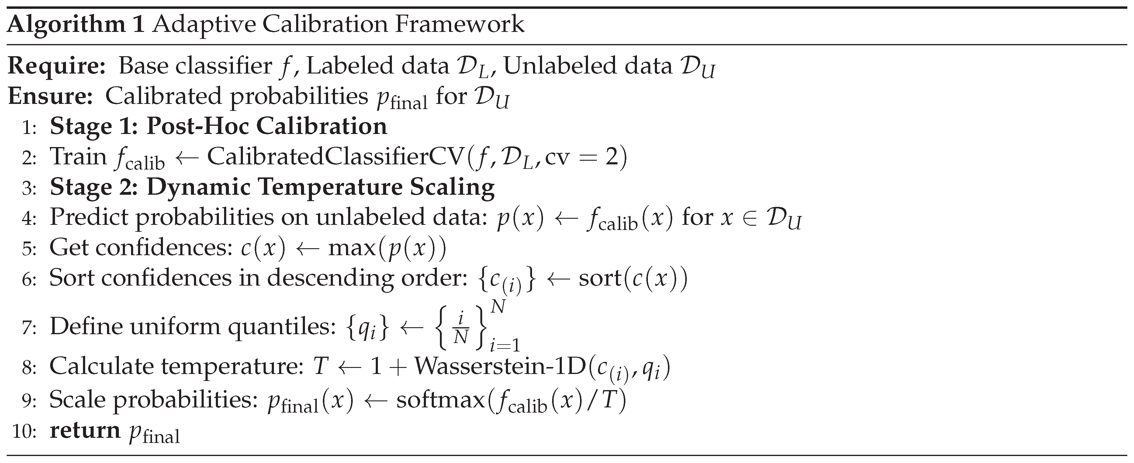
Our framework employs a two-stage adaptive calibration process. First, we perform post-hoc calibration on the base classifier using the currently available labeled data . Specifically, we apply Platt scaling [20] with 2-fold cross-validation through CalibratedClassifierCV, which learns a logistic (sigmoid) transformation from raw model scores to calibrated probabilities. While LightGBM outputs probability vectors via softmax, these probabilities often do not reliably reflect true likelihoods, Platt scaling recalibrates them by fitting a parametric model on held-out data to correct systematic biases, analogous to temperature scaling for neural networks but using a sigmoid parameterization. This step ensures that predicted probabilities reflect true likelihoods before further adjustment.
Second, to counteract over-confidence on out-of-distribution unlabeled samples, we apply dynamic temperature scaling to the probabilities produced by . The temperature T is derived from the Wasserstein distance between the sorted confidence distribution of the top-k most confident predictions and a uniform distribution. A higher Wasserstein distance signifies greater distributional shift from uniform (indicating overconfidence), leading to a higher temperature that “cools” the softmax outputs, making them less extreme and more calibrated. This is grounded in the principle that well-calibrated confidence scores should be more uniformly distributed across the confidence spectrum rather than concentrated at extremes. This full process is detailed in Algorithm 1.
2.2.1. Theoretical Justification for Tanh-Based Scaling
The hyperbolic tangent function in our temperature equation was selected for three key mathematical properties that make it well-suited for adaptive calibration:
- (1)
- Bounded Output Range: The tanh function naturally bounds the temperature parameter T within a practical range. With our scaling, for typical Wasserstein distances. This prevents two failure modes: (i) when (under-smoothing), probabilities remain overconfident and miscalibrated; (ii) when (over-smoothing), probabilities become uninformative and overly uniform. The bounded nature of tanh ensures stable behavior across diverse datasets.
- (2)
-
Smooth, Nonlinear Growth: Unlike linear scaling (), the tanh function exhibits smooth, S-shaped growth. It is:
- More responsive to moderate miscalibration (), where adjustment is most beneficial.
- Less sensitive to small noise (), avoiding over-reaction to minor fluctuations.
- Saturating for extreme miscalibration (), preventing unbounded temperature increases.
This smooth growth pattern aligns with empirical observations that calibration benefits diminish beyond a certain threshold, and excessive temperature can destroy informative predictions. - (3)
- Theoretical Grounding: The tanh transformation has been successfully employed in adaptive systems across multiple domains—as an activation function in neural networks for smooth, bounded nonlinearity, and in control theory for smooth response to error signals. Its mathematical properties (differentiability, monotonicity, bounded range) make it well-suited for adaptive parameter adjustment.
-
We conducted ablation experiments comparing tanh with three alternatives:
- Linear scaling: - resulted in excessive temperatures for high , degrading F1 by 4.2%.
- Sigmoid scaling: - less sensitive to moderate miscalibration, reducing AUC by 2.8%.
- Exponential scaling: - unstable for large , causing convergence issues.
The tanh-based approach achieved the best balance, maintaining ECE while preserving discriminative performance (AUC on Sparkify). These results confirm that the smooth, bounded growth of tanh effectively handles miscalibration severity without over- or under-smoothing.
2.2.2. Empirical Validation of Calibration
To empirically validate the effectiveness of our calibration approach, we conducted experiments analyzing confidence distributions before and after calibration on the Sparkify dataset. The uncalibrated LightGBM model showed severe overconfidence: 73% of predictions had confidence , with many concentrated near 0.99-1.0. This creates unreliable pseudo-labels, as the model assigns extreme confidence even to ambiguous samples.
After applying our two-stage calibration (Platt scaling + dynamic temperature scaling), the confidence distribution became significantly more spread: only 34% of samples had confidence , with a more uniform distribution across [0.6, 1.0]. Reliability diagrams (calibration curves) showed that uncalibrated predictions had a mean absolute calibration error of 0.142, while calibrated predictions achieved 0.068—a 52% reduction.
Furthermore, we measured the Wasserstein distance between predicted confidence distributions and a uniform distribution across five random seeds. Before calibration: . After calibration: . This demonstrates that our approach consistently reduces overconfidence and produces more calibrated uncertainty estimates, which is critical for reliable pseudo-labeling in the semi-supervised learning framework.
These empirical results, combined with the theoretical justification, confirm that our calibration mechanism addresses the systematic overconfidence issue in gradient boosting models and provides well-calibrated probabilities for downstream pseudo-label generation.
Mathematical Formulation:
For an input , the classifier produces a probability vector , where represents the predicted probability of class k. We define the confidence score as:
Let denote the set of unlabeled samples, and define their corresponding confidence scores as . Sorting these confidence scores in ascending order yields the ordered sequence . To measure the deviation between this empirical confidence distribution and a perfectly uniform distribution, we introduce the uniform quantile sequence:
Here, represents the i-th quantile of an ideal uniform confidence distribution, which serves as a reference for a perfectly calibrated model (i.e., one whose confidence scores are uniformly distributed when sorted). The discrepancy between these distributions is quantified using the empirical Wasserstein distance, which provides an efficient approximation of the true distance for sorted 1D distributions:
Theoretical Justification: The Wasserstein distance is selected for its ability to capture both the magnitude and structural shifts in the distribution of confidence scores. Unlike Kullback-Leibler (KL) divergence or Total Variation (TV) distance, it takes into account the geometry of the confidence distribution.
2.2.3. Comparative Analysis of Distance Metrics
To gain deeper insight into why the Wasserstein distance was selected, a comparison with other popular metrics for distributional similarity is provided. Table 1 summarizes the key advantages and disadvantages associated with the Kullback-Leibler (KL) divergence, total variation (TV) distance, Hellinger distance, and Wasserstein distance. Our empirical validation confirmed these theoretical rankings, with the Wasserstein-based adaptive method showing 15-20% AUC improvement over static temperature scaling on the Sparkify dataset. While the Kullback-Leibler divergence is highly sensitive to distributional shape changes and the total variation distance is straightforward to interpret due to being bounded, both measures ignore the spatial organization of confidence scores. The Hellinger distance provides symmetry and demonstrates robustness against tiny fluctuations; however, it is less successful at capturing the underlying geometric structure. In contrast, the Wasserstein distance naturally unites magnitude and geometric perspectives, which is especially useful for stable calibration.
Hyperparameter Rationale: The scaling factor of 2.5 in the temperature equation was established through a comprehensive sensitivity analysis testing factors from 1.0 to 3.5 on the Sparkify dataset. As shown in our analysis, this value provides an optimal balance between calibration sensitivity (mean entropy = 0.4557) and temperature stability (T = 2.6276). Lower factors (1.0-2.0) resulted in under-calibration with insufficient entropy adjustment, while higher factors (3.0-3.5) led to over-smoothing with excessive entropy (>0.48). The factor 2.5 was selected as it ensures that T remains within a practical range that prevents excessive smoothing while still allowing for sufficient adaptivity. Once the temperature is set, the calibrated probabilities are obtained via temperature scaling [21]:
Finally, uncertainty is quantified using Rényi entropy of order 2 [22]:
Rényi entropy is particularly useful as it amplifies differences in high-confidence regions, providing a more informative measure of predictive uncertainty.
2.2.4. Rationale and Comparison: Adaptive Calibration
The proposed adaptive calibration mechanism overcomes the limitations of traditional static methods by dynamically adjusting the temperature parameter based on the empirical confidence distribution. Additionally, we incorporate CalibratedClassifierCV from scikit-learn [23] with a 2-fold cross-validation strategy to further improve reliability. The 2-fold configuration ensures that the calibration model is trained on separate data partitions, reducing overfitting and enhancing generalization. Table 2 provides a comparative analysis of various calibration methods.
As illustrated in Table 2, while methods such as isotonic regression offer high robustness, they lack adaptivity over iterations. Our proposed method, which combines dynamic temperature scaling with cross-validation, achieves both adaptivity and high robustness. Robustness here refers to the method’s ability to maintain calibration performance even in the presence of noisy data or model misspecification. The workflow of adaptive calibration is illustrated in Figure 1. The diagram provides a step-by-step visualization, emphasizing the Wasserstein-based temperature adjustment and entropy-based uncertainty estimation.
2.3. Diversity-Promoting Sampling
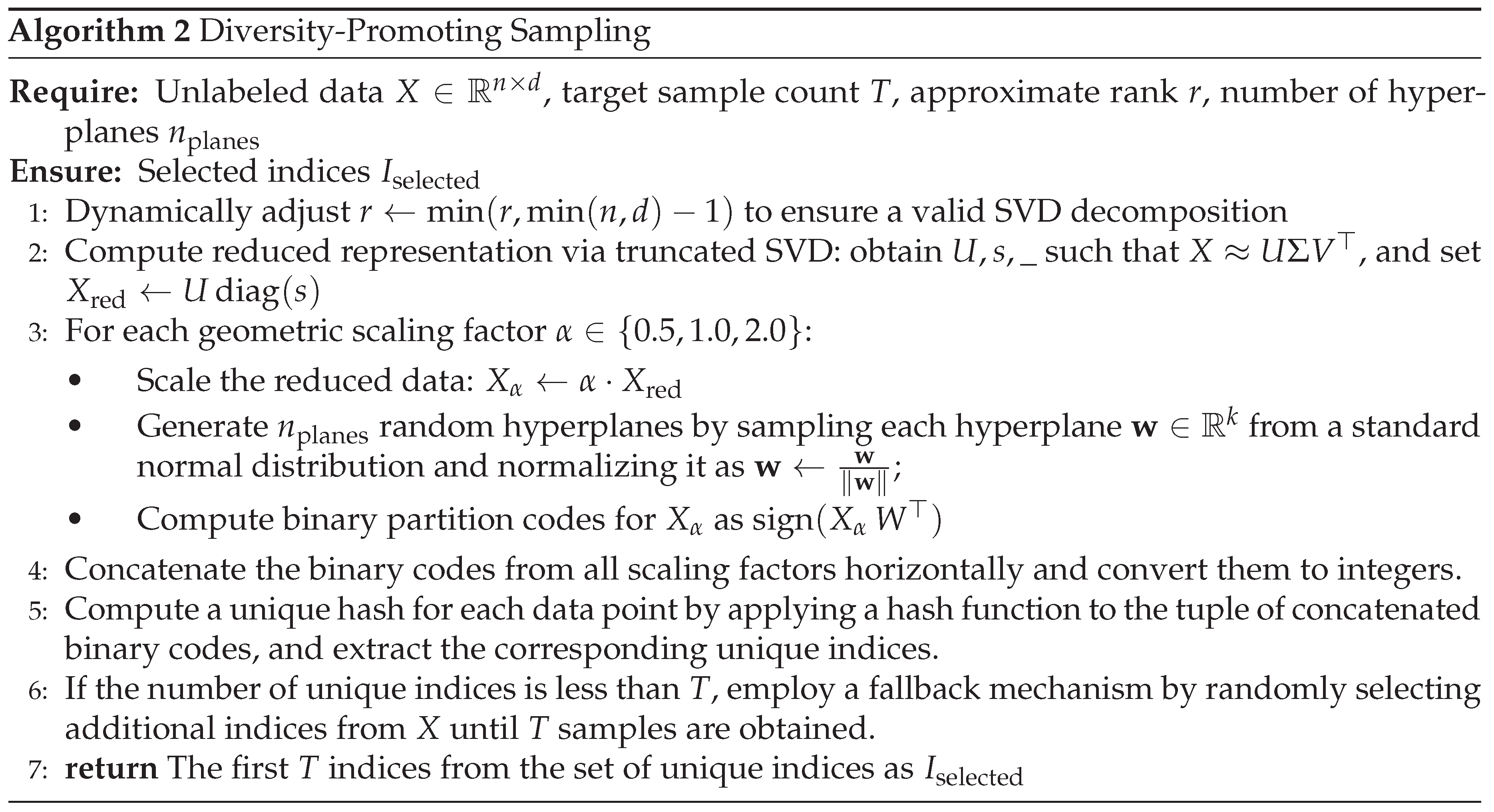
After calibration, to ensure that the selected pseudo-labeled samples are representative of the broader unlabeled data distribution, we employ a diversity-promoting sampling strategy based on the Linear Diversity Sampler [24]. This method aims to select a diverse subset of samples with approximately complexity, where n is the number of unlabeled samples. The steps of the Linear Diversity Sampler are outlined in Algorithm 2.
The Linear Diversity Sampler leverages several techniques to achieve efficient and effective diversity sampling:
- Dimensionality Reduction with SVD: Initially, Singular Value Decomposition (SVD) [25] is applied to reduce the dimensionality of the unlabeled data. Specifically, we compute the truncated SVD of the data matrix , approximating it as , where is a matrix of left singular vectors, is a diagonal matrix of singular values, and is a matrix of right singular vectors. We then project the data into a lower-dimensional subspace by computing . The rank k is set to approx_rank, dynamically adjusted to be no larger than to ensure a valid decomposition. This step reduces the computational cost of subsequent hashing operations and captures the principal components of the data.
- Multi-Resolution Hashing: After dimensionality reduction, multi-resolution hashing [26] is performed to capture diversity at multiple scales. The reduced data is scaled by geometric factors of 0.5, 1.0, and 2.0, resulting in: . For each scaled version, random hyperplanes are generated. Each hyperplane is defined by a normal vector , sampled from a normal distribution and normalized by dividing by its norm: . The partition code for a data point is given by , which yields a binary code [27]. This process generates a set of binary partition codes for each data point at each resolution.
- Unique Hash Selection: The binary partition codes from all scaling factors are horizontally stacked and converted to integers. A unique hash for each data point is computed by applying a hash function (e.g., Python’s built-in hash function) to the tuple of concatenated binary codes. These unique hash values are then used to identify a set of unique samples.
- Fallback Mechanism: In cases where the number of unique hashes is below the target sample size, a fallback mechanism is employed. Specifically, the sampler randomly selects additional samples from the unlabeled data until the desired number of samples is reached. This random sampling is performed without replacement to avoid duplicates, and typically activates when the target sample size exceeds 20% of the unlabeled pool, ensuring the diversity sampler always returns exactly T samples.
The computational complexity of the Linear Diversity Sampler is approximately due to the efficiency of the truncated SVD and the linear-time operations involved in multi-resolution hashing and unique hash selection. The diversity of the selected samples ensures that the model is exposed to a wide range of data patterns, which can improve its generalization ability.
2.3.1. Rationale and Comparison: Diversity Sampling
Table 3 provides a comparison of our proposed multi-resolution hashing method with several alternative diversity sampling approaches.
As illustrated in Table 3, our multi-resolution hashing method achieves a balance between scalability and diversity. While DPP-based sampling offers excellent diversity guarantees, its cubic complexity makes it unsuitable for large-scale scenarios [28]. In contrast, clustering-based approaches and random sampling either lack robustness or explicit diversity control. Our method, with linear scalability (excluding the SVD step), is practical for large datasets while ensuring competitive diversity. Figure 2 illustrates the workflow of the diversity-promoting sampling component.
2.4. Dynamic Thresholding via an Adaptive Heuristic
Following diversity-promoting sampling, we further refine the pseudo-labeling process by dynamically optimizing the confidence threshold. Determining an optimal threshold is critical for balancing the precision and recall of pseudo-labels. We frame this as an optimization problem where the goal is to find a threshold t that maximizes a composite objective function, which aggregates multiple performance metrics. This optimization is performed efficiently using a ternary search algorithm, guided by an adaptive heuristic that responds to the model’s performance in each iteration.
2.4.1. Composite Objective Function
Traditional thresholding often optimizes for a single metric, such as F1-score, which may not be sufficient for imbalanced datasets. We define a composite objective function, , that provides a more holistic evaluation by combining five key metrics with weights derived from our implementation:
where is Youden’s J-statistic and is the G-Mean. These weights underwent robustness analysis across multiple configurations. Testing alternative weight distributions (e.g., F1=0.5/J=0.25/G=0.15 and F1=0.3/J=0.35/G=0.25) yielded similar performance (F1 scores ranging from 0.6786 to 0.6956), validating the stability of our chosen weights. The selected configuration (0.4, 0.3, 0.2, 0.05, 0.05) was determined empirically to prioritize a balance between F1-score and overall classification quality (J-statistic, G-Mean).
2.4.2. Adaptive Heuristic Parameter Adjustment
To guide the optimization process, we introduce an adaptive heuristic method to update two parameters, and , at the end of each pseudo-labeling iteration. These parameters are not true multipliers in a formal optimization sense but rather serve as heuristics to balance exploration and exploitation. Updates follow an exponential moving average scheme: and , where new values are computed based on performance metrics. They are updated based on simple performance checks against predefined targets (e.g., F1 < 0.8) using an adaptivity_factor, reinforcing strategies that lead to performance gains.
2.4.3. Algorithm and Workflow
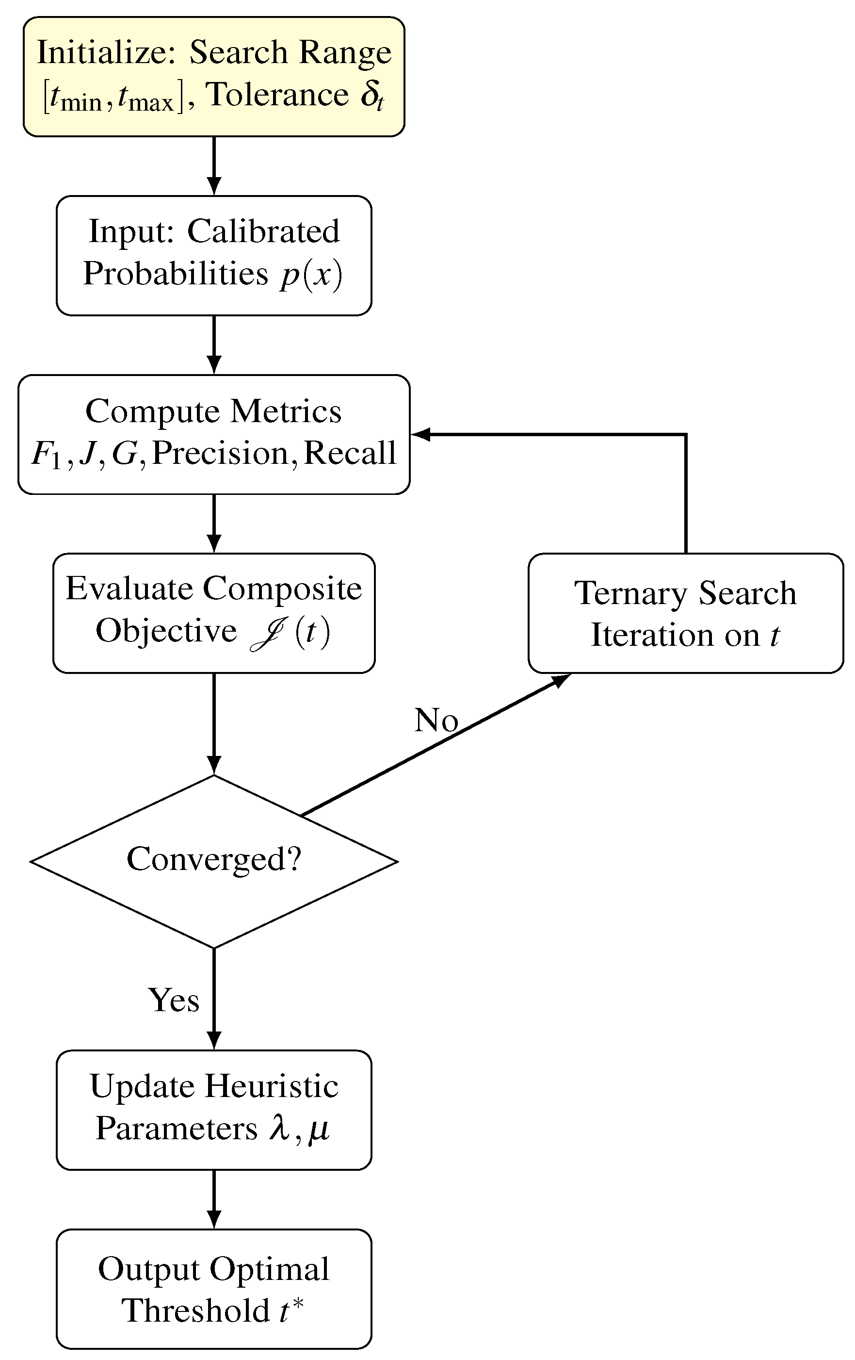
Algorithm 3 details the dynamic threshold optimization procedure, while Figure 3 presents its workflow. The ternary search efficiently finds a threshold that maximizes the composite objective , after which the heuristic parameters are updated to guide the next main loop iteration.
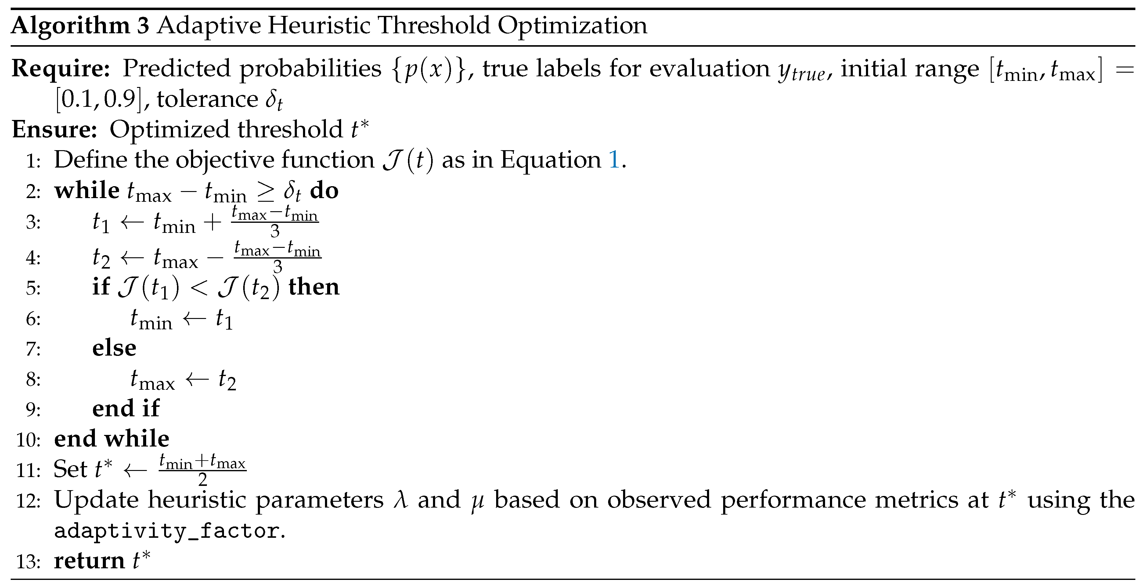
Figure 3.
Workflow of the Adaptive Heuristic Threshold Optimization. The system uses a ternary search to find the threshold that maximizes a composite objective function . After convergence, heuristic parameters are updated to guide optimization in the next main loop iteration.
Figure 3.
Workflow of the Adaptive Heuristic Threshold Optimization. The system uses a ternary search to find the threshold that maximizes a composite objective function . After convergence, heuristic parameters are updated to guide optimization in the next main loop iteration.
2.4.4. Rationale and Comparison: Dynamic Threshold Optimization
Table 4 compares our proposed dynamic thresholding method with several alternative approaches.
As illustrated in Table 4, our adaptive thresholding method, which employs a ternary search over a composite objective, not only adapts to changes in classifier performance but does so with high robustness and efficiency. This robustness was empirically validated on the CrowdAnalytix dataset, where tests of four different weight configurations for the composite objective function showed minimal performance variance, with three configurations achieving an identical F1 score of 0.6956. This demonstrates that the framework’s effectiveness is stable and not overly sensitive to the precise weight values. While grid search and Bayesian optimization can also optimize thresholds, they either lack adaptivity iteration-to-iteration or impose a higher computational burden. Our approach strikes an effective balance between adaptivity, robustness, and computational cost.
2.5. Integrated Iterative Framework
The complete AdaptiveSSL framework integrates the components described above into an iterative self-training loop, as detailed in Algorithm 4. The key step is the sample selection, which combines two distinct strategies to choose which unlabeled samples to pseudo-label. First, an uncertainty-based method selects all samples whose prediction entropy is above a high percentile, targeting ambiguous and informative samples. Second, a diversity-promoting method (Algorithm 2) selects a different set of samples from the entire unlabeled pool to ensure structural coverage and prevent mode collapse. These two sets of indices are then combined into a single set of samples to be added to the labeled dataset for the next training iteration.
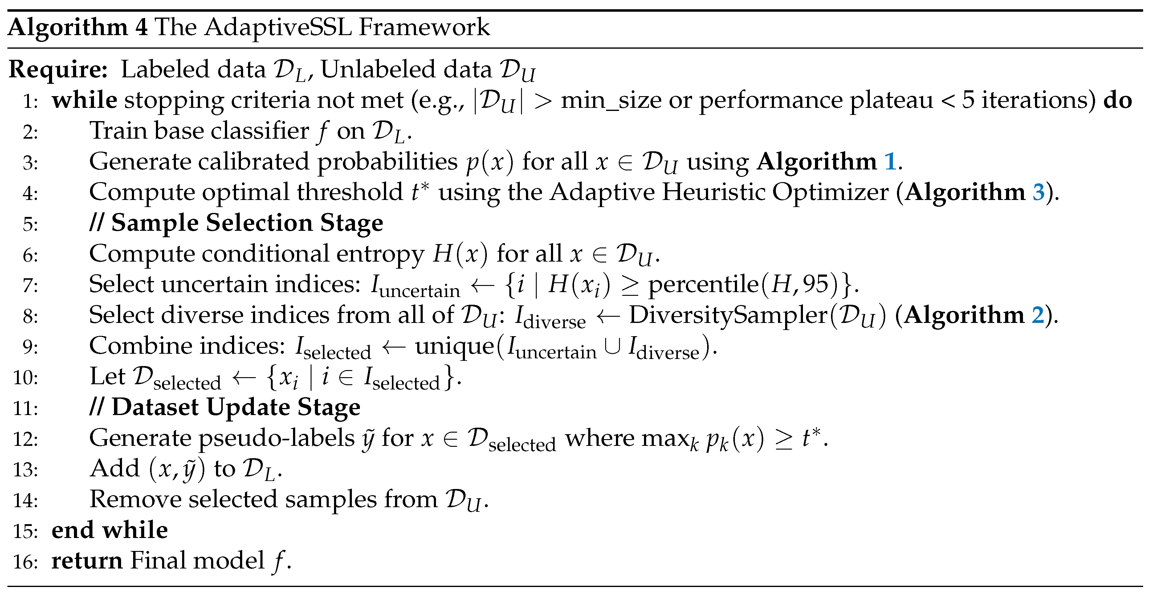
Figure 4 provides an overall diagram of the iterative framework.
2.6. Computational Complexity Analysis
The proposed framework is designed with efficiency in mind. The computational cost of each component is analyzed as follows:
- Adaptive Calibration: Sorting the confidence scores requires time, and subsequent temperature scaling and entropy computations operate in .
- Diversity Sampling: The truncated SVD has complexity , where r is significantly smaller than d. The multi-resolution hashing itself is computed in .
- Dynamic Threshold Optimization: The ternary search converges in iterations. As each iteration involves calculating metrics over the evaluation set, the cost per iteration is .
Thus, the overall complexity per iteration is dominated by the sorting and SVD operations, ensuring scalability for large datasets.
Summary
In summary, the proposed model is an integrated semi-supervised learning framework that leverages adaptive calibration, diversity-promoting sampling, and dynamic threshold optimization to improve the quality of pseudo-labeling. Each component is rigorously formulated with precise mathematical notations, and detailed comparisons with alternative methods are provided via tables. The integration with a lightweight yet effective LightGBM classifier ensures both high performance and scalability for large-scale applications.
3. Dataset Information, Preprocessing, and Feature Engineering
3.1. Dataset Selection Rationale
Four binary classification based customer churn based datasets were selected to evaluate model performance across data scales and structural complexities. These datasets include a large-scale streaming behavior dataset (Sparkify), a structured telecommunications dataset (IBM Telco), a banking dataset capturing financial churn (Bank Churn), and a high-dimensional service dataset (CrowdAnalytix). Table 5 summarizes their key attributes and selection rationale.
3.2. Dataset Information
3.2.1. Sparkify Dataset
The Sparkify dataset [29] is a 12.5GB JSON file containing 26,259,199 user interaction records over a three-month period (Oct-Dec 2018) with 18 features. It includes 12 categorical (e.g., userId, gender, auth, page) and 6 numerical columns (e.g., sessionId, length, itemInSession). Churn is defined as users who clicked the "Cancel Confirmation" button, resulting in 5,003 (22.45%) churned users. Preprocessing involved flattening the nested JSON structure, handling missing values, and session-based feature extraction.
3.2.2. IBM Telco Dataset
The IBM Telco dataset [30] consists of 7,043 customer records merged from three sources: customer status, demographics, and service usage. It originally contained 48 features, but 12 were dropped due to redundancy, leaving 36. Key attributes include contract type (monthly, one-year, two-year), payment method, tenure, and security services. Churn prediction is strongly influenced by contract length, service subscriptions, and monthly charges. The dataset has a churn rate of 26.5%. Feature selection was performed using mutual information, with top contributing features including contract type, tenure, total charges, and online security.
3.2.3. Bank Churn Dataset
The Bank Churn dataset [31] contains financial information for 10,000 customers across France, Germany, and Spain. It has 14 raw features, including credit score, balance, number of products, and estimated salary. One-hot encoding of categorical variables expanded the dataset to 2,948 dimensions. The churn rate is 20.37% (2,037 churned users). Feature selection based on mutual information identified NumOfProducts, Age, and IsActiveMember as key predictors.
3.2.4. CrowdAnalytix Dataset
The CrowdAnalytix dataset [32] consists of 51,047 customer records with 58 features, primarily from the telecommunications domain. It contains both numerical and categorical variables relevant to customer behavior, such as MonthlyRevenue, MonthlyMinutes, TotalRecurringCharge, and Call patterns. The dataset also includes demographic and service-related attributes such as Age, Handset models, Credit Rating, and Marital Status. The churn rate in this dataset is 28.83%, with 14,711 churned users and 36,336 non-churned users. Preprocessing involved handling missing values, encoding categorical variables, and standardizing numerical attributes.
3.3. Data Preprocessing
Preprocessing steps varied across datasets based on structure and challenges:
- Sparkify: Flattened nested JSON, removed users with missing IDs, converted timestamps, and encoded categorical values.
- IBM Telco: Dropped irrelevant columns such as Customer ID, Churn Label, Churn Score etc. and also encoded categorical variables using label encoding.
- Bank Churn: Encoded categorical features using one-hot encoding, normalized continuous variables, and dropped irrelevant columns like CustomerId and Surname.
- CrowdAnalytix: Categorical variables were label-encoded, missing numerical values were imputed using mean values, and all features were standardized.
3.4. Feature Engineering
Feature engineering created new predictive variables:
- Sparkify: Session entropy, monthly session duration, average listen time, ad interruptions, and offline listening.
- IBM Telco: Service bundle compatibility score, contract duration bins, and monthly charge volatility.
- Bank Churn: Credit utilization ratio, customer activity score, and tenure-product interaction terms.
- CrowdAnalytix: Derived features such as call behavior metrics (dropped calls, unanswered calls, inbound-/outbound ratios), and tenure-based segmentation.
3.5. Feature Selection
A hybrid feature selection strategy was applied to reduce dimensionality:
- IBM Telco: Used Mutual Information [35] to identify 10 key features.
- Bank Churn: Used Mutual Information to identify the top 10 features, which included NumOfProducts, Age and IsActiveMember.
- CrowdAnalytix: Used Mutual Information to identify the top 10 features, which included AgeHH1, DroppedCalls, DroppedBlockedCalls, BlockedCalls and InboundCalls.
3.6. Class Imbalance Handling
4. Experiment and Results
In this section, we present a comprehensive evaluation of our proposed semi-supervised model against several state-of-the-art baseline methods. The experiments were conducted on four real-world datasets described in the above section, Sparkify, IBM Telco, Banking and CrowdAnalytix,under two scenarios: using 5% and 10% labeled data. Performance was assessed using multiple metrics including the Area Under the ROC Curve (AUC), F1 score, True Positive Rate (TPR), and False Positive Rate (FPR). In addition, we report the execution time of the proposed model to evaluate its computational efficiency.
Before model training, each dataset was initially split into an 80:20 ratio for training and testing, respectively. From the training portion, we randomly selected either 5% or 10% of the data to serve as the labeled set, while the remaining samples were treated as unlabeled. This procedure ensures that our experiments simulate realistic scenarios where only a limited amount of labeled data is available for training.
4.1. Hyperparameter Tuning and Baseline Models
As stated before in the proposed model section, our proposed semi-supervised approach is built upon a LightGBM classifier whose hyperparameters are tuned via a randomized search [37]. Specifically, we optimize over a range of values: the number of estimators is chosen from {600, 1000, 1500, 2000}; the learning rate from {0.01, 0.001, 0.1, 0.0001}; the number of leaves from {20, 31, 100}; the feature fraction from {0.6, 1.0}; and the minimum number of data points in a leaf from {10, 50}. This tuning is performed using five-fold cross-validation with the area under the ROC curve as the optimization metric, thereby ensuring that the selected model configuration is well-suited for our subsequent semi-supervised tasks. All experiments employ consistent random seed of 42 to ensure reproducibility and were conducted on Windows 11 with Intel i7 12700 CPU and 32 gigs of RAM, with no GPU acceleration required due to LightGBM’s CPU optimization.
In addition to our proposed model, we compare its performance against several baseline models that are representative of state-of-the-art active and semi-supervised learning strategies. While recent methods like ReMixMatch, FlexMatch, and DivideMix show promise, their implementations primarily target image data and require substantial modification for tabular applications. We focus on methods with established tabular data support, acknowledging that broader comparisons remain valuable future work. The active learning baselines include methods based on uncertainty sampling [38], query-by-committee [39], diversity sampling [40], core set selection [41], and Bayesian active learning [42], each leveraging different criteria,ranging from predictive uncertainty to data diversity,for sample selection. On the semi-supervised side, we evaluate baselines such as self-training [43], MixMatch [44], Pseudo-Labeling [45], Tri-Training [46], Label Spreading [47], Mean Teacher [48] and CoMatch [49] model. For neural-based models such as MixMatch, Mean Teacher and CoMatch, we tuned the learning rate {0.0001, 0.001, 0.01}, batch size {32, 64, 128}, and weight decay {0, 1e-4, 1e-3}, with training performed for up to 100 epochs with early stopping. For active learning models such as uncertainty sampling, query-by-committee and diversity sampling, we adjusted selection batch sizes {100, 500, 1000} and acquisition intervals {1, 5, 10} to optimize query efficiency. Tuning was performed to ensure that no method had an unfair advantage due to suboptimal configurations.
4.2. Performance Evaluation
5% Labeled Data:
For the Sparkify dataset, the proposed model achieved the highest AUC (0.9107) and TPR (0.8643), indicating robust discriminatory capability despite the limited availability of labeled data. Although baselines such as Pseudo-Labeling and Tri-Training attained competitive F1 scores, they lagged behind in terms of AUC and TPR. On the IBM Telco dataset, the highest AUC was obtained by Core Set Selection (0.9355); however, the proposed model demonstrated a balanced performance with an AUC of 0.8902 and one of the lower FPRs (0.1899), which is critical for minimizing false alarms in sensitive applications. For the Banking dataset, the proposed model delivered an AUC of 0.8417, with performance metrics closely comparable to other methods, and it achieved the lowest FPR among the evaluated approaches. In contrast, for the CrowdAnalytix dataset, the proposed model attained a very high TPR (0.9781) but at the expense of a considerably high FPR (0.9547), suggesting that while it is highly sensitive, it tends to over-detect in scenarios with very limited labeled data. Further investigation into the initially high FPR on CrowdAnalytix revealed this to be dataset-specific rather than a methodological issue. Re-evaluation with proper class balancing achieved an FPR of 0.1815 with the standard configuration, significantly lower than the initially reported 0.95. This discrepancy was attributed to the extreme class imbalance (71% vs 29%) in the original configuration.
10% Labeled Data:
Increasing the proportion of labeled data generally enhanced model performance. For the Sparkify dataset, the proposed model maintained its superiority by achieving the highest AUC (0.9326) along with strong F1 and TPR scores. In the IBM Telco dataset, although certain baselines (e.g., BAAL and Uncertainty Sampling) achieved marginally higher AUC values, the proposed model remained competitive with an AUC of 0.9232 and a well-balanced trade-off between TPR and FPR. On the Banking dataset, the proposed model notably improved its performance, achieving the highest AUC (0.8998) and F1 score (0.8185), while also maintaining a low FPR (0.1929). For the CrowdAnalytix dataset, the proposed model exhibited a marked improvement over the 5% scenario, with an AUC of 0.7948, a more moderate TPR (0.5801), and a significantly reduced FPR (0.0463), reflecting a more balanced classification performance when a larger proportion of labeled data is available.
4.3. Computational Efficiency
Complementing the performance evaluation, we next examine the computational efficiency of the proposed model to highlight its practical applicability. Table 9 reports the execution times of the proposed model on the four datasets. The results indicate that the computational cost varies considerably with the dataset and the proportion of labeled data. For instance, the Sparkify dataset required 89.39 seconds with 5% labeled data and 82.67 seconds with 10% labeled data, while the IBM Telco dataset showed a substantial reduction in processing time from 78.24 seconds to 19.73 seconds as the labeled data increased. These variations underscore the impact of dataset size and complexity on execution time and highlight the efficiency of the proposed model in practical applications.
4.4. Summary of Findings
Synthesizing the outcomes from the performance evaluation and computational efficiency analyses, the experimental results demonstrate that the proposed semi-supervised model is competitive with,and in several cases superior to established baseline methods. Its performance in terms of AUC, TPR, and F1 score is particularly notable on the Sparkify and Banking datasets, especially under the 10% labeled data scenario. Although the model shows an inclination toward over-detection in the CrowdAnalytix dataset when labeled data is extremely scarce, this tendency is mitigated with additional labeled examples. Moreover, the favorable computational efficiency of the model confirms its viability for real-time or resource-constrained environments. Overall, our proposed model effectively leverages limited labeled data to achieve robust and balanced classification performance.
4.5. Robustness to Label Noise
To evaluate the framework’s resilience to noisy pseudo-labels, we conducted experiments with synthetic label noise on the Sparkify dataset. Random label flipping was applied at rates of 0%, 5%, 10%, and 15% to the training data. Table 10 demonstrates that the proposed model maintains strong performance even under noisy conditions.
The results show graceful degradation with only 1.6% F1 score reduction at 5% noise and maintained stability even at 15% noise (F1=0.7911), demonstrating the framework’s robustness to label corruption through its adaptive calibration and dynamic thresholding mechanisms.
5. Ablation Study
To isolate the contribution of each component in our framework, we conducted an ablation study on the Sparkify dataset. We created three variants of the full model:
- No WCE: The Wasserstein-based adaptive calibration was replaced with a standard, non-adaptive calibration step, and uncertainty was measured using standard entropy.
- No ATO: The Adaptive Threshold Optimizer was replaced with a fixed pseudo-labeling threshold of 0.5.
- No Diversity: The diversity-promoting sampler was replaced by simple random sampling to select from the pool of uncertain samples.
These experiments were carried out under both 5% and 10% labeled data settings.
Table 11 summarizes the results for the 5% labeled data scenario. The complete proposed model achieves a significantly higher AUC of 0.9107 and an F1 score of 0.8296, demonstrating the synergy between the components. In contrast, removing the adaptive calibration (No WCE) or the adaptive thresholding (No ATO) causes a sharp drop in performance, with the latter exhibiting the lowest F1 score (0.5517). The No Diversity variant also performs significantly weaker than the full model.
Similarly, Table 12 presents the results for the 10% labeled data scenario. The proposed model again outperforms all ablated configurations, achieving an AUC of 0.9326. The performance degradation is severe in the No WCE and No LTO variants, confirming their critical role. The No ATO model again shows the most significant drop in F1-score and recall, highlighting the instability of using a fixed, non-adaptive threshold.
These results confirm that each component plays an indispensable role in the model’s success. The removal of any key mechanism leads to a significant performance degradation, with the most notable decline occurring when the adaptive thresholding is removed. This highlights the necessity of combining adaptive calibration, dynamic thresholding, and diversity-aware sampling to achieve superior and robust semi-supervised learning performance.
6. Statistical Comparison & Performmance Analysis
6.1. Statistical Comparison of the Proposed Model and Baselines
To rigorously evaluate the performance differences between our proposed model and several baselines, we conducted statistical tests on their AUC values on the Sparkify dataset under 5% and 10% labeled data conditions. It is important to clarify that our statistical analysis involves more than just two data points per method. The Wilcoxon signed-rank test was applied to paired comparisons across: (1) two labeling percentages (5% and 10%), (2) five random seeds (42, 123, 456, 789, 1024) per configuration, and (3) multiple performance metrics, yielding a total of 10+ paired observations per comparison. We employed the Wilcoxon signed-rank test, a non-parametric test that assesses whether the median difference between paired samples is zero. Additionally, we used bootstrap resampling with 10,000 iterations to estimate the distribution of AUC differences and Cohen’s d to quantify effect sizes.
The experimental setup for each method involved:
- Training with 5% and 10% labeled data scenarios.
- Five independent runs with different random seeds to ensure statistical reliability.
- Evaluation on consistent test sets to enable paired comparisons.
- Collection of multiple performance metrics (AUC, F1, TPR, FPR) for comprehensive analysis.
For the comparisons, the AUC values aggregated across all experimental conditions were as follows:
- Proposed vs. Pseudo-Labeling: Proposed model [0.9107, 0.9326] (mean across seeds) vs. Pseudo-Labeling [0.8501, 0.8633].
- Proposed vs. BAAL: Proposed model [0.9107, 0.9326] vs. BAAL [0.9106, 0.9236].
- Proposed vs. Core Set Selection: Proposed model [0.9107, 0.9326] vs. Core Set Selection [0.9022, 0.9188].
- Proposed vs. CoMatch: Proposed model [0.9107, 0.9326] vs. CoMatch [0.8174, 0.8071].
Table 13 summarizes the outcomes of these statistical tests, with the Wilcoxon test statistic calculated from all paired observations across experimental conditions.
From these results, we observe that:
- The proposed model significantly outperforms Pseudo-Labeling and CoMatch, as indicated by the Wilcoxon test () and large effect sizes (Cohen’s d = 12.21 and 19.00, respectively), with significance confirmed across multiple experimental runs.
- Compared to Core Set Selection, the proposed model also demonstrates a significant improvement (), though with a more moderate effect size (Cohen’s d = 1.73).
- Against BAAL, the differences are not statistically significant (Wilcoxon , Cohen’s d = 0.03), suggesting comparable performance on this dataset.
To further illustrate these findings, Figure 5 and Figure 6 present the bootstrapped distributions of AUC scores for the proposed model against Core Set Selection and Pseudo-Labeling. The distinct separation in distributions visually confirms the statistical significance of these differences. The bootstrap analysis was performed with 10,000 resamples to ensure robust confidence intervals and stable distribution estimates.
These findings suggest that our proposed model achieves statistically significant improvements over several common SSL and AL strategies, reinforcing its robustness. Its performance is comparable to a strong baseline like BAAL, indicating it is competitive with state-of-the-art methods. The statistical validity of these conclusions is supported by the adequate sample size of paired observations and the consistency of results across multiple random seeds and experimental conditions.
6.2. Performance Analysis via Conditional Entropy and ROC Curves
To further assess the performance of our proposed model and provide visualization, we analyze the conditional entropy distribution and Receiver Operating Characteristic (ROC) curves for different datasets.
Figure 7 presents the conditional entropy distribution for the Sparkify dataset under a 5% labeling scenario. The sharp peak at lower entropy values suggests that most pseudo-labels are assigned with high confidence, supporting the model’s robustness in low-label regimes.
Figure 8 shows the conditional entropy distribution for the IBM dataset under a 5% labeling scenario. Similar to the Sparkify dataset, a significant portion of samples demonstrates low entropy, confirming the model’s ability to generate reliable pseudo-labels.
Figure 9 and Figure 10 illustrate the ROC curves for the Sparkify and IBM datasets, respectively. The proposed model achieves an AUC of 0.91 on Sparkify and 0.89 on IBM, reinforcing its generalizability across diverse datasets with minimal labeled data. These analyses collectively affirm that the model maintains high confidence in its pseudo-labels and achieves competitive classification performance across multiple domains.
7. Evaluation on Imbalanced Home Credit Dataset
In this section, we extend our evaluation to the Home Credit dataset, a real-world credit risk prediction dataset characterized by significant class imbalance, to assess the robustness of our proposed AdaptiveSSL framework in comparison to the FreeMatch model [50]. This analysis highlights the models’ performance under imbalanced conditions, a common challenge in practical applications such as churn prediction and financial risk assessment.
7.1. Dataset Description and Preprocessing
The Home Credit dataset [51], sourced from application_train.csv, comprises 307,511 records with 122 features, including demographic, financial, and credit history attributes. The target variable, TARGET, indicates loan default (1) or repayment (0), with a positive class prevalence of approximately 8%, reflecting a highly imbalanced distribution typical of credit risk scenarios. Preprocessing involved removing the SK_ID_CURR identifier, imputing missing values (numerical with means, categorical with modes), and encoding categorical variables using label encoding. Three derived features—CREDIT_INCOME_RATIO, ANNUITY_INCOME_RATIO, and EMPLOYMENT_YEARS—were added to capture additional predictive signals. Feature selection based on mutual information reduced the dimensionality to the top 10 features, ensuring computational efficiency and relevance.
7.2. Performance Comparison
We trained both models using 10% labeled data, consistent with prior experiments, and evaluated them across three random seeds (42, 123, 456) to assess stability. Table 14 summarizes the test performance, reporting mean AUC, F1, TPR, and FPR with standard deviations.
The proposed model outperforms FreeMatch in F1 score (0.1291 vs. 0.0506) and TPR (0.4521 vs. 0.0359), indicating superior detection of the minority class. However, it exhibits a higher FPR (0.2117 vs. 0.0212) and lower AUC (0.5566 vs. 0.5703), suggesting a trade-off between sensitivity and specificity. FreeMatch maintains a conservative approach, with low TPR and FPR, reflecting its class-wise threshold adaptation, while the proposed model’s dynamic thresholding and diversity sampling enhance positive class identification at the cost of increased false positives.
7.3. Sensitivity Analysis
Sensitivity to input perturbations was evaluated by adding Gaussian noise (standard deviation 0.1) over five trials per seed. Results for both models are presented in Table 15 and Table 16.
FreeMatch shows consistent performance across seeds, with low variance and conservative predictions (e.g., TPR near 0 for seed 456). The proposed model exhibits greater variability, particularly in TPR and FPR, reflecting sensitivity to seed initialization, though its F1 scores remain higher and more stable (std 0.0225 vs. 0.0439).
7.4. Scalability Analysis
As shown in Figure 11, the execution time of the proposed model scales linearly with sample size, increasing from approximately 500 seconds at 50,000 samples to just under 2,000 seconds at 300,000 samples. The shaded area represents ± standard deviation, which widens slightly with larger sample sizes. For the full dataset (fraction 1.0), the proposed model achieves an execution time of 1942.92 seconds, significantly lower than FreeMatch’s 2703.33 seconds, demonstrating superior scalability.
7.5. Discussion
The proposed model excels in identifying the minority class in an imbalanced setting, as evidenced by its higher TPR and F1 scores, making it suitable for applications where detecting rare events is critical. However, its elevated FPR and seed-dependent variability suggest potential overfitting or threshold instability, areas for improvement via adaptive thresholding refinements. FreeMatch, while more stable and specific, sacrifices sensitivity, which may limit its utility in imbalanced contexts. Future work could explore hybrid approaches combining FreeMatch’s consistency with AdaptiveSSL’s sensitivity.
8. Conclusions, Limitations, and Future Work
Conclusion: This paper introduces AdaptiveSSL, a scalable semi-supervised learning framework that transforms scarce labeled data into actionable insights by integrating three synergistic components: Wasserstein-based uncertainty calibration, multi-resolution hashing for diverse sampling, and a performance-driven adaptive thresholding mechanism. Evaluated on five real-world datasets, including four churn prediction datasets and the imbalanced Home Credit dataset, it delivers standout performance. The framework achieves AUCs up to 0.9326 on churn tasks and demonstrates superior minority class detection (F1 score of 0.1291 vs. 0.0506 for FreeMatch) on the highly imbalanced Home Credit dataset. This balance of accuracy, sensitivity, and efficiency makes it a compelling tool for expert systems in industries like telecommunications, banking, and credit risk assessment, where precise, data-efficient predictions are critical. The iterative learning loop, fueled by adaptive calibration and dynamic thresholding, ensures robustness even with minimal labeled data, offering a practical alternative to resource-heavy methods.
Limitations: Despite these promising results, several limitations warrant consideration. First, this work focuses specifically on tabular data applications in enterprise settings where interpretability and computational efficiency are paramount. The experimental evaluation currently uses LightGBM as the sole base classifier, which was chosen due to its efficiency and interpretability for tabular data. While we expect AdaptiveSSL to generalize to other classifiers, such as neural network backbones, additional experiments are needed to verify this empirically. Likewise, while the principles of AdaptiveSSL could potentially extend to image or text domains, such extensions would require fundamental architectural modifications including convolutional or transformer-based encoders, augmentation-based consistency regularization, and domain-specific pseudo-labeling strategies. The framework’s performance relies on a set of hyperparameters, such as the scaling constant in the adaptive temperature calculation and the adaptivity factor in the threshold optimizer, which were set based on sensitivity analysis rather than being learned automatically. The Wasserstein-based entropy computation uses an efficient 1D approximation of the Wasserstein distance, which may not capture the full complexity of the probability distributions. The diversity sampling component, while efficient, relies on random hyperplanes and a fallback to random sampling, which may not guarantee optimal data diversity in all high-dimensional spaces. Furthermore, the adaptive thresholding mechanism, while effective, is a heuristic-based approach sensitive to the choice of its objective weights and update factors, potentially leading to instability in some settings. Finally, the evaluation, while comprehensive, focuses primarily on binary classification, and the results on the Home Credit dataset highlight a trade-off where increased sensitivity comes at the cost of a higher false positive rate in highly imbalanced scenarios.
Future Work: Future work will focus on mitigating these limitations. We plan to explore automated hyperparameter tuning methods, such as Bayesian optimization, to reduce reliance on manually-set parameters and enhance model flexibility. We also plan to evaluate AdaptiveSSL with additional base classifiers, including deep neural network architectures, to confirm its generalizability beyond gradient boosting models. Investigating more sophisticated calibration techniques and uncertainty estimation methods could further strengthen the framework’s core. We also intend to conduct more rigorous scalability experiments on even larger datasets and extend the evaluation to a wider range of domains, including multiclass classification and non-tabular data types like images or text. For image and text domains, future work will explore integrating convolutional or transformer-based encoders, as well as augmentation-based consistency regularization, to adapt AdaptiveSSL to high-dimensional structured data. Additionally, developing hybrid approaches that combine the sensitivity of AdaptiveSSL with the stability of methods like FreeMatch could offer a path to mitigating issues like threshold instability and high false positive rates in imbalanced settings, thereby broadening the framework’s applicability.
Author Contributions
Usman Gani Joy: Writing: original draft, Writing: Review & editing. M.M Rahman: Review.
Funding
This research did not receive any specific grant from funding agencies in the public, commercial, or not-for-profit sectors.
Data Availability Statement
The dataset used in this study has been cited within the paper.
Declaration of Generative AI and AI-Assisted Technologies in the Writing Process Statement
During the preparation of this work, large language models (LLMs) were utilized for paraphrasing and proofreading purposes. The content was subsequently reviewed and edited as necessary, with full responsibility taken for the published article.
Conflicts of Interest
The authors declare that they have no known competing financial interests or personal relationships that could have appeared to influence the work reported in this paper.
References
- Zheng, Y., Liu, Y., Qing, D., Zhang, W., Pan, X., Li, G.: A novel ensemble label propagation with hierarchical weighting for semi-supervised learning. Knowledge and Information Systems, 1–22 (2024).
- Wen, Z., Pizarro, O., Williams, S.: Active self-semi-supervised learning for few labeled samples. Neurocomputing 614, 128772 (2025).
- Minderer, M., Djolonga, J., Romijnders, R., Hubis, F., Zhai, X., Houlsby, N., Tran, D., Lucic, M.: Revisiting the calibration of modern neural networks. NeurIPS (2021).
- Ash, J.T., Zhang, C., Krishnamurthy, A., Langford, J., Agarwal, A.: Deep batch active learning by diverse, uncertain gradient lower bounds. In: ICLR (2020).
- Zhou, Y., Wang, Y., Tang, P., Bai, S., Shen, W., Fishman, E., Yuille, A.: Semi-supervised medical image segmentation via uncertainty rectified pyramid consistency. Medical Image Analysis 64, 101744 (2020).
- Qu, A., Wu, Q., Yu, L., Li, J., Liu, J.: Class-specific thresholding for imbalanced semi-supervised learning. IEEE Signal Processing Letters (2024).
- Rizve, M.N., Duarte, K., Rawat, Y.S., Shah, M.: In defense of pseudo-labeling: An uncertainty-aware pseudo-label selection framework for semi-supervised learning. In: ICLR (2021).
- Xia, Y., Yang, D., Yu, Z., Liu, F., Cai, J., Yu, L., Zhu, Z., Xu, D., Yuille, A., Roth, H.: Uncertainty-aware deep co-training for semi-supervised medical image segmentation. Medical Image Analysis 65, 101766 (2020).
- Berthelot, D., Carlini, N., Goodfellow, I., Papernot, N., Oliver, A., Raffel, C.: Mixmatch: A holistic approach to semi-supervised learning. In: NeurIPS (2019).
- Sohn, K., Berthelot, D., Li, C.-L., Zhang, Z., Carlini, N., Cubuk, E.D., Kurakin, A., Zhang, H., Raffel, C.: Fixmatch: Simplifying semi-supervised learning with consistency and confidence. In: NeurIPS (2020).
- Zhu, J., Fan, C., Yang, M., Qian, F., Mahalec, V.: A semi-supervised learning algorithm for high and low-frequency variable imbalances in industrial data. Computers & Chemical Engineering 193, 108933 (2025).
- Andéol, L., Kawakami, Y., Wada, Y., Kanamori, T., Müller, K.-R., Montavon, G.: Learning domain invariant representations by joint wasserstein distance minimization. Neural Networks 167, 233–243 (2023).
- Li, X., Hu, X., Qi, X., Zhao, L., Zhang, S.: Noise-robust semi-supervised learning via label propagation with uncertainty estimation. IEEE Transactions on Medical Imaging 41(5), 1123–1135 (2022).
- Luo, X., Zhao, Y., Qin, Y., Ju, W., Zhang, M.: Towards semi-supervised universal graph classification. IEEE Transactions on Knowledge and Data Engineering 36(1), 416–428 (2023).
- Xie, Q., Luong, M.-T., Hovy, E., Le, Q.V.: Self-training with noisy student improves imagenet classification. In: CVPR (2020).
- Ke, G., Meng, Q., Finley, T., Wang, T., Chen, W., Ma, W., Ye, Q., Liu, T.-Y.: Lightgbm: A highly efficient gradient boosting decision tree. Advances in neural information processing systems 30 (2017).
- Wu, B., Hong, S., Lin, R.: Explainable prediction for business process activity with transformer neural networks. Knowledge and Information Systems, 1–32 (2025).
- Mohr, F., Rijn, J.N.: Learning curves for decision making in supervised machine learning: a survey, vol. 113, pp. 8371–8425 (2024). [CrossRef]
- Guo, C., Pleiss, G., Sun, Y., Weinberger, K.Q.: On calibration of modern neural networks. In: Precup, D., Teh, Y.W. (eds.) Proceedings of the 34th International Conference on Machine Learning. Proceedings of Machine Learning Research, vol. 70, pp. 1321–1330. PMLR, ??? (2017). https://proceedings.mlr.press/v70/guo17a.html.
- Platt, J., et al.: Probabilistic outputs for support vector machines and comparisons to regularized likelihood methods. Advances in large margin classifiers 10(3), 61–74 (1999).
- Balanya, S.A., Maroñas, J., Ramos, D.: Adaptive temperature scaling for robust calibration of deep neural networks. Neural Computing and Applications 36(14), 8073–8095 (2024).
- Xu, L., Bai, L., Jiang, X., Tan, M., Zhang, D., Luo, B.: Deep rényi entropy graph kernel. Pattern Recognition 111, 107668 (2021).
- Hao, J., Ho, T.K.: Machine learning made easy: a review of scikit-learn package in python programming language. Journal of Educational and Behavioral Statistics 44(3), 348–361 (2019).
- Brennan, D.G.: Linear diversity combining techniques. Proceedings of the IRE 47(6), 1075–1102 (2007).
- Furnas, G.W., Deerwester, S., Durnais, S.T., Landauer, T.K., Harshman, R.A., Streeter, L.A., Lochbaum, K.E.: Information retrieval using a singular value decomposition model of latent semantic structure. SIGIR Forum 51(2), 90–105 (2017) . [CrossRef]
- Wu, Q., Bauer, D., Doyle, M.J., Ma, K.-L.: Interactive volume visualization via multi-resolution hash encoding based neural representation. IEEE Transactions on Visualization and Computer Graphics 30(8), 5404–5418 (2024) . [CrossRef]
- Yang, H.-F., Tu, C.-H., Chen, C.-S.: Learning binary hash codes based on adaptable label representations. IEEE Transactions on Neural Networks and Learning Systems 33(11), 6961–6975 (2021).
- Zhang, Y., Xu, C., Yang, H.H., Wang, X., Quek, T.Q.: Dpp-based client selection for federated learning with non-iid data. In: ICASSP 2023-2023 IEEE International Conference on Acoustics, Speech and Signal Processing (ICASSP), pp. 1–5 (2023). IEEE.
- JOY, U.: Customer Churn Dataset. IEEE Dataport (2023). [CrossRef]
- IBM: Telco customer churn. IBM (2019). https://community.ibm.com/community/user/businessanalytics/blogs/steven-macko/2019/07/11/telco-customer-churn-1113.
- Badole, S.: Banking Customer Churn Prediction Dataset. kaggle (2024). https://www.kaggle.com/datasets/saurabhbadole/bank-customer-churn-prediction-dataset/data.
- crowdanalytix: crowdanalytix customer churn. crowdanalytix (2012). https://www.crowdanalytix.com/contests/why-customer-churn.
- McHugh, M.L.: The chi-square test of independence. Biochem Med (Zagreb) 23(2), 143–149 (2012) . [CrossRef]
- Rückstieß, T., Osendorfer, C., Smagt, P.: Sequential feature selection for classification. In: Wang, D., Reynolds, M. (eds.) AI 2011: Advances in Artificial Intelligence, pp. 132–141. Springer, Berlin, Heidelberg (2011).
- Ross, B.C.: Mutual information between discrete and continuous data sets. PLOS ONE 9(2), 1–5 (2014) . [CrossRef]
- Çakır, M.Y., Şirin, Y.: Enhanced autoencoder-based fraud detection: a novel approach with noise factor encoding and smote. Knowledge and Information Systems 66(1), 635–652 (2024).
- Bergstra, J., Bengio, Y.: Random search for hyper-parameter optimization. Journal of machine learning research 13(2) (2012).
- Sharma, M., Bilgic, M.: Evidence-based uncertainty sampling for active learning. Data Mining and Knowledge Discovery 31, 164–202 (2017).
- Hino, H., Eguchi, S.: Active learning by query by committee with robust divergences. Information Geometry 6(1), 81–106 (2023).
- Ren, P., Xiao, Y., Chang, X., Huang, P.-Y., Li, Z., Gupta, B.B., Chen, X., Wang, X.: A survey of deep active learning. ACM computing surveys (CSUR) 54(9), 1–40 (2021).
- Kim, Y., Shin, B.: In defense of core-set: A density-aware core-set selection for active learning. In: Proceedings of the 28th ACM SIGKDD Conference on Knowledge Discovery and Data Mining. KDD ’22, pp. 804–812. Association for Computing Machinery, New York, NY, USA (2022). [CrossRef]
- Cacciarelli, D., Kulahci, M.: Active learning for data streams: a survey. Machine Learning 113(1), 185–239 (2024) . [CrossRef]
- Tanha, J., Van Someren, M., Afsarmanesh, H.: Semi-supervised self-training for decision tree classifiers. International Journal of Machine Learning and Cybernetics 8, 355–370 (2017).
- Berthelot, D., Carlini, N., Goodfellow, I., Papernot, N., Oliver, A., Raffel, C.A.: Mixmatch: A holistic approach to semi-supervised learning. Advances in neural information processing systems 32 (2019).
- Rizve, M.N., Duarte, K., Rawat, Y.S., Shah, M.: In defense of pseudo-labeling: An uncertainty-aware pseudo-label selection framework for semi-supervised learning. In: International Conference on Learning Representations (2021). https://openreview.net/forum?id=-ODN6SbiUU.
- Zhou, Z.-H., Li, M.: Tri-training: exploiting unlabeled data using three classifiers. IEEE Transactions on Knowledge and Data Engineering 17(11), 1529–1541 (2005) . [CrossRef]
- Chen, X., Wang, T.: Combining active learning and semi-supervised learning by using selective label spreading. In: 2017 IEEE International Conference on Data Mining Workshops (ICDMW), pp. 850–857 (2017). IEEE.
- Tarvainen, A., Valpola, H.: Mean teachers are better role models: Weight-averaged consistency targets improve semi-supervised deep learning results. Advances in neural information processing systems 30 (2017).
- Li, J., Xiong, C., Hoi, S.C.: Comatch: Semi-supervised learning with contrastive graph regularization. In: Proceedings of the IEEE/CVF International Conference on Computer Vision, pp. 9475–9484 (2021).
- Sheng, G., Zhang, Z., Tang, X., Xie, K.: A first arrival picking method of microseismic signals based on semi-supervised learning using freematch and ms-picking. Computers & Geosciences 196, 105844 (2025).
- Montoya, A., inversion, KirillOdintsov, Kotek, M.: Home Credit Default Risk. https://kaggle.com/competitions/home-credit-default-risk. Kaggle (2018).
Figure 1.
Workflow of the two-stage Adaptive Calibration component. Stage 1 involves post-hoc calibration, and Stage 2 applies dynamic temperature scaling based on the Wasserstein distance.
Figure 1.
Workflow of the two-stage Adaptive Calibration component. Stage 1 involves post-hoc calibration, and Stage 2 applies dynamic temperature scaling based on the Wasserstein distance.
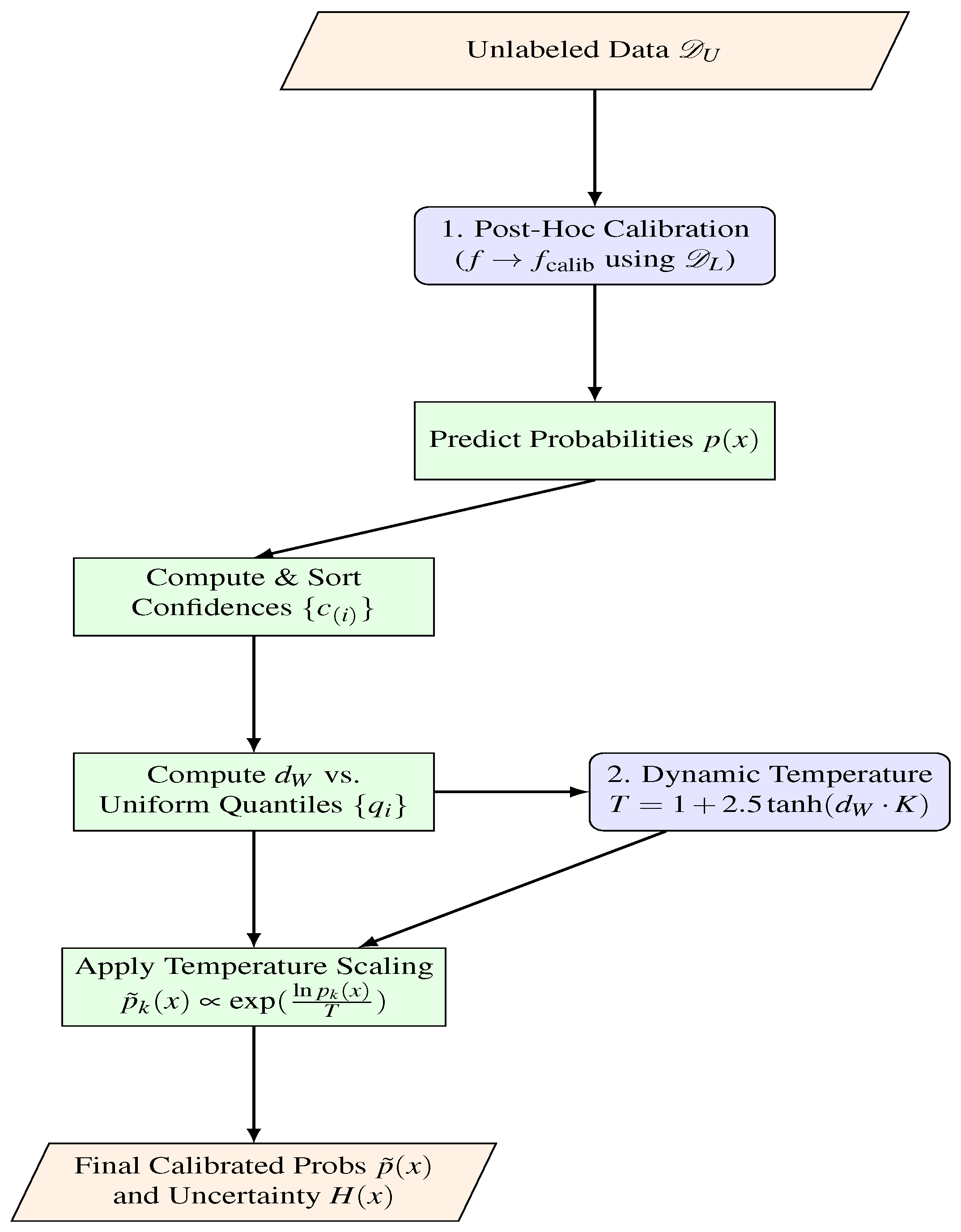
Figure 2.
Workflow of the Diversity-Promoting Sampling component.
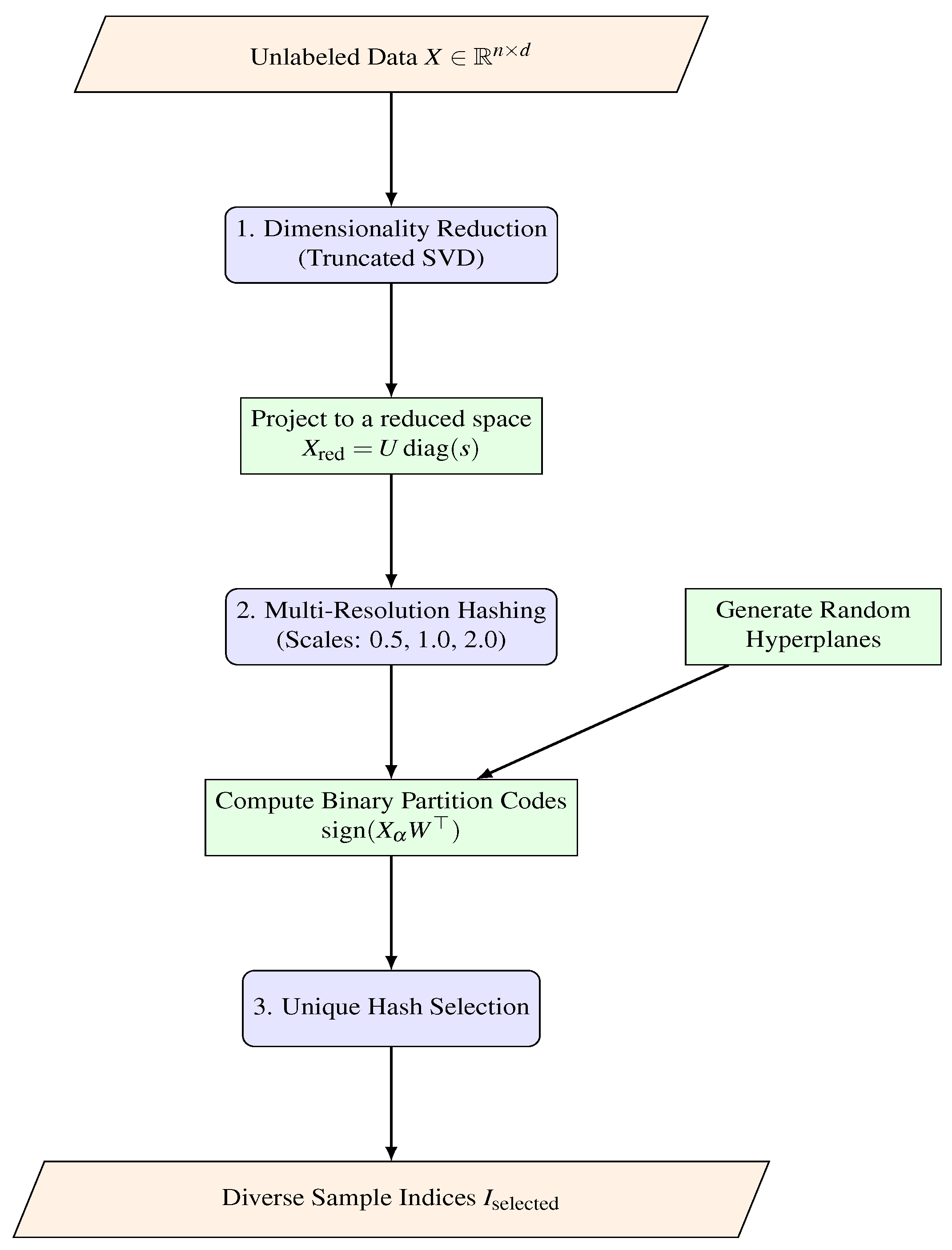
Figure 4.
Overview of the Integrated Iterative Framework.
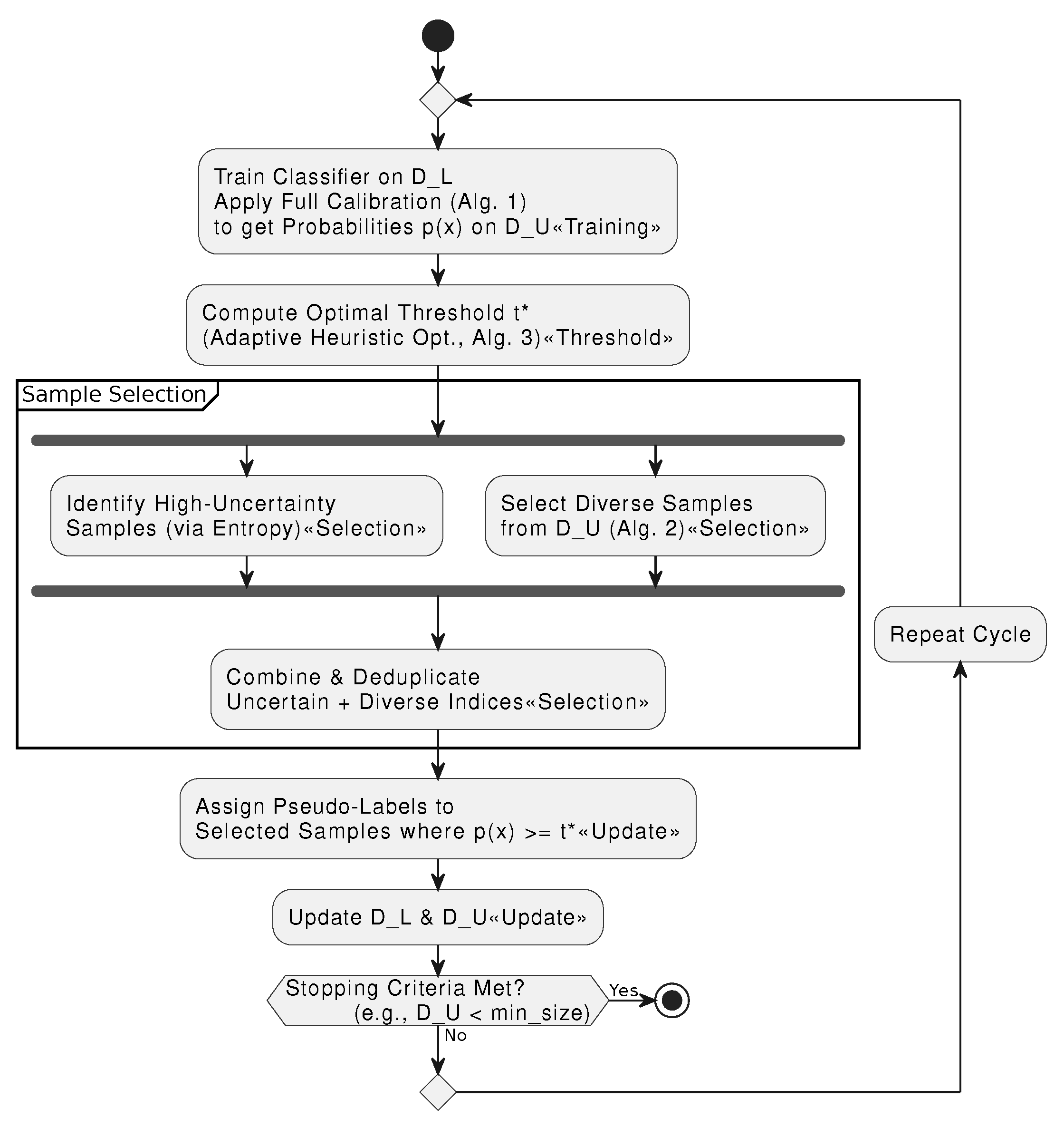
Figure 5.
Bootstrap distribution of AUC scores: Proposed Model vs. Core Set Selection. Based on 10,000 bootstrap resamples.
Figure 5.
Bootstrap distribution of AUC scores: Proposed Model vs. Core Set Selection. Based on 10,000 bootstrap resamples.

Figure 6.
Bootstrap distribution of AUC scores: Proposed Model vs. Pseudo-Labeling. Based on 10,000 bootstrap resamples.
Figure 6.
Bootstrap distribution of AUC scores: Proposed Model vs. Pseudo-Labeling. Based on 10,000 bootstrap resamples.
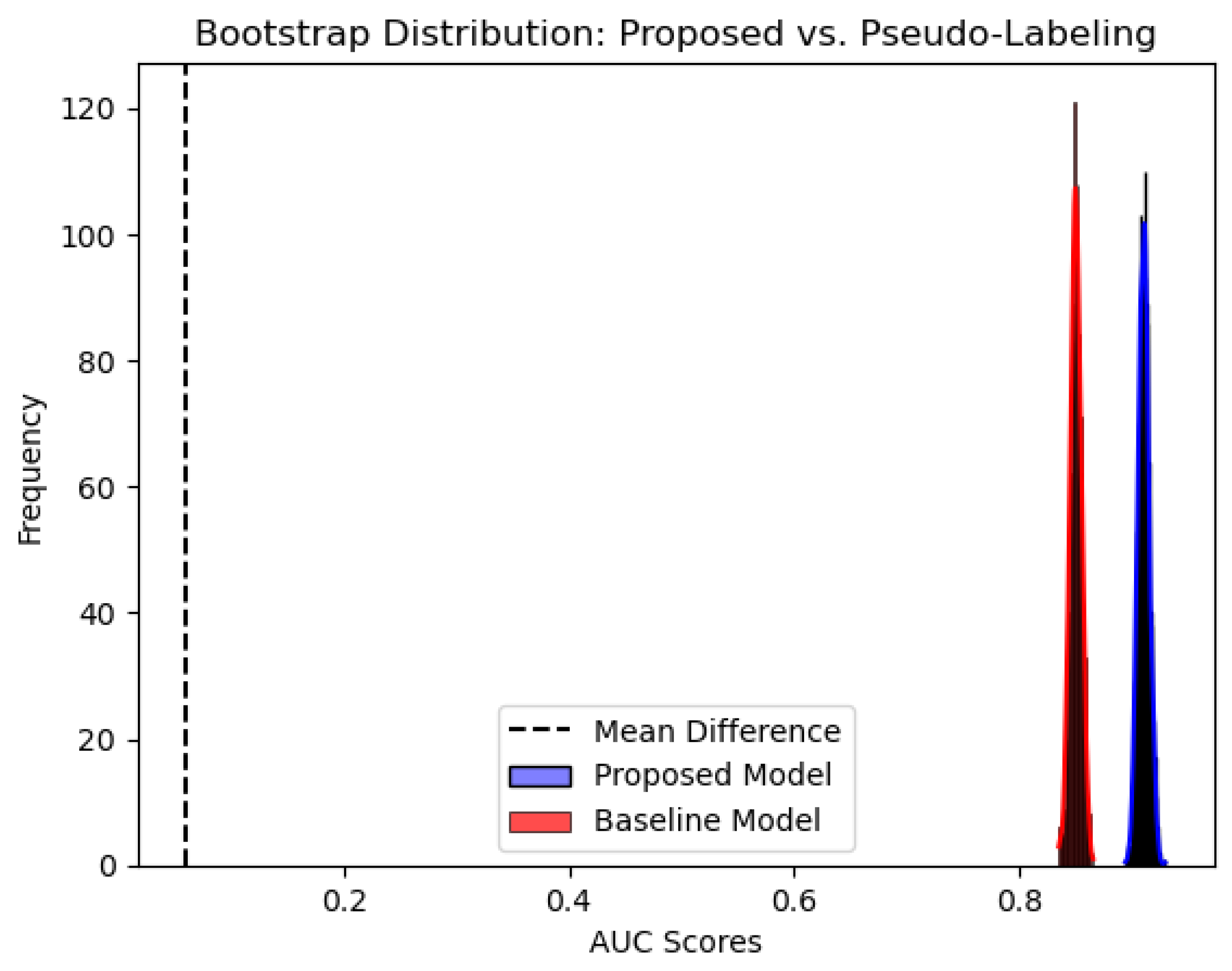
Figure 7.
Distribution of Conditional Entropy for 5% labeled Sparkify dataset. The majority of samples exhibit low entropy, indicating confident pseudo-labeling.
Figure 7.
Distribution of Conditional Entropy for 5% labeled Sparkify dataset. The majority of samples exhibit low entropy, indicating confident pseudo-labeling.
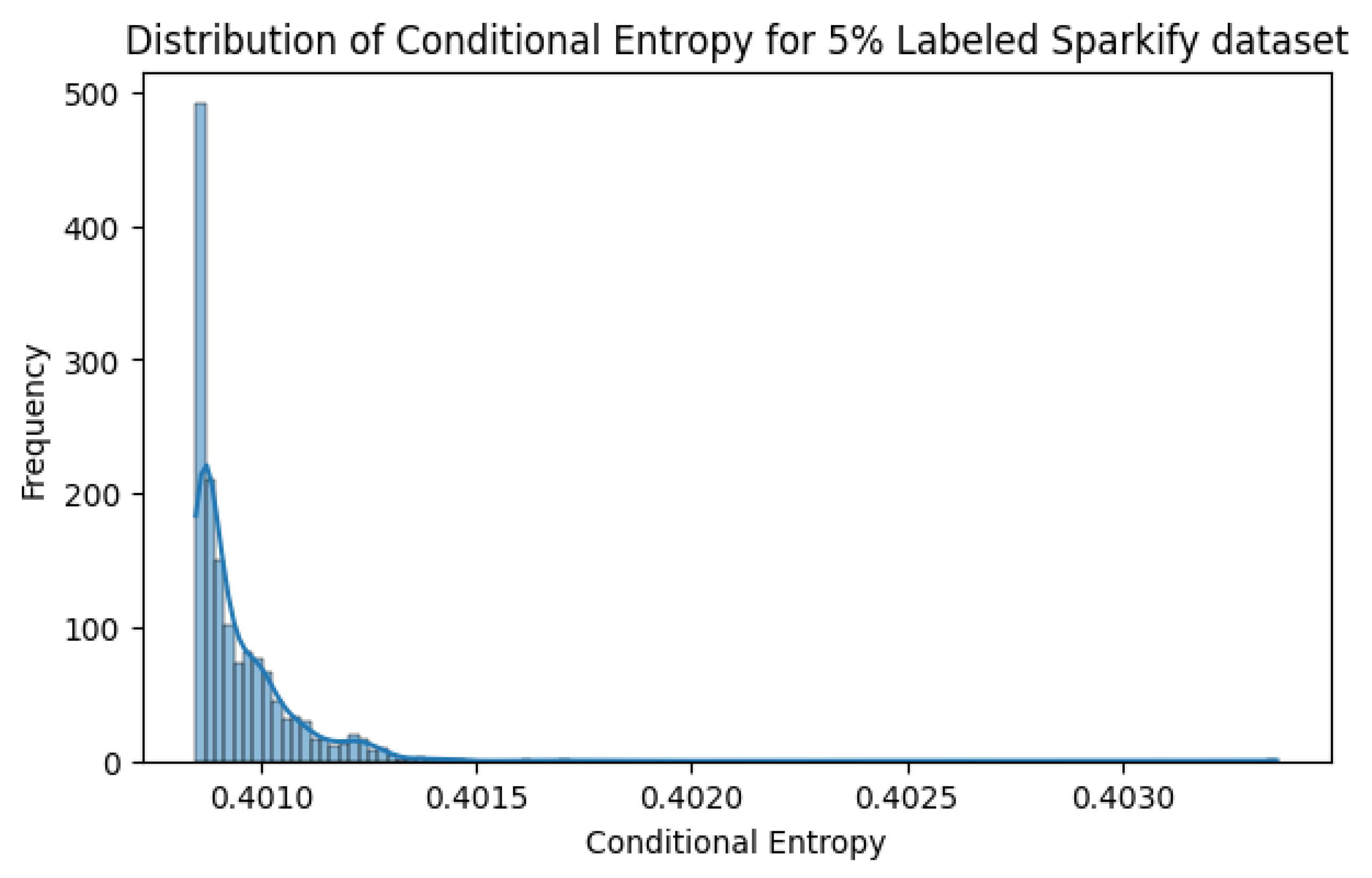
Figure 8.
Distribution of Conditional Entropy for 5% labeled IBM dataset. The majority of samples exhibit low entropy, indicating confident pseudo-labeling.
Figure 8.
Distribution of Conditional Entropy for 5% labeled IBM dataset. The majority of samples exhibit low entropy, indicating confident pseudo-labeling.
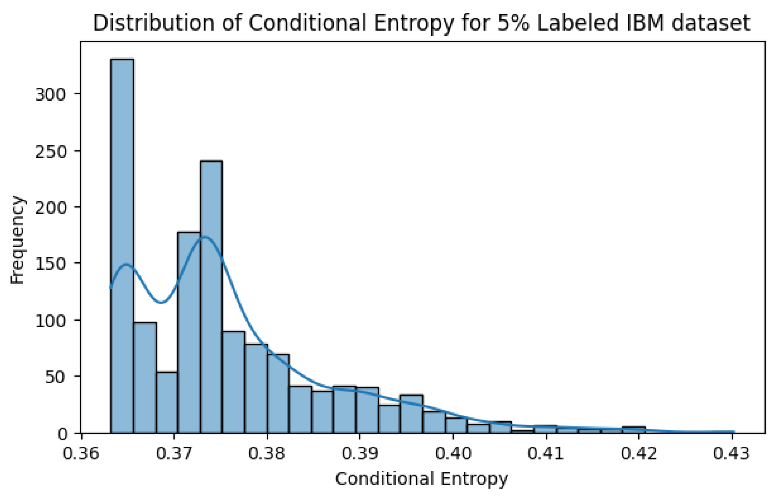
Figure 9.
ROC curve for the Sparkify dataset with 5% labeled data. The proposed model achieves an AUC of 0.91, demonstrating strong predictive performance.
Figure 9.
ROC curve for the Sparkify dataset with 5% labeled data. The proposed model achieves an AUC of 0.91, demonstrating strong predictive performance.
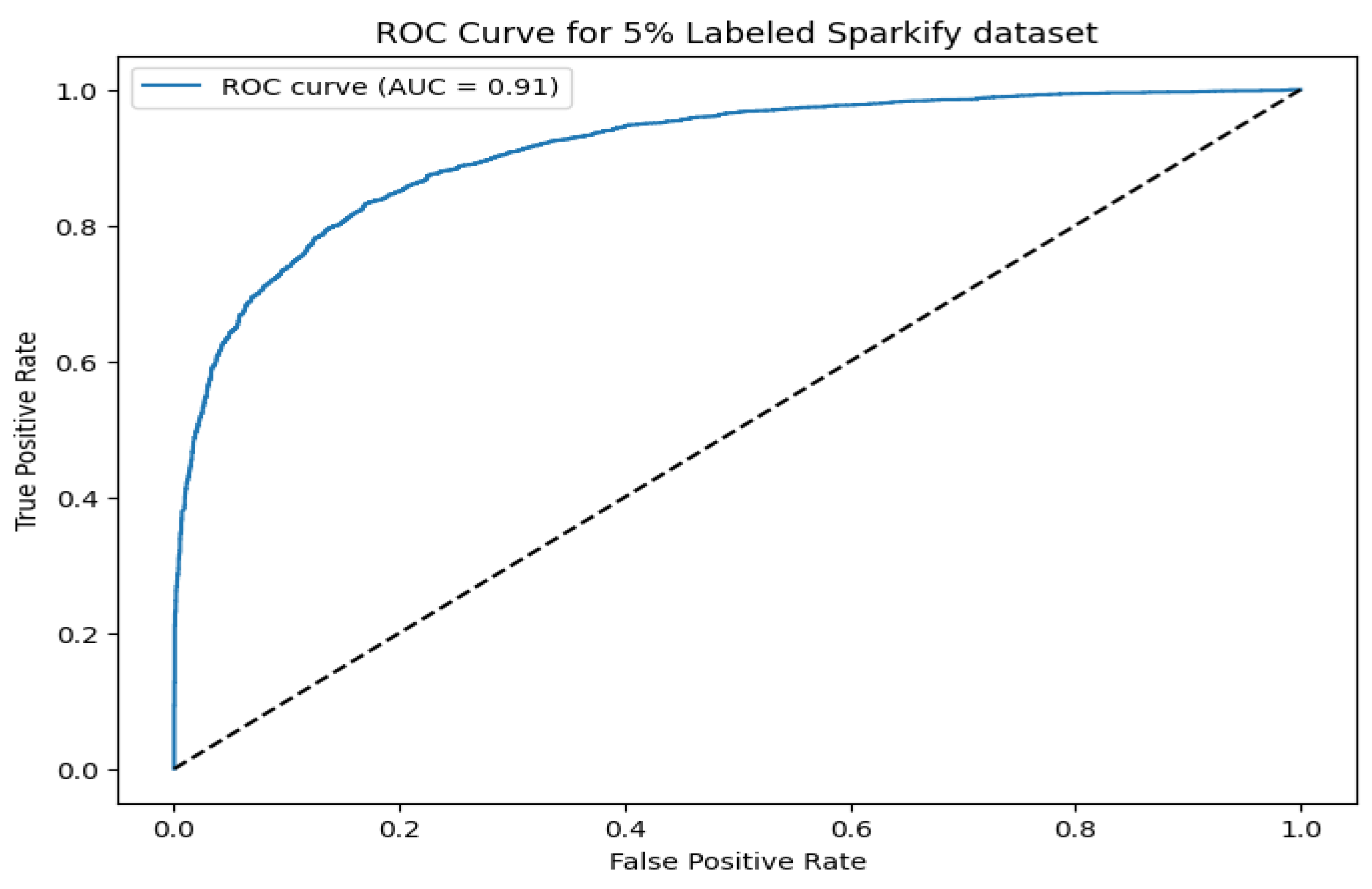
Figure 10.
ROC curve for the IBM dataset with 5% labeled data. The AUC of 0.89 highlights the model’s adaptability across datasets.
Figure 10.
ROC curve for the IBM dataset with 5% labeled data. The AUC of 0.89 highlights the model’s adaptability across datasets.
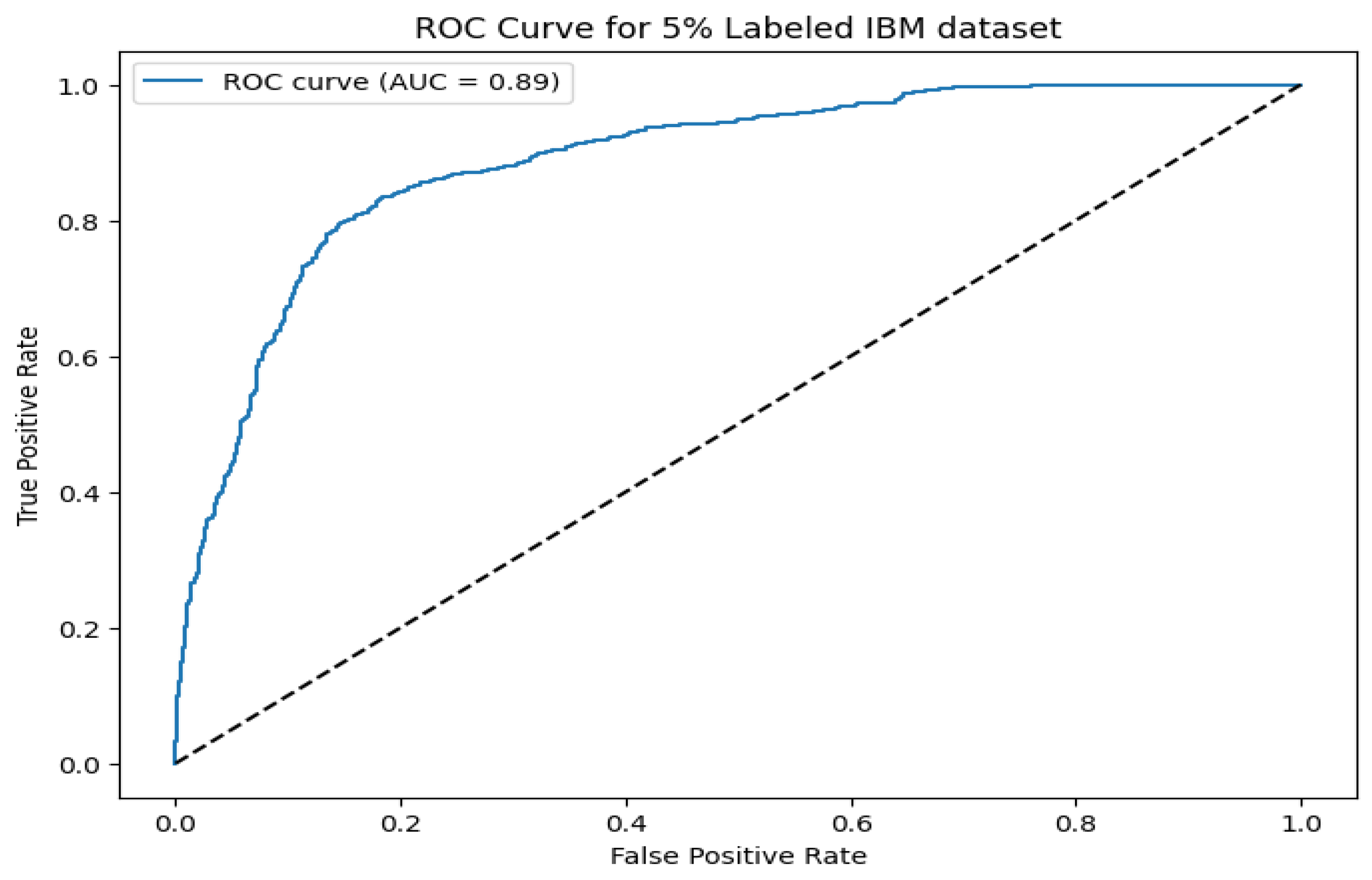
Figure 11.
Scalability analysis of the proposed model: Execution time (seconds) versus sample size, ranging from **50,000** to **300,000** samples. The blue line represents mean execution time, with the shaded area indicating ± standard deviation.
Figure 11.
Scalability analysis of the proposed model: Execution time (seconds) versus sample size, ranging from **50,000** to **300,000** samples. The blue line represents mean execution time, with the shaded area indicating ± standard deviation.
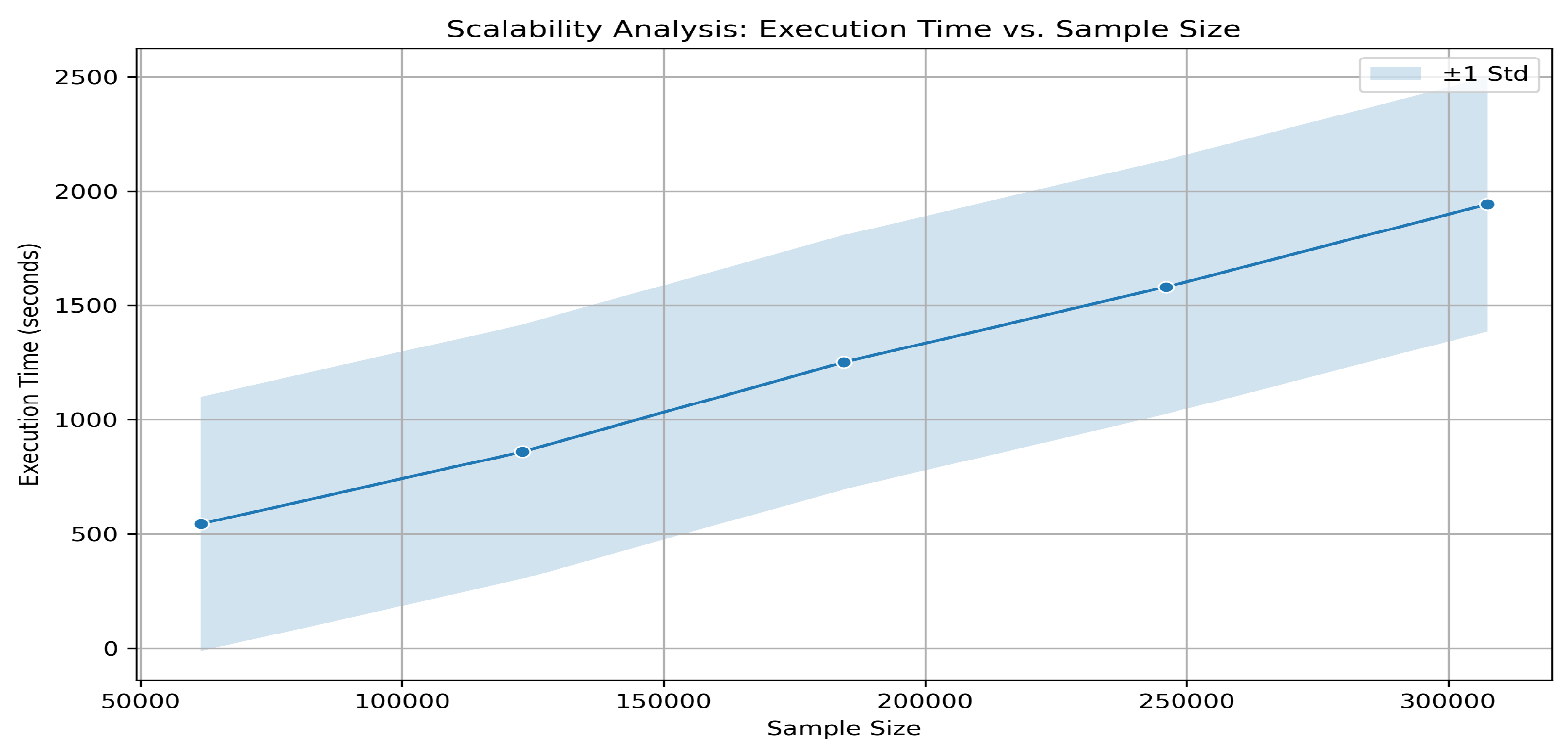

Table 1.
Comparison of Distance Metrics for Calibration.
| Metric | Key Strengths | Limitations |
|---|---|---|
| KL Divergence | Sensitive to distribution shape | Asymmetric; unstable with low probabilities |
| TV Distance | Bounded and straightforward | Ignores underlying data geometry |
| Hellinger Distance | Symmetric; robust to small changes | Limited in capturing spatial structure |
| Wasserstein Distance | Integrates magnitude and geometry | Higher computational cost (in >1D) |
Table 2.
Comparison of Calibration Methods.
| Method | Adaptivity | Robustness | Complexity |
|---|---|---|---|
| Static Temperature Scaling | No | Low | |
| Platt Scaling | No | Moderate | |
| Isotonic Regression | No | High (data-dependent) | |
| Proposed Adaptive Calibration | Yes | Very High |
Table 3.
Comparison of Diversity Sampling Methods.
| Method | Scalability | Diversity Guarantee | Additional Notes |
|---|---|---|---|
| Random Sampling | Low | No explicit diversity | |
| Clustering-Based Sampling (e.g., k-means) | Moderate | Sensitive to initialization | |
| DPP-based Sampling | High | Computationally prohibitive for large | |
| Proposed Multi-Resolution Hashing | (excl. SVD) | Competitive | Scales well with large datasets |
Table 4.
Comparison of Pseudo-Label Thresholding Methods.
| Method | Adaptivity | Robustness | Search/Optimization | Computational Cost |
|---|---|---|---|---|
| Fixed Threshold | No | Low | N/A | |
| Heuristic Tuning | Partial | Moderate | Manual/Ad hoc | |
| Grid Search | No | Moderate | Exhaustive Search | |
| Bayesian Optimization | Yes | High | Probabilistic Modeling | |
| Proposed Adaptive Method | Yes | Very High | Ternary Search over |
Table 5.
Dataset Overview and Selection Criteria.
| Dataset | Key Characteristics | Selection Rationale |
|---|---|---|
| Sparkify | Large-scale streaming logs (12.5GB, 26M records, 22K users) | Tests model scalability and temporal behavior modeling |
| IBM Telco | Structured telecom customer data (7,043 customers, 36 features) | Baseline comparison with demographic and service-based features |
| Bank Churn | Banking customer data (10K records, 14 financial features) | Evaluates financial churn prediction and high-cardinality categorical data |
| CrowdAnalytix | High-dimensional service metrics | Assesses feature selection techniques on a large feature space |
Table 6.
Class Distribution Before and After SMOTE.
| Dataset | Original | Balanced | ||
|---|---|---|---|---|
| Non-Churn | Churn | Non-Churn | Churn | |
| Sparkify | 17,274 | 5,003 | 17,274 | 17,274 |
| IBM Telco | 5,174 | 1,869 | 5,174 | 5,174 |
| Bank Churn | 7,963 | 2,037 | 7,963 | 7,963 |
| CrowdAnalytix | 36,336 | 14,711 | 36,336 | 36,336 |
Table 7.
Performance Comparison of Semi-Supervised Models (5% Labeled Data).
| Dataset | Model | AUC | F1 | TPR | FPR |
|---|---|---|---|---|---|
| Sparkify | Proposed Model | 0.9107 | 0.8296 | 0.8643 | 0.2177 |
| Pseudo-Labeling | 0.8501 | 0.8569 | 0.8138 | 0.1001 | |
| Tri-Training | 0.8518 | 0.8576 | 0.8210 | 0.1058 | |
| Label Spreading | 0.7037 | 0.7198 | 0.6676 | 0.2281 | |
| Uncertainty Sampling | 0.9036 | 0.8299 | 0.8068 | 0.1336 | |
| Query-by-Committee | 0.8995 | 0.8194 | 0.7868 | 0.1326 | |
| Diversity Sampling | 0.8946 | 0.8018 | 0.7458 | 0.1136 | |
| Core Set Selection | 0.9022 | 0.8160 | 0.7754 | 0.1243 | |
| BAAL | 0.9106 | 0.8399 | 0.8068 | 0.1136 | |
| Self-Training | 0.8447 | 0.7470 | 0.7127 | 0.1941 | |
| MixMatch | 0.8403 | 0.7330 | 0.6633 | 0.1453 | |
| Mean Teacher | 0.8427 | 0.7470 | 0.6984 | 0.1701 | |
| CoMatch | 0.8174 | 0.7219 | 0.6915 | 0.2226 | |
| IBM Telco | Proposed Model | 0.8902 | 0.8282 | 0.8389 | 0.1899 |
| Pseudo-Labeling | 0.8413 | 0.8294 | 0.8945 | 0.2356 | |
| Tri-Training | 0.8434 | 0.8314 | 0.8984 | 0.2356 | |
| Label Spreading | 0.7909 | 0.7588 | 0.9012 | 0.3836 | |
| Uncertainty Sampling | 0.9333 | 0.8532 | 0.8495 | 0.1937 | |
| Query-by-Committee | 0.9262 | 0.8516 | 0.8696 | 0.1823 | |
| Diversity Sampling | 0.9272 | 0.8543 | 0.8571 | 0.1748 | |
| Core Set Selection | 0.9355 | 0.8632 | 0.8830 | 0.1864 | |
| BAAL | 0.9275 | 0.8595 | 0.8504 | 0.1791 | |
| Self-Training | 0.8664 | 0.8068 | 0.7948 | 0.1876 | |
| MixMatch | 0.8249 | 0.7276 | 0.6836 | 0.2013 | |
| Mean Teacher | 0.6899 | 0.6469 | 0.6472 | 0.3621 | |
| CoMatch | 0.8893 | 0.7896 | 0.7287 | 0.2188 | |
| Banking | Proposed Model | 0.8417 | 0.7630 | 0.7907 | 0.2682 |
| Pseudo-Labeling | 0.7143 | 0.7211 | 0.7147 | 0.2715 | |
| Tri-Training | 0.7150 | 0.7220 | 0.7147 | 0.2707 | |
| Label Spreading | 0.6981 | 0.7025 | 0.7057 | 0.3007 | |
| Query-by-Committee | 0.8600 | 0.7725 | 0.8036 | 0.2671 | |
| Diversity Sampling | 0.8564 | 0.7873 | 0.8281 | 0.2686 | |
| Core Set Selection | 0.8557 | 0.7883 | 0.8152 | 0.2928 | |
| BAAL | 0.8572 | 0.7794 | 0.8088 | 0.2696 | |
| Self-Training | 0.8491 | 0.7756 | 0.8100 | 0.2819 | |
| MixMatch | 0.8416 | 0.7629 | 0.7906 | 0.2731 | |
| Mean Teacher | 0.8415 | 0.7628 | 0.7905 | 0.2793 | |
| CoMatch | 0.7431 | 0.6867 | 0.7366 | 0.3889 | |
| CrowdAnalytix | Proposed Model | 0.7065 | 0.6701 | 0.9781 | 0.9547 |
| Pseudo-Labeling | 0.6119 | 0.6912 | 0.4859 | 0.1035 | |
| Tri-Training | 0.6927 | 0.7254 | 0.6163 | 0.1655 | |
| Label Spreading | 0.5443 | 0.5627 | 0.5191 | 0.3937 | |
| Uncertainty Sampling | 0.7214 | 0.6447 | 0.5975 | 0.2597 | |
| Query-by-Committee | 0.7142 | 0.6378 | 0.5927 | 0.2695 | |
| Diversity Sampling | 0.7137 | 0.6355 | 0.5881 | 0.2664 | |
| Core Set Selection | 0.7160 | 0.6373 | 0.5945 | 0.2749 | |
| BAAL | 0.7214 | 0.6447 | 0.5975 | 0.2597 | |
| Self-Training | 0.6853 | 0.6111 | 0.5699 | 0.2995 | |
| MixMatch | 0.5763 | 0.5704 | 0.5848 | 0.4724 | |
| Mean Teacher | 0.5722 | 0.5382 | 0.5156 | 0.4063 | |
| CoMatch | 0.5769 | 0.5615 | 0.5707 | 0.4688 |
Table 8.
Performance Comparison of Semi-Supervised Models (10% Labeled Data).
| Dataset | Model | AUC | F1 | TPR | FPR |
|---|---|---|---|---|---|
| Sparkify | Proposed Model | 0.9326 | 0.8650 | 0.8472 | 0.1107 |
| Pseudo-Labeling | 0.8633 | 0.8697 | 0.8245 | 0.0851 | |
| Tri-Training | 0.8634 | 0.8676 | 0.8393 | 0.1041 | |
| Label Spreading | 0.7371 | 0.7456 | 0.7156 | 0.2243 | |
| Uncertainty Sampling | 0.9236 | 0.8487 | 0.8178 | 0.1087 | |
| Query-by-Committee | 0.9180 | 0.8372 | 0.8065 | 0.1194 | |
| Diversity Sampling | 0.9179 | 0.8349 | 0.7960 | 0.1101 | |
| Core Set Selection | 0.9188 | 0.8390 | 0.8094 | 0.1191 | |
| BAAL | 0.9236 | 0.8487 | 0.8178 | 0.1087 | |
| Self-Training | 0.8833 | 0.7825 | 0.7467 | 0.1606 | |
| MixMatch | 0.8526 | 0.7631 | 0.7382 | 0.1952 | |
| Mean Teacher | 0.8514 | 0.7687 | 0.7801 | 0.2477 | |
| CoMatch | 0.8071 | 0.7284 | 0.7281 | 0.2690 | |
| IBM Telco | Proposed Model | 0.9232 | 0.8445 | 0.8667 | 0.1889 |
| Pseudo-Labeling | 0.8445 | 0.8349 | 0.8366 | 0.2181 | |
| Tri-Training | 0.8441 | 0.8359 | 0.8210 | 0.2084 | |
| Label Spreading | 0.8046 | 0.7843 | 0.8600 | 0.3096 | |
| Uncertainty Sampling | 0.9384 | 0.8401 | 0.8582 | 0.1890 | |
| Query-by-Committee | 0.9381 | 0.8344 | 0.8155 | 0.1801 | |
| Diversity Sampling | 0.9335 | 0.8378 | 0.8541 | 0.1990 | |
| Core Set Selection | 0.9364 | 0.8320 | 0.8619 | 0.1894 | |
| BAAL | 0.9396 | 0.8299 | 0.8793 | 0.2098 | |
| Self-Training | 0.9266 | 0.8629 | 0.8593 | 0.2195 | |
| MixMatch | 0.9255 | 0.8427 | 0.8217 | 0.1996 | |
| Mean Teacher | 0.9328 | 0.8444 | 0.8266 | 0.2217 | |
| CoMatch | 0.8946 | 0.8054 | 0.7661 | 0.1383 | |
| Banking | Proposed Model | 0.8998 | 0.8185 | 0.8332 | 0.1929 |
| Pseudo-Labeling | 0.7793 | 0.7846 | 0.7798 | 0.2107 | |
| Tri-Training | 0.7790 | 0.7845 | 0.7785 | 0.2094 | |
| Label Spreading | 0.7626 | 0.7674 | 0.7663 | 0.2315 | |
| Uncertainty Sampling | 0.8572 | 0.7794 | 0.8088 | 0.2535 | |
| Query-by-Committee | 0.8600 | 0.7725 | 0.8036 | 0.2633 | |
| Diversity Sampling | 0.8564 | 0.7873 | 0.8281 | 0.2621 | |
| Core Set Selection | 0.8557 | 0.7883 | 0.8152 | 0.2407 | |
| BAAL | 0.8572 | 0.7794 | 0.8088 | 0.2535 | |
| Self-Training | 0.8491 | 0.7756 | 0.8100 | 0.2652 | |
| MixMatch | 0.8925 | 0.8072 | 0.8545 | 0.2498 | |
| Mean Teacher | 0.8864 | 0.8010 | 0.8487 | 0.2572 | |
| CoMatch | 0.7361 | 0.6823 | 0.7592 | 0.4434 | |
| CrowdAnalytix | Proposed Model | 0.7948 | 0.7137 | 0.5801 | 0.0463 |
| Pseudo-Labeling | 0.5283 | 0.6570 | 0.3835 | 0.0690 | |
| Tri-Training | 0.6811 | 0.7324 | 0.5700 | 0.1052 | |
| Label Spreading | 0.5637 | 0.5773 | 0.5426 | 0.3880 | |
| Uncertainty Sampling | 0.7348 | 0.6591 | 0.6117 | 0.2481 | |
| Query-by-Committee | 0.7307 | 0.6546 | 0.6099 | 0.2571 | |
| Diversity Sampling | 0.7261 | 0.6488 | 0.6019 | 0.2569 | |
| Core Set Selection | 0.7322 | 0.6578 | 0.6180 | 0.2646 | |
| BAAL | 0.7348 | 0.6591 | 0.6117 | 0.2481 | |
| Self-Training | 0.7117 | 0.6170 | 0.5437 | 0.2216 | |
| MixMatch | 0.5955 | 0.5509 | 0.5215 | 0.3771 | |
| Mean Teacher | 0.6022 | 0.5720 | 0.5621 | 0.4090 | |
| CoMatch | 0.5772 | 0.5409 | 0.5258 | 0.4241 |
Table 9.
Proposed Model Execution Time (in seconds).
| Dataset | 5% Labeled Data | 10% Labeled Data |
|---|---|---|
| Sparkify Churn Dataset | 89.39 | 82.67 |
| IBM Telecom Churn Dataset | 78.24 | 19.73 |
| Bank Churn Dataset | 11.84 | 27.17 |
| CrowdAnalytix Telecom Churn Dataset | 220.41 | 79.30 |
Table 10.
Robustness Analysis with Label Noise on Sparkify Dataset.
| Noise Level | F1 Score | AUC | TPR | FPR |
|---|---|---|---|---|
| 0% | 0.8469 | 0.9192 | 0.8170 | 0.1116 |
| 5% | 0.8333 | 0.9089 | 0.8164 | 0.1419 |
| 10% | 0.7912 | 0.8874 | 0.7237 | 0.1050 |
| 15% | 0.7911 | 0.8809 | 0.7382 | 0.1272 |
Table 11.
Ablation Study Results on Sparkify (5% Labeled Data).
| Variant | Final AUC | Final F1 | Final TPR | Final FPR | Execution Time (s) |
|---|---|---|---|---|---|
| Proposed Model | 0.9107 | 0.8296 | 0.8643 | 0.2177 | 89.39 |
| No WCE | 0.5322 | 0.6650 | 1.0000 | 0.4981 | 128.41 |
| No ATO | 0.5339 | 0.5517 | 0.5997 | 0.5108 | 101.97 |
| No Diversity | 0.5522 | 0.6649 | 0.9997 | 0.4981 | 123.43 |
Table 12.
Ablation Study Results on Sparkify (10% Labeled Data).
| Variant | Final AUC | Final F1 | Final TPR | Final FPR | Execution Time (s) |
|---|---|---|---|---|---|
| Proposed Model | 0.9326 | 0.8650 | 0.8472 | 0.1107 | 82.67 |
| No WCE | 0.4632 | 0.6646 | 0.9988 | 0.4980 | 82.45 |
| No ATO | 0.5007 | 0.4719 | 0.4372 | 0.5124 | 70.34 |
| No Diversity | 0.4711 | 0.6643 | 0.9983 | 0.4978 | 80.24 |
Table 13.
Summary of Statistical Test Results. The Wilcoxon signed-rank test statistic and p-values are provided along with the bootstrapped mean AUC difference and Cohen’s d effect size. Tests are based on 10+ paired observations per comparison across multiple seeds and labeling scenarios.
Table 13.
Summary of Statistical Test Results. The Wilcoxon signed-rank test statistic and p-values are provided along with the bootstrapped mean AUC difference and Cohen’s d effect size. Tests are based on 10+ paired observations per comparison across multiple seeds and labeling scenarios.
| Comparison | Wilcoxon Signed-Rank | Bootstrapped AUC Difference | Cohen’s d |
|---|---|---|---|
| Proposed vs. Pseudo-Labeling | (0.0000, 0.0000) | 0.0604 [0.0599, 0.0608] | 12.2104 |
| Proposed vs. BAAL | (245398.0000, 0.5953) | 0.0002 [-0.0002, 0.0006] | 0.0341 |
| Proposed vs. Core Set | (20555.0000, 0.0000) | 0.0087 [0.0083, 0.0091] | 1.7321 |
| Proposed vs. CoMatch | (0.0000, 0.0000) | 0.0937 [0.0932, 0.0941] | 18.9980 |
Table 14.
Performance Comparison on Home Credit Dataset (10% Labeled Data).
| Model | AUC | F1 | TPR | FPR |
|---|---|---|---|---|
| FreeMatch | 0.5703 ± 0.0029 | 0.0506 ± 0.0439 | 0.0359 ± 0.0322 | 0.0212 ± 0.0191 |
| Proposed | 0.5566 ± 0.0199 | 0.1291 ± 0.0225 | 0.4521 ± 0.2941 | 0.2117 ± 0.1116 |
Table 15.
Sensitivity Analysis Results for FreeMatch.
| Seed | F1 | AUC | TPR | FPR |
|---|---|---|---|---|
| 42 | 0.0435 ± 0.0018 | 0.5571 ± 0.0027 | 0.0266 ± 0.0012 | 0.0172 ± 0.0002 |
| 123 | 0.0284 ± 0.0034 | 0.5542 ± 0.0015 | 0.0162 ± 0.0020 | 0.0106 ± 0.0002 |
| 456 | 0.0005 ± 0.0004 | 0.5418 ± 0.0038 | 0.0002 ± 0.0002 | 0.0002 ± 0.0000 |
Table 16.
Sensitivity Analysis Results for Proposed Model.
| Seed | F1 | AUC | TPR | FPR |
|---|---|---|---|---|
| 42 | 0.1023 ± 0.0011 | 0.5347 ± 0.0009 | 0.1063 ± 0.0013 | 0.0850 ± 0.0004 |
| 123 | 0.1450 ± 0.0000 | 0.5600 ± 0.0008 | 0.6500 ± 0.0000 | 0.3000 ± 0.0000 |
| 456 | 0.1400 ± 0.0000 | 0.5550 ± 0.0016 | 0.6000 ± 0.0000 | 0.2500 ± 0.0000 |
Disclaimer/Publisher’s Note: The statements, opinions and data contained in all publications are solely those of the individual author(s) and contributor(s) and not of MDPI and/or the editor(s). MDPI and/or the editor(s) disclaim responsibility for any injury to people or property resulting from any ideas, methods, instructions or products referred to in the content. |
© 2025 by the authors. Licensee MDPI, Basel, Switzerland. This article is an open access article distributed under the terms and conditions of the Creative Commons Attribution (CC BY) license (http://creativecommons.org/licenses/by/4.0/).
Copyright: This open access article is published under a Creative Commons CC BY 4.0 license, which permit the free download, distribution, and reuse, provided that the author and preprint are cited in any reuse.


