Submitted:
09 June 2025
Posted:
09 June 2025
You are already at the latest version
Abstract
Air pollution in urban areas has significantly increased over the last few years due to industrialization and overpopulation. Therefore, accurate predictions are needed to minimize their impact. This paper presents a neural network-based approach for Air Quality Index (AQI) forecasting, applying two different models: a variable depth neural network (NN) called slideNN, inspired by the capabilities of a Recurrent Neural Network (RNN) and a Gated Recurrent Unit (GRU)-based model. Both models use past particulate matter measurements alongside local meteorological data as inputs. Then, this research explores the practical application of multi-depth and recurrent neural networks in air quality forecasting, providing a hands-on case study and model evaluation for the city of Ioannina, Greece, targeting the appliance of such models either on edge devices or as cloud services. SlideNN variable-depth architecture consists of multiple independent neural sub-model strands varying in size, enhancing feature extraction and predictive accuracy. At the same time, the GRU model is examined on its ability to capture temporal dependencies in the data. Finally, both models are combined to offer a cloud-based high-precision hybrid. Experimental results show that the GRU model consistently outperforms the variable-depth architecture regarding forecasting losses. In contrast, complex hybrid GRU-NN models outperform both, delivering additional localized information that can be exploited by established particle concentration map monitoring services.
Keywords:
air quality index
; air pollution
; neural networks
; deep learning
; forecasting
; recurrent neural network
; edge computing
; cloud computing
1. Introduction
Air pollution remains a serious global environmental and public health safety challenge of the 21st century. Recent studies indicate that 99% of the world’s population is exposed to particulate matter (PM) concentrations exceeding World Health Organization (WHO) safety limits, with ambient (outdoor) and household pollution collectively contributing to 6.7 million premature deaths annually through cardiovascular, respiratory, and oncological issues [1,2,3]. The economic burden is equally severe, with global welfare losses estimated at $8.1 trillion (6.1% of GDP), driven by healthcare expenditures and productivity declines [4].
The Air Quality Index (AQI) is a standardized metric used globally to communicate how polluted the air is or is about to become. It translates complex air quality data into a single number and color code ranging from 0 (good) to 500 (hazardous), making it easier for the public to contemplate the health risks associated with pollutants such as PM2.5, PM10, O3 and NO2 [5]. Table 1 below shows that AQI categories directly correlate with population health risks, guiding public advisories, and policy interventions during pollution episodes [6].
Regarding AQI monitoring, IQAir is a leading company in air quality monitoring. It offers IoT devices and services that track quality. Their range of outdoor sensors enables monitoring of pollutants like PM10, PM2.5, , temperature, and humidity. These sensors also integrate with the IQAir Map platform, a real-time interactive map that visualizes air pollution levels, as well as an appropriate mobile phone application [7]. Similarly Clarity Node-S, is an industrial graded solar-powered, and cellular-connected IoT sensor that measures key pollutants such as PM2.5, , and ozone in real time [8].
In Greece, urban centers like Athens, Thessaloniki, and Ioannina face persistent air quality challenges, with winter PM2.5 and PM10 levels often exceeding WHO guidelines by 300–400% due to vehicular emissions, house heating, and trans-boundary pollution [9,10,11,12,13,14]. For instance, Ioannina’s annual PM2.5 average of in 2023 surpassed the WHO annual guideline () by 300% [15] and the EU limit value by 100% [16], reflecting cooperative impacts from local biomass-wood combustion (contributing 60–70% of winter PM2.5) and long-range Saharan dust transport [14,17,18].
Accurate air quality predictions are a necessity nowadays. That is why many scientists focused on and made notable progress on this matter, which is due to the significance of the remaining and upholding challenges. A critical limitation stems from incomplete data dimensionality in most existing models. Traditional approaches frequently treat meteorological parameters (e.g., temperature, humidity, wind patterns) and particulate matter concentrations (PM1, PM2.5, PM10) as independent variables, failing to capture their complex synergistic interactions [19]. This simplification neglects their intricate relationship, particularly during pollution events. As it has been indicated by Wang et al. [20], humidity-driven PM2.5 hygroscopic growth exhibits strong nonlinear relationships that substantially impact prediction accuracy when ignored. Models failing to account for these interactions show significantly higher errors during high-humidity conditions.
The predominance of short-term forecasting approaches presents additional challenges. Although short-term forecasts typically yield lower prediction errors, long-term PM2.5 forecasting is essential for adequate public health protection and air quality management. It is important to mention that during winter, biomass burning causes pollution levels to rise sharply and unpredictably due to domestic heating activities [21]. Furthermore, meteorological variability, particularly temperature, and wind speed can significantly impact particulate matter concentrations, increasing uncertainty in predictiviness of the deep learning models [22].
Moreover, in recent years, several models based on Bi-directional Long Short-Term Memory(Bi-LSTM) architectures have been proposed for air quality prediction due to their ability to capture temporal dependencies for both past and future data tendencies. While, in theory, this type of model shows promise, in practice, it has revealed some crucial flaws [23,24,25]. For instance, in a comparative study of PM2.5 prediction models across Seoul, Daejeon, and Busan [26], Bi-LSTM models demonstrated high accuracy for short-term forecasts (within 24 hours). However, they showed a significant drop in performance for longer-term predictions, with values decreasing to 0.6, indicating challenges in maintaining accuracy over extended periods. Furthermore, the computational complexity of Bi-LSTM models can make them less convenient and practical for real-time applications as it can lead to increased training times and resource consumption [27].
To address these challenges, this study introduces a framework that acknowledges the correlation between the particulate matter and meteorological data and shows long-term accurate forecasting results consisting of two distinct architectures to do so:
- A sliding-window feedforward model (slideNN) includes four neural sub-models of varying sizes, each designed to process different input lengths efficiently and offer short-term accuracy and efficient training performance.
Compared to other already existing deep learning(DL) solutions, both models -each one for a distinct use- show significant improvements in predictive accuracy, generalization, and robustness to noise. These refinements are especially evident in industrial urban regions, where air quality patterns are highly nonlinear and affected by multiple environmental factors.
This paper is organised as follows: Section 2 presents the proposed AQI forecating framework using particulate matter and meteorological data and its correspoding slideNN and variable length GRU models. Section 3 presents the authors’ experimental scenarios evaluating the framework models, and Section 4 concludes the paper.
2. Materials and Methods
In order to utilize local weather conditions information along with particle matter concentration measurements to classify and forecast air quality via AQI predictions, the authors propose a new framework that takes as input a combination of past meteorological measurements along with particle concentrations. Following a susceptible transformation, this data augmentation can be used as input into different types of deep learning models. Two types of models are examined as part of the framework, taking into account the time series depth: 1) A composite-stranded NN model and 2) a variable-length GRU Recurrent Neural Network. Both model categories are further classified into edge computing and cloud computing models based on the number of parameters they pertain.
Meteorological measurements that are used as normalized inputs by the framework’s models are local measurements of temperature, humidity, and wind speed direction vectors, while for particle concentrations PM1, PM2.5, PM4, and PM10 particulate matter concentrations measured in g/m3. PM4,10 measurements track coarse pollution from dust and industrial emissions, while PM1-2.5 track more dangerous materials related to heart and lung diseases. Furthermore, temperature, humidity, and wind measurements try to encode how these conditions affect the dispersion of particulate matter (PM) in the atmosphere or to predict PM concentrations under specific localized meteorological conditions. In conclusion, the proposed model uses vector data of combined and normalized meteorological and particulate matter measurements as inputs and tries either to classify or forecast current or future AQI index values.
2.1. Proposed Framework for AQI Forecasting
The proposed framework consists of two distinct modeling approaches for air quality forecasting. The first is a Neural Network (NN) model composed of multiple sub-models, called strands as a unified structure, each strand of varying input size [30,31]. This design enables adaptability to different input lengths while preserving structural coherence. The input for the NN model is a time series of particulate and meteorological measurements formatted as a one-dimensional (1D) matrix with all data points sequentially arranged. Its output consists of predicted AQI values for specific future hours, depending on the selected sub-model, ensuring scalability across various temporal resolutions. To this extent, a second model based on Gated Recurrent Units (GRUs) is developed to enhance predictive performance. The GRU model utilizes temporal dependencies within the time series more effectively, improving forecasting accuracy over extended periods. These models provide a robust framework for flexible real-time deployment on edge devices and high-accuracy air quality prediction. The proposed models were constructed using the Tensorflow Keras framework [32,33].
2.2. Proposed Deep-Learning Models
In addition to the architectural differences between the models mentioned in the previous Section 2.1, the authors adopted two distinct approaches regarding data processing and storage, distinguishing between edge and cloud computing implementations. Their indicative design is as follows:
-
One perspective focuses on the implementation of both the neural network and the previously mentioned GRU model within an edge computing framework. In this scenario, both models are designed to receive identical timesteps and data parameters to ensure comparable model sizes, which are intentionally kept smaller to meet the constraints and computational limitations of edge devices. Notably, edge computing is increasingly adopted in air quality monitoring applications, as it enables efficient, low-latency forecasting in resource-constrained environments [34,35]. Such integration of AI at the edge is especially beneficial for real-time, autonomous air pollution assessment [36].Furthermore, these models could be integrated into micro-IoT devices or even embedded directly into environmental sensors [37]. Based on their localized measurements — which align with the features used during model training — the models would be capable of generating short-term forecasts of Air Quality Index (AQI) values. This approach is particularly suitable for short term prediction horizons, where timely and on-site decision making is critical.
-
The second approach focuses on large-scale air quality forecasting through cloud computing. In this case, only the GRU-based model is used, with a significantly larger number of GRU cells and layers, in an effort to fully utilize the computational resources and scalability offered by cloud infrastructure.Unlike edge-based implementations, cloud computing is not constrained by memory or processing limitations, enabling the use of deeper architectures and more complex temporal dependencies. This makes it particularly suitable for long-term predictions and the collection of data from multiple sources, such as distributed sensor networks or satellite feeds [38,39]. Recent studies have demonstrated the efficiency of cloud-based systems in air quality monitoring. For instance, the integration of wireless sensor networks with cloud computing has been shown to facilitate real-time data collection and analysis, enhancing the responsiveness and accuracy of air quality assessments [40].The model can be trained and deployed using higher dimensional input vectors thanks to the cloud’s virtually unlimited computing capacity, which allows it to pick up more subtle patterns in variations in air quality over time. Because of this, it works especially well for regional forecasting, policy assessment, and assisting with large-scale environmental monitoring systems.
Figure 1 depicts the entire data processing and model deployment workflow implemented in this study. The process starts with raw input data, which goes through validation and temporal preprocessing before being used to train the proposed neural network models. Depending on the forecasting scale, computational requirements, and user-specific restrictions, the most appropriate model architecture is chosen, followed by a deployment strategy targeting either edge computing environments or cloud-based platforms. This workflow ensures flexibility, scalability, and maximum usage of the given resources . Each step of the process, from data preparation and model training to performance evaluation and final deployment, is discussed in detail in the Section 2.2.1 and Section 2.2.2.
2.2.1. SlideNN Model
The neural network architecture, called the slideNN model, follows a specific recursive relationship that governs the structure of all four sub-model strands, defining the input size, the number of neurons per layer, and the output size similar to [31]. However, the recursive pattern in slideNN indicates a systematic "leftward shift" in these parameters as we progress through the models. Specifically, each model has an input layer of size , where depending on the sub-model, and at each subsequent hidden layer, the number of neurons decreases following a power-of-two pattern. This reduction continues until the output layer contains neurons, where .
The recursive relationship ruling the neural network models is defined as follows: Let denote the input layer size, where for some integer k. The number of neurons at each hidden layer follows the recurrence relation, given by Equation 1.
where d is the network depth such that , representing the output layer size.
For a given model , the relationship is expressed as:
where denotes the model index, corresponding to input sizes respectively.This formulation captures the systematic leftward shift of input size, hidden layers, and output size as we transition from one model to the next. The layer architecture and configuration of each submodel are also shown in Figure 2.
2.2.2. Variable Length-GRU Model
In contrast to the stranded-partitioned architecture of the NN edge device model, the GRU-based model makes better use of the temporal modeling capabilities of recurrent neural networks. This model is structured to handle sequential data with a fixed number of timesteps and feature attributes, specifically tailored for AQI forecasting using both meteorological and particulate matter measurements, with inputs formatted as one-dimensional vectors of length t, where t denotes the number of timesteps. Before entering the GRU layers, each input vector is reshaped into a three-dimensional tensor of shape, where n is the number of samples, k is the number of feature attributes and represents the sequence length. The model’s core consists of n stacked GRU layers containing m units. All but the final GRU layer returns full sequences to preserve temporal context across layers. The final GRU layer outputs a fixed-length vector representation of the input sequence, which is passed through a series of fully connected layers.
Depending on the value of m, the dense block behaves accordingly :
- For smaller values of , a single dense layer with m neurons is applied.
- For larger values of , the dense block consists of a sequence of layers starting from m, halving in size each time until reaching 64, allowing for a gradual dimensionality reduction.
The final output layer consists of ℓ neurons corresponding to the number of AQI values predicted. The number of output neurons ℓ is not chosen arbitrarily but is derived as a function of the input sequence length t. Specifically, it follows the relation shown in Equation 2:
Formally, let represent a single flattened input sequence. The transformation applied by the model is summarized in Equation 3.
where is the reshaped input, h is the output of the final GRU layer, z is the output of the dense block, and is the final output vector of predicted AQI values. The architecture allows for flexible hyperparameter tuning in terms of the number of GRU layers (n), the size of each layer (m), the timestep length (t), and the number of output values (ℓ).
Different architectural results and GRU layer configurations were implemented depending on whether the model was intended for edge or cloud computing environments. These architectural designs are illustrated in Figure 3 and [2], corresponding to the edge and cloud settings, respectively.
In the edge-case GRU, each configuration consistently featured two hidden GRU layers, with the number of GRU cells varying among 16, 32, 64, and 128, depending on the input size. For configurations where the number of GRU cells reached above 128 (which did not occur in the edge case but is architecturally accounted for), the subsequent dense layers were reduced by a power of two at each step until reaching 128 cells, promoting efficient computation and compactness suitable for constrained environments.
In contrast, the cloud-based GRU models adopted a deeper architecture with four internal layers, and were characterized by significantly larger GRU sizes. The GRU layers in this case started at 1280 cells, and decreased progressively by powers of two through the following sizes: , eventually stopping once the size dropped below 64. This structure reflects the cloud setting’s capacity to support more complex and memory-intensive models, offering a broader and more expressive architecture for improved learning capacity.
Table 2 includes the hyperparameters of each model separately used in this study:
2.3. Data Collection and Preprocessing
Before delving into the specific datasets, it is important to note that the data used in this study was collected from multiple sources located in Ioannina, Greece, spanning the period from January 2021 to December 2023. The primary air quality measurements originate from IoT-based particulate matter (PM) sensors installed in central urban locations of the city, specifically in the area of Vilaras Street near the Zosimaia School. These sensors provide continuous hourly data for four types of particulate matter: PM1, PM2.5, PM4, and PM10. Complementary meteorological data—including temperature (T), relative humidity (H), wind speed (WS), and wind direction (WD)—were recorded by the official meteorological station of the University of Ioannina [41]. Each hourly entry in the dataset forms an 8-dimensional feature vector: (PM1, PM2.5, PM4, PM10, T, H, WS, WD), where PMs are the particle matter concentrations (1–10) and T,H,WS, and WD are the meteorological station measurements of temperature, relative humidity, wind speed, and direction accordingly.
Over a monitoring period of the three-year period, the dataset comprises more than 26,000 complete hourly measurements, providing a high temporal resolution essential for short and medium-term air quality forecasting. The dataset underwent a series of preprocessing steps to ensure consistency and model preparation. These included handling missing values and applying feature-wise normalization and standardization techniques to account for unit and value range disparities across the input variables, as well as data partitioning at the minute level using linear interpolation ( total measurements).
2.3.1. Data Preprocessing
The primary pollutant indicators used in this study are particulate matter (PM) concentrations, separated into 4 distinct types based on their size: PM1, PM2.5, PM4, PM10. These pollutants are significant contributors to air quality degradation, originating from various natural and anthropogenic sources, such as industrial emissions, vehicle exhaust, and biomass burning [42,43]. The dataset consists of time-series measurements of these particulate concentrations, recorded in micrograms per cubic meter ().
Particulate matter features were subjected solely to standardization using z-score normalization. This method transforms each input variable such that it has a mean of zero and a standard deviation of one, effectively centering and scaling the data:
Here, is the mean and is the standard deviation of each PM variable, computed using the training data. This transformation is particularly important for neural networks, as it ensures that features with larger numeric ranges do not dominate the training process. It also improves the conditioning of the optimization problem and speeds up convergence during training [44,45].
Meteorological Data: Meteorological variables are crucial for AQI forecasting as they influence pollutant dispersion, deposition, and transformation. This study incorporates temperature (°C), humidity (%), wind speed (m/s), and wind direction (°) [46].
For the meteorological variables, a two-stage preprocessing pipeline was implemented. The raw values of the meteorological variables were first standardized, using the same z-score formula as Equation 4. This was followed by Min-max normalization to scale the standardized values into a bounded range between 0 and 1 and shown in Equation 5:
This combined approach was chosen to accommodate both the need for zero-centered inputs and the benefits of scaled features within a uniform range [47]. Notably, min-max normalization was applied after standardization, using the minimum and maximum values of the standardized training data to ensure consistency and prevent information leakage.
The output dataset, consisting of future Air Quality Index (AQI) values, underwent a preprocessing strategy designed to accommodate the structure of the prediction models and improve training stability. Specifically, the number of future AQI values used as prediction targets varied depending on the model configuration. Four distinct input sizes of 64, 128, 256, and 512 hourly data points were selected. For each of these, the output consisted of the subsequent 2, 4, 8, and 16 hourly AQI values, respectively.
To construct the output dataset, specific rows were selected from the full AQI time series. More specifically for each input size, continually for every consecutive rows where , the following hourly AQI data where were chosen as prediction targets. This slicing strategy ensured temporal separation between training samples and helped prevent excessive overlap in prediction windows, thereby reducing potential data leakage and autocorrelation bias during training and evaluation [48].
For further clarity regarding the input and output configurations, Table 3 presents a summary of the respective settings used in the prediction process.
After the slicing process, the final output dataset that is used was created and all AQI target values were standardized using z-score normalization, according to Equation 6:
where and are the mean and standard deviation of the AQI values across the training targets.
Standardizing the output proved to be a crucial step in reducing prediction errors and stabilizing the training process [49]. Without standardization, the models exhibited significantly higher loss fluctuations and slower convergence, particularly when predicting multiple future time steps with higher variability in AQI levels.
After completing the data preprocessing phase, a final reshaping step was applied to convert the input data into a format compatible with the two different architectures individually. Initially, the input was structured as a sequence of rows, where each row corresponded to a single hourly observation and included the eight known variables.
2.3.2. Preprocessing for slideNN
Having to construct fixed-size input vectors, consecutive groups of rows were accumulated and flattened into one-dimensional(1D) arrays. Each model configuration defined a specific number of rows to be grouped based on the corresponding input size:
- The first model combined 8 consecutive rows () into a 64-element vector.
- The second model used 16 consecutive rows () resulting in 128-element vectors.
- The third model added 32 consecutive rows () turning them into 251-element vectors.
- The fourth model used 64 consecutive rows () and making 512-element vectors.
Mathematically, let be a matrix representing n consecutive hourly observations, each with 8 features. The reshaping process transforms this into a one-dimensional input vector as shown by Equation 7:
where is the feature of the hourly record. This operation preserves the temporal order of observations while converting them into a flat format suitable for fully connected feedforward neural networks. In Figure 5 each model’s reshaping process is depicted for a better understanding.
2.3.3. GRU Model Preprocessing
Although recurrent neural networks typically require 3D input shapes to capture temporal dynamics, in this implementation the GRU model receives the same flattened 1D input vectors as the feedforward slideNN model. Specifically, each input vector has a total temporal length (timestep) t, which results from flattening l timesteps with features each (coresponding to environmental conditions and particle matter concentrations), expressed bu Equation 8
where t is the total input size, is the number of features per timestep, flattened and set with a specific order over timesteps as an 1D vector, and l is the number of effective timesteps (e.g., 8, 16, 32, or 64). Before feeding the data into the GRU layers, an internal reshaping step is applied to convert each 1D vector of shape into a 2D matrix of shape , as follows:
This reshaping process aligns the input format with the GRU’s expected 3D tensor shape (including batch size):, where m is the number of input samples. Importantly, while the slideNN model uses the 1D input directly, the GRU model performs this additional transformation internally to reconstruct the temporal sequence from the same flattened vector. This design ensures structural compatibility while maintaining architectural consistency across both models.
2.4. Training Process and Metrics
The neural network models, as well as the GRU models, were trained using the Root Mean Squared Error (RMSE) as the loss function, which is well-suited for regression tasks and has been used as the standard statistical metric to evaluate a model’s performance when it comes to meteorological and air quality studies [50,51]. RMSE emphasizes larger errors more heavily than smaller ones due to the squaring of differences. It also preserves the same units as the target variable, making it particularly effective for evaluating long-term forecasting accuracy. RMSE calculates the square root of square averages of the differences between predicted and actual values and is defined based on Equation 10:
where n is the total number of observations, represents the actual value of the i-th observation, the predicted value for the i-th observation, and is the squared error for the i-th prediction.
The performance of the models was evaluated using three key error metrics: Root Mean Squared Error (RMSE), Mean Squared Error (MSE) and Mean Absolute Error (MAE). The RMSE was defined above by Equation 10.The Mean Squared Error (MSE) computes the average of the squared differences between the predicted and actual values. It is mathematically expressed by Equation 11:
MSE provides a smooth and sensitive measure of prediction error. However, larger deviations have a disproportionately higher impact due to the squaring operation. RMSE is the square root of MSE, offering a metric that retains the same units and smooth increases to stranded errors as the target variable (in this case, AQI), thus making the error magnitude easier to interpret in real-world terms. On the other hand, the MAE is less robust to outliers, offering fair forecasting when outlier values are mostly measurement noise. The MAE is expressed by Equation 12:
where is the actual value, is the predicted value, and n is the total number of predictions. This metric is handy when it is important to interpret prediction accuracy in terms of actual AQI units. Because MAE, as a metric, treats all errors linearly. At the same time, meteorological and particulate matter data usually spike due to the nature of the phenomena and specifically due to climate change irregularity and asymmetry of events; it has been excluded as a scenario evaluation metric.
The Adam optimizer was used to train both architectures, with an initial learning rate of 0.0008 for the slideNN model and 0.0005-0.001 for the GRU-based model. Adam adaptively adjusts learning rates for each parameter based on estimates of the first and second moments of the gradients, which accelerates convergence and improves stability, particularly for noisy data such as air quality measurements. The slideNN model was trained for 400 epochs, while the GRU model was trained for approximately 25-50 epochs, using a batch size of 32. These values, along with other relevant hyperparameters used in the experiments, are summarized in Table 2 for clarity.
The available data were first divided into a training set and a separate testing set. During training, 20% of the training data were internally allocated for validation using the validation_split=0.2 parameter in TensorFlow. This approach ensured that the validation set was drawn exclusively from the training data while the testing set remained isolated for final model evaluation.
The appropriate neural network architecture is chosen based on the hyperparameters and the specific requirements selected by the end user—such as the desired forecast horizon (short-term vs long-term) or computational resource limitations. At the same time, the deployment strategy is decided based on whether to use cloud infrastructure or edge computing. When the most suitable option is identified, the corresponding technical setup and installation are performed, involving either deployment on a local edge device or within a cloud environment.
3. Experimental Scenarios
The authors conducted controlled experiments using NN and recurrent NN models to evaluate and compare their proposed framework. Each model was trained separately with adjusted hyperparameters and architectural choices in an attempt to investigate performance improvements under different data and model configurations. Two distinct deep learning architectures were implemented and analyzed:
- A feedforward neural network, referred to as slideNN.
- A gated recurrent unit-based architecture (GRU).
Both models were evaluated under four input-output configurations, using time windows of 64, 128, 256, and 512 hours as input, with corresponding prediction horizons of 2, 4, 8, and 16 hours of AQI values, respectively. This allowed for a consistent AQI forecasting comparison, revealing how varying the amount of historical input data and forecast length affects model performance. The experiments were performed under identical preprocessing conditions, and both architectures were trained using standardized AQI data to ensure consistency and fairness in comparison.
The experiments have also been differentiated into the two main framework computational deployment cases: Edge Computing and Cloud Computing. Each scenario is designed to reflect realistic use cases, accounting for constraints in computational resources and inference requirements.
- Edge Computing: This scenario simulates environments with limited hardware capabilities, such as embedded systems or mobile devices. Both architectures—slideNN (a feedforward neural network) and a GRU-based model—were tested under four distinct input-output configurations of and (hours). The variable length GRU model was adjusted using a small number of cells (e.g., 8, 16, 32, 64) to match the parameter count of the corresponding slideNN sub-model. This enables a fair and direct comparison of their performance on the same resource-constrained platform.
- Cloud Computing: This scenario represents high-resource environments where model complexity and real-time inferences are not a limiting factor. Only the GRU-based model was tested in this case, using a larger number of cells (specifically 1280) to exploit its full representational capacity. For each of the four input-output configurations mentioned above, the GRU layer was followed by a dense NN sub-network, forming a hybrid architecture that combines deep-temporal recurrent modeling with deep-layered neural network processing.
3.1. Scenario I: Edge Case Evaluation (slideNN vs. GRU)
In this scenario, we focused on environments with limited computational resources, where smaller models are preferable (Edge and real-time AI). For this reason, the GRU model was tested with a small number of recurrent units (cells) selected from the set . The experiment showed that the performance difference between using 8 and 16 GRU cells was negligible. As such, they are not treated as distinct cases but are instead grouped into a single category representing the smallest cell configuration.
To ensure a fair comparison, the number of trainable parameters in the Edge GRU model was matched to that of the corresponding slideNN model for each input-output configuration. Specifically, four submodels of both GRU and slideNN were created and trained for input sizes 64, 128, 256, and 512, and their performance was evaluated using Root Mean Squared Error (RMSE).
Below is a table providing each configuration’s information:

Table 4.
Model configurations with parameter count and the corresponding memory size.
| Configurations | Input/Output Size | Parameters (p) | Memory (KB) |
|---|---|---|---|
| 1 | 64 / 2 | ||
| 2 | 128 / 4 | ||
| 3 | 256 / 8 | ||
| 4 | 512 / 16 |
Each configuration was tested independently to compare how well each architecture performs in resource-constrained settings, both in terms of training convergence and forecasting accuracy.
3.2. Scenario I: Experimental Results
The results of the Edge GRU models were compared with those of the slideNN models for the same input-output configurations. Performance was measured using RMSE, allowing direct comparison between recurrent and feedforward approaches at matched model capacities. To initiate the evaluation process, we conducted experiments on the feedforward neural network architecture, referred to as slideNN. The model was trained and tested independently for the four input-output configurations, namely 64-2, 128-4, 256-8, and 512-16, corresponding to the number of hours used for input and prediction, respectively.
Despite the fairly small size of the training dataset, each submodel was trained for 400 epochs. This choice was empirically justified, as the models required an extended number of training cycles to begin converging toward meaningful patterns in the data. Preliminary experiments using fewer epochs, larger batch sizes, or higher learning rates (e.g., greater than the chosen value of 0.0008) consistently resulted in suboptimal performance, where the network failed to learn or showed unstable loss behavior. This is an indication that the model benefits from a gradual learning process with smaller batch updates and a low learning rate (slow temporal learner), particularly when the input data volume is limited.
The resulting predictions were not highly accurate in absolute terms. However, the experiments did reveal a consistent, inductive pattern of improvement across the submodels. Specifically, as the output size increased from 2 to 16, each subsequent configuration produced better results than the previous one. SlideNN model performance improves inductively as more output steps are introduced, likely due to its capacity to capture broader temporal dependencies when given more extensive target horizons. To showcase the performance of each submodel within the slideNN architecture, Table 5 presents the loss (RMSE) and the respective MSE for each configuration.
Following the experimentation on the slideNN architecture, we conducted a corresponding series of evaluations to capture temporal patterns using Recurrent Neural Networks, the GRU-based model. GRU has been selected as better at capturing long-range dependencies than RNNs without suffering from vanishing gradients, maintaining fewer gates than LSTMs (two instead of three and cell states), leading to faster inferences and less memory usage, which is an important limitation for edge computing devices.
As with the previous case, four distinct input-output configurations were employed—64-2, 128-4, 256-8, and 512-16—ensuring direct comparability between the two architectures. In addition to input and output window sizes, the GRU model introduced two more key hyperparameters: the number of GRU cells and the number of internal layers. For each configuration, the number of cells was carefully selected so that the total number of trainable parameters closely matched that of its slideNN counterpart. The selected values were 16, 32, 64, and 128 cells for the respective input-output pairs. About the internal GRU layers, in the context of the resource-constrained edge computing scenario, this hyperparameter was fixed at a constant value of 2 layers across all configurations. This design choice was also driven by the need to maintain a parameter count comparable to that of the corresponding slideNN models, ensuring a fair and consistent basis for comparison.
Training was performed over 50 epochs with a batch size of 32 and a small learning rate of 0.001. Compared to slideNN, the GRU architecture required significantly fewer epochs to converge, largely due to its recurrent structure, which is inherently more capable of capturing temporal dependencies in sequential data. The increased learning rate reflects the model’s greater stability and ability to generalize from time-correlated features, allowing it to assertively update its weights without compromising convergence.
Maintaining the same parameter settings across both sub-scenarios, it becomes evident that the GRU-based architecture consistently achieves better results compared to the slideNN, regardless of the input-output configuration. A clear inductive improvement is still observed in prediction performance as both the number of timesteps and GRU cells increase. This trend is reflected in the gradual reduction of error metrics. These findings indicate that the GRU architecture benefits substantially from increased complexity, improving its ability to capture long-term dependencies and patterns within the data. The performance results of each configuration of the GRU architecture for edge computing are shown in Table 6 below:
A comparative plot of the RMSE values was constructed to visually assess the relative performance of the two architectures across different input-output configurations. Figure 6 illustrates how the prediction error, as measured by RMSE, evolves for each configuration (1 through 4, meaning the four different input and output windows discussed previously) for both the feedforward slideNN and the recurrent GRU model. Each point on the curves corresponds to a specific model setup, with the x-axis representing increasing input and output size and the y-axis showing the corresponding RMSE. This comparison highlights the general trend of performance improvement in both models as the amount of historical data increases while also showcasing the consistent superiority of the GRU architecture in minimizing prediction error across all scenarios.
As shown in Figure 6, the GRU models outperformed in terms of RMSE all slideNN models, using the same dataset, data transformations, and training parameters. For the configuration 1 of 8 vectorized timestep inputs of environmental measurements (), variable GRU model presented 25% less loss than the slideNN model. A similar profile is maintained also for the configuration 2 of 16 timestep inputs. Then, for 32 and 64 temporal inputs configurations, the GRU models outperformed even the slideNN models, offering 50% and 80% less loss accordingly. Furthermore, to achieve the good mentioned slideNN losses (expressed by RMSE), the model has been trained over 400 epochs with respect to the GRU models’ of 50 epochs using a stop training condition of three epochs patience and a delta value to qualify as an improvement of 0.001. This indicates that GRU models can easily distinguish temporal patterns better than plain NN models and train much faster than NN models. Regarding dataset training epochs, GRU model training is at least 8 times faster concerning slideNN.
In conclusion, under similar-sized models of the same number of parameters and memory sizes, GRU models performed at least 25% better than NN models for small temporal timesteps and at least 50% better for medium temporal timesteps. Looking at inference times, both models performed similarly in their corresponding configurations, showing no significant delays (similar inference times).
3.3. Scenario II: Cloud Case Evaluation
Following the framework experiment on cloud cases and the better performance results achieved in the previous scenario by the GRU models, we carried out experiments centered on significantly larger parameter sets, deeper internal layers, and generally a more complex hybrid GRU-NN architecture. These configurations are more effectively implemented using cloud computing resources, which provide the necessary resources in terms of memory and processing power to support training, loading, and short inference intervals. In this scenario, only the GRU architecture was employed, as it was proven more suited for handling long temporal sequences and complex sequential dependencies. Since GRU outperformed NN models, maintaining a better forecasting profile of minimal loss in variable timesteps, only the variable GRU architecture was evaluated across all four input-output window configurations (64–2, 128–4, 256–8, and 512–16) to provide a comprehensive comparison and examine how the architecture performs under varying temporal resolutions and forecasting horizons when deployed in a cloud-based environment.
Transition to a Cloud GRU architecture that broadens model instantiation memory requirements and is close to real-time inferences allowed for a substantial increase in the number of trainable parameters compared to the edge computing scenarios. This increase is attributed to the higher number of GRU cells and the deeper, more complex network structure employed in these experiments. In cloud-based model deployment, a widely accepted threshold for qualifying a model as appropriate for cloud inference is a parameter memory size exceeding 100 MB, as mentioned in [52]. To illustrate this difference, Table 7 below summarizes the number of parameters and their corresponding memory size for the two configurations used in this scenario. All models maintain almost similar parameter sizes while increasing timestep depth and forecasting lengths similarly to the slideNN and edge-GRU outputs of the edge computing scenarios.
3.4. Scenario II: Experimental Results
The Cloud GRU model’s performance was examined using RMSE, focusing on its ability to produce accurate long-range AQI forecasts. Unlike the Edge scenario, the model size was not constrained here, enabling the architecture to fully exploit the available computational resources. Furthermore, it was configured with 1280 GRU cells and connected to a sub-network with decreasing neuron counts, forming a hybrid recurrent-dense architecture. This design aims to combine the temporal learning capability of GRUs with dense layers’ hierarchical feature abstraction strengths. The dense sub-network used here mirrors the layer structure of the corresponding slideNN models: fully connected layers with neuron counts decreasing by a factor of 2 at each step.
This scenario treated the number of internal GRU layers as a key hyperparameter, as deeper architectures increase model complexity and are better suited for cloud-based experimentation. An initial configuration with two layers was tested but later discarded, as it failed to fully utilize cloud environment computational advantages. Consequently, configurations with three and four layers were selected to explore the benefits of increased model depth, and eventually, four layers proved ideal for these experimental cases. The number of training epochs also varied depending on the model setup, ranging between 25 and 40 based on the conditional training termination if it reaches a small learning rate value. Performance outcomes were analyzed compared to the best-performing Edge GRU configurations. Across all configurations evaluated in the cloud-based setting, architectural and training modifications were applied to scale the models appropriately beyond their edge-based counterparts. A key adjustment involved significantly increasing the number of GRU cells, as it became evident that timestep size alone contributed relatively little to the total parameter count compared to other hyperparameters, a thing that can be assumed even by looking at the difference in memory size between the edge configurations (Table 4). The GRU cell size was scaled up for each configuration to ensure the models reached a substantial memory footprint suitable for cloud experimentation [52]. In line with this approach, the internal architecture was also deepened by increasing the number of GRU layers, typically favoring setups with three or more layers to leverage the higher capacity and representational power available in cloud environments.
While training duration varied slightly across configurations, most models were trained for approximately 25 to 40 epochs. However, the training histories indicated that the validation loss plateaued well before the final epoch. This suggests that the models had already captured the most relevant patterns earlier in training, implying that fewer iterations could achieve satisfactory performance. The same behavior was observed consistently across the configurations: in the first two setups, the validation performance plateaued around the 30th to 35th epoch, allowing the number of training epochs to be safely reduced to 25 without loss in model quality. Similarly, in the two larger configurations, performance stabilized by the 40th epoch, which justified reducing training to approximately 35 epochs, thereby improving training efficiency and maintaining predictive accuracy (minimal RMSE loss).
As expected, the evaluation results outperformed those of its edge-based counterpart, as sumarized in Table 8.
The Cloud-based GRU models consistently outperformed their Edge counterparts across all input-output configurations while using the same datasets, data preprocessing, and training setups. In the smallest setup (64 → 2), the Cloud GRU achieved an RMSE of 0.468, representing a 21.9% improvement over the Edge model’s 0.599. As the sequence length increased, the performance advantage of the Cloud GRUs became even more apparent. For the 128 → 4 configuration, the RMSE was 34.1% lower, and for 256 → 8, the reduction remained significant at 32.8%. Even in the largest configuration (512 → 16), where gains typically diminish, the Cloud GRU model still achieved a 13.7% reduction in RMSE compared to the Edge model. These results emphasize GRU models’ scalability and increased effectiveness when more computational resources and memory are available. The Cloud GRUs learned more robust temporal patterns due to their greater capacity.
In conclusion, the Cloud-based GRUs clearly outperformed Edge GRUs in terms of predictive accuracy across all tested configurations, offering up to 34% lower RMSE in mid-range settings and still delivering gains even in high-timestep conditions, with comparable inference times across both environments.
4. Conclusions
This paper presents a forecasting framework for localized air quality index predictions. The framework utilized deep learning NN models and Recurrent Neural Network models to provide predictions using as inputs particle matter measurements from particle matter IoT devices and environmental conditions acquired by hourly meteorological sensory measurements of temperature, humidity, wind speed, and direction. The framework differentiates between cloud-based and device-level predictions. This differentiation forces different types of models to apply to edge devices due to their restricted computational capabilities and memory sizes. To support their framework, the authors implemented two different deep learning models accepting the same types of data inputs and providing similar AQI forecasting outputs as the framework proposes. Upon data partitioning and transformations on the different types of measurements used as inputs, the two implemented models are a neural network model handling multiple strands, called slideNN, and a variable-timestep length GRU model.
Both models have been investigated for edge device implementations in four distinct timesteps and forecasting output configurations. From the experimental results, the GRU models outperformed the slideNN models by at least 25–80% in less loss, following an increasing performance curve as the number of timesteps increased. Taking as input the better performance of the edge GRU models, the authors transformed their model implementation to implement a variable GRU model where the number of cells per layer is substantially higher, followed by several NN layers that are posed automatically based on the number of GRU cells on the last layer. This hybrid variable GRU-NN model, denoted as a cloud-based model, has been investigated in terms of loss over timesteps and cross-compared with the losses achieved by smaller edge computing GRU models. From the experimental results, the GRU-NN cloud model achieved its highest relative performance gain in the 128 × 4 configuration, where it reduced the RMSE by approximately 34.1% compared to the corresponding edge GRU model (0.334 vs. 0.507). In this respect, all cloud-based GRU models outperformed their corresponding edge-computing counterparts with a mean value of 25.6%. The authors set as a limitation the fact that a bigger dataset may also contribute to further accuracy gains, significantly reducing RMSE losses. The authors feel this would favor the cloud-computing models; nevertheless, they set it as future work to be thoroughly examined. Furthermore, the authors set a fine-grained examination of their framework as a future work using particulate matter IoT devices and microclimate monitoring meteorological stations, forming kilometer-level grids.
Author Contributions
Conceptualization, S.K.; methodology, M. P.; software, S.K. and M.P.; validation, M.P. and S. K.; formal analysis, S.K. and C.L.; investigation, M.P.; resources, M.P.; data curation, M.P.; writing—original draft preparation, M.P.; writing—review and editing, Ch. P., and C.L. and N.H.; visualization, M.P. and C.L. and N.H.; supervision, S.K.; project administration, C.L. and N.H. All authors have read and agreed to the published version of the manuscript.
Funding
This research received no external funding.
Institutional Review Board Statement
Not applicable.
Informed Consent Statement
Not applicable.
Data Availability Statement
The data presented in this study are available on request from the corresponding authors.
Conflicts of Interest
The authors declare no conflicts of interest.
Abbreviations
The following abbreviations are used in this manuscript:
| AI | Artificial Intelligence | |
| AQI | Air Quality Index | |
| Bi-LSTM | Bi-Directional Long Short-Term Memory | |
| DL | Deep Learning | |
| EPA | Environmental Protection Agency | |
| EU | European Union | |
| GDP | Gross Domestic Product | |
| GRU | Gated Recurrent Unit | |
| IoT | Internet of Things | |
| LSTM | Long Short-Term Memory | |
| MAE | Mean Absolute Error |
| MSE | Mean Squared Error | |
| NN | Neural Network | |
| PM | Particulate Matter | |
| RMSE | Root Mean Squared Error | |
| RNN | Recurrent Neural Network | |
| WHO | World Health Organization |
References
- Landrigan, P.J.; Fuller, R.; Acosta, N.J.R.; Adeyi, O.; Arnold, R.; Basu, N.; Baldé, A.B.; Bertollini, R.; Bose-O’Reilly, S.; Boufford, J.I.; et al. The Lancet Commission on Pollution and Health. The Lancet 2018, 391. [Google Scholar] [CrossRef] [PubMed]
- Burnett, R.; Chen, H.; Szyszkowicz, M.; Fann, N.; Hubbell, B.; Pope, C.A.; Apte, J.S.; Brauer, M.; Cohen, A.; Weichenthal, S.; et al. Global estimates of mortality associated with long-term exposure to outdoor fine particulate matter. Proceedings of the National Academy of Sciences of the United States of America 2018, 115. [Google Scholar] [CrossRef] [PubMed]
- Cohen, A.J.; Brauer, M.; Burnett, R.; Anderson, H.R.; Frostad, J.; Estep, K.; Balakrishnan, K.; Brunekreef, B.; Dandona, L.; Dandona, R.; et al. Estimates and 25-year trends of the global burden of disease attributable to ambient air pollution: an analysis of data from the Global Burden of Diseases Study 2015. The Lancet 2017, 389. [Google Scholar] [CrossRef] [PubMed]
- World Bank. World Bank Group Macroeconomic Models for Climate Policy Analysis. Available online: https://openknowledge.worldbank.org/entities/publication/8287d8dd-f3bd-5c37-a599-4117805f276f, 2022. Accessed on: 26 Sept. 2024.
- Wu, Y.; Zhang, L.; Wang, J.; Mou, Y. Communicating Air Quality Index Information: Effects of Different Styles on Individuals’ Risk Perception and Precaution Intention. International Journal of Environmental Research and Public Health 2021, 18. [Google Scholar] [CrossRef]
- Rosser, F.; Han, Y.Y.; Rothenberger, S.D.; Forno, E.; Mair, C.; Celedón, J.C. Air Quality Index and Emergency Department Visits and Hospitalizations for Childhood Asthma. Annals of the American Thoracic Society 2022, 19. [Google Scholar] [CrossRef]
- IQAir. IQAir Air Quality Monitoring and Real-Time Map. https://www.iqair.com/air-quality-map, 2024. Accessed: 2024-12-05.
- Clarity Movement, Co. Clarity Node-S: Real-Time Air Quality Monitoring for Smart Cities. https://www.clarity.io/products/clarity-node-s, 2024. Accessed: 2024-12-05.
- Fameli, K.M.; Komninos, D.; Assimakopoulos, V. Seasonal Changes on PM2.5 Concentrations and Emissions at Urban Hotspots in the Greater Athens Area, Greece. Environmental Sciences Proceedings 26. [CrossRef]
- Kassomenos, P.A.; Vardoulakis, S.; Chaloulakou, A.; Paschalidou, A.K.; Grivas, G.; Borge, R.; Lumbreras, J. Study of PM10 and PM2.5 levels in three European cities: Analysis of intra and inter urban variations. Atmospheric Environment 2014, 87. [Google Scholar] [CrossRef]
- Tsiaousidis, D.T.; Liora, N.; Kontos, S.; Poupkou, A.; Akritidis, D.; Melas, D. Evaluation of PM Chemical Composition in Thessaloniki, Greece Based on Air Quality Simulations. Sustainability 2023, 15. [Google Scholar] [CrossRef]
- Liora, N.; Kontos, S.; Parliari, D.; Akritidis, D.; Poupkou, A.; Papanastasiou, D.K.; Melas, D. "On-Line" Heating Emissions Based on WRF Meteorology—Application and Evaluation of a Modeling System over Greece. Atmosphere 2022, 13. Number: 4 Publisher: Multidisciplinary Digital Publishing Institute. [Google Scholar] [CrossRef]
- Saffari, P.; Daher, C.S.; Samara, K.; Voutsa, C.; Sioutas, C. Increased Biomass Burning Due to the Economic Crisis in Greece and Its Adverse Impact on Wintertime Air Quality in Thessaloniki. Environmental Science & Technology 2013, 47. [Google Scholar] [CrossRef]
- Dimitriou, K.; Kassomenos, P. Estimation of North African dust contribution on PM10 episodes at four continental Greek cities. Ecological Indicators 2019, 106. [Google Scholar] [CrossRef]
- World Health Organization. WHO Global Air Quality Guidelines: Particulate Matter (PM2.5 and PM10), Ozone, Nitrogen Dioxide, Sulfur Dioxide and Carbon Monoxide; World Health Organization, 2021.
- European Environment Agency. Europe’s Air Quality Status 2023: Overview of Data and Activities; European Environment Agency, 2023.
- Kaskaoutis, D.G.; Grivas, G.; Oikonomou, K.; Tavernaraki, P.; Papoutsidaki, K.; Tsagkaraki, M.; Stavroulas, I.; Zarmpas, P.; Paraskevopoulou, D.; Bougiatioti, A.; et al. Impacts of severe residential wood burning on atmospheric processing, water-soluble organic aerosol and light absorption, in an inland city of Southeastern Europe. Atmospheric Environment 2022, 280. [Google Scholar] [CrossRef]
- Papanikolaou, C.A.; Papayannis, A.; Mylonaki, M.; Foskinis, R.; Kokkalis, P.; Liakakou, E.; Stavroulas, I.; Soupiona, O.; Hatzianastassiou, N.; Gavrouzou, M.; et al. Vertical Profiling of Fresh Biomass Burning Aerosol Optical Properties over the Greek Urban City of Ioannina, during the PANACEA Winter Campaign. Atmosphere 2022, 13. Number: 1 Publisher: Multidisciplinary Digital Publishing Institute. [Google Scholar] [CrossRef]
- Veljanovska, K.; Dimoski, A. Machine Learning Algorithms in Air Quality Index Prediction. International Journal of Emerging Trends & Technology in Computer Science 2018, 7. [Google Scholar]
- Wang, X.; Zhang, R.; Yu, W. The Effects of PM2.5 Concentrations and Relative Humidity on Atmospheric Visibility in Beijing. Journal of Geophysical Research: Atmospheres 2019, 124. [Google Scholar] [CrossRef]
- Logothetis, S.A.; Kosmopoulos, G.; Panagopoulos, O.; Salamalikis, V.; Kazantzidis, A. Forecasting the Exceedances of PM2.5 in an Urban Area. Atmosphere 2024, 15. [Google Scholar] [CrossRef]
- Galindo, N.; Varea, M.; Gil-Moltó, J.; Yubero, E.; Nicolás, J. The Influence of Meteorology on Particulate Matter Concentrations at an Urban Mediterranean Location. Water, Air, & Soil Pollution 2011, 215. [Google Scholar] [CrossRef]
- Bhardwaj, D.; Ragiri, P.R. A Deep Learning Approach to Enhance Air Quality Prediction: Comparative Analysis of LSTM, LSTM with Attention Mechanism and BiLSTM. In Proceedings of the Proceedings of the 2024 IEEE Region 10 Symposium (TENSYMP), Vijayawada, India, 2024. [CrossRef]
- Dong, J.; Zhang, Y.; Hu, J. Short-term air quality prediction based on EMD-transformer-BiLSTM. Scientific Reports 2024, 14. [Google Scholar] [CrossRef]
- Rabie, R.; Asghari, M.; Nosrati, H.; Emami Niri, M.; Karimi, S. Spatially resolved air quality index prediction in megacities with a CNN-Bi-LSTM hybrid framework. Sustainable Cities and Society 2024, 109. [Google Scholar] [CrossRef]
- Kim, Y.b.; Park, S.B.; Lee, S.; Park, Y.K. Comparison of PM2.5 prediction performance of the three deep learning models: A case study of Seoul, Daejeon, and Busan. Journal of Industrial and Engineering Chemistry 2023, 120. [Google Scholar] [CrossRef]
- Ma, J.; Li, Z.; Cheng, J.C.P.; Ding, Y.; Lin, C.; Xu, Z. Air quality prediction at new stations using spatially transferred bi-directional long short-term memory network. Science of The Total Environment 2020, 705. [Google Scholar] [CrossRef]
- Chung, J.; Gulcehre, C.; Cho, K.; Bengio, Y. Empirical Evaluation of Gated Recurrent Neural Networks on Sequence Modeling, 2014. [CrossRef]
- Bahdanau, D.; Cho, K.; Bengio, Y. Neural Machine Translation by Jointly Learning to Align and Translate, 2016. [CrossRef]
- Kontogiannis, S.; Kokkonis, G.; Pikridas, C. Proposed Long Short-Term Memory Model Utilizing Multiple Strands for Enhanced Forecasting and Classification of Sensory Measurements. Mathematics 2025, 13, 1263. [Google Scholar] [CrossRef]
- Kontogiannis, S.; Gkamas, T.; Pikridas, C. Deep Learning Stranded Neural Network Model for the Detection of Sensory Triggered Events. Algorithms 2023, 16, 202. [Google Scholar] [CrossRef]
- Team Keras. Keras documentation: Keras 3 API documentation. Available online: https://keras.io/api/. Accessed on: 26 Sept. 2024.
- TensorFlow Team. TensorFlow API. Available online: https://www.tensorflow.org/. Accessed on: 26 Sept. 2024.
- Idrees, Z.; Zou, Z.; Zheng, L. Edge Computing Based IoT Architecture for Low Cost Air Pollution Monitoring Systems: A Comprehensive System Analysis, Design Considerations & Development. Sensors 2018, 18. [Google Scholar] [CrossRef]
- Wardana, I.N.K.; Gardner, J.W.; Fahmy, S.A. Optimising Deep Learning at the Edge for Accurate Hourly Air Quality Prediction. Sensors 2021, 21. [Google Scholar] [CrossRef]
- Abimannan, S.; El-Alfy, E.S.M.; Hussain, S.; Chang, Y.S.; Shukla, S.; Satheesh, D.; Breslin, J.G. Towards Federated Learning and Multi-Access Edge Computing for Air Quality Monitoring: Literature Review and Assessment. Sustainability 2023, 15. [Google Scholar] [CrossRef]
- Wang, B.; Kong, W.; Guan, H.; Xiong, N.N. Air Quality Forecasting Based on Gated Recurrent Long Short Term Memory Model in Internet of Things. IEEE Access 2019, 7. [Google Scholar] [CrossRef]
- Arroyo, P.; Herrero, J.L.; Suárez, J.I.; Lozano, J. Wireless Sensor Network Combined with Cloud Computing for Air Quality Monitoring. Sensors (Basel, Switzerland) 2019, 19. [Google Scholar] [CrossRef]
- Singh, T.; , Nikhil, S.; , S.; .; Kumar, M. Analysis and forecasting of air quality index based on satellite data. Inhalation Toxicology 2023, 35. [CrossRef]
- Lin, Y.; Zhao, L.; Li, H.; Sun, Y. Air quality forecasting based on cloud model granulation. EURASIP Journal on Wireless Communications and Networking 2018, 2018. [Google Scholar] [CrossRef]
- Soupiadou, A.; Lolis, C.J.; Hatzianastassiou, N. On the Influence of the Prevailing Weather Regime on the Atmospheric Pollution Levels in the City of Ioannina. Environmental Sciences Proceedings 2023, 26. [Google Scholar] [CrossRef]
- Yang, W.; Pudasainee, D.; Gupta, R.; Li, W.; Wang, B.; Sun, L. An overview of inorganic particulate matter emission from coal/biomass/MSW combustion: Sampling and measurement, formation, distribution, inorganic composition and influencing factors. Fuel Processing Technology 2021, 213. [Google Scholar] [CrossRef]
- Zhang, L.; Ou, C.; Magana-Arachchi, D.; Vithanage, M.; Vanka, K.S.; Palanisami, T.; Masakorala, K.; Wijesekara, H.; Yan, Y.; Bolan, N.; et al. Indoor Particulate Matter in Urban Households: Sources, Pathways, Characteristics, Health Effects, and Exposure Mitigation. International Journal of Environmental Research and Public Health 2021, 18. [Google Scholar] [CrossRef] [PubMed]
- Obaid, H.S.; Dheyab, S.A.; Sabry, S.S. The Impact of Data Pre-Processing Techniques and Dimensionality Reduction on the Accuracy of Machine Learning. In Proceedings of the International Conference on Advanced Computer Applications (ACA). IEEE; 2021. [Google Scholar] [CrossRef]
- Varde, A.S.; Pandey, A.; Du, X. Prediction Tool on Fine Particle Pollutants and Air Quality for Environmental Engineering. SN Computer Science 2022, 3. [Google Scholar] [CrossRef]
- Zhang, Y. Dynamic effect analysis of meteorological conditions on air pollution: A case study from Beijing. Science of The Total Environment 2019, 684. [Google Scholar] [CrossRef]
- Mahmud Sujon, K.; Binti Hassan, R.; Tusnia Towshi, Z.; Othman, M.A.; Abdus Samad, M.; Choi, K. When to Use Standardization and Normalization: Empirical Evidence From Machine Learning Models and XAI. IEEE Access 2024, 12. [Google Scholar] [CrossRef]
- Chung, Y.; Kraska, T.; Polyzotis, N.; Tae, K.H.; Whang, S.E. Slice Finder: Automated Data Slicing for Model Validation. In Proceedings of the 35th International Conference on Data Engineering (ICDE); 2019. [Google Scholar] [CrossRef]
- Ruggieri, M.; Plaia, A. An aggregate AQI: Comparing different standardizations and introducing a variability index. Science of The Total Environment 2012, 420. [Google Scholar] [CrossRef]
- Hodson, T.O. Root-mean-square error (RMSE) or mean absolute error (MAE): when to use them or not. Geoscientific Model Development 2022, 15. [Google Scholar] [CrossRef]
- Liu, H.; Li, Q.; Yu, D.; Gu, Y. Air Quality Index and Air Pollutant Concentration Prediction Based on Machine Learning Algorithms. Applied Sciences 2019, 9. [Google Scholar] [CrossRef]
- Kontogiannis, S.; Konstantinidou, M.; Tsioukas, V.; Pikridas, C. A Cloud-Based Deep Learning Framework for Downy Mildew Detection in Viticulture Using Real-Time Image Acquisition from Embedded Devices and Drones. Information, 15, 178. [CrossRef]
Figure 1.
Data processing and model deployment workflow.
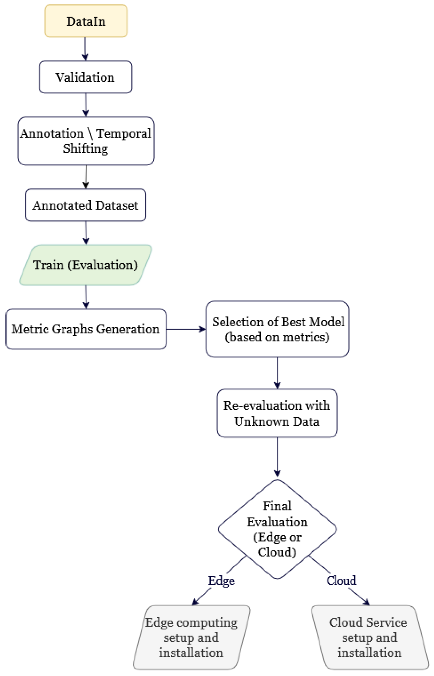
Figure 2.
Sub-models’ architectures: (a) Model 1, (b) Model 2, (c) Model 3, (d) Model 4.
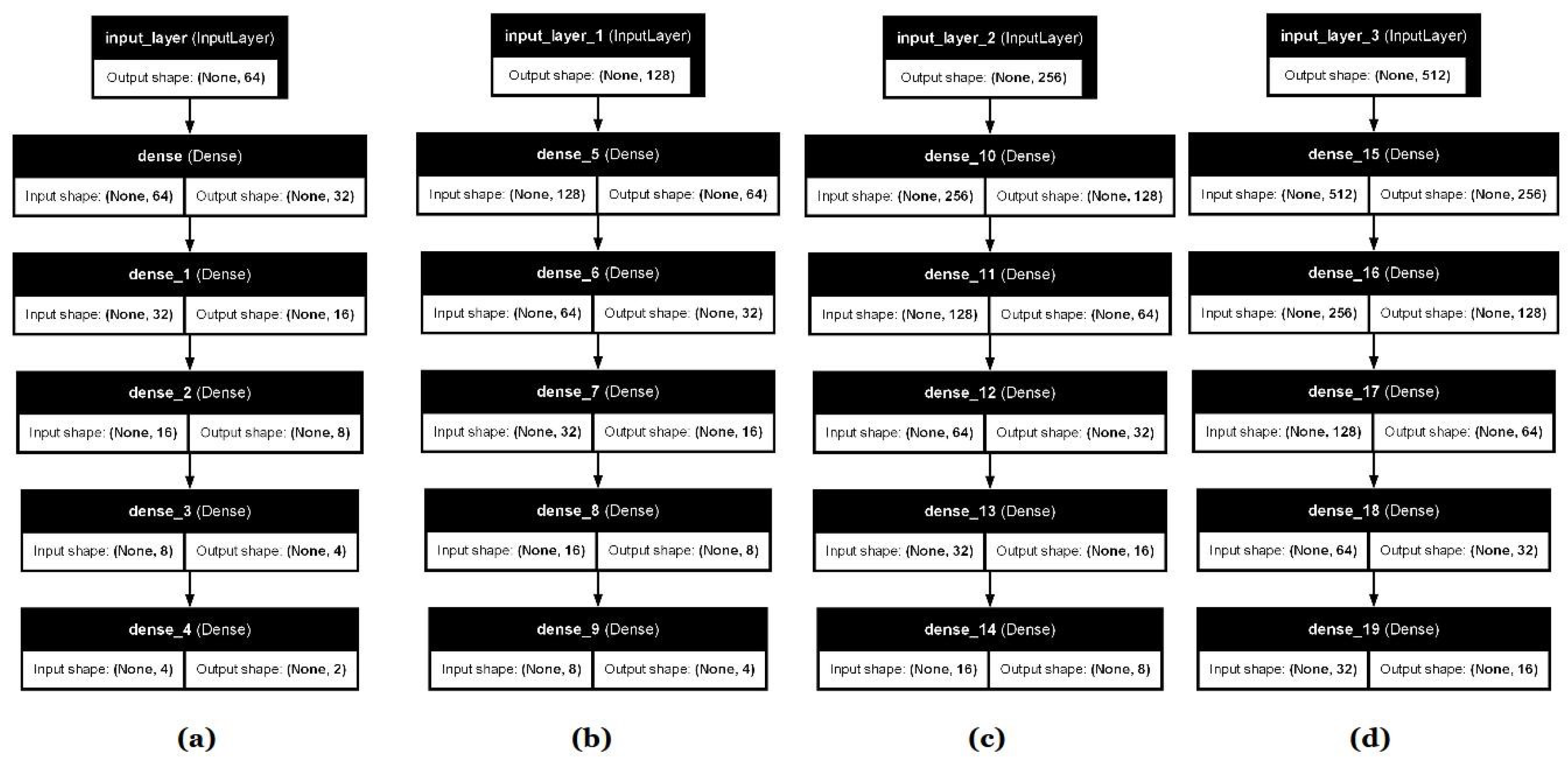
Figure 3.
GRU-model configurations’ architectures for edge case: (a) Config 1: , (b) Config 2: , (c) Config 3: , (d) Config 4: .
Figure 3.
GRU-model configurations’ architectures for edge case: (a) Config 1: , (b) Config 2: , (c) Config 3: , (d) Config 4: .
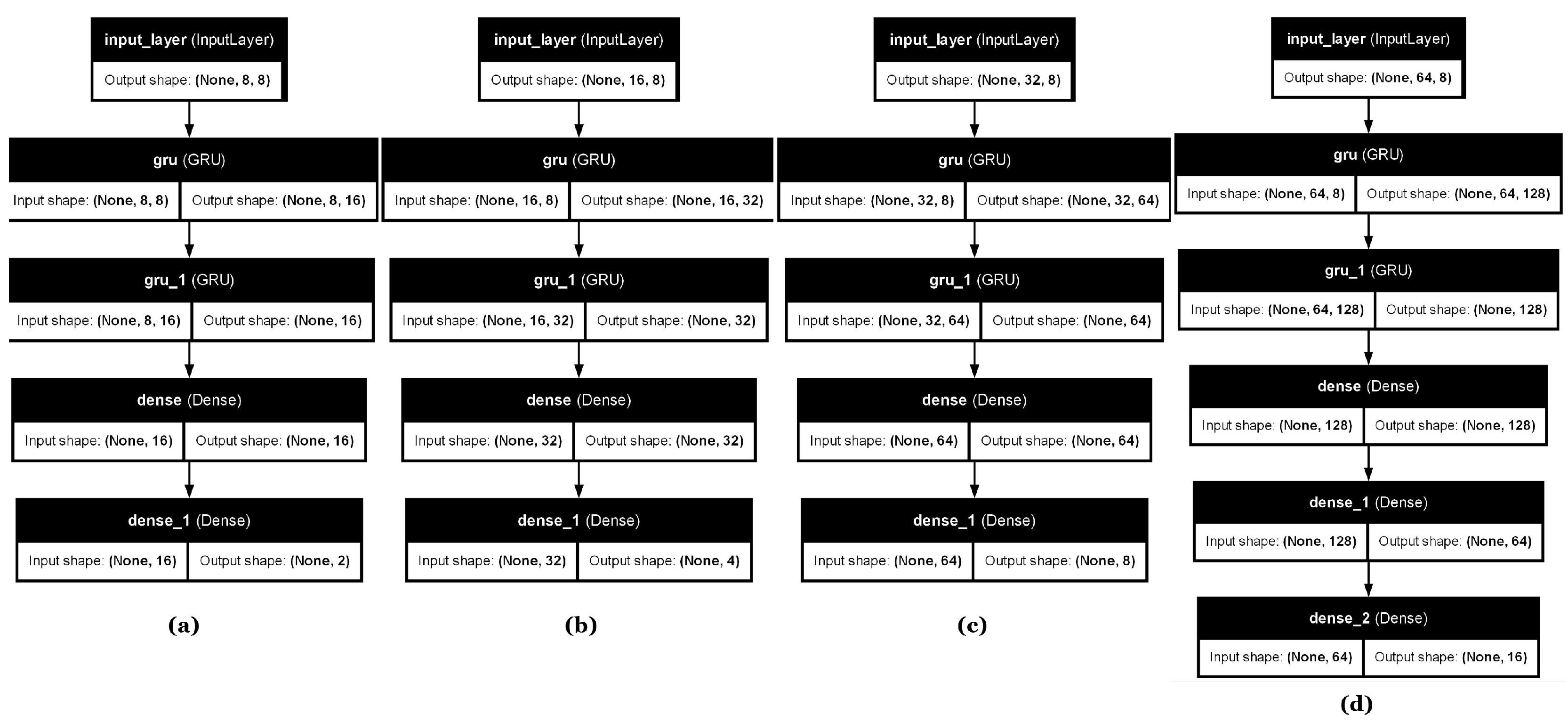
Figure 4.
GRU-model configurations’ architectures for cloud case: (a) Config 1: , (b) Config 2: , (c) Config 3: , (d) Config 4: .
Figure 4.
GRU-model configurations’ architectures for cloud case: (a) Config 1: , (b) Config 2: , (c) Config 3: , (d) Config 4: .
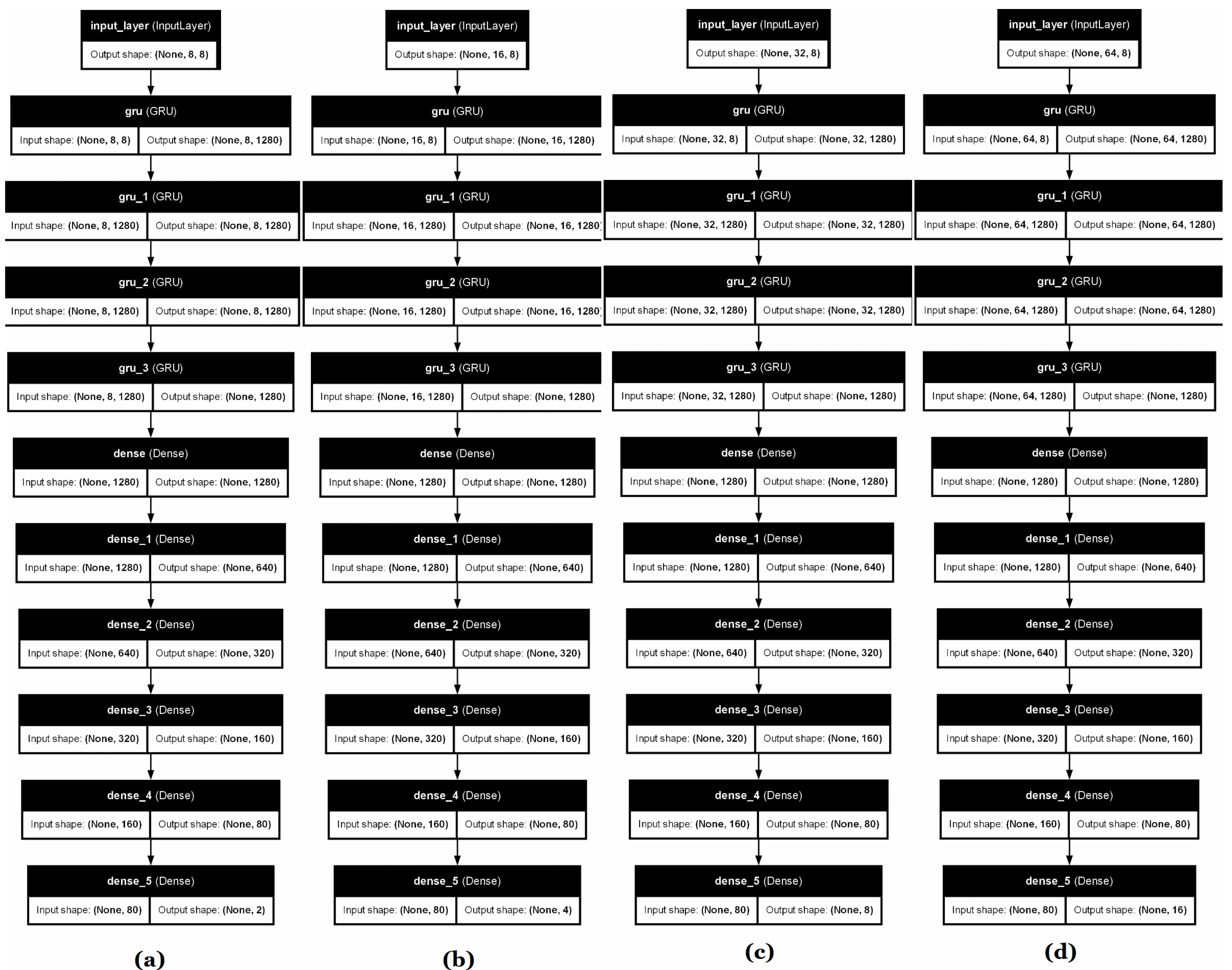
Figure 5.
The reshaping process of each model.As shown in the figure:(a): Model 1, (b): Model 2:, (c): Model 3 and (d): Model 4
Figure 5.
The reshaping process of each model.As shown in the figure:(a): Model 1, (b): Model 2:, (c): Model 3 and (d): Model 4
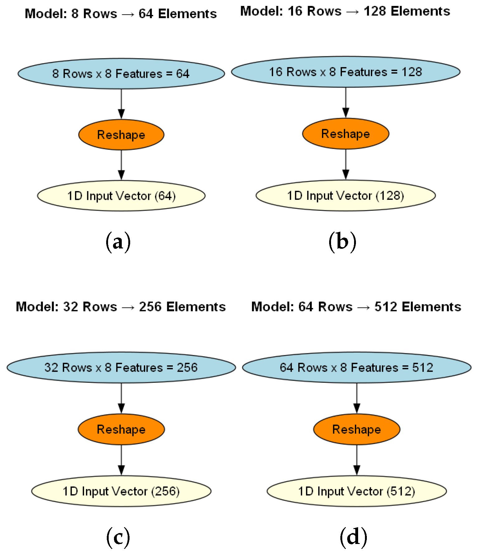
Figure 6.
RMSE values (AQI units) obtained from each of the four input-output configurations on both edge computing model architectures: slideNN and GRU.
Figure 6.
RMSE values (AQI units) obtained from each of the four input-output configurations on both edge computing model architectures: slideNN and GRU.
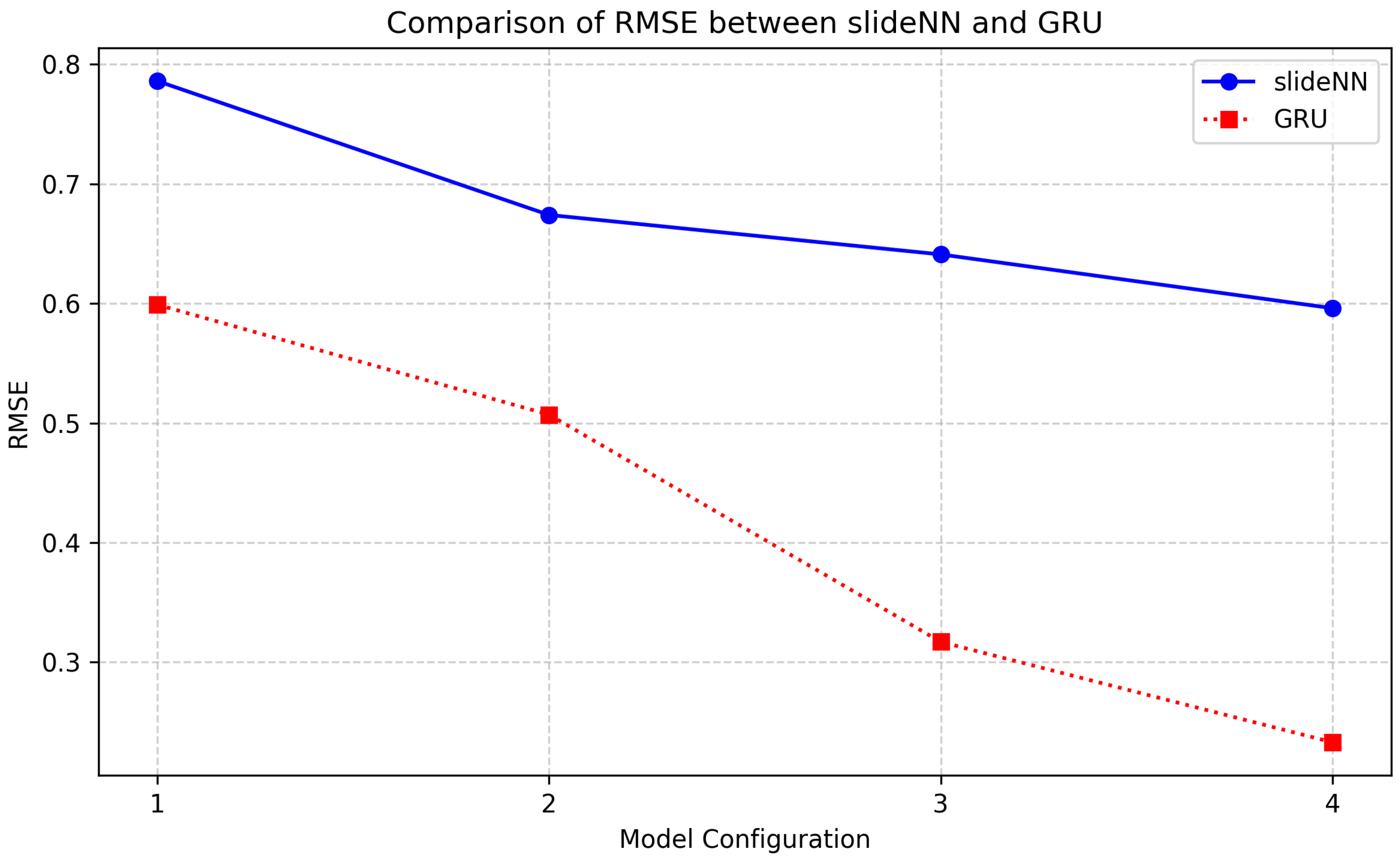
Table 1.
EPA Air Quality Index (AQI) Categories and Health Implications.
| AQI Range | Category | Color Code | Health Implications |
|---|---|---|---|
| 0–50 | Good | Green | Air quality is considered clean with minimum dist or particulate matter. |
| 51–100 | Moderate | Yellow | Acceptable; some pollutants may affect a few particularly sensitive individuals. |
| 101–150 | Unhealthy for Sensitive Groups | Orange | Members of most sensitive groups may experience health issues. Nevertheless, the general public is unlikely to be affected. |
| 151–200 | Unhealthy | Red | All groups (sensitve-non sensitive) may begin to experience health effects. Sensitive groups may experience them more severely. |
| 201–300 | Very Unhealthy | Purple | Health alert: Everyone may experience serious health effects. |
| 301–500 | Hazardous | Maroon | Health warnings of emergency health conditions. |
Table 2.
Overview of hyperparameters for all models.
| slideNN (Edge Computing) | |||||
|---|---|---|---|---|---|
| Submodel | Input Length | Output Length | Learning Rate | Epochs | Batch Size |
| 1 | 64 | 2 | 0.0008 | 400 | 32 |
| 2 | 128 | 4 | |||
| 3 | 256 | 8 | |||
| 4 | 512 | 16 | |||
| GRU Model (Edge Computing) * | |||||
| GRU cells | Input Length | Output Length | Learning Rate | Epochs | Batch Size |
| 16 | 64 | 2 | 0.001 | 50 | 32 |
| 32 | 128 | 4 | |||
| 64 | 256 | 8 | |||
| 128 | 512 | 16 | |||
| GRU Model (Cloud Computing)** | |||||
| GRU cells | Input Length | Output Length | Learning Rate | Epochs | Batch Size |
| 1280 | 64 | 2 | 0.0007 | 25 | 32 |
| 128 | 4 | ||||
| 256 | 8 | 0.0005 | 35 | ||
| 512 | 16 | ||||
* All GRU configurations in the edge-case scenario used exactly 2 hidden layers. ** All GRU configurations in the cloud-case scenario used exactly 4 hidden layers
Table 3.
Input-output configurations used across both model architectures. Each configuration represents a specific combination of input window size and prediction horizon applied to both slideNN and GRU models.
Table 3.
Input-output configurations used across both model architectures. Each configuration represents a specific combination of input window size and prediction horizon applied to both slideNN and GRU models.
| Configuration | Input Window (Hours) | Sampling Step (Hours) | Number of Outputs |
|---|---|---|---|
| Config 1 | 64 | 8 | 2 |
| Config 2 | 128 | 16 | 4 |
| Config 3 | 256 | 32 | 8 |
| Config 4 | 512 | 64 | 16 |
Note: These configurations were implemented as separate sub-models in the slideNN architecture and as adjustable hyperparameter scenarios within a single GRU model.
Table 5.
Performance metrics for each sub-model of the slideNN architecture.
| Submodel (Input → Output) | RMSE | MSE |
|---|---|---|
| 64 → 2 | 0.786 | 0.617 |
| 128 → 4 | 0.674 | 0.454 |
| 256 → 8 | 0.641 | 0.410 |
| 512 → 16 | 0.596 | 0.355 |
Table 6.
Performance metrics for each configuration of the GRU architecture.
| Configuration (Input → Output) | RMSE | MSE |
|---|---|---|
| 64 → 2 | 0.599 | 0.369 |
| 128 → 4 | 0.507 | 0.262 |
| 256 → 8 | 0.317 | 0.101 |
| 512 → 16 | 0.233 | 0.055 |
Table 7.
Model configurations with parameter count and the corresponding memory size.
| Configurations | Input/Output Size | Parameters (p) | Memory (MB) |
|---|---|---|---|
| 1 | 64/2 | 37,196,882 | 141.89 |
| 2 | 128/4 | 37,197,044 | 141.9 |
| 3 | 256/8 | 37,197,368 | 141.9 |
| 4 | 512/16 | 37,198,016 | 141.9 |
Table 8.
Performance metrics for each configuration of the GRU architecture.
| Configuration (Input → Output) | RMSE | MSE |
|---|---|---|
| 64 → 2 | 0.468 | 0.226 |
| 128 → 4 | 0.334 | 0.114 |
| 256 → 8 | 0.213 | 0.046 |
| 512 → 16 | 0.201 | 0.041 |
Disclaimer/Publisher’s Note: The statements, opinions and data contained in all publications are solely those of the individual author(s) and contributor(s) and not of MDPI and/or the editor(s). MDPI and/or the editor(s) disclaim responsibility for any injury to people or property resulting from any ideas, methods, instructions or products referred to in the content. |
© 2025 by the authors. Licensee MDPI, Basel, Switzerland. This article is an open access article distributed under the terms and conditions of the Creative Commons Attribution (CC BY) license (http://creativecommons.org/licenses/by/4.0/).
Copyright: This open access article is published under a Creative Commons CC BY 4.0 license, which permit the free download, distribution, and reuse, provided that the author and preprint are cited in any reuse.


