Submitted:
06 June 2025
Posted:
09 June 2025
You are already at the latest version
Abstract
Accurate landslide displacement prediction is an essential component of landslide early warning systems. The Bazimen landslide in the Three Gorges reservoir area was taken as a case study. In recent years, the outstanding performance of dynamic and static models has attracted the attention of many scholars. Static machine learning algorithm—support vector regression (SVR) and dy-namic machine learning algorithm—long short-term memory neural network (LSTM) were used to predict landslide displacement in this study. At first, to predict landslide displacement accu-rately, the moving average method was used to decompose the cumulative displacement into two components: trend and periodic terms. Second, by introducing the K-Nearest Neighbor (KNN), the forecast results of SVR and LSTM models were classified with greater accuracy based on the se-lection of input factors. Finally, we proposed a static-dynamic ensemble landslide displacement predic-tion model optimized with KNN to address the dynamic characteristics of landslide evo-lution and the shortcomings of traditional static prediction models. Through the out-put of the KNN model, the results of the static-dynamic coupling model are updated to get the KNN-optimized SVR-LSTM landslide displacement prediction model. Compared with traditional landslide displacement prediction models that output prediction values, this study optimized the prediction results through a classification algorithm. The results show that the LSTM models show better performance than the SVR models: For monitor-ing point ZG111, the values of RMSE and MAPE with the SVR model were 30.71 mm and 2.15%, while the accuracy factors of the LSTM model were 24.73 mm and 1.87% and the values of RMSE and MAPE with the Ensemble model were 23.11 mm and 1.68%. It can be seen that the ensemble model integrates the advantages of static (SVR) and dynamic (LSTM) models, and its prediction performance is better than that of the single SVR model and the LSTM model. This study provides an integrated view of the landslide displace-ment pre-diction model, which can provide a reference for predicting geological disasters in the Three Gorges reservoir area.
Keywords:
Bazimen landslide
; landslide displacement prediction
; K-Nearest neighbor
; support vector re-gression
; long short-term memory neural networks
; integration algorithm
1. Introduction
Landslides are responsible for causing significant casualties and property losses worldwide [1]. A method that can effectively predict landslide displacement is necessary. However, the environment where landslides occur often has complexity and diversity. Therefore, predicting landslide displacement is a challenging but essential work for dis-aster reduction. At the same time, selecting an appropriate displacement prediction model is paramount [2]. In the past 20 years, many researchers have studied the implementation of intelligent algorithms in landslide displacement prediction [3,4].
Researchers have developed various methods to predict landslide displacement. Du et al. [5] discussed applying a backpropagation neural network model in predicting ac-cumulation layer landslide displacement. Liu et al. [6] explored the potential of several machine learning algorithms and found that deep learning algorithms, such as LSTM and GRU, displayed the most promising results for predicting ground displacement under three types of landslides. Finding an integrated model with more robust adaptability and better generalization ability has been a critical focus of current landslide displacement prediction research [7].
The organization of the input data is another significant aspect of implementing the prediction models. In the time series study of landslide displacement, Li et al. [8] divided cumulative displacement time series into trend items and periodic items using the Ho-drick-Prescott filtering method. A polynomial model was used to forecast trend items, while periodic items were forecast using the limit learning machine and least squares support vector machine methods. Jia et al. [9] decomposed displacement into two compo-nents using a time series model. Researchers employed a particle swarm optimiza-tion-optimized least squares support vector machine model to forecast landslide dis-placement by analyzing rainfall and reservoir water levels.
Regarding factor screening and model evaluation, researchers mainly use mutual information value, Pearson correlation coefficient, and grey correlation analysis method [10] to screen input factors. The root mean squared error (RMSE) and the mean absolute percentage error (MAPE) are mostly used to evaluate forecast accuracy.
In addition, at this stage, there is plenty of research on the static prediction model SVR and the dynamic prediction model LSTM. Li et al. [11] proposed a dynamic predic-tion model of landslide displacement based on singular spectrum analysis (SSA) and stacked long short-term memory (SLSTM) network for the dynamic characteristics of landslide evolution and the shortcomings of the traditional static prediction model. Lin et al. [12] analyzed the inherent relationship between rainfall, reservoir water level, and pe-riodic displacement of landslide. They put forward a dynamic landslide displacement prediction model based on time series analysis and a two-way long short-term memory model (Double-BiLSTM). Zhang et al. [13] proposed a composite dynamic model for the prediction of landslide displacement based on the empirical mode decomposition soft screening stopping criterion (SSSC-EMD) and deep bidirectional long short-term memory (DBi-LSTM) neural network, which can better characterize the "stepped" deformation characteristics of the slope. Jiang et al. [14] comprehensively utilized the advantages of several algorithms and performed integrated model research based on linear weight. It can be seen from the above research that the optimization direction of the prediction of landslide displacement is mainly based on the innovation of the displacement decompo-sition algorithm and the optimization of hyperparameters of the prediction algorithm. In contrast, the research on the integrated algorithm is less in the past decade.
It is necessary to find a new method that focuses on an integrated algorithm to pre-dict the displacement of landslides. In this paper, we preprocessed the displacement monitoring data of the Bazimen landslide and selected 84 time-step data for research. Cumulative displacement decomposition is an additive decomposition divided into two parts: trend displacement and periodic displacement, respectively [15]. We decomposed the displacement monitoring data into trend items and period items; the trend items were predicted by single variable method, and the period items were predicted by multivariable method. The total displacement prediction results are obtained by summing the predicted values of the trend item and period item based on the static machine learning algorithm SVR and dynamic machine learning algorithm LSTM. Finally, the KNN algorithm is used to establish the classifier of the optimal prediction model, and the output of the KNN al-gorithm is optimized to realize the optimization of the static-dynamic coupling model and integrate the forecasting advantages of the static-dynamic model. The overall process is shown in Figure 1.
2. Methodology
2.1. Decomposition of the Displacement Time Series into Trend and Periodic Terms
The scientific decomposition of trend and periodic items is the basis for establishing reliable models [16].In this paper, the original displacement of the landslide will be de-composed into two components, namely the trend term and the period term [17]. Land-slide trend items are affected by the geological conditions of the landslide itself, such as geological tectonism, weathering, etc., and are also related to the deformation evolution stage of the landslide. It is significant to analyze the effect of influencing factors on land-slide prediction and development [12]. The periodic term of the landslide corresponds to the short-term displacement of the wading landslide in the Three Gorges reservoir area, which is mainly influenced by two factors: the change in rainfall and the change in the level of reservoir water [18]. The displacement caused by random factors is difficult to monitor and relatively small, which is not considered in this study. The accumulated dis-placement time series can be decomposed as follows:
where is the time step, is the accumulated displacement, is the trend term, and is the periodic term.
2.2. Moving Average Methods
The moving average method used in this paper is to smoothen the time series data to achieve smoothness and then to accurately determine the period series and its influencing factors, to achieve more effective trend prediction. The function of the single-moving aver-age method is shown as follows:
whereis the trend term of the displacement at the time step t, is the cumulative displacement of the landslide at the time step t, and n is the moving average cycle. In this paper, the moving average period adopts 12, because the reservoir water level dispatching in the Three Gorges reservoir area takes 12 months as a period.
2.3. Support Vector Regression
In machine learning, support vector regression (SVR) is a supervised learning model with relevant learning algorithms, which can be used to analyze data for classification and analysis [19]. Therefore, it is a machine learning method based on minimizing structural risk [20]. This method can solve the problems of low-sample, high-dimensional nonlinearity, and local minimum [21]. In SVR models, a given sample data (k is the number of sample data) for dealing with regression problems is divided into a fitting sample and a predicting sample [22]. The fitting samples are mapped to a high-dimensional feature space where the optimal linear regression function is constructed [23]. The regression function for SVR is:
where W is the weight vector, is a nonlinear mapping from the input space to the output space, b is bias. Considering the fitting error, with the introduction of relaxation factors, the optimization problem of SVR can be converted into the following:
where C is the penalty factor; is an insensitive loss function.
Standard kernels include radial basis function (RBF) kernels, linear kernels, polynomial kernels [17]. The RBF is widely used with its broad convergence domain. In this study, we selected RBF kernels for the SVR model.
2.4. Long Short-Term Memory Neural Networks
Recurrent neural networks (RNNs) (Figure 2. a) have achieved great success and have been widely used in many Natural Language Processing (NLP) [24]. RNNs contain input units, the input set is marked as, and the output set of the output units is marked as. RNNs also contain hidden units, whose output set is marked as.
St is the state of the hidden layer at time step t. It is calculated based on the output of the current input layer and the status of the previous hidden layer. Where f is generally a nonlinear activation function.
However, in practice, RNNs are not capable of solving a problem as long-term de-pendencies, for the vanishing-gradient or exploding-gradient problems. The LSTM neural network, as a particular type of RNN, can learn long-term dependencies (Figure 2.b). LSTM replaces each unit in RNN with a memory block. There are three gate functions in this memory block. The input gate controls the input activation flow to the memory unit, while the output gate controls the output flow to other units or as a final result.
The layer of the forget gate determines the information discarded about the status of the cell by looking at (the previous output) and (the current input) and outputting numbers between 0 and 1 for each digit of the cell state (the previous state). 1 represents complete retention, while 0 represents complete deletion. The combination of the three types of gates controls the output state. The critical difference between RNN and LSTM is the expression of hidden vectors ht. The hidden vector ht in the LSTM neural network can be obtained as follows:
where , , and are the values of the input gate, the forget gate, the output gate, and the memory cell in the memory block; , , and are their corresponding offset values; is the sigmoid function; represents the weight that connects the memory unit to the output node. The above formula's set of results is iterated from times t = 1 to T.
2.5. Reliability Evaluation of the Model
The optimal hyperparameters of the models were obtained through the entire data set of fitting, and then the entire data set of training and the optimal hyperparameters were used to train the models [25]. To verify the prediction accuracy, we calculated the root mean square error (RMSE) [26] and the mean absolute percentage error (MAPE) [27].
where is the measured value; is the predicted value; N is the number of predicted values.
3. Study Site
3.1. Bazimen Landslide
The Bazimen landslide is located on the right bank of the Xiangxi River in Zigui County (Figure 3). The Xiangxi River runs in a north-south direction here and is close to the Yangtze River. The Three Gorges Reservoir submerged the front edge of the landslide at an elevation of 55-135m [28]. The landslide body is located on the right bank of the Xiangxi River, with a north-south trend on the bank slope. The body of the landslide is distributed in a dustpan shape at the foot of the bank slope. The elevation of the distribution of the landslide body is 139m~280m, with a high elevation in the west and a low elevation in the east, including towards the east and showing a stepped undulation. The landslide still has secondary platforms, namely the front edge platform and the rear edge platform, with distribution elevations of 139-165m and 220-230m, respectively.
3.2. Landslide Inventory
The initial monitoring network for the Bazimen landslide was established in June 2003, which includes four GPS deformation monitoring points (ZG111, ZG110, ZG112, ZG109) (Figure 4).
The Bazimen landslide was reactivated after water storage in Gezhouba Reservoir in 1982. Four NW-SE trending cracks developed at a landslide elevation of 80-125 m. Deformation cracks occurred again in the Bazimen landslide in 1983. From May to June 2003, the water level of the Three Gorges Reservoir rose from 80m to 135m, which is the initial stage of landslide deformation. ZG111 showed the largest displacement at the top of the landslide. From July to August 2003, cracks occurred in a landslide. Before the rainy season in May 2004, the reservoir area displacement curve showed a steady growth trend, which shows that the influence of the increase in water level after the first impoundment on the water level in the reservoir area still exists. From May to July 2004, several cracks appeared in the landslide. In June 2005, the deformation of the landslide cracks intensified; From June to July 2007, the deformation rate of the landslide increased. Since then, the water level in the Three Gorges reservoir area has been regulated between 145 and 175 m, with a maximum drop of 30 m between high and low. The detailed annual variation process is shown in the diagram (Table 1).
The deformation characteristics of the Bazimen landslide indicated that the movement is an ‘advancing’ type of landslide, which means that the landslide started from the upper part and developed downward with increasing displacement [29]. Figure 5 depicts the two GPS monitoring stations, ZG110 and ZG111, which were installed on the ground surface in the main section Ⅰ-Ⅰ’ of the Bazimen landslide.
4. Prediction Process
4.1. Point Selection and Data Processing
In this paper, the ZG111 data is selected as the GPS deformation detection point, and the data displacement monitoring data of 84-time steps from January 2004 to December 2010 are taken as the research object.
First, the original data on the displacement of the landslide is decomposed by the moving average method. The dataset is often divided in proportion such as 7:1.5:1.5 or 6:2:2 according to relevant literature on landslide displacement prediction [15,30]. After decomposition, the first 72-time steps are designated as fitting set data. Of these, 60-time steps serve as the training set for model development, 12-time steps function as the verification set for model hyperparameter optimization and adjustment, and the remaining 12-time steps are utilized as the prediction set to assess model performance. The specific situation of the decomposition of the increment of displacement of landslide is shown in Figure 6.
4.2. Factors Selection
The selection of alternative influencing factors and alternative status factors plays a vital role in landslide prediction [30]. The relationship between landslide initial displacement and influencing factors is shown in Figure 7. In this paper, several candidate factors related to rainfall variation and reservoir water level are selected and labeled as f1 to f12 [31]. A grey correlation coefficient with the resolution of 0.5 obtained by the gray correlation analysis method (GCAM). According to the work of researchers, the grey correlation coefficient at a resolution of 0.5 is usually adopted when using GCAM. They concluded that the higher gray correlation coefficient illustrated the strong correlation between two variables. They also pointed out that if the gray correlation coefficient is more significant than 0.6, we can think there is a strong correlation between the two variables. Following the method, we pick up the candidate input factors that obey the principle proposed by Jiang et al. [14]. We list all available input factors in Table 2.
At the same time, based on correlation degree analysis, collinearity analysis on candidate factors is carried out. By excluding input factors with collinearity exceeding the standard, the prediction accuracy of the model is improved. Generally speaking, when tolerance is less than or equal to 0.1 or the variance inflation factor (VIF) is greater than 5, the problem of collinearity exists in the index [32]. The relationship between displacement increment and another issue of ZG111 showed that these factors have an inseparable relationship with each other (Figure 8).
According to the results of the analysis, f7 is screened, and the range of the reservoir water level changes during the current month. f9, the number of days the reservoir water level drops during the current month; f3, the maximum daily rainfall during the current month. So far, the evaluation of input factors has been completed (Table 3).
4.3. Normalization and Inverse Normalization
For machine learning algorithms, normalization, as a fundamental task in data preprocessing, can help them find optimal parameters more easily. Data normalization refers to scaling the data proportionally to fit into a small specific interval [33]. Remove the unit limitation of the data and convert them into dimensionless pure numerical values, facilitating the comparison and weighting of indicators with different units or magnitudes and accelerating the convergence of the training network.
We assumed that the entire fitted set data is known information, and the predicted data set is unknown. Consequently, the boundary values for normalization and inverse normalization should be obtained from the fitted dataset rather than the entire dataset to avoid information leakage.
where is the normalized value, is the original value, is the maximum value of the samples, and is the minimum value of the samples.
4.4. Parameters of SVRs and LSTMs
The SVR models operated in the Python language environment. Using the grid search (GS) method to search for the optimal parameters of the SVR models [34], RBF is used as the kernel function of the SVR models. The kernel coefficient Gamma of RBF and the penalty parameter C are determined by using GS. In GS processing, the search range of gamma is [0.075, 1.075], and the grid step size is 0.075; The search range for C is [1,75], and the grid step size is 1.
For LSTM models, establishment, batch size, the number of neurons, and numbers of layers of LSTM models were decided with the GS method in succession. In GS processing, the batch size range is [1, 20] with a grid step of 1, and the number of neurons is [1, 20] with a grid step of 1. The optimal epochs were obtained with an early-stopping set during the algorithmic process, and the patience of early-stopping was set at 30, which means the algorithmic process will stop when the result has no improvement within 30 steps. The optimal hyperparameters of the final LSTM and SVR models are shown in Table 4.
5. Results
5.1. SVR Models and LSTM Models
The comparison results of predicted displacement and measured displacement obtained using the SVR and LSTM models at point ZG111 are shown in Figure 9 and Table 5. For ZG111, the RMSE and MAPE values with the SVR model were 30.71 mm and 2.15%, while the accuracy factors of the LSTM model were 24.73 mm and 1.87%.
In trend terms, the RMSE values with the SVR and LSTM models in ZG111 were 2.30 and 3.52 mm. In periodic terms, the RMSE values with the SVR and the LSTM models in ZG111 were 28.92 and 23.61 mm (Table 6).
Compared to the last six months, the SVR and LSTM models performed poorly in the first six months, and the LSTM model performed significantly better than the SVR model in the first six months of trend prediction. LSTM models performed significantly better at point a and period b than SVR models in total displacement. However, for these 12 points, the performance of the LSTM model is not necessarily wholly better than that of the SVR model.
5.2. Ensemble Models for the K-Nearest Neighbor
In the previous chapters, we establish four models related to the SVR and LSTM algorithms in Section 3.4. In this section, we will use SVR and LSTM algorithms to predict the entire dataset and obtain the total prediction displacements of ZG111 from January 2004 to December 2010.
The idea behind optimizing the ensemble models using K-Nearest Neighbor was that if the total displacement predicted by the SVR models is closer to the true value, the output is determined to be 1; otherwise, it is determined to be 0 [35]. The total predicted displacement obtained by the LSTM model, the total predicted displacement obtained by the SVR models, and the difference between the two were set as candidate input factors; these three factors (f13, f14, f15) will enter the optimization model as new candidate input factors for prediction. The hyperparameters and optimal inputs of the KNN model used to predict the optimal model are shown in Table 7.
There are 15 candidate input factors for optimizing the model: f1~f15. By using the factor selection method in Section 3.2, the candidate factors are screened, and the optimal input factors for the model are obtained.
A KNN optimization model was used to predict the optimal weight for an ensemble model [36]. In this section, all datasets with 84-time steps of ZG111 were adopted to predict displacements using SVR and LSTM models. Specifically, 60 time-steps of ZG111 were used as a training dataset to fit the models, 12 time-steps of ZG111 were used as a validation dataset to adjust the hyperparameters of the model, and the remaining 12 time-steps of ZG111 were used as a prediction dataset to predict the optimal weight of the ensemble model. As a result, the optimal hyperparameters of the model are obtained (Table 6).
The comparison results of predicted and measured displacements obtained using KNN-optimized models at point ZG111 are shown in Figure 10 and Table 8. For the total displacement term of ZG111, the values of RMSE and MAPE with the Ensemble model were 23.11 mm and 1.68%, while the accuracy factors of the SVR model were 30.71 mm and 2.15%, and the accuracy factors of the LSTM model were 24.73 mm and 1.87%.
Compared to the LSTM and SVR models, the total displacement predicted by the optimized KNN ensemble model is closer to the measured value than any of the individual models in period a’ and period b’. This indicates that when the results of the LSTM and SVR models were different, the Ensemble model optimized by KNN gave greater weight to the model results that were closer to the true values.
6. Discussion
In this paper, the original displacement of the landslide was decomposed into trend and periodic terms without considering stochastic terms. So far, there has been relatively little research on decomposing landslide displacement into random terms, as random terms are induced by many random factors, such as wind load and vehicle load. The random displacement could not be decomposed and predicted by numerically resolving the observed accumulated displacement and time series of a landslide [37]. It is difficult to obtain the factors that affect the random term displacement of landslides through current detection techniques. The development of high-quality models that can predict the random term of landslide displacement in the future should be considered.
So far, many studies have used machine learning technology to predict landslide displacement, including various integrated models [38]. This study established an ensemble model of the coupled LSTM and SVR algorithm based on KNN optimization for prediction, and the ensemble model performed well. At the same time, many studies have also been conducted on landslide displacement prediction using deep learning. To obtain accurate results in predicting landslide displacement, it is necessary to study a more advanced DL algorithm [39]. Therefore, the new method proposed in this paper provides a new idea for deep learning to predict landslide displacement [40].
In this paper, grey correlation analysis and tolerance analysis are used to select the input factors of the SVR and LSTM models. Standard methods for factor screening include the Chi-square test, wrapper packaging method, embedded method, etc. Although factor selection may help improve the precision of model training, the most critical factor is whether the model trained after factor selection can achieve the expected results when forecasting the forecast set. Screening factors more scientifically and effectively is one of the main directions for future research.
In many studies, the displacement of landslides is often decomposed into two or three components before further prediction processing. If we attempt to directly apply the SVR and LSTM algorithms in this paper without decomposing the landslide displacement, the results obtained are shown in Table 9 and Table 10. It is undesirable to use this decomposition method to predict landslide displacement alone from the results. It can be seen that for accurate displacement prediction, the decomposition of displacement plays a crucial role. In future research, taking the decomposition method in this paper as an example, we need to explore the differences between the trend and periodic components in the original decomposition terms and whether these differences are amplified or decreased in the total displacement after addition calculation.
7. Conclusion
In this paper, we proposed a KNN-optimized SVR-LSTM landslide displacement prediction model. This model was applied to predicting the displacement of the Bazimen landslide in the Three Gorges reservoir area and compared with single models such as the SVR and LSTM models, achieving reliable results. Based on the above research, the following conclusions can be drawn:
(1) Overall, the LSTM model was better than the SVR model, but its results were only sometimes closer to the original values than those of the SVR model at all time steps of the prediction dataset.
(2) The SVR-LSTM landslide displacement prediction model optimized by KNN in this paper combined the advantages of the LSTM and SVR algorithms. The SVR-LSTM model optimized by KNN is closer to the original value in 8-time steps than at least one result in the LSTM or SVR model. Therefore, its prediction performance is considered better than that of the LSTM and SVR models, and the relationship between landslide displacement and factors can be constructed effectively.
The method proposed in this paper combined time series analysis, the LSTM algorithm, the SVR algorithm, the KNN algorithm, and classification prediction theory or method to accurately predict the displacement of the Bazimen landslide in the Three Gorges reservoir area. Research suggested that the integrated model established by this method has the potential to be applied to predict the displacement of landslides in the Three Gorges reservoir area or other areas prone to landslides.
Author Contributions
Conceptualization, H.J. and H.Z.; methodology, H.J. and H.Z.; software, H.J., J.W and H.Z.; formal analysis, H.J. and H.Z.; investigation, H.J., Y.W and H.Z.; visualization, H.J., M.L., S.L and H.Z.; writing—original draft preparation, H.J., H.Z. and J.W.; writing—review and editing, Y.W. and Y.G. All authors have read and agreed to the published version of the manuscript.
Funding
The research work was funded by the Research Fund of National Natural Science Foundation of China (NSFC) (Grant No. 52404113); the Changzhou Sci&Tech Program (Grant No. CJ20240042); the Open Fund of Badong National Observation and Research Station of Geohazards (No. BNORSG-202408); and the high-level Talent Introduction Project of Changzhou University(Grant No. ZMF22020036).
Data Availability Statement
: The original contributions presented in this study are included in the article. Further inquiries can be directed to the corresponding author.
Acknowledgments
The authors thank the National Cryosphere Desert Data Center (http://www.ncdc.ac.cn) for providing the data from the landslide monitoring site for this article and for their strong support for this research. We also sincerely like to thank our group members for their contributions to experimental ideas and help with problems that arose during the experiments, which significantly accelerated the research process.
Conflicts of Interest
The authors declare no conflicts of interest.
References
- Zeng, T.; Yin, K.; Jiang, H. Groundwater level prediction based on a combined intelligence method for the Sifangbei landslide in the Three Gorges Reservoir Area. Sci. Rep. 2022, 12, 11108. [CrossRef]
- Li, X.; Li, Q.; Wang, Y. Effect of slope angle on fractured rock masses under combined influence of variable rainfall infiltration and excavation unloading. J. Rock Mech. Geotech. Eng. 2024, 16, 1-20. [CrossRef]
- Xu, J.; Jiang, Y.; Yang, C. Landslide Displacement Prediction during the Sliding Process Using XGBoost, SVR and RNNs. Appl. Sci. 2022, 12. [CrossRef]
- Zhang, J.; Chen, C.; Wu, C. Development of An Image-based Borehole Flowmeter for Real-time Monitoring of Groundwater Flow Velocity and Direction in Landslide Boreholes. IEEE Sens. J. 2024, 1-1. [CrossRef]
- Zhang, J.; Lin, C.; Tang, H. Input-parameter optimization using a SVR based ensemble model to predict landslide displacements in a reservoir area-A comparative study. Appl. Soft Comput. 2024, 150. [CrossRef]
- Liu, Z.; Guo, D.; Lacasse, S. Algorithms for intelligent prediction of landslide displacements. J. Zhejiang Univ. Sci. A. 2020, 21, 412-429. [CrossRef]
- Zhang, J.; Tang, H.; Zhou, B. A new early warning criterion for landslides movement assessment: Deformation Standardized Anomaly Index. Bull. Eng. Geol. Environ. 2024, 83, 205. [CrossRef]
- Li, D.; Sun, Y.; Yin, K. Displacement characteristics and prediction of Baishuihe landslide in the Three Gorges Reservoir. J. Mt. Sci. 2019, 16, 2203-2214. [CrossRef]
- Zhang, J.; Tang, H.; Tan, Q. A generalized early warning criterion for the landslide risk assessment: deformation probability index (DPI). Acta Geotech. 2024, 19, 2607-2627. [CrossRef]
- Jiang, H.; Wang, Y.; Guo, Z. Landslide Displacement Prediction Stacking Deep Learning Algorithms: A Case Study of Shengjibao Landslide in the Three Gorges Reservoir Area of China. Water. 2024, 16, 3141. [CrossRef]
- Li, L.; Zhang, M.; Wen, Z. Dynamic prediction of landslide displacement using singular spectrum analysis and stack long short-term memory network. J. Mt. Sci. 2021, 18, 2597-2611. [CrossRef]
- Lin, Z.; Sun, X.; Ji, Y. Landslide Displacement Prediction Model Using Time Series Analysis Method and Modified LSTM Model. Electronics. 2022, 11. [CrossRef]
- Zhang, M.; Han, Y.; Yang, P. Landslide displacement prediction based on optimized empirical mode decomposition and deep bidirectional long short-term memory network. J. Mt. Sci. 2023, 20, 637-656. [CrossRef]
- Jiang, H.; Li, Y.; Zhou, C. Landslide Displacement Prediction Combining LSTM and SVR Algorithms: A Case Study of Shengjibao Landslide from the Three Gorges Reservoir Area. Appl. Sci. 2020, 10. [CrossRef]
- Luo, W.; Dou, J.; Fu, Y. A Novel Hybrid LMD–ETS–TCN Approach for Predicting Landslide Displacement Based on GPS Time Series Analysis. Remote Sens. 2022, 15. [CrossRef]
- Zhang, Y.; Tang, J.; He, Z. A novel displacement prediction method using gated recurrent unit model with time series analysis in the Erdaohe landslide. Nat. Hazards. 2020, 105, 783-813. [CrossRef]
- Zhou, C.; Yin, K.; Cao, Y. Application of time series analysis and PSO–SVM model in predicting the Bazimen landslide in the Three Gorges Reservoir, China. Eng. Geol. 2016, 204, 108-120. [CrossRef]
- Yang, B.; Yin, K.; Lacasse, S. Time series analysis and long short-term memory neural network to predict landslide displacement. Landslides. 2019, 16, 677-694. [CrossRef]
- Zhang, Y.; Tang, J.; Cheng, Y. Prediction of landslide displacement with dynamic features using intelligent approaches. Int. J. Min. Sci. Technol. 2022, 32, 539-549. [CrossRef]
- Huang, F.; Cao, Z.; Guo, J. Comparisons of heuristic, general statistical and machine learning models for landslide susceptibility prediction and mapping. Catena. 2020, 191. [CrossRef]
- Chang, Z.; Du, Z.; Zhang, F. Landslide Susceptibility Prediction Based on Remote Sensing Images and GIS: Comparisons of Supervised and Unsupervised Machine Learning Models. Remote Sens. 2020, 12. [CrossRef]
- Ma, J.; Xia, D.; Guo, H. Metaheuristic-based support vector regression for landslide displacement prediction: a comparative study. Landslides. 2022, 19, 2489-2511. [CrossRef]
- Cao, Y.; Yin, K.; Zhou, C. Establishment of Landslide Groundwater Level Prediction Model Based on GA-SVM and Influencing Factor Analysis. Sensors. 2020, 20. [CrossRef]
- Li, H.; Xu, Q.; He, Y. Temporal detection of sharp landslide deformation with ensemble-based LSTM-RNNs and Hurst exponent. Geomatics Nat. Hazards Risk. 2021, 12, 3089-3113. [CrossRef]
- Huang, F.; Yin, K.; Zhang, G. Landslide displacement prediction using discrete wavelet transform and extreme learning machine based on chaos theory. Environ. Earth Sci. 2016, 75. [CrossRef]
- Zeng, T.; Jiang, H.; Li, Q. Landslide displacement prediction based on Variational mode decomposition and MIC-GWO-LSTM model. Stoch. Environ. Res. Risk Assess. 2022, 36, 1353-1372. [CrossRef]
- Zhou, C.; Yin, K.; Cao, Y. A novel method for landslide displacement prediction by integrating advanced computational intelligence algorithms. Sci. Rep. 2018, 8, 7287. [CrossRef]
- Ye, X.; Zhu, H.; Cheng, G. Thermo-hydro-poro-mechanical responses of a reservoir-induced landslide tracked by high-resolution fiber optic sensing nerves. J. Rock Mech. Geotech. Eng. 2023, 16, 1018-1032. [CrossRef]
- Miao, F.; Wu, Y.; Xie, Y. Prediction of landslide displacement with step-like behavior based on multialgorithm optimization and a support vector regression model. Landslides. 2017, 15, 475-488. [CrossRef]
- Wen, H.; Xiao, J.; Xiang, X. Singular spectrum analysis-based hybrid PSO-GSA-SVR model for predicting displacement of step-like landslides: a case of Jiuxianping landslide. Acta Geotech. 2024. 19, 1835-1852. [CrossRef]
- Krkač, M.; Bernat, G.; Arbanas, S. A comparative study of random forests and multiple linear regression in the prediction of landslide velocity. Landslides. 2020, 17, 2515-2531. [CrossRef]
- Ye, C.; Wei, R.; Ge, Y. GIS-based spatial prediction of landslide using road factors and random forest for Sichuan-Tibet Highway. J. Mt. Sci. 2021, 19, 461-476. [CrossRef]
- Li, L.; Wang, C.; Wen, Z. Landslide displacement prediction based on the ICEEMDAN, ApEn and the CNN-LSTM models. J. Mt. Sci. 2023, 20, 1220-1231. [CrossRef]
- Zhang, J.; Tang, H.; Wen, T. A Hybrid Landslide Displacement Prediction Method Based on CEEMD and DTW-ACO-SVR-Cases Studied in the Three Gorges Reservoir Area. Sensors. 2020, 20. [CrossRef]
- Ma, J.; Liu, X.; Niu, X. Forecasting of Landslide Displacement Using a Probability-Scheme Combination Ensemble Prediction Technique. Int. J. Environ. Res. Public Health. 2020, 17. [CrossRef]
- Lin, Z.; Ji, Y.; Liang, W. Landslide Displacement Prediction Based on Time-Frequency Analysis and LMD-BiLSTM Model. Mathematics. 2022, 10. [CrossRef]
- Pei, H.; Meng, F.; Zhu, H. Landslide displacement prediction based on a novel hybrid model and convolutional neural network considering time-varying factors. Bull. Eng. Geol. Environ. 2021, 80, 7403-7422. [CrossRef]
- Ma, Z.; Mei, G. Deep learning for geological hazards analysis: Data, models, applications, and opportunities. Earth-Sci. Rev. 2021, 223. [CrossRef]
- Huang, F.; Zhang, J.; Zhou, C. A deep learning algorithm using a fully connected sparse autoencoder neural network for landslide susceptibility prediction. Landslides. 2019, 17, 217-229. [CrossRef]
Figure 1.
Flow chart of the proposed predictive model.
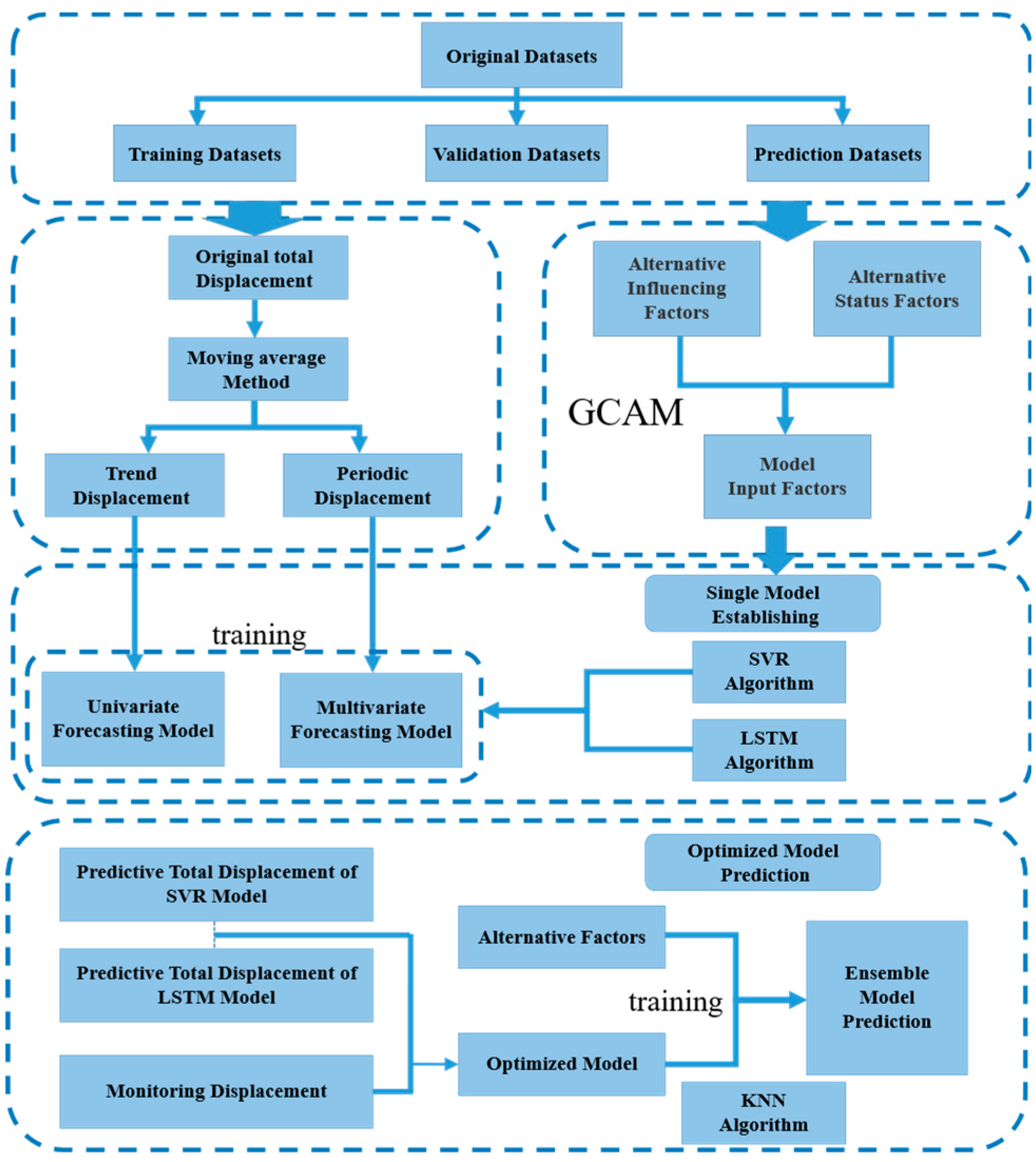
Figure 2.
(a) Standard recurrent neural network (RNN) module contains a single layer. (b) The Long short-term memory (LSTM) module contains four interacting layers.
Figure 2.
(a) Standard recurrent neural network (RNN) module contains a single layer. (b) The Long short-term memory (LSTM) module contains four interacting layers.
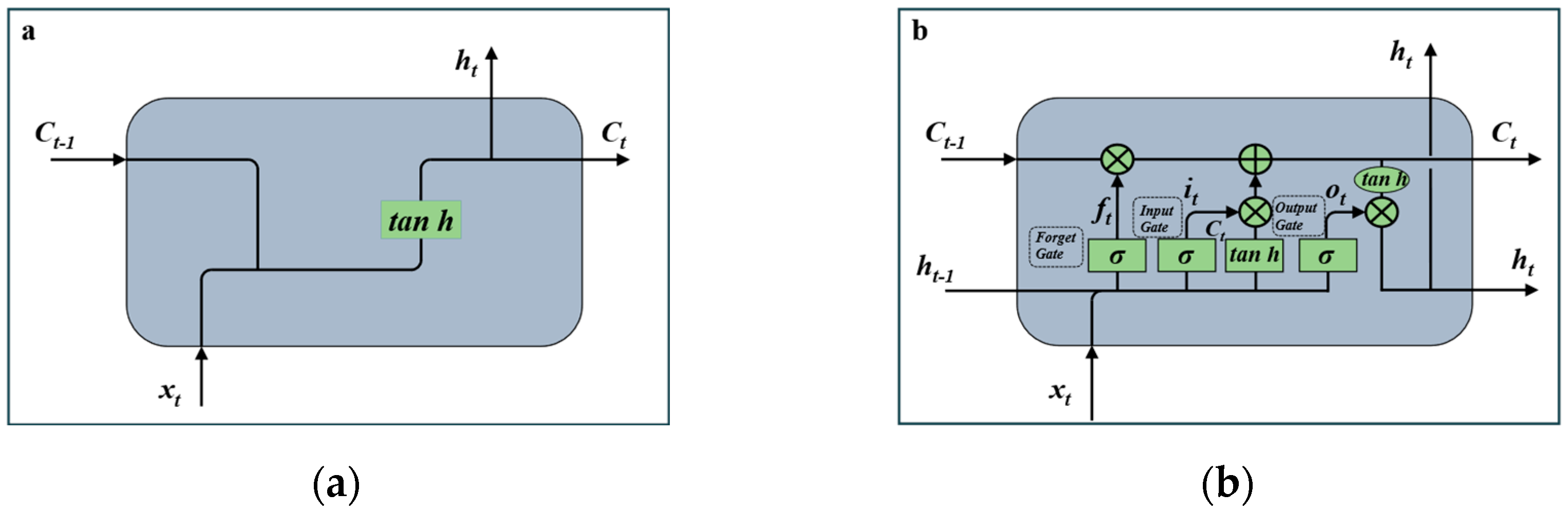
Figure 3.
(a) Location of the Three Gorges Reservoir Area (TGRA) in China; (b) location of the Bazimen landslide;(c) overall view of the Bazimen landslide (satellite image from Google Earth).
Figure 3.
(a) Location of the Three Gorges Reservoir Area (TGRA) in China; (b) location of the Bazimen landslide;(c) overall view of the Bazimen landslide (satellite image from Google Earth).
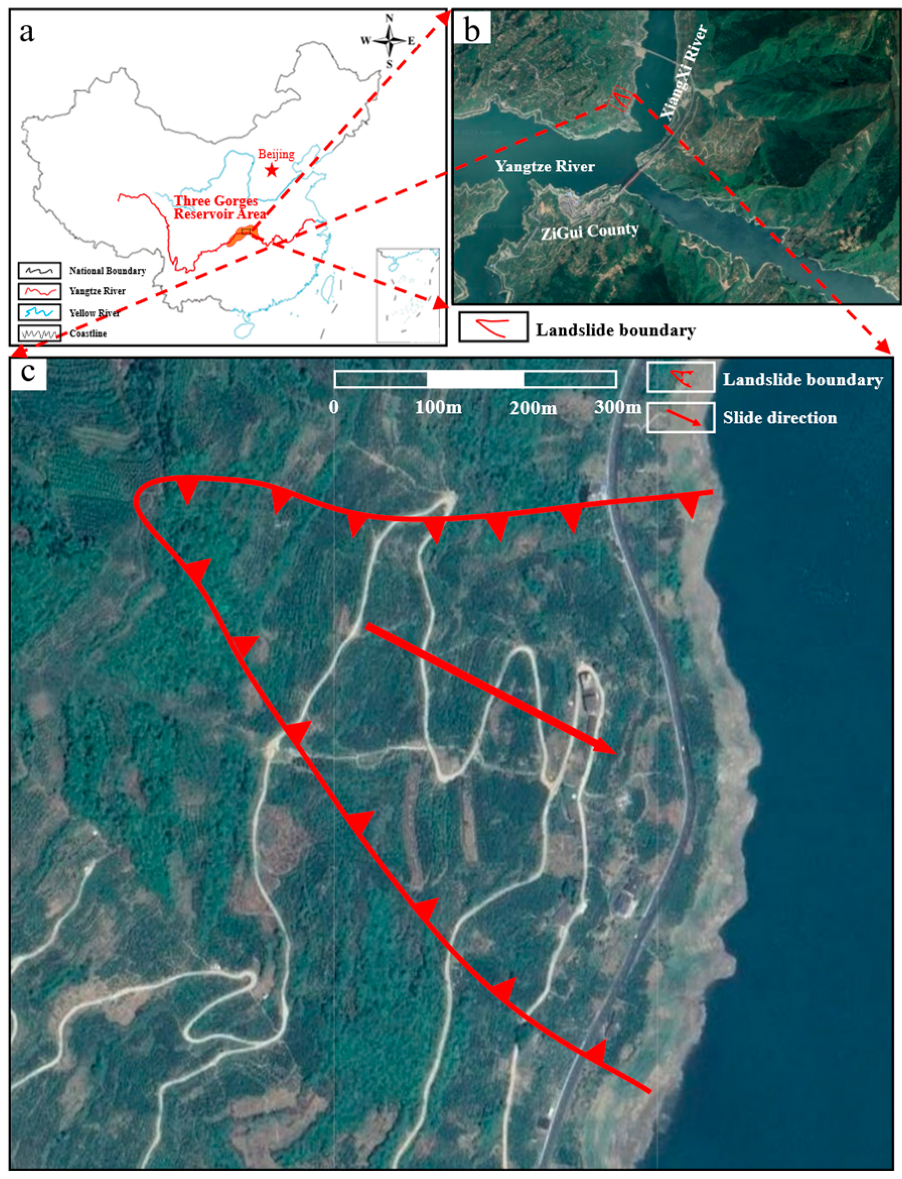
Figure 4.
Monitoring arrangement in the Bazimen landslide and displacement blocks.
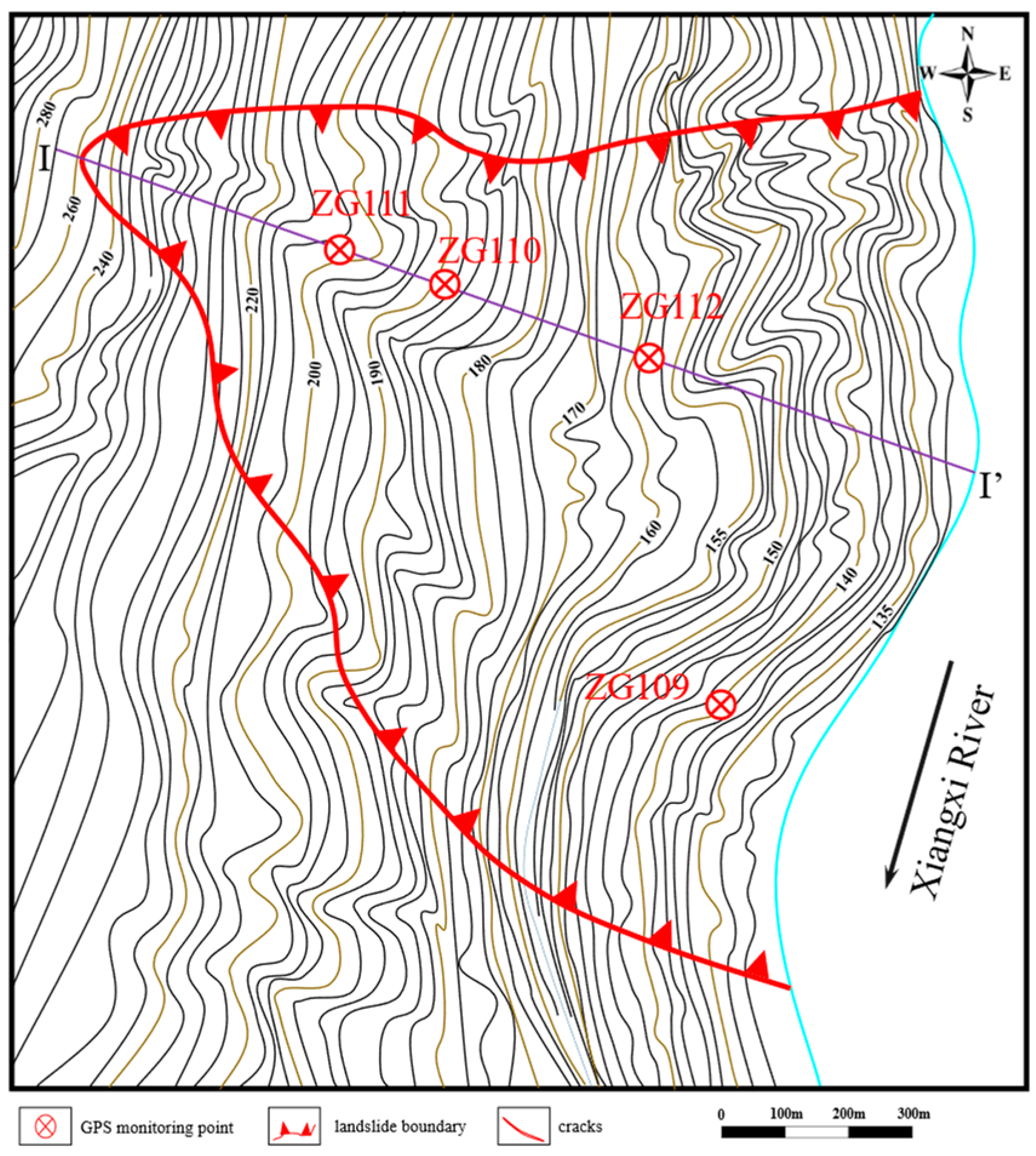
Figure 5.
A Schematic geological cross-section Ⅰ-Ⅰ’ of the Bazimen landslide.
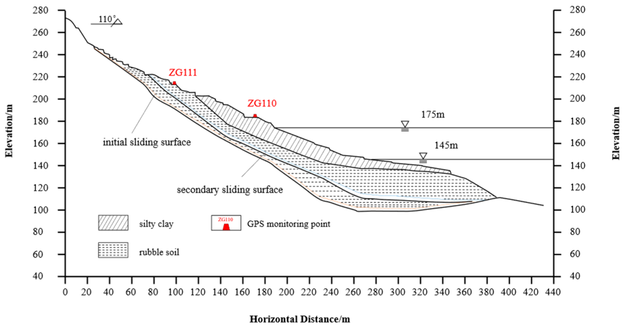
Figure 6.
Results of the decomposition of the displacement monitoring data at the ZG111 point.
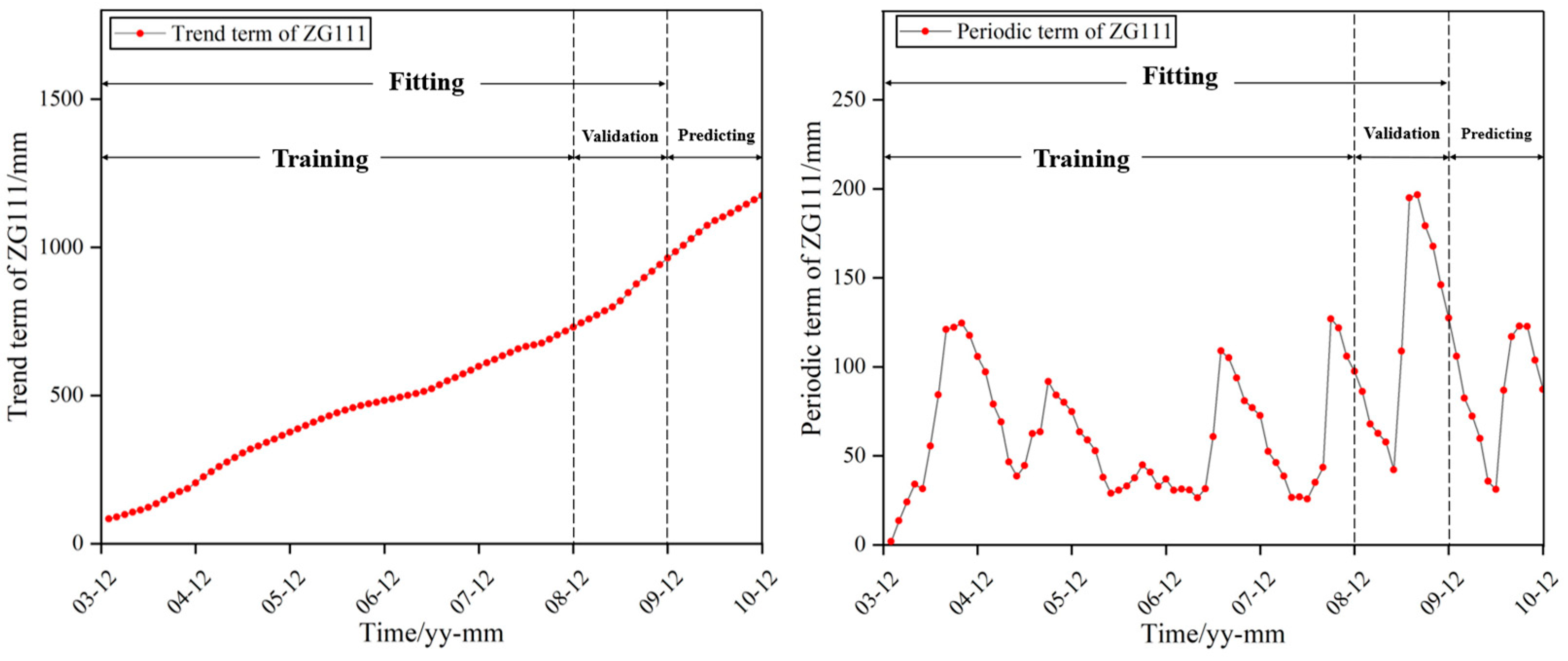
Figure 7.
Rainfall, reservoir water level and cumulative displacement monitoring data from the landslide area.
Figure 7.
Rainfall, reservoir water level and cumulative displacement monitoring data from the landslide area.
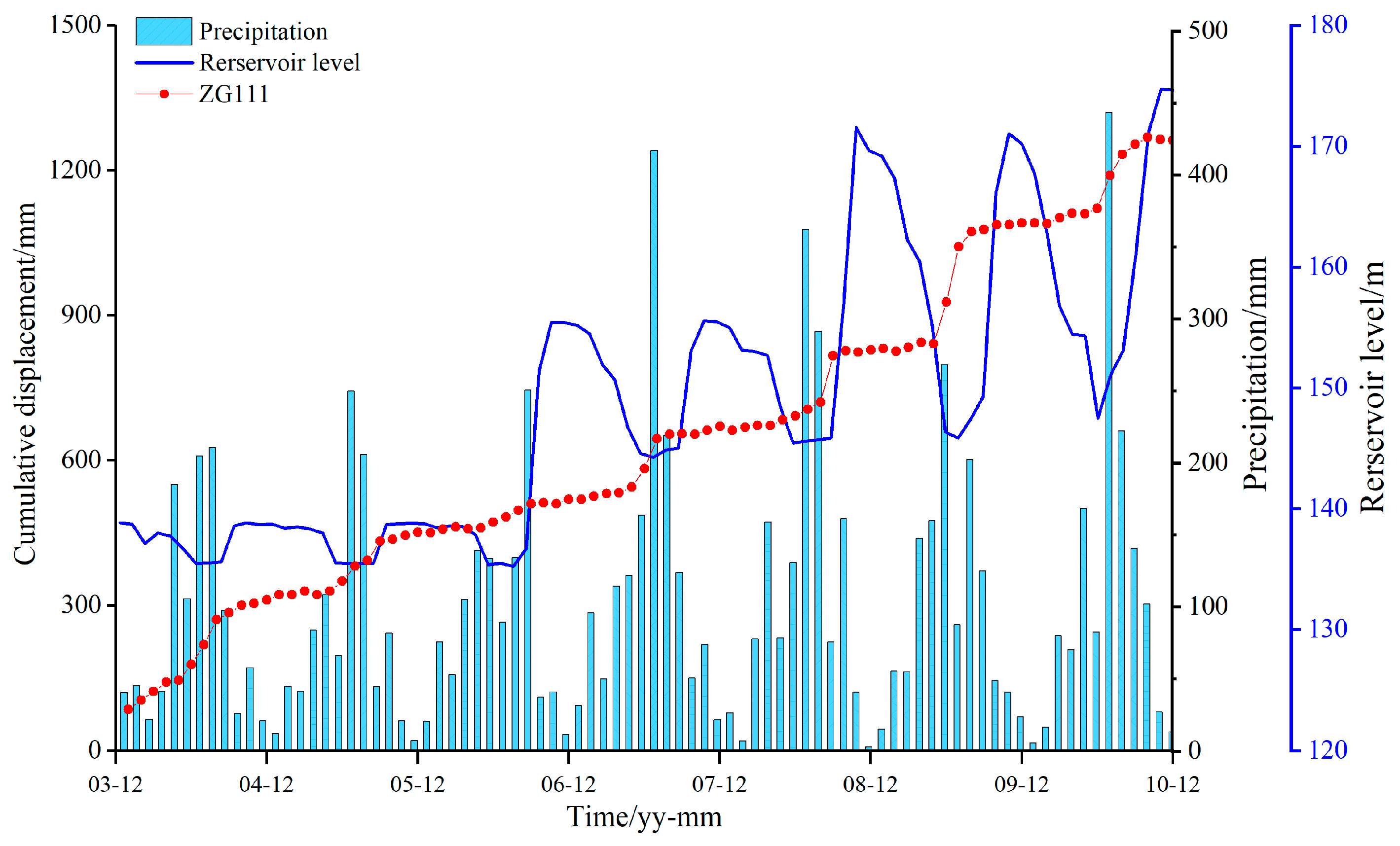
Figure 8.
Rainfall, reservoir water level and displacement increment of ZG111.
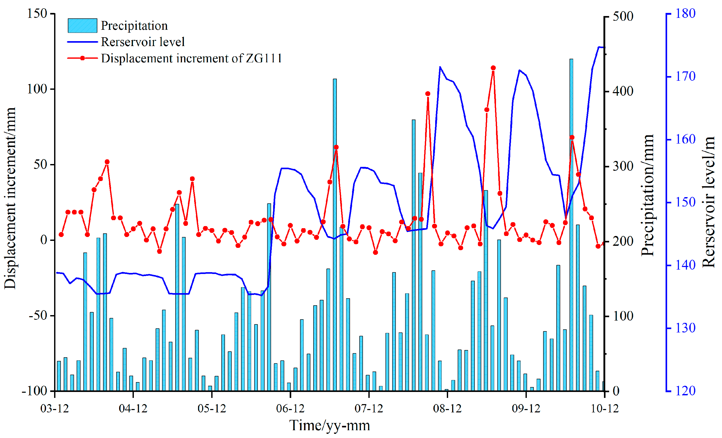
Figure 9.
Curves of the predicted displacement of point ZG111.
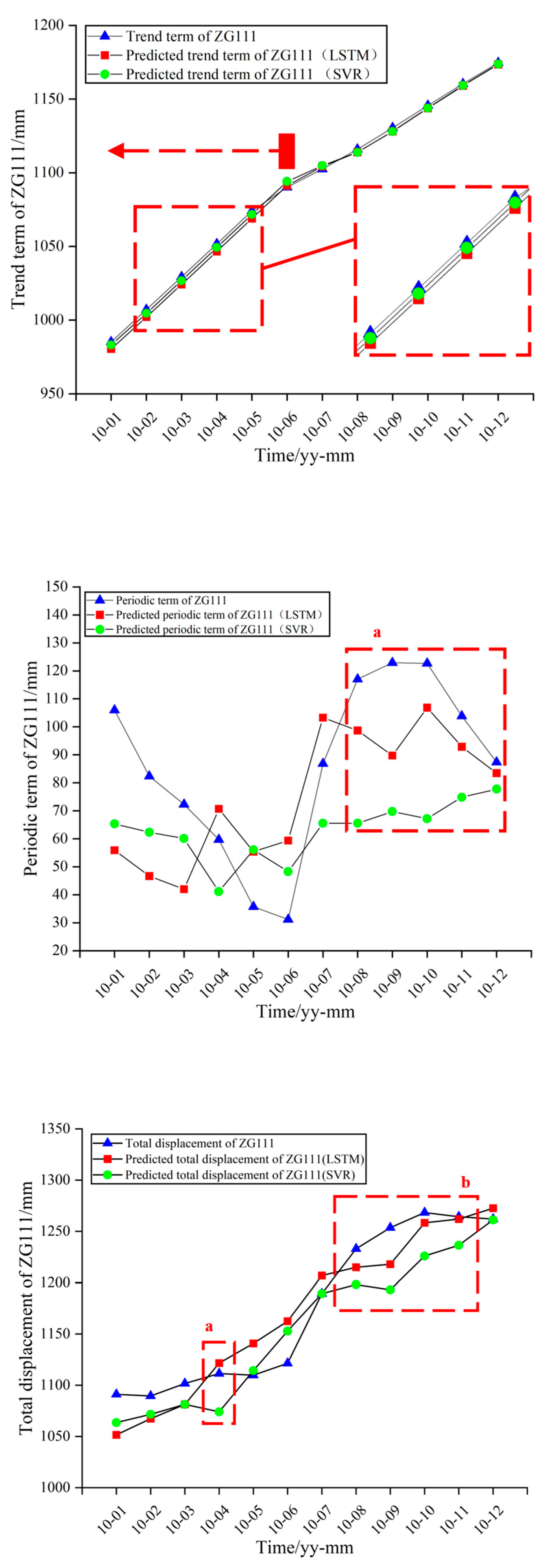
Figure 10.
The curves of the relationship between the observed and predicted displacements.
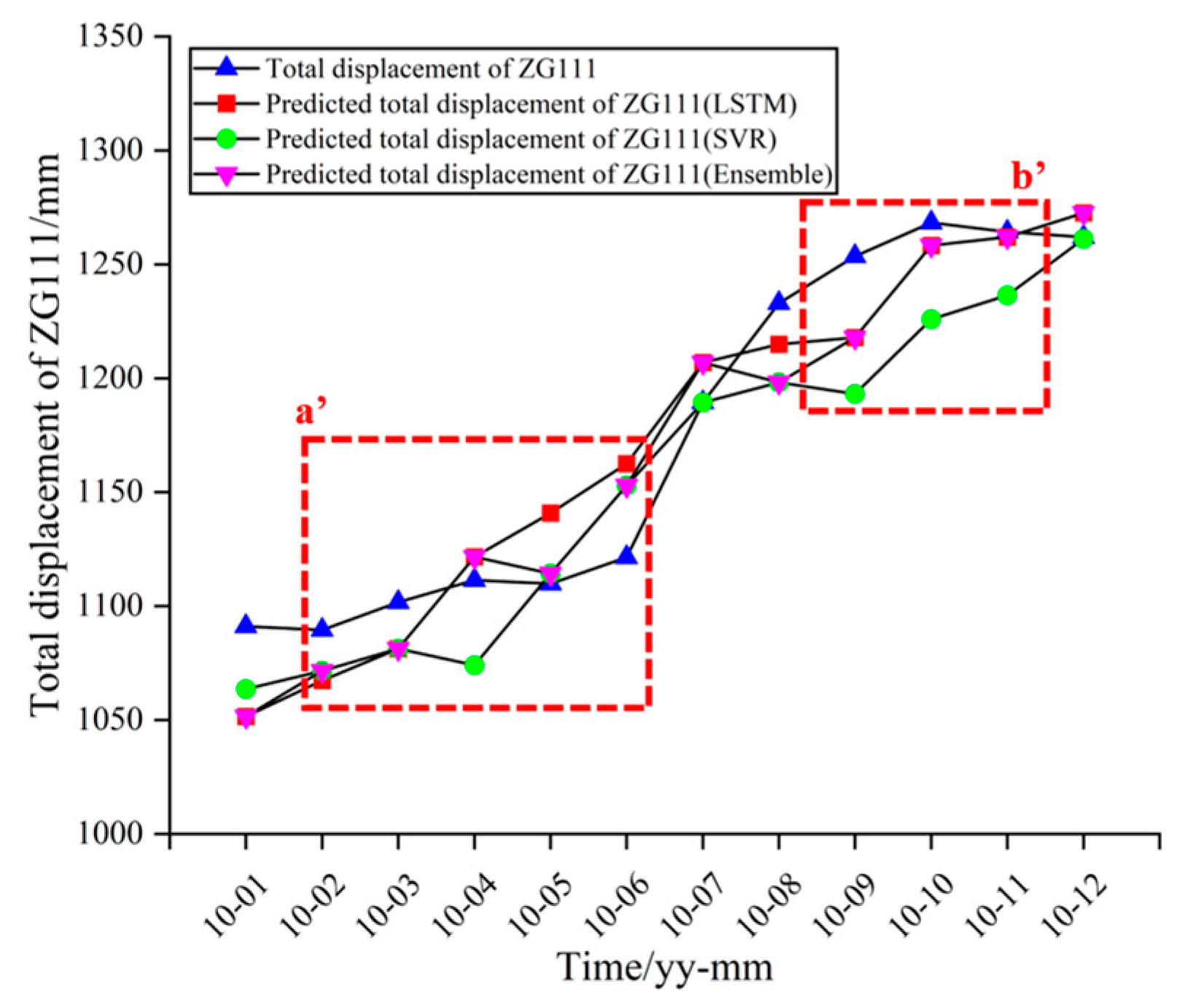

Table 1.
Stages of deformation of the Bazimen landslide.
| Deformation Stage | Time Range | Remarks |
| 1 | March 2003–May 2003 | Landslide deformation starting stage. |
| 2 | June 2003–September 2006 | Cracks begin to appear, the first fluctuation of 135 m. |
| 3 | October 2006–August 2008 | The deformation activity of cracks has intensified, the first fluctuation of 156 m. |
| 4 | September 2008–December 2010 | The first fluctuation of 175 m, the cumulative time-displacement curves with a periodic step-like characteristic. |
Table 2.
Grey correlation coefficient between input factors and periodic displacement of the Bazimen landslide.
Table 2.
Grey correlation coefficient between input factors and periodic displacement of the Bazimen landslide.
| Candidate Factors | Description | ZG111 |
| f1 | the precipitation during the current month | 0.68 |
| f2 | the precipitation during the past two months | 0.63 |
| f3 | the maximum daily rainfall during the current month | 0.65 |
| f4 | the number of rainy days during the current month | 0.63 |
| f5 | the maximum continuous rainfall days during the current month | 0.67 |
| f6 | the average reservoir level during the current month | 0.63 |
| f7 | the change of the reservoir level during the current month | 0.73 |
| f8 | the change of the reservoir level during the past two months | 0.67 |
| f9 | the number of days of reservoir water level decline during the current month | 0.68 |
| f10 | the accumulated decrease in reservoir water level during the current month | 0.69 |
| f11 | the number of days of reservoir water level rise during the current month | 0.64 |
| f12 | the accumulated increase in reservoir water level during the current month | 0.63 |
Table 3.
The result of the collinearity test in ZG111.
|
Candidate Factors |
Initial input factor | New input factor 1 | New input factor 2 | |||||
| Tolerance | VIF | Tolerance | VIF | Tolerance | VIF | |||
| f1 | 0.147 | 6.820 | 0.148 | 6.743 | 0.233 | 4.291 | ||
| f2 | 0.216 | 4.632 | 0.229 | 4.365 | 0.235 | 4.263 | ||
| f3 | 0.245 | 4.079 | 0.261 | 3.829 | / | / | ||
| f4 | 0.320 | 3.130 | 0.330 | 3.030 | 0.333 | 3.007 | ||
| f5 | 0.508 | 1.968 | 0.555 | 1.802 | 0.573 | 1.746 | ||
| f6 | 0.592 | 1.690 | 0.599 | 1.671 | 0.611 | 1.636 | ||
| f7 | 0.006 | 179.967 | / | / | / | / | ||
| f8 | 0.246 | 4.073 | 0.261 | 3.837 | 0.262 | 3.818 | ||
| f9 | 0.017 | 59.365 | / | / | / | / | ||
| f10 | 0.015 | 66.722 | 0.302 | 3.314 | 0.317 | 3.152 | ||
| f11 | 0.017 | 59.286 | 0.261 | 3.828 | 0.263 | 3.797 | ||
| f12 | 0.006 | 171.982 | 0.223 | 4.485 | 0.226 | 4.431 | ||
Table 4.
Optimal hyperparameter combination SVRs and LSTMs of point ZG111.
| Point | LSTMs | SVRs | |||||
| Numbers of Layers | Numbers of Epochs | Numbers of Batch-size | Numbers of Neurons | C | Gamma | ||
| Trend term of ZG111 | 3 | 54 | 12 | 22 | 21 | 0.5099 | |
| Periodic term of ZG111 | 3 | 65 | 28 | 22 | 74.0 | 0.75 | |
Table 5.
Accuracy of the predicted displacement by the LSTM and SVR models of the point ZG111.
| Time |
Original Displacement (mm) |
SVRs | LSTMs | ||||
|
Predicted Displacement (mm) |
Absolute Error (mm) |
Relative Error (%) |
Predicted Displacement (mm) |
Absolute Error (mm) |
Relative Error (%) |
||
| 2010-01 | 1091.10 | 1063.57 | 27.53 | 2.52 | 1051.56 | 39.54 | 3.62 |
| 2010-02 | 1089.50 | 1071.65 | 17.85 | 1.64 | 1067.39 | 22.11 | 2.03 |
| 2010-03 | 1101.70 | 1081.30 | 20.4 | 1.85 | 1081.33 | 20.37 | 1.85 |
| 2010-04 | 1111.40 | 1074.04 | 37.36 | 3.36 | 1121.60 | 10.20 | 0.92 |
| 2010-05 | 1109.80 | 1114.29 | 4.49 | 0.40 | 1140.80 | 31.00 | 2.79 |
| 2010-06 | 1121.40 | 1152.87 | 31.47 | 2.81 | 1162.53 | 41.13 | 3.67 |
| 2010-07 | 1189.40 | 1189.36 | 0.04 | 0.00 | 1206.89 | 17.49 | 1.47 |
| 2010-08 | 1232.90 | 1198.16 | 34.74 | 2.82 | 1214.94 | 17.96 | 1.46 |
| 2010-09 | 1253.50 | 1193.15 | 60.35 | 4.81 | 1217.85 | 35.65 | 2.84 |
| 2010-10 | 1268.30 | 1225.88 | 42.42 | 3.34 | 1258.32 | 9.98 | 0.79 |
| 2010-11 | 1264.20 | 1236.41 | 27.79 | 2.20 | 1261.92 | 2.28 | 0.18 |
| 2010-12 | 1262.00 | 1261.16 | 0.84 | 0.07 | 1272.52 | 10.52 | 0.83 |
| Min | 0.04 | 0.00 | 9.98 | 0.18 | |||
| Max | 60.35 | 4.81 | 41.13 | 3.67 | |||
| Mean | 25.44 | 2.15 | 21.52 | 1.87 | |||
| RMSE | 30.71 | 24.73 | |||||
Table 6.
Accuracy of the predicted displacement in periodic and trend terms by LSTM and SVR models at point ZG111.
Table 6.
Accuracy of the predicted displacement in periodic and trend terms by LSTM and SVR models at point ZG111.
| Model | RMSE in Trend Term (mm) | RMSE in Periodic Term (mm) |
| SVR | 2.30 | 28.92 |
| LSTM | 3.52 | 23.61 |
Table 7.
Optimal hyperparameters and optimal inputs for the optimal prediction algorithm of point ZG111.
Table 7.
Optimal hyperparameters and optimal inputs for the optimal prediction algorithm of point ZG111.
| Inputs | n_neighbors | p |
| f1, f3, f4, f5, f6, f10, f11, f12, f13, f15 | 2 | 2 |
Table 8.
Accuracy of the predicted displacement using the optimized model of the ZG111 point.
| Time |
Original Displacement (mm) |
Predicted Displacement (mm) |
Classification output results | Absolute Error (mm) | Relative Error (%) |
| 2010-01 | 1091.10 | 1051.56 | 0 | 39.54 | 3.62 |
| 2010-02 | 1089.50 | 1071.65 | 1 | 17.85^ | 1.64 |
| 2010-03 | 1101.70 | 1081.33 | 0 | 20.37* | 1.85 |
| 2010-04 | 1111.40 | 1121.60 | 0 | 10.20* | 0.92 |
| 2010-05 | 1109.80 | 1114.29 | 1 | 4.49^ | 0.40 |
| 2010-06 | 1121.40 | 1152.87 | 1 | 31.47^ | 2.81 |
| 2010-07 | 1189.40 | 1206.89 | 0 | 17.49 | 1.47 |
| 2010-08 | 1232.90 | 1198.16 | 1 | 34.74 | 2.82 |
| 2010-09 | 1253.50 | 1217.85 | 0 | 35.65* | 2.84 |
| 2010-10 | 1268.30 | 1258.32 | 0 | 9.98* | 0.79 |
| 2010-11 | 1264.20 | 1261.92 | 0 | 2.28* | 0.18 |
| 2010-12 | 1262.00 | 1272.52 | 0 | 10.52 | 0.83 |
| Min | 2.28 | 0.18 | |||
| Max | 39.54 | 3.62 | |||
| Mean | 19.55 | 1.68 | |||
| RMSE | 23.11 |
* Better than SVR models ^Better than LSTM models.
Table 9.
Optimal hyperparameter combination SVRs and LSTMs of point ZG111 without decomposition.
| Point | LSTMs | SVRs | |||||
| Numbers of Layers | Numbers of Epochs | Numbers of Batch-size | Numbers of Neurons | C | Gamma | ||
| Total displacement of ZG111 | 3 | 65 | 28 | 22 | 74.0 | 0.75 | |
Table 10.
Accuracy of the predicted displacement in total displacement by a single model in point ZG111 without decomposition.
Table 10.
Accuracy of the predicted displacement in total displacement by a single model in point ZG111 without decomposition.
| Model | RMSE of single model in total displacement(mm) |
| SVR | 386.93 |
| LSTM | 453.59 |
Disclaimer/Publisher’s Note: The statements, opinions and data contained in all publications are solely those of the individual author(s) and contributor(s) and not of MDPI and/or the editor(s). MDPI and/or the editor(s) disclaim responsibility for any injury to people or property resulting from any ideas, methods, instructions or products referred to in the content. |
© 2025 by the authors. Licensee MDPI, Basel, Switzerland. This article is an open access article distributed under the terms and conditions of the Creative Commons Attribution (CC BY) license (http://creativecommons.org/licenses/by/4.0/).
Copyright: This open access article is published under a Creative Commons CC BY 4.0 license, which permit the free download, distribution, and reuse, provided that the author and preprint are cited in any reuse.


