
Submitted:
06 June 2025
Posted:
11 June 2025
You are already at the latest version
Abstract
We study analytically and numerically the time evolution of a nonlinear field described by the nonlinear Schrödinger equation in a chaotic D-shape billiard. In absence of nonlinearity the system has standard properties of quantum chaos. This model describes a longitudinal light propagation in a multimode D-shape optical fiber and also those in a Kerr nonlinear medium of atomic vapor. We show that, above a certain chaos border of nonlinearity, chaos leads to dynamical thermalization with the Rayleigh-Jeans thermal distribution and the formation of the Rayleigh-Jeans condensate in a vicinity of the ground state accumulating in it about 80-90% of total probability. Certain similarities of this phenomenon with the Fröhlich condensate are discussed. Below the chaos border the dynamics is quasi-integrable corresponding to the Kolmogorov-Arnold-Moser integrability. The evolution to the thermal state is characterized by un unusual entropy time dependence with an increase on short times and later significant decrease when aproaching to the steady-state. This behavior is opposite to the Boltzmann H-theorem and is attributed to the formation of Rayleigh-Jeans condensate and presence of two integrals of motion, energy and norm. At a strong focusing nonlinearity we show that the wave collapse can take place even at sufficintly high positive energy being very different from the open space case. Finally for the defocusing case we establish the superfluid regime for vortex dynamics at strong nonlinearity. System parameters for optical fiber experimental studies of these effects are also discussed.
Keywords:
fibers
; dynamical chaos
; thermalization
; wave collapse
; vortexes
; light superfluidity
1. Introduction
In recent years a number of interesting physical phenomena have been established for laser beam propagation in multimode optical fibers (see e.g., overview [1]). Among them there is a phenomenon of self-cleaning of the laser beam when an injected laser power at high modes is transferred to low-energy modes. It was realized that this effect appears due to thermalization among linear fiber modes induced by nonlinear four-wave interactions between modes [2,3,4,5,6,7]. Thus, even thermalization with negative temperatures has recently been observed in such optical fibers [7]. It is argued that this thermalization emerges as a result of purely Hamiltonian dynamics without any external thermal bath.
The phenomenon of dynamical thermalization attracts a deep interest of the scientific community, starting from the famous Boltzmann-Loschmidt dispute on thermalization emerging from the reversible dynamical equations of particle motion [8,9,10] (see also [11]). In modern times the interest in the problem of dynamical thermalization was pushed forward by numerical experiments of Fermi, Pasta, Ulam (FPU) in 1955 [12] with the conclusion that “The results show very little, if any, tendency toward equipartition of energy between the degrees of freedom.” [12]. The absence of thermalization in the FPU problem of linear oscillators with nonlinear couplings was found to be linked to its proximity to exactly integrable models with solitons [13,14,15] and Toda lattice [16,17]. Also, at weak nonlinearity there is no overlapping of main system resonances, the system is below the chaos border, and the dynamics remains quasi-integrable [18,19,20]. Such a regime corresponds to a spirit of Kolmogorov-Arnold-Moser (KAM) integrability which takes place at weak perturbation of integrable system while chaos and thermalization may appear only at relatively strong nonlinear perturbation (see details in [21,22,23,24]). At present the FPU problem still remains an active area of research [25].
In fact an example of FPU problem shows that for investigations of dynamical thermalization in classical many-body systems it is important to choose a model corresponding to a generic situation of oscillators with nonlinear interactions. Such a generic model was proposed in [26] with unperturbed Hamiltonian of linear oscillators described by a random matrix with additional nonlinear perturbations. Thus the linear oscillators are described by the Random Matrix Theory (RMT) invented by Wigner for a description of complex quantum systems like nuclei, atoms and molecules [27]. At present RMT finds a variety of applications in quantum systems, mesoscopic physics [28,29] and systems of quantum chaos [30,31]. In [26] it was shown that a nonlinear perturbation of RMT leads to dynamical chaos and the Rayleigh-Jeans thermal distribution over linear oscillator modes if nonlinearity strength exceeds a certain chaos border. In presence of additional dissipation and energy pumping this nonlinear random matrix (NLIRM) model describes also the spectra of Kolmogorov-Zakharov turbulence [32]. A brief discussion of a model similar to NLIRM was also done in [33].
In practice it may be not so easy to reach an experimental realization of such NLIRM model but in [26] it was proposed that this system can be approximately presented by a multimode optical fiber with a fiber cross-section being a chaotic billiard, e.g., D-shape billiard (circle with a cut. see Figure 1). Indeed, it is known that classically chaotic billiards have many properties being the same as for RMT [30,31]. It was shown that the quantum chaos exists for variety of cuts of a circle billiard [34,35,36] even if for certain cut positions there can be present significant integrable islands. The advantage of D-shape billiard is that it can be relatively simply realized in multimode fibers. Indeed, observations of signatures of quantum chaos in D-shape billiard had been reported in [35,36,37]. However, dynamical thermalization induced by nonlinearity was not studied in these works. We argue that such quantum chaos fibers can be used for investigations of dynamical thermalization for a generic case of oscillators with nonlinear interactions. In principle similar effects can be studied for lasing dynamics in semiconductor chaotic microcavities realized in [38] but in this work we restrict our studies to the case of D-shape multimode fibers.
It is natural to ask what is the situation with dynamical thermalization observed with multimode fibers in [3,4,5,6,7]. In fact in these circular shape fibers the spectrum of linear modes corresponds to a spectrum of two oscillators with equal frequencies that leads to a significant spectrum degeneracy. In such a case the KAM theory for nonlinear perturbation of such a system is not applicable [21,22,23,24]. Thus in [39] it was shown that for three oscillators with equal frequencies, the measure of chaotic component remains on a level of 50% for arbitrary weak nonlinear perturbation (its strength only gives a reduction of the positive Lyapunov exponent but not the measure of chaos). Similar effects exist for other nonlinear systems [40] and the FPU -model [41]. Thus for fibers, which have spectrum of two oscillators with equal frequencies, as those in [3,4,5,6,7], we expect that arbitrary small four-wave nonlinear interaction, that couples these modes, should lead to a chaotic dynamics and eventual thermalization between degenerate modes. However, since the Lyapunov exponent decreases with the nonlinearity strength (as in [39,40,41]) one would need to have longer and longer fiber to reach such chaotization. It is possible that certain non homogeneous perturbations along a fiber act as a time-dependent noise and facilitate development of chaos. Due to these reasons we argue that the experiments [3,4,5,6,7] are done in a specific regime of degenerate mode spectrum when the KAM theory is not valid and thus it is of fundamental interest to study the generic case of D-shape fiber when the KAM theory works and dynamical thermalization appears only above a certain chaos border. We should note that the mathematical KAM theory results for the NSE in billiards are very difficult to obtain and the question about asymptotic time behavior of nonlinear spreading on high energy modes remains open for chaotic billiards and moderate nonlinearity (see e.g. [42]).
With this aim we present here the numerical and analytical study of dynamics of nonlinear waves in D-shape billiard described by the Nonlinear Schrödinger Equation (NSE), or the Gross-Pitaevskii equation (GPE) [43], which depicts the laser beam propagation in multimode fibers [1]. We note that the onset of dynamical thermalization for the NSE with defocusing nonlinearity in a chaotic Bunimovich billiard was studied in [44]. The results reported there show emergence of dynamical thermalization above a chaos border when nonlinear perturbation exceeds a typical energy level spacing in such a billiard. However, in [44] only relatively short times were reached in numerical simulations and the Rayleigh-Jeans distribution was not reached. Here we significantly increased the time evolution scale with emergence of the Rayleigh-Jeans thermalization in a D-shape fiber (billiard) with defocusing nonlinearity.
Another important feature is that usually for fibers a nonlinearity is focusing and thus, according to the so called Vlasov-Petrishchev-Talanov theorem [45,46], a wave collapse can take place for strong nonlinearity at finite times. Important implications of such a collapse for Langmuir waves was discussed in [47]. However, in [45,46,47] a collapse was discussed in a case of infinite system size. For a D-shape fiber chaos and thermalization in a finite size billiard may lead to an unusual interplay between collapse and dynamical thermalization so that there is a fundamental interest to study the properties of NSE in a D-shape focusing fiber. Here we present results of our studies of such a system considering both cases of negative (focusing) and positive (defocusing) signs of nonlinearity. We show that that the dynamical thermalization with the Rayleigh-Jeans distribution takes place at moderate strength of nonlinearity being above the chaos border. Below this border the dynamics is quasi-integraable corresponding to the KAM theory.
It is interesting to note that the GPE describes Bose-Einstein condensate (BEC) of cold boson atoms in optical trap [43]. Thus there is a temptation to expect [44] that the dynamical thermalization for GPE or NSE in a chaotic billiard would lead to the thermal Bose-Einstein (BE) distribution over eigenenergies of linear system [48]:
However, NSE describes classical nonlinear fields without second quantization and thus in this case we should have the classical Rayleigh-Jeans (RJ) thermal energy equipartition with chemical potential due to an additional conservation integral of norm or number of particles, see e.g. [48,49]:
In the distributions (1), (2) T is a system temperature, is a chemical potential and the total norm of probabilities on N energy levels is preserved and normalized to unity (; ). In optical fibers such classical thermal distribution (2) is usually called as Rayleigh-Jeans (RJ) distribution (see e.g. [3]). Indeed, in [26] for the NLIRM and related models it was shown that above the chaos border the dynamical chaos at moderate nonlinearity leads to the RJ thermal distribution and not to the BE one. For dynamical systems like NSE we assume that the nonlinear term is relatively weak or moderate and it leads to dynamical chaos for nonlinearity above the chaos border producing thermal distribution (2) over linear eigenenergies (or mode eigenfrequencies) that are not significantly affected by weak nonlinearity.
In fact the RJ distribution is a limiting case of the BE one in the limit of high temperature significantly exceeding typical energies of the linear system (). Using this RJ description of BE distribution at high temperature Fröhlich showed in 1968 that for the RJ distribution there is a significant condensation of probability at the lowest system energy level that may be close to hundred percent of total probability norm or total number of bosons [50,51]. The model proposed by Fröhlich assumes a presence of external pumping of the system in presence of dissipative process leading to a certain steady-state. The total number of phonons in the system depends on a pumping strength leading to condensation in the ground state above a certain critical strength. Thus this model does not directly correspond to the RJ thermal distribution studied here, but there are still certain similarities due to the fact that the steady-state in [50,51] is described by the RJ distribution with a certain prefactor depending on pumping and dissipation.
On the basis of this result Fröhlich made a conjecture that such a condensate, appearing at high temperatures, concentrates energy in a single mode and thus it can play an important role in coherent properties of cell membranes and biomolecules. This conjecture attracted a significant interest of physicists and biologists with a large number of theoretical and experimental studies of this phenomenon called Fröhlich condensate, see e.g. [52,53,54,55,56,57].
In this work we show that in the RJ thermal distribution (2) there is also condensation at the ground state, which we call Rayleigh-Jeans (RJ) condensate. This RJ condensate captures almost all norm, or number of particles, it emerges at low temperatures () and high number of levels in the system. Since RJ condensate appears only at low temperatures it describes the thermalization of classical fields since for quantum systems the thermalization is described by the BE distribution (1) which at low temperatures is very different from RJ one (2). Thus the RJ condensate exists only at low temperatures () at norm conservation and absence of external pumping. Hence it is very different from the Fröhlich condensate which exists at high temperatures () in presence of external pumping.
We argue that the self-cleaning effect [1,2] is an example of the RJ condensate appearing due to chaos induced by nonlinear interaction of waves in multimode fibers. The emergence of such condensation was also reported for numerical simulations of NSE in two and three dimensional finite systems with quadratic spectrum of waves [58,59,60,61]. In these works the emergence of RJ distribution was attributed to the Kolmogorov-Zakharov spectra of turbulence [49]. However, as argued above, we attribute the appearance of RJ thermal distribution in these numerical simulations to the degeneracy of linear eigenmode frequencies due to which the KAM theory cannot be applied to these systems and thus chaos appears at very weak nonlinearity strength. For the case of focusing fibers we discuss an interesting interplay between the wave collapse and chaos. We also consider the problem of ultraviolet catastrophe at high energy modes in a chaotic regime.
Finally, we note that a laser beam propagation in a nonlinear Kerr media with atomic vapor [62] is also described by the NSE which we study here. The important advantage of this physical system is that the sign of NSE nonlinearity can be easily changed by a frequency detuning of a laser beam. In [62] it was experimentally and numerically demonstrated a formation of vortexes of such light fluid described by a dissipative NSE within a circular integrable billiard cross-section. Here we show that in the case of chaotic D-shape cross-section there are also long living vortexes described by the unitary NSE evolution. The NSE dynamics of laser beam propagation in fiber or other nonlinear media is also considered as a fluid of light [61,62]. In fact the NSE and GPE are closely related to the Ginzburg-Landau equation used for the description of superconductivity, superfluidity and quantum turbulence as it is described in the reviews [63,64,65,66].
The article is composed as follows: Section 2 presents the model and description of quantum chaos properties in absence of nonlinearity, numerical methods of integration of NSE are given in Section 3, results for simple models with RJ condensate are displayed in Section 4, the results for dynamical thermalization for defocusing fiber NSE are described in Section 5, properties of the wave collapse for focusing NSE are presented in Section 6, the dynamical thermalization for focusing fiber NSE is described in Section 7, properties of vortexes in defocusing fiber NSE are displayed in Section 8, NSE long time dynamics is discussed in Section 9, experimental parameters for a quantum chaos fiber are displayed in Section 10, discussion and conclusion are given in Section 11. Appendix presents some additional results.
2. Model Description
The D-shape fiber model is described by the NSE with the Dirichlet boundary conditions:
where we consider , , is a vector in plane. The form of D-shape fiber billiard is shown in Figure 1. The time variable t corresponds to z direction of a beam propagation along fiber (see e.g. Eq.(1) in [1]), represents a field inside fiber and is a field strength coefficient of nonlinearity. This equation has two integrals of motion being the norm and energy where is the operator of linear Hamiltonian at .
Here we study the D-shape billiard with shown in Fig.Figure 1. In this case the Poincaré section [24] of classical ray dynamics is shown in the left panel of Figure 2. The phase space is fully chaotic even if very small islands of regular motion are not excluded. For other values of w it is possible to have large islands with regular dynamics as shown in the right panel of Figure 2. Our results show that in the range of the dynamics is fully chaotic similar to the case of .
Millions of eigenvalues and eigenvectors of linear Hamiltonian can be found numerically with the efficient methods developed in the field of quantum chaos (see e.g. [67]). At we consider the eigenstates with even-odd parity in y (). Usually multimode optical fiber may have up to about thousand of modes that determined our consideration with up to 1000 states.
Examples of several eigenstates are shown in Figure 3 with eigeneneries of first 100 states. A chaotic structure of wave function eigenstates at high energies is evident. According to the Weyl theorem the average energy level spacing between adjacent levels is independent of energy E being where A is the billiard area [31] (). The level spacing statistical distribution for the lowest 2000 energies for even and odd parity eigenstates is shown in Figure 4. It is in a good agreement with the Wigner result from RMT and other results for quantum chaos billiards [30,31].
3. Numerical Integration of NSE
For numerical integration of NSE (3) we use two different methods. The first one uses the same strategy as in [44]. The time evolution of (3) is integrated by small time steps of Trotter decomposition of linear and nonlinear terms with a step size going down to . There are up to linear eigenmodes for linear part of time propagation; then the wave function is transferred in coordinate space with points inside the billiard. The change of basis from coordinates to energies (and vice versa) is given by a unitary matrix in double precision. At any step the wave function is expanded in the basis of linear modes so that . A special aliasing procedure [68] is used with an efficient suppression of nonlinear numerical instability at high modes. This integration scheme exactly conserves the probability norm providing the total energy conservation with an accuracy better than at large values and better than at lower values. But this approach allows to obtain numerical results only on relatively short times with .
Due to the numerical restrictions of the first approach we perform all presented numerical simulations with the second approach using the public codes of FREEFEM package [69]. The number of net nodes of FREEFEM used in simulations is usually up to with the integration time step for the case of vortex dynamics at such high values as . These parameters depend on nonlinearity and initial state usually composed from linear eigenmodes . For typical cases with we use and for maximal time studied . For such typical cases the norm is conserved with accuracy of approximately 3% and total energy conservation is at 6% at (, initial state at ). Another typical example of computation is , with initial , it has a CPU run time of 2 weeks on a workstation with 100 processors with and reached time with accuracy of norm and energy relative conservation of 0.05% and 1% respectively. In certain cases with collapse we used even higher and smaller values (see below).
We checked that the obtained results are not sensitive to a variation of and . At short times both methods give close results but such long times at can be reached only with the FREEFEM codes with which all presented NSE results are obtained.
4. Model Systems with RJ Condensate
4.1. Simple Estimates
To understand the properties of RJ condensate we consider a simple model with N equidistant energy levels with level index and neing a level spacing which we suppose to be unity. The probability norm or number of particles (bosons) is conserved so that where is a probability at level m. The system ground state has energy . We assume that this system of linear modes m is coupled to an external thermostat or that an additional weak nonlinear interaction of modes (e.g. as in (3)) leads to dynamical thermalization.
Since we have classical modes or fields and two integrals of motion, being total energy , initially injected in the system, and the total norm being unity, the thermal distribution is the RJ one given by Eq.(2) with temperature T and chemical potential as it was shown in [26] for the NLIRM system. These two parameters are determined by two integrals of norm and total energy:
where the last equality directly follows from (2). If we have a case of a system coupled to a thermostat with temperature T then the chemical potential is determined by the first equality of norm being unity and then the total energy is given by the last equality. In the case of dynamical thermalization we have initial system energy being the total energy and since energy is the integral of motion then the first and second equalities in (4) determine the system temperature T and chemical potential .
A case when energy levels grow approximately linearly with the level number is rather generic and standard. Due to that we call this simple model with equidistant levels as the RJ Standard (RJS) model.
As for the case of BEC [43,48] at low temperature we have chemical potential approaching to ground state energy from below () leading to a concentration of probability at the ground state. Since is very close to we obtain from (4) the approximate condensation temperature at which the fraction of condensate at the round state is very close to unity:
Then the fraction at the excited states at is and the condensate fraction is :
Thus, in the RJS model for a fixed initial or total energy the fraction of non condensate drops to zero as with growing number of system levels N. When the condensate fraction is close to unity and we see that this situation takes place at very low temperatures where is a typical system energy of excited levels. This shows that the RJ condensate is very different from the Fröhlich condensate [50,51] which exists at high temperatures . We have at . If an initially injected energy is with a constant (e.g. a few units of ) then with increasing N almost all probability is located in the ground state while probability at drops as . Thus for such an initial energy there is no ultraviolet catastrophe since the total probability on levels drops as .
4.2. Numerical Results
Here we present the numerical results that confirm the estimates of previous subsection. We assume that an initial energy is injected in the above RJS model with eigenenergies of N modes. The two equalities for norm and total energy in (4) determine temperature T and chemical potential of the RJ thermal distribution (2). The solution always exists, at fixed and we have .
In Figure 5 we depict the curves of fixed condensate probability at the ground state at different values of initial energy and total number of states N. The results show that very high values of can be obtained for high values of N and low values of that corresponds to very low temperature .
Indeed, the results of Figure 6 in the left panel show that high probability of condensate can be obtained at high N only at very low temperature in agreement with above simple estimates (5),(6). The right panel shows the same but in the plane ; it also shows that the condensate exists only at low temperature .
The probability thermal distributions are shown in Figure 7 at various total number of modes N and fixed total energy . In agreement with estimates (5),(6), the probability at drops with increase of N while condensate probability approaches unity. The dependence of total non condensate probability at is shown in Figure 8 for several values of . It decreases as is agreement with estimate (6) and analytical result of next subsection.
We also should point that for the RJS model we consider the RJ condensate at low positive temperatures corresponding to the case when initial energy . However, there is a symmetric situation for negative temperature being close to zero from below when due to symmetry (see [26]) the RJ condensate appears on the top level (negative temperatures appear when ). This RJ condensate at negative temperature appears in systems with bounded energy spectrum of linear eigenmodes. For our NSE billiard (3) the spectrum is unbounded and due to that we do not discuss here RJ condensation at negative temperatures (we remind that RJ distribution at negative temperatures are realized in fiber experiments [7]).
We note that a high fraction for RJ condensate, close to hundred’s percent, has been obtained in numerical studies of nonlinear oscillator models NLIRM and NLIRM plus extra diagonal in [26] (see there Fig.3 top left panel, Fig.S4 left panels and Fig.S14 top left, right panels). However, the dependence of this condensate fraction on initial energy and total number of oscillators N was not analyzed there.
Above we considered the case of RJS model with mode energies . But the same approach of RJ thermal distribution (2) can be used for other systems with other spectrum. Thus in Figure 9, top panels, we show the color plot of condensate probability in the planes and for the spectrum of linear modes in the D-shape fiber of Figure 1 (a part of spectrum is shown in Figure 3). Here we use the modes of odd and even parity since they become both excited due exponential instability induced by nonlinearity in NSE. In the bottom panels of Figure 9 we show the condensate probability for the NSE in the Sinai oscillator studied in [70].
For comparison between BE and RJ distributions we show in Appendix Figure A1 the BE condensate probability in the RJS model of equidistant levels at various system parameters, this Figure A1 is analogous to the RJ case shown in Figure 6. For the BEC case is practically independent of number of levels due to an exponential decay of probability at high levels with that allows to have relatively high BEC probability even at in contrast to the RJ case in Figure 6. We note that relations between BE and RJ condensates are discussed in the recent work [61].
In the works [26,44,70] the dependence of entropy on system energy was used to obtain a distinction between BE (1) and RJ (2) distributions. Thus in Figure 10 we present these two theoretical dependencies for the cases of RJS model of equidistant levels (left panels) and the system with energies of D-shape billiard. The theory shows that there is a significant difference between two dependencies that grows with the increase of total number N of levels in the system that boosts the condensate fraction (see Figure 8). At low energies E the RJ entropy is significantly smaller compared to BE case due to RJ condensation. The results obtained from the NSE dynamics (3) for the dependence are discussed in the next Section 5.
4.3. Analytical Results
To describe analytically the population of eigenstates in the thermodynamic limit of a large number of modes N, we assume a microcanonical ensemble for a simplified model with evenly spaced eigen-energies . In this case the total energy is given by:
while the total population normalized to .
The probability distribution of the populations can be obtained from the partition functions:
with the short notation .
For example the probability distribution of the ground state population is given by:
The following analysis has close similarities with the approach from [71]. The Laplace transform of can be easily computed:
we now need to inverse the Laplace transform to recover .
The inverse Laplace transform over , is known:
For a fixed N we can find the exact inverse Laplace transform over expanding the power in Eq. (12), this gives the explicit formula:
but which is not convenient to study the limit.
Instead, in this case we perform a saddle point approximation on the inverse Laplace transform integral:
We now fix , in this case the saddle point approximation gives the following equation for :
Using the asymptotic expansion near the saddle point in the limit, we can find an analytic expression for :
where is the Gumbel distribution. The Gumbel distribution often appears in the description of rare events. It seems here it occurs because we are looking at the intersection of two microcanonical ensembles at fixed energy and at fixed population which is a rare event. This asymptotic agrees very well with both Monte Carlo simulations and the exact Eq. (13) (see Figure 11).
The mean of the Gumbel distribution is given by the Euler-Mascheroni constant This gives the following asymptotic expression for the population of the mean ground state population :
which coincides from the behavior expected from the Rayleigh-Jeans distribution. Thus the condensate fraction tends to 100% in the limit. In the context of the time evolution of non-linear Schrödinger equation, this would correspond to a slow depletion eigen-modes at intermediate energies, in favor of a small and continuously decreasing population of modes of higher energy.
It is interesting to know what can limit the condensation in the large N limit in this statistical framework. Including a non-inform eigen-energy energy distribution as well as a weak nonlinearity in the expression of the total energy as function of the eigen-level populations does not seem to stop condensation as long as there is a gap between the ground state and higher excited states. A possible constraint that can limit the condensation fraction is the requirement that the population do not enter the stability island around the functional ground-state of the nonlinear Schrödinger equation. Since we do not know the equation for the boundary of this stability island we cannot perform realistic simulations, but we checked that simple approximation for the shape of the stability island indeed limit the condensation. For example, if the stability island imposes , then the condensate fraction will converge to , with in the limit .
To summarize, for all systems discussed above we see that the RJ condensate fraction can be high only at low temperature being comparable with a typical energy level spacing when the BE thermal distribution (1) cannot be approximated by the RJ distribution (2). This shows the difference of RJ condensate from the Fröhlich condensate [50,51] existing at high temperature in quantum systems with BE thermal distribution (1).
5. Dynamical Thermalization for Defocusing Fiber NSE
5.1. Thermalization Features
Here we present the numerical results for the time evolution in the defocusing NSE (3) for typical values of moderate and weak nonlinearity . Due to chaos and exponential instability of motion the numerical integration corrections in NSE lead to symmetry parity breaking and for an initial odd state with the even component of positive parity appears with time. Due to this we state with an initial state which contains from the beginning at both parities using usually .
The time evolution of the projection probability to the linear ground state is shown for various initial states in Figure 12 at . The initial state with a minimal total energy is so that . For all other initial states we have . The results of Figure 12 show that for all initial states the probability approaches to its limiting value being approximately in the range . Thus the probability fraction of RJ condensate at the linear ground state is very high but still it does not reach so high values as in the case of RJS model (see Figure 8 with the maximal value ). We discuss the reason of this limiting value of at the end of this Section. For the states with higher initial energy, e.g. the values are a bit smaller compared to those of lower energy, e.g. . We attribute this to the fact that it takes more time to reach steady-state RJ thermal distribution (2) from high energy states with a transfer of probability from high energy to the ground state. In Figure 12 we also show the expected values of according to the BE ansatz (1) and to the RJ ansatz RJ (2) assuming the total energy is (and total number of states for the RJ case). We have for the BE ansatz while for RJ ansatz being very close to unity thus showing a drastic difference between BE and RJ thermalization.
In global the results of Figure 12 demonstrate a good agreement with the RJ thermal condensate theory.
In Figure 13 we show the probability distribution over linear eigenmodes averaged over a long time interval for the same initial states as in Figure 12 at . For all initial states we have a high fraction of RJ condensate at the linear ground state . The probabilities at higher modes with approximately follow the RJ thermal distribution (2) which is characterized by a decay shown by a dashed black curve for initial energy . The BE ansatz at the same energy is also shown in Figure 12 by the dashed red curve and it is obviously very different from the presented numerical results. Even if there are visible fluctuations of values, which we attribute to not very long times reached in heavy numerical simulations, on average we show that the dynamical thermalization and chaos in the defocucing fiber NSE (3) leads to the RJ thermal distribution (2) providing a good description of numerical results including the formation of RJ condensate.
The Boltzmann H-theorem of 1872 [8], see also e.g. [11,48], states that during a thermalization process a system entropy cannot decrease with time t, thus can only grow with time or stay constant at its maximal value in a thermal equilibrium. In our system (3) with the dynamical thermalization we have a strikingly different situation. The results presented in Figure 14 obtained at the same parameters as in Figure 12, Figure 13 show that the system entropy initially grows with time, reaches a maximal value and then decreases up to a certain smaller value (being up to a factor 3 smaller than at maximum) corresponding to the RJ thermal distribution (2) with RJ condensate. Our qualitative explanation of this surprising behavior of is the following: initially since initially two linear eigenmodes are populated, then at higher times transitions to other linear eigenmodes are produced by nonlinear term and S is increased reaching its maximal value, but then a slow thermalizarion due to chaos leads to the RJ thermal distribution (2) where the fraction of RJ condensate is close to unity (see Figure 12), since RJ condensate fraction is so high the entropy S of steady-state has a relatively small value being significantly smaller than its maximal value. We argue that there is no contradiction with the Boltzmann H-theorem since it is stated for systems with only one energy integral of motion, while in our system we have two integrals of energy and norm.
In Figure 15 we compare the dependence of entropy S values, averaged over a certain time interval at low and high times, on initial energy of linear modes . On short times this dependence is close to those of one given by the BE thermal distribution (1) while at longer times it is more close to those of RJ thermal distribution (2). The reason of this is related to the unusual entropy time dependence discussed for Figure 14 where S grows at initial times and later decays to a smaller value induced by the RJ thermal condensate. On the basis of obtained results we argue that the result of [44,70] that the dependence is close to those of the BE distribution (1) instead of RJ one (2) is related to significantly shorter times reached there. Here the FREEFEM codes allow us to reach times being by a factor 30 longer where the effects of dynamical RJ thermalization and RJ condensate start to play the dominant role.
5.2. Stability Island Near The Ground State Linear Eigenmode
The obtained results exposed in Figure 12. Figure 13 show that the fraction of RJ condensate does not exceed 80%-90% even if for the RJS model (see Figure 8) this fraction goes to unity with the increase of total number of linear system modes N. Of course, such an effect can be related to a finite number of linear eigenmodes N effectively populated during the NSE (3) evolution. However, we argue that there is another reason behind the bounded fraction of RJ condensate. In fact this reason is related to existence of a stationary self-consistent solution of the NSE (3). To find this solution we put the time derivative in (3) equal to zero. Then for the remained stationary Hamiltonian we find the self-consistent solution . This is done by the recursive iterations where is the ground state of the Hamiltonian . With the parameter being close to unity, e.g. , this iterative process rapidly converges to the self-consistent stationary ground state of the NSE (3). The same procedure allows to find other self-consistent eigenstates for higher modes.
The comparison of this stationary self-consistent state at with the linear ground state at is shown in Figure 16. The projected probability of on is 0.991 so that both states have similar shape but has also about 0.009 probability at other high energy linear eigenstates .
Even if we find the stationary self-consistent eigenstates at finite the main question is if these states are stable or not. To determine their stability we follow the time evolution of NSE (3) for an initial state being a slightly perturbed self-consistent state. The time evolution of the deviation error, defined as , is shown in Figure 17. The results show that the self-consistent ground state is stable in respect to perturbations while the excited self-consistent state is exponentially unstable and in this case the deviation is growing exponentially with time. These results show that the self-consistent ground state is stable, e.g. at , and hence there is a certain stability region around this state. In contrast, the higher energy self-consistent stationary states are unstable. The initial states started at high linear modes at are located in a chaotic component and thus they cannot populate the integrable stability region located around the stable self-consistent ground state . We argue that this is the main reason due to which the fraction of RJ condensate remains bounded to 80%-90% (see Figure 12, Figure 13).
5.3. Quasi-Integrable KAM Regime
According to the KAM theorem [21,22,23,24,42] we expect that at small nonlinearity the NSE dynamics is integrable in the major part of system phase space, even if certain small chaotic regions can remain, e.g. around thin separatrix layers with the Arnold diffusion. Indeed, the results of Figure 18 show that at small the entropy is not growing with time showing only regular oscillations at or almost constant small value at . Even if S values at are comparable with S value at long time for the situation is qualitatively different: at the dynamics is chaotic leading to RJ thermalization with a high fraction of RJ condensate (that gives small S values at ) while at the probabilities are simply regularly oscillating near there initial values as it is shown in Appendix Figure A3.
It is not easy to determine the chaos border for the NSE (3) in a chaotic billiard. Similar to the arguments [44,72] we estimate that the developed chaos appears in the system when the nonlinear energy spread becomes larger than the level spacing that leads to the chaos border:
This is an approximate estimate while the obtained results described above show that developed chaos and dynamical thermalization appear already at . It is not so easy to determine the exact position of the chaos border due to complexity of various regimes present in the fiber NSE (3) and thus this question requires further studies.
6. Wave Collapse for Focusing Fiber NSE
It is known that for the focusing NSE on an unrestricted 2D plane the wave collapse takes place in a finite time if initial total energy of the system is negative [45,46]. Here we show that the collapse in a finite D-shape billiard can take place at moderate negative nonlinearity and certain positive energy. A typical example is shown in Figure 19 at where the initial state at is taken as the ground state of linear system. Here the collapse happens at rather short time even if the initial total energy at this is positive being . At the kinetic energy of the system diverges growing to infinity. Indeed, approaching the collapse time the wave function is localized in smaller and smaller area in plane and due to norm conservation is growing so that negative nonlinear energy is also increasing as . Thus due to the conservation of total energy we have divergence of kinetic energy . Special checks ensure that these results are independent of the numerical integration parameters and . For the initial state taken at the next energy level with at with the total energy there is no collapse and kinetic energy simply oscillates around its initial value. A similar collapse is also present at .
We saw above that for , e.g. , due to dynamical thermalization with RJ thermal distribution (2), a significant fraction of total probability is accumulated in the RJ condensate at the ground state with . This probability can be around 80%-90% (see Figure 12, Figure 13). For negative values of we expect that the dynamical thermalization leads also to emergence of RJ condensate with a high condensate probability fraction. Thus it is important to see if the collapse can take place for an initial state with a high probability at the linear ground state and a relatively small probability at high energy state. To study such a situation we choose the initial state being with . Thus at there are about 96.8% of probability in the ground state and 3.2% at the excited state . For the results show that there are time oscillations of with a significant increase of but the collapse is avoided due to presence of high energy component of wave function (see top panel of Figure 20). However, for still the collapse takes place at even if the initial total energy is rather high (see Figure 19).
In the pre-collapse regime at there is an interesting behavior of wave function that can be seen by its projection probability on the eigenbasis of the Schrödinger equation (3) in which the nonlinear term is considered as the instantaneous effective attractive potential . The dependence of on time t is shown in the bottom panel of Figure 20. At small times there is about to probability located at the ground state of the instantaneous potential . But is changing with time that leads to a transition of almost all fraction of to other eigenstate at at higher moment of time t. Then with growth of t there are transitions to high and higher states n of instantaneous potential . The maximal n values (up to ) are reached at the minimal size of wave function corresponding to the maximal values of in the top panel. Then, when the packet squeezing passed, its maximal value and the packet size starts to increase the population starts again go to minimal n values returning back to almost all probability at the ground state of when the packet returns of its maximal site (minimal of in the top panel). It is interesting to note that the transitions between states n happens in diabatic manner with almost all probability transferred from one n value to another one. These results show that in the pre-collapse regime there is rather nontrivial time evolution of wave function with its oscillating size. It would be interesting to study this behavior in more detail but this goes outside of scopes of this work.
Thus we show that the wave collapse in a focusing NSE inside a chaotic billiard can take place even at rather highly positive values of total system energy when a probability fraction on high energies is relatively small. Thus there should be a certain boundary in the space of total energy and probability on high levels ( in Figure 19, Figure 20). In global this boundary determines the regime of collapse stability in respect of perturbations produced by high energy waves. Since the collapse remains stable only at rather small probability at high energies we expect that in the regime of dynamical thermalization and appearance of RJ condensate there will be no wave collapse at moderate negative values. The results of dynamical thermalization at negative are presented in the next Section.
7. Dynamical Thermalization in Focusing Fiber NSE
For negative nonlinearity in (3) the dynamical thermalization has the features similar to the case with certain specific aspects related to the wave collapse discussed above. Thus in Figure 21 we show the time dependence of projection probability on the linear ground state for a typical case with and initial state at . At long times t it approaches to showing the formation of RJ condensate. This behavior is similar to those at in Figure 12 with the same initial state. In Figure 21 we add also the projection probability on the ground state of the instantaneous effective potential as it was done in Figure 20 bottom panel for the case of wave collapse. At long times when the steady-state is established we obtain being higher than . Thus a higher fraction of RJ condensate is captured by attractive instantaneous potential . However, these fractions of RJ condensate are still not sufficiently high and there is no wave collapse. We also find the similar time dependence for other initial states at and (see Appendix Figure A4).
In Figure 22 we show the probabilities averaged in the time interval with dashed curves showing the RJ ansatz (2) and BE ansatz (1) corresponding to energy E of the initial state (for RJ case we assume the total number of levels ). As for the case of Figure 13 at we find that the RJ ansatz provides a good description of the steady-state distribution even if the RJ fraction is higher comparing to the numerically obtained value (due to that the RJ curve is located below the numerical values but the energy dependence on remains the same). Also the results show that the BE ansatz is not working. The similar results at are shown in Appendix Figure A5 for other initial states at and .
The time dependence of entropy at and initial state at is shown in Figure 23. This dependence is similar to those in Figure 14 at . At small the entropy remains practically unchanged corresponding to the KAM regime. In this quasi-integrable KAM regime at only regular probability oscillations in time (see Appendix Figure A6).
Thus we conclude that the process of dynamical thermalization is very similar for positive and negative values of nonlinearity in (3). For significantly negative value the collapse can take place even at positive total energies but then the initial state should have probability at the linear ground state being very close to unity.
8. Vortexes in Defocusing Fiber NSE
It is well known that the defocusing NSE in 2D unrestricted plane have vortexes at strong nonlinearity [65,66]. The properties of vortexes have been studied theoretically, numerically and experimentally with superfluidity in liquid helium [65,66] and with light fluid in nonlinear media of atomic vapor [62]. It is known that an effective size of vortex scales in dimensionless units as [65,66]. A good agreement between numerical NSE modeling and experimental results has been demonstrated in [62].
Here we study the properties of vortex in a chaotic D-shape billiard in the frame of defocusing NSE (3). In the results presented above the initial state was always chosen as a certain combination of linear modes. However, to study the vortex dynamics we need to start with initial state having initial vorticity. Thus we start with an initial state shown in Figure 24, it is close to a vortex field in an open 2D plane with [65,66]. This state has a significant projection probability on the first excited linear mode at . Thus the high value of probability indicates that the vortex is well survived in time even if the classical dynamics of rays is chaotic in the billiard at . In contrast, if the projection probability on th ground state linear mode at becomes high and becomes low then this indicates that the vortex is destroyed by quantum chaos and nonlinearity.
The time evolution of projection probabilities for vortex time dynamics is shown in Figure 24 (left panel) for moderate nonlinearity . For a small integration time step and high number of FREEFEM net nodes we have high numerical conservation of norm and total energy integral. For time the results show that probability starts to grow significantly while probability starts to drop rapidly that tells about the complete destruction of vortex at times . This is confirmed by color vortex images in the right panel of Figure 24: vortex structure is well visible at both for wave function amplitude and its phase showing clear phase rotation. In contrast at both and show disappearance of vortex. For times the vortex is destroyed and the dynamical RJ thermalization takes place for nonlinear field . Indeed, the results for show its significant growth so that its value becomes close to the probability fraction of RJ condensate and (see Figure 12). At the same time the projection probability drops significantly similar to the cases shown in Figure 13. Thus the dynamical RJ thermalization works also for the initial vortex states at moderate nonlinearity .
It is interesting to note in the left panel of Figure 24 that at smaller number of nodes the evolution of vortex is more stable with higher projection probability at comparing to the case with significantly higher integration parameters and . We interpret this by assuming that the lower value leads to a certain effective roughness of induced effective potential that reduces velocity of vortex center decreasing the quasi-particle excitation thus increasing vortex life-time.
The dynamics of vortexes at a moderate nonlinearity tends to approach the dynamical thermalization even if the votrex life time can be relatively high. At high values the vortex size decreases as and its interactions with billiard border becomes weaker with the growth of vortex life-time as it is show in Figure 25 where the projection probability remains high for longer and longer times. However, we find here a striking effect when this vortex life-time changes abruptly from for to for . This sharp transition in is also well seen in Figure 26 where the snapshots of nonlinear field are shown at : for the vortex is completely destroyed while for it is well preserved. The vortex time evolution is also shown in Supplementary Material (SupMat) video (file videovortex.mp4) for vortex time evolution at (left panel, vortex is destroyed at maximal shown ) and at (right panel, vortex is well survived at ). This video shows that at the center of vortex moves more rapidly compared to those at . Thus we make a superfluid transition conjecture: at the velocity of vortex center is higher than the critical superfluid velocity of light fluid and it starts to radiate quasi-particles breaking superfluidity, while for this velocity is below critical superfluid velocity and the vortex life-time is increased enormously or may become even infinite. The verification of this superfluid transition conjecture requires further studies which are beyond the scope of this work.
9. Nse Dynamics at Long Times
The question about asymptotic properties of NSE dynamics in the D-shape chaotic billiard at long time scales is rather complex. The NSE (3) can be rewritten in the basis of linear eigenmodes of the billiard (at ) where it reads:
Here are wave function amplitudes in the eigenbasis so that and interaction matrix elements induced by nonlinearity are .
This type of equation appears also in the models on nonlinear perturbation of quantum chaos [72], Anderson localization (DANSE model for Discrete Anderson Nonlinear Schrödinger Equation) [73,74,75,76] and Random Matrix Theory (RMT) [26] (NLIRM model). In these models the norm and total energy are exactly conserved as for NSE model (3). For DANSE type models [72,73,74,75,76] the linear eigenstates are exponentially localized due to quantum interference and Anderson localization so that the coupling matrix elements are for states located on a distance of localization length from each other on a lattice, while outside of this range the values of V drop exponentially. Here is a number of lattice states in a localization length and for a d-dimensional lattice with disorder we have [74].
For such type DANSE models it was shown that for a nonlinearity above a certain chaos border there is a slow subdiffusive spreading of probability over the lattice sites n with the width growing as with the subdiffusive exponent [72,73,74,75,76]. This growth continues during all computational times up to extremely long times .
It is interesting to note that for the DANSE models considered in [72,73,74,75,76] the spectrum of linear modes is bounded in a certain finite energy band. However, the DANSE type model studied in [77] has a Stark lattice with on-site energies growing linearly with site n index and still the unlimited spreading was present up to maximal times with an exponent (in a chaotic regime with ). Due to energy growth with site number the model [77] is similar to one studied here (3) since in a 2D billiard energies of modes are also growing with mode index . Thus due to such a similarity between the model [77] and the present fiber model (3) one could expect to have unlimited norm spreading with time up to higher and higher modes m. However such an unbounded scenario has certain difficulties: indeed, if the total number of populated linear modes grows with time then due to RJ condensation a main part of the total norm should be in the condensate phase being mainly at the linear ground state. From the view point of RJS model this norm should become closer and closer to unity with the growth of N (see Figure 8). Due to presence of stability island with self-consistent ground state we see that in the NSE fiber model (3) RJ condensate has not more than approximately 90% of the total norm (see Figure 12) so that only about 10% of norm can propagate to higher and higher N values. In the case of Stark ladder model [77] we have there about 50% of the norm propagating to the high energy modes, counting from the initial state location (and about 50% of norm moving to the low energy modes). Thus there can be a certain similarity between the Stark model [77] and our fiber NSE model (3). However, in [77] the coupling matrix elements V are approximately comparable for all modes (centered within a localization length ), independently of m values, while for the fiber case the dependence of V on m requires further analysis. Indeed, at high (or m) values the linear modes become more and more oscillating (see Figure 3) and thus we may expect that a number of effective components is growing with and thus couplings V are decreasing. A simple estimate based on the results for rough billiards [78] would give and thus , but this expectation requires separate verification. If V decreases with then effective nonlinearity also decreases and at some high energies an effective nonlinearity becomes below a chaos border that leads us to a bounded scenario with only finite number of effectively populated modes. At present we cannot present firm arguments in favor of bounded scenario of excitation to high energies or unbounded one.
Also the results presented in [26] for RMT with growing energy diagonal term (see SupMat Figure S14 in [26]) show that even in a system with modes the thermal RJ distribution is reached only at such high times as ( is not enough). Such times cannot be reached in numerical simulations of fiber NSE (3). Such high times are also out of reach with fiber experiments.
For initial states with vortexes our results in Figure 24, Figure 25, Figure 26 show that for a vortex state is destroyed and we expect that the dynamical RJ thermalization takes place at long times which however are difficult to reach in numerical simulations due to high life time of vortex. For the superfluid phase at the question about vortex life time remains open.
10. Experimental Parameters for A Quantum Chaos Fiber
Here we discuss the requested experimental parameters for D-shape fiber to have sufficiently strong nonlinearity to reach regime of dynamical thermalization. We start from experimental conditions already realized in [1,2] with a circle fiber cross-section where the classical dynamics of linear system at in (3) is integrable. These fiber experiments were done at high laser beam intensity and the theoretical description of the complex field envelope expressed in is described by the NSE type equation in which we keep notations of [2]:
Here z is distance along the fiber, corresponding to time in (3), is the light wave vector , is the fiber nonlinear coefficient with nonlinear Kerr index ; is the refractive index. Here we omit the term with time derivative which gives only linear in A contribution in (20) and assumed that the refractive index is constant inside the fiber of core radius . Thus from (20) from the above typical parameters and a typical wave length we obtain the expression for coefficient in the NSE (3):
that gives for typical parameters of [2] with , , , , . In (20) the length unit is for the above values , . Thus for a fiber length of 1 meter we have the dimensionless length of that corresponds to the dimensional time interval t of NSE (3) being also 1000. In our numerical simulations of NSE (3) we are reaching similar time scales that is comparable with the fiber length of in [2].
11. Discussion and Conclusion
Our numerical and analytical studies of the NSE fiber light fluid dynamics in a chaotic D-shape billiard show that it is characterized by various unusual and rich phenomena. Above the chaos border at the dynamical thermalization leads to the RJ thermal distribution (2) with a formation of the RJ condensate in the ground state of linear system which fraction has about 80-90% of total probability. Certain similarities between RJ and Froöhlich condensates are discussed. We show that at near the ground state there is a self-consistent state with a certain island of stable motion around it. In contrast to the Boltzmann H-theorem [8,11,48] in the chaotic regime the entropy time evolution is characterized by initial increase at short times and later relaxation from its maximal value to a significantly smaller value on long times in the steady-state regime that is explained by the formation of RJ condensate. We point that the presence of two integrals of motion, energy and norm, is at the origin of such a difference from the H-theorem formulated for systems with only one energy integral of motion. In absence of nonlinearity our system belongs to the systems of quantum chaos, thus having many features as in the Random Matrix Theory. On these grounds we argue that the dynamical thermalization induced by nonlinearity represents a generic features of such thermalization similar to those discussed for nonlinear perturbation of Random Matrix theory in [26]. We also note that even if the phenomenon of RJ condensation in nonlinear systems has been discussed for multi-mode fibers [58,59,60,61] its origin was not associated with the emergence of dynamical chaos above a certain chaos border below which the RJ thermalization and RJ condensate are absent and dynamics is quasi-integrable as in the KAM theory. We attribute the so-called self-cleaning phenomenon observed in multi-mode optical fibers [1,2] to the formation of RJ condensate induced by dynamical thermalization and chaos. A pictorial image of time development of dynamical thermalization and RJ condensate formation is shown in Figure 27.
In addition to dynamical thermalization at certain conditions the focusing fiber NSE (3) at can have the regime with wave collapse which in contrast to the case of open space [45,46] can happen even at relatively high positive energies (see Figure 19, Figure 20). In such regime there is a nontrivial interplay between chaotic component and wave collapse. However, the RJ condensate emerging due to dynamical thermalization does not lead to the collapse formation.
We also show that for the defocusing fiber NSE (3) there are long living excitations in the form of vortexes which finally are expected to relax to the RJ thermal state for nonlinearity . However, for a strong nonlinearity the vortex life time is strikingly increased corresponding to the transition to the superfluid phase of light fluid.
We hope that these interesting and generic phenomena described here can be studied experimentally with multi-mode fibers similar to those of [1,2,3,4,5,6,7] (namely with a quantum chaos fiber cross-section, e.g. D-shape as in Figure 1). In fact certain studies of D-shape fiber have been reported recently in [37] but without discussion of dynamical thermalization. Also the quantum fluid experiments with laser beam propagating in a nonlinear medium formed by atomic vapor, like in [62], can be used to test interplay of nonlinearity, quantum chaos and dynamical thermalization.
Author Contributions
All authors equally contributed to all stages of this work.
Funding
The authors acknowledge support from the grants ANR France project OCTAVES (ANR-21-CE47-0007), NANOX
Acknowledgments
We thank S.Babin, D.Kharenko and E.Podivilov (IAE RAS Novosibirsk), K.M.Frahm (LPT Toulouse) and N.Pavloff (LPTMS Orsay) for useful discussions.
Conflicts of Interest
The authors declare no conflict of interest.
Appendix
Here we present additional Figures related to the main part of the article; as an additional Supplementary Material we provide video of vortex dynamics in the file videovortex.mp4 (see text and Figure 26 with its description).
Figure A1.
Color map of condensate probability at corresponding system temperature T and number of system eigenmodes N (left panel); right panel shows the same as in left panel but in the plane . Results are obtained in the frame of BE thermal distribution (1), here .
Figure A1.
Color map of condensate probability at corresponding system temperature T and number of system eigenmodes N (left panel); right panel shows the same as in left panel but in the plane . Results are obtained in the frame of BE thermal distribution (1), here .

Figure A2.
Dependence from Figure 14 is shown here for an initial short time interval ; averaging is done on a small time window depicting initial oscillations between states and for initial state at total energy .
Figure A2.
Dependence from Figure 14 is shown here for an initial short time interval ; averaging is done on a small time window depicting initial oscillations between states and for initial state at total energy .

Figure A3.
Top panels show probability oscillations (blue), (red) with time, left/tight panels are at short/long times at , . Bottom panels: same as in top panels but for , . Initial state in the NSE (3) is at .
Figure A3.
Top panels show probability oscillations (blue), (red) with time, left/tight panels are at short/long times at , . Bottom panels: same as in top panels but for , . Initial state in the NSE (3) is at .

Figure A4.
Dependence of ground state probability on time; same parameters as Figure 21 at but the initial state is at (left panel) and (right panel); blue/green curves are the probability in the linear/instanteneous ground state as in Figure 21 with the same dashed lines.

Figure A5.
Same as Figure 22 at and initial state at (top left panel, blue color) and (top right panel, green color); data are averaed over the range ; dashed curves are as in Figure 21. Top panels show averaged probabilities vs. energies and corresponding bottom panels show entropy dependence on long/short times in right/left panels.

Figure A6.
Probability oscillations (blue), (red) with time, left panel for , right panel for at .

References
- Krupa K., Tonello A., Barthelemy A., Mansuryan T., Couderc V., Millot G., Grelu P., Modotto D., Babin S.A. and Wabnitz S., Multimode nonlinear fiber optics, a spatiotemporal avenue, APL Photonics 2019, 4, 110901.
- Krupa K., Tonello A., Barthelemy A., Shalaby B.M., Bendahmane A. Millot G. and Wabnitz S., Observation of geometric parametric instability induced by the periodic spatial self-imaging of multimode waves, Phys. Rev. Lett. 2016, 116, 183901.
- Baudin K., Fusaro A., Krupa K., Garnier J., Rica S., Millot G., and Picozzi A., Classical Rayleigh-Jeans condensation of light waves: observation and thermodynamic characterization, Phys. Rev. Lett. 2020, 125, 244101.
- Berti N., Baudin K., Fusaro A., Millot G., Picozzi A., and Garnier J., Interplay of thermalization and strong disorder: wave turbulence theory, numerical simulations, and experiments in multimode optical fibers, Phys. Rev. Lett. 2022, 129, 063901.
- Podivilov E.V., Mangini F., Sidelnikov O.S., Ferraro M., Gervaziev M., Kharenko D.S., Zitelli M., Fedoruk M.P., Babin S.A., and Wabnitz S., Thermalization of orbital angular momentum beams in multimode optical fibers, Phys. Rev. Lett. 2022, 128, 243901.
- Mangini F., Gervaziev M., Ferraro M., Kharenko D.S., Zitelli M., Sun Y., Couderc V., Podivilov E.V., Babin S.A., and Wabnitz S., Statistical mechanics of beam self-cleaning in GRIN multimode optical fibers, Optics Express 2022, 30(7), 10850.
- Baudi K., Garnier J., Fusaro A., Berti N., Michel C., Krupa K., Millot G. and Picozzi A., Observation of light thermalization to negative-temperature Rayleigh-Jeans equilibrium states in multimode optical fibers, Phys. Rev. Lett. 2023, 130, 063801.
- Boltzmann L., Weitere Studien über das Wärmegleichgewicht unter Gasmolekülen, Wiener Berichte 1872, 66, 275.
- Loschmidt J., Über den Zustand des Wärmegleichgewichts eines Systems von Körpern mit Rücksicht auf die Schwerkraft, Sitzungsberichte der Akademie der Wissenschaften, Wien 1876, II 73, 128.
- Boltzmann L., Über die Beziehung eines allgemeine mechanischen Satzes zum zweiten Haupsatze der Wärmetheorie, Sitzungsberichte der Akademie der Wissenschaften, Wien 1877, II 75, 67.
- Mayer J.M., Goeppert-Mayer M., Statistical mechanics, John Wiley & Sons, N.Y. (1977).
- Fermi E., Pasta J. and Ulam S., Studies of non linear problems, Los Alamos Report LA-1940 (1955); published later in E.Fermi Collected papers, E.Serge (Ed.) 2, 491, Univ. Chicago Press, Chicago IL (1965); see also historical overview in T.Dauxois Fermi, Pasta, Ulam and a mysterious lady, Phys. Today 2000, 61(1), 55.
- Zabusky N.J. and Kruskal M.D., Interaction of “solitons” in a collisionless plasma and the recurrence of initial states, Phys. Rev. Lett. 1965, 15, 240.
- Gardner C.S., Greene J.M., Kruskal M.D. and Miura R.M., Method for solving the Korteweg - de Vries equation, Phys. Rev. Lett. 1967, 19, 1095.
- Zakharov V.E. and Shabat A,B,, Interaction between solitons in a stable medium, Sov. Phys. JETP 1973, 37(5), 823.
- Toda M., Studies of a non-linear lattice, Phys. Reports 1975, 18(1), 1.
- Benettin G., Christodoulidi H. and Ponno A., The Fermi-Pasta-Ulam problem and its underlying integrable dynamics, J. Stat. Phys. 2013, 152, 195.
- Chirikov B.V. and Izrailev F.M., Statistical properties of a non-linear string, Sov. Phys. Doklady 1966, 11(1), 30.
- Chirikov B.V., Izrailev F.M. and Tayursky V.A., Numerical experiments on statistical behavior of dynamical systems with a few degrees of freedoms, Comp. Comm. Phys. 1973, 5, 11.
- Livi R., Pettini M., Ruffo S. and Vulpiani A., Chaotic behavior in nonlinear Hamiltonian systems and equilibrium statistical mechanics, J. Stat. Phys. 1987, 48, 539.
- Arnold V., Avez A., Ergodic problems of classical mechanics, Benjamin, N.Y. (1968).
- Cornfeld I.P., Fomin S.V. and Sinai Ya.G., Ergodic theory, Springer-Verlag, N.Y. (1982).
- Chirikov B.V., A universal instability of many-dimensional oscillator systems, Phys. Rep. 1979, 52, 263.
- Lichtenberg A. and Lieberman M., Regular and Chaotic Dynamics, Springer, N.Y. (1992).
- Gallavotti G. (Ed.), The Fermi-Pasta-Ulam problem: a status report, Lect. Notes Phys. 728, Springer, Berlin (2008).
- Frahm K.M. and Shepelyansky D.L., Nonlinear perturbation of Random Matrix Theory, Phys. Rev. Lett. 2023, 131, 077201.
- Wigner E.P., Random matrices in physics, SIAM Review 1967, 9(1), 1.
- Mehta M.L., Random matrices, Elsvier, Amsterdam (2004).
- Guhr T., Müller-Groeling A. and Weidenmüller H.A., Random Matrix Theories in quantum physics: common concepts, Phys. Rep. 1998, 299, 189.
- Bohigas O., Giannoni M.-J. and Schmit C., Characterization of chaotic quantum spectra and universality of level fluctuation laws, Phys. Rev. Lett. 1984, 52, 1.
- Haake F., Quantum signatures of chaos, Springer, Berlin (2010).
- Frahm K.M. and Shepelyansky D.L., Random matrix model of Kolmogorov-Zakharov turbulence, Phys. Rev. E 2024, 109, 044201.
- Ramos A., Fernandez-Alcazar L., Kottos T. and Shapiro B., Optical phase transitions in photonic networks: a spin-system formulation Phys. Rev. X 2020, 10, 031024.
- Ree S. and Reichl L.E., Classical and quantum chaos in a circular billiard with a straight cut, Phys. Rev. E 1999, 60, 1607.
- Doya V., Legrand O., Montessagne F. and Miniatura C., Light scarring in an optical fiber, Phys. Rev. Lett. 2002, 88, 014102.
- Legrand O. and Mortessagne F., Wave chaos for the Helmholtz equation, p.24 in New directions in linear acoustics and vibration, M. Wright and R. Weaver (Eds.), Cambridge Univ. Press, UK (2010).
- Wisal K., Warren-Smith S.C., Chen C.-W., Cao H. and Stone A.D., Theory of stimulated Brillouin scattering in fibers for highly multimode excitations, Phys. Rev. X 2024, 14, 031053.
- Kim K., Bittner S., Jin Y., Zeng Y., Wang O.J., and Cao H., Impact of cavity geometry on microlaser dynamics, Phys. Rev. Lett. 2023, 131, 153801.
- Chirikov B.V. and Shepelyanskii D.L., Dynamics of some homogeneous models of classical Yang-Mills fields, Sov. J. Nucl. Phys. 1982, 36(6), 908.
- Mulansky M., Ahnert K., Pikovsky A. and Shepelyansky D.L., Strong and weak chaos in weakly nonintegrable many-body Hamiltonian systems, J. Stat. Phys. 2011, 145, 1256.
- Shepelyansky D.L., Low energy chaos in the Fermi-Pasta-Ulam problem, Nonlinearity 1997, 10, 1331.
- Eliasson L.H. and Kuksin S.B., KAM for the nonlinear Schrödinger equation, Annals of Mathematics 2010, 172(1), 371.
- Dalfovo F., Giorgini S., Pitaevskii L.P. and Stringari S., Theory of Bose-Einstein condensation in trapped gases, Rev. Mod. Phys. 1999, 71, 463.
- Ermann L., Vergini E. and Shepelyansky D.L., Dynamical thermalization of Bose-Einstein condensate in Bunimovich stadium, EPL 2015, 111, 50009.
- Vlasov S.N., Petrishchev V.A. and Talanov V.I., Averaged description of wave beams in linear and nonlinear media (the method of moments), Radiophysics and Quantum Electronics (Springer) 1971, 14, 1062.
- Zakharov V.E. and Kuznetsov E.A., Solitons and collapses: two evolution scenarios of nonlinear wave systems, Phys. Usp. 2012, 55(6), 535.
- Zakharov V.E., Collapse of Langmuir waves, Sov. Phys. JETP 1972, 35, 908.
- Landau L.D. and Lifshitz E.M., Statistical mechanics, Wiley, New York (1976).
- Zakharov V.E., L’vov V.S. and Falkovich G., Kolmogorov spectra of turbulence, Springer-Verlag, Berlin (1992).
- Fröhlich H., Bose condensation of strongly excited longitudinal electric modes, Phys. Lett. A 1968, 26A(9), 402.
- Fröhlich H., Long-range coherence and energy storage in biological systems, Int. J. Quantum Chemistry 1968, II, 641.
- Wu T.M. and Austin S.J,, Fröhlich’s model of Bose condensation in biological systems, J. Biol. Phys. 1981, 9, 97.
- Rimers J.R., McKemmish L.K., McKenzie R.H., Merk A.E. and Hush N.S., Weak, strong, and coherent regimes of Fröhlich condensation and their applications to terahertz medicine and quantum consciousness, Proc. Nat. Acad. Sci. 2009, 106(11), 4219.
- Zhang Z., Agarwal G.S. and Scully M.O., Quantum fluctuations in the Fröhlich condensate of molecular vibrations driven far from equilibrium, Phys. Rev. Lett. 2019, 122, 158101.
- Li Baowen and Zheng Xu, Fröhlich condensate of phonons in optomechanical systems, Phys. Rev. A 2021, 104, 043512.
- Wang X. and Wang J., Full quantum theory of nonequilibrium phonon condensation and phase transition, Phys. Rev. B 2022, 106, L220103.
- Xu W., Bargov A.A., Chowdhury F.T., Smitl L.D., Katting D.R., Kappen H.J. and Katsnelson M.I., Fröhlich versus Bose-Einstein condensation in pumped bosonic systems, arXiv:2411.00058 [cond-mat.quant-gas] (2024).
- Connaughton C., Josserand C., Picozzi A., Pomeau Y. and Rica S., Condensation of classical nonlinear waves, Phys. Rev. Lett. 2005, 95, 263901.
- Picozzi A., Towards a nonequilibrium thermodynamic description of incoherent nonlinear optics, Optics Express 2007, 15(14), 9063.
- Aschieri P., Garnier J., Michel C., Doya V. and Picozzi A., Condensation and thermalization of classsical optical waves in a waveguide, Phys. Rev. A 2011, 83, 033838.
- Zanaglia L., Garnier J., Rica S., Kaiser R., Wabnitz S., Michel C., Doya1 V. and Picozzi A., Bridging Rayleigh-Jeans and Bose-Einstein condensation of a guided fluid of light with positive and negative temperatures, Phys. Rev. A 2024, 110, 053530.
- Congy T., Azam P., Kaiser R. and Pavloff N., Topological constraints on the dynamics of vortex formation in a two-dimensional quantum fluid, Phys. Rev. Lett. 2024, 132, 033804.
- Ginzburg V.L., Nobel Lecture: On superconductivity and superfluidity (what I have and have not managed to do) as well as on the “physical minimum” at the beginning of the XXI century, Rev. Mod. Phys. 2004, 76, 981.
- Aranson I.S. and Kramer L., The world of the complex Ginzburg-Landau equation, Rev. Mod. Phys. 2002, 74, 99.
- Tsubota M., Kobayashi M. and Takeuchi H., Quantum hydrodynamics, Physics Reports 2013, 522, 191.
- Barenghi C.F., Skrbek L., and Sreenivasan K.R., Quantum turbulence, Cambridge Univ. Press, Cambridge, UK (2024).
- Vergini E. and Saraceno M., Calculation by scaling of highly excited states of billiards Phys. Rev. E 1995, 52, 2204.
- Shepelyansky D.L., Kolmogorov turbulence, Anderson localization and KAM integrability, Eur. Phys. J. B 2012, 85, 199.
- FREEFEM https://freefem.org/ (Accessed 6 May 2025).
- Ermann L., Vergini E. and Shepelyansky D.L., Dynamics and thermalization of a Bose-Einstein condensate in a Sinai-oscillator trap, Phys. Rev. A 2016, 94, 013618.
- Szavits-Nossan J. , Evans M.R. and Majumdar S. N. Constraint driven condensation in large fluctuations of linear statistics, Phys. Rev. Lett. 2014 ,112, 020602.
- Shepelyansky D.L., Delocalization of quantum chaos by weak nonlinearity, Phys. Rev. Lett. 1993, 70, 1787.
- Pikovsky A.S. and Shepelyansky D.L., Destruction of Anderson localization by a weak nonlinearity, Phys. Rev. Lett. 2008, 100, 094101.
- Garcia-Mata I. and Shepelyansky D.L. Delocalization induced by nonlinearity in systems with disorder, Phys. Rev. E 2009, 79, 026205.
- Flach S., Krimer D.O. and Skokos Ch. Universa;l spreading of wave packets in disordered nonlinear systems, Phys. Rev. Lett. 2009, 102, 024101.
- Lapteva T.V., Ivanchenko M.I. and Flach S., Nonlinear lattice waves in heterogeneous media, J. Phys. A: Math. Theor. 2014, 47, 493001.
- Garcia-Mata I. and Shepelyansky D.L. Nonlinear delocalization on disordered Stark ladder, Eur. Phys. J. B 2009, 71, 121.
- Frahm K.M. and Shepelyansky D.L. Emergence of quantum ergodicity in rough billiards, Phys. Rev. Lett. 1997, 79, 1833.
Figure 1.
Geometry of the D-shape billiard with a straight cut of a circle with length of a perpendicular to the cut being where the diameter of the circle is , here is given by the equation . In our studies we use , .
Figure 1.
Geometry of the D-shape billiard with a straight cut of a circle with length of a perpendicular to the cut being where the diameter of the circle is , here is given by the equation . In our studies we use , .
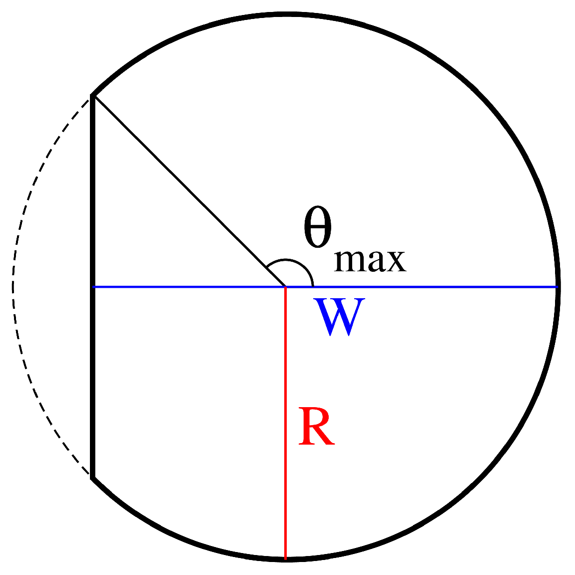
Figure 2.
Poincaré section is shown for 1 trajectory for time up to with the hard chaos case (left panel), and for 361 trajectories of 1000 points for each trajectory for the case of divided phase space with large integrable islands (right panel) with large integrable component. Here, are conjugate variables, where is the position at which the collision with the vertical line occurs. The term is the tangential component of the particle’s momentum, with being the angle of incidence in the collision.
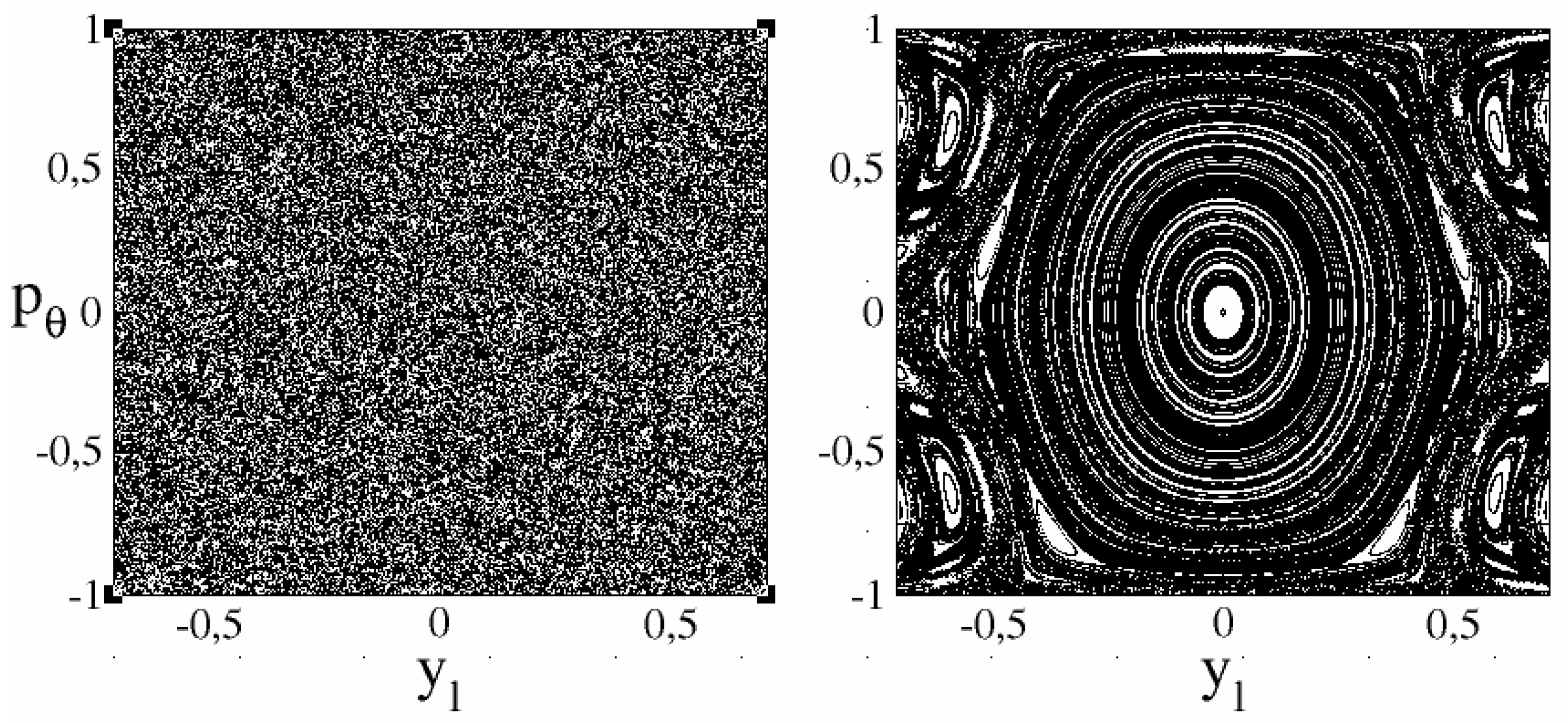
Figure 3.
Bottom panel shows first energy values for both parities with respect to the y-axis (odd and even); six top panels show the amplitude of real eigenfunctions for (marked by blue points of bottom energy panel). The color scale of wave functions a includes negative values for and ranges from minimum (red) to maximum (yellow), passing through blue, light blue, and green. For at red corresponds to zero for the ground state () while light blue represents zero for the other states.
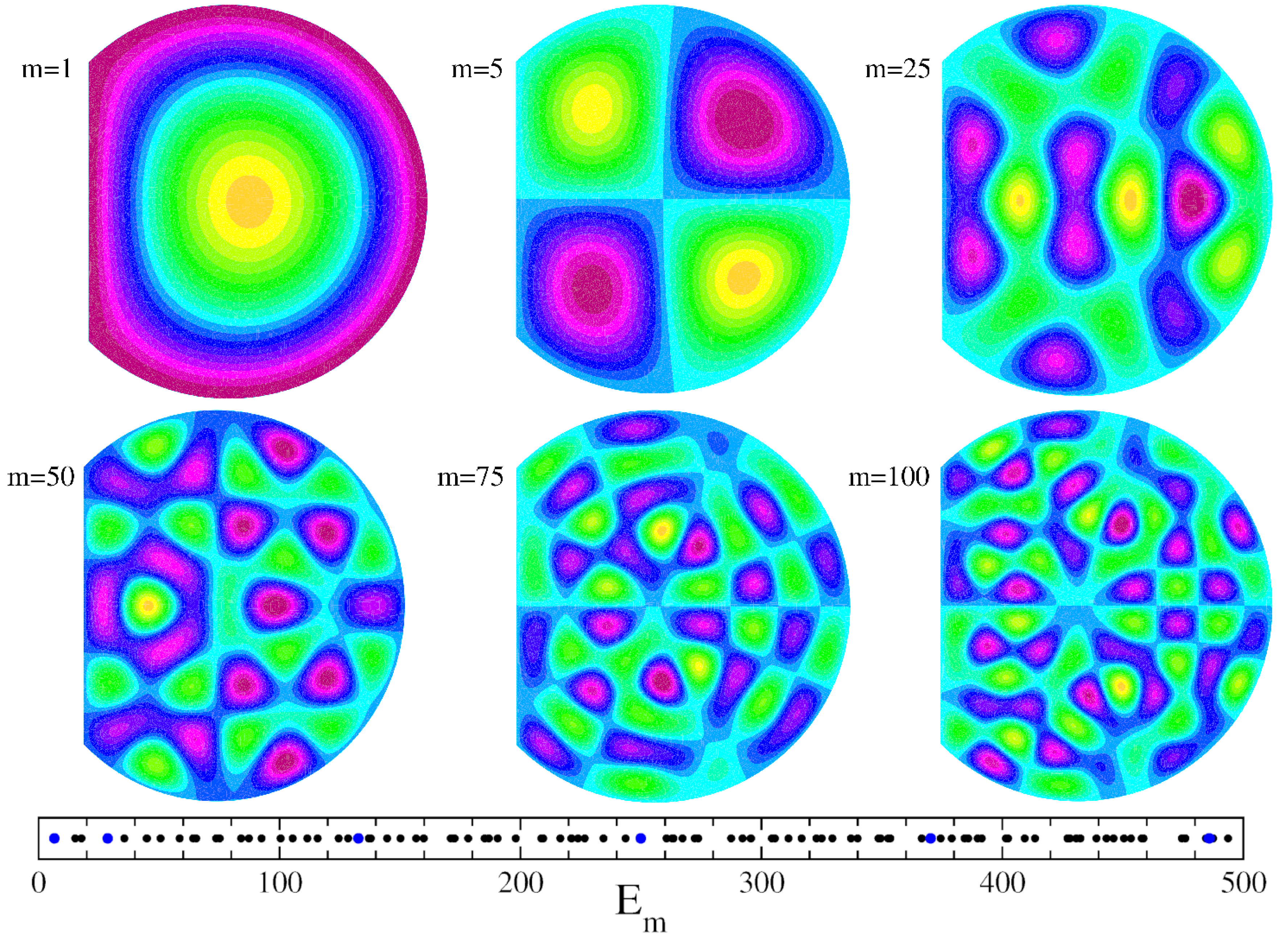
Figure 4.
Histogram for the level spacing statistical distribution is shown by blue and red bins for even and odd parity respectively. This distribution is calculated for both even and odd parity eigenstates. The theoretical Wigner surmise is shown by a full curve. Here, s is the energy level spacing rescaled by the average level spacing for fixed parity states. The histogram is obtained with the lowest 2000 energy levels.
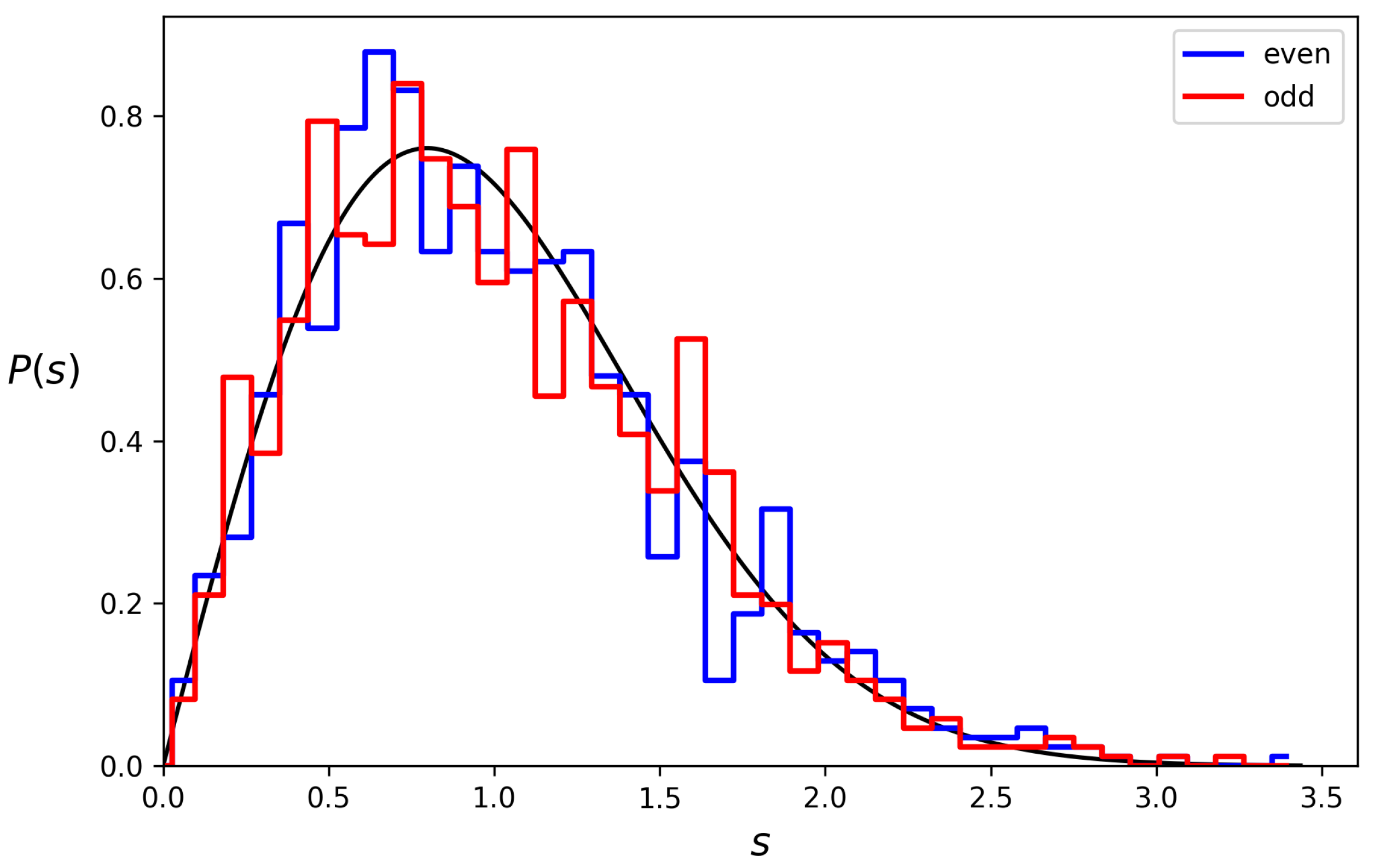
Figure 5.
Dependence of initially energy on total number of levels in the RJS model with , , for fixed probability of condensate at the ground state with .
Figure 5.
Dependence of initially energy on total number of levels in the RJS model with , , for fixed probability of condensate at the ground state with .
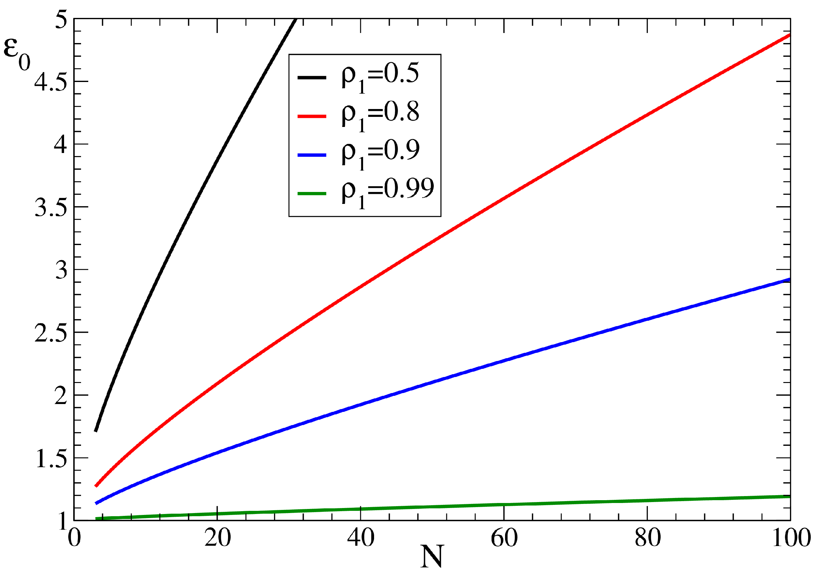
Figure 6.
Color map of condensate probability at corresponding system temperature T and number of system modes N (left panel); right panel shows the same as in left panel but in the plane ; obtained in the frame of RJ thermal distribution (2).
Figure 6.
Color map of condensate probability at corresponding system temperature T and number of system modes N (left panel); right panel shows the same as in left panel but in the plane ; obtained in the frame of RJ thermal distribution (2).
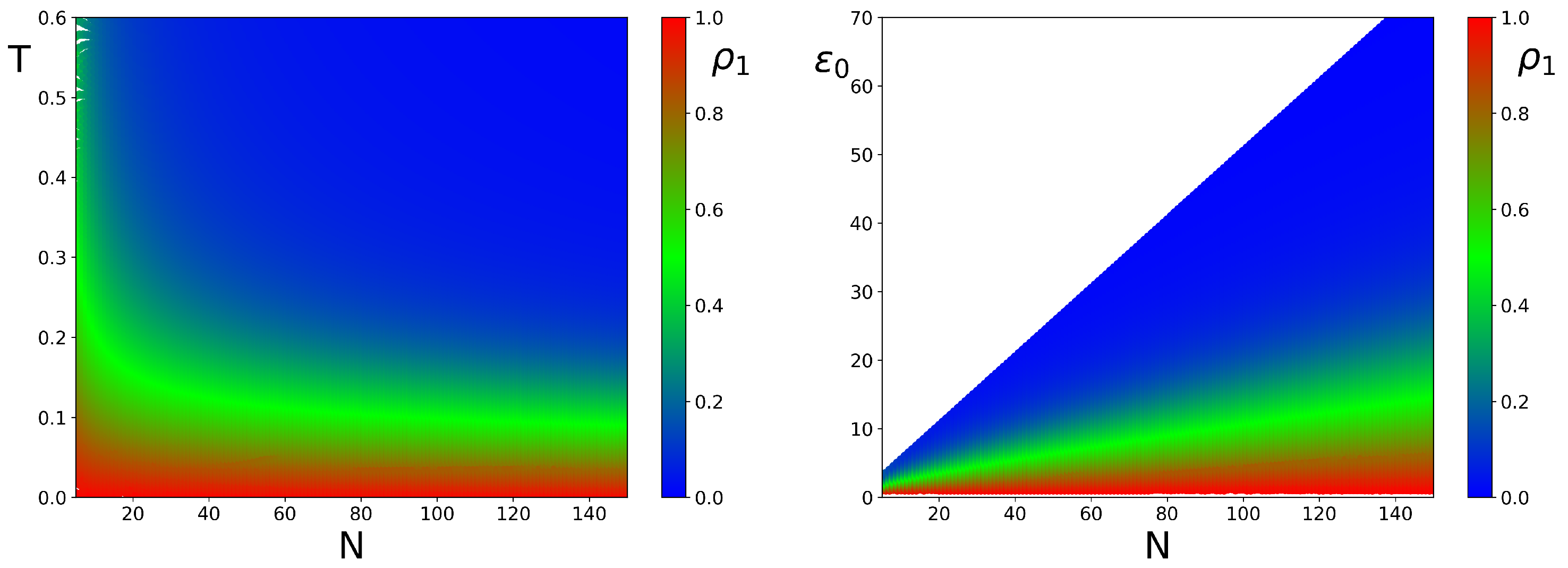
Figure 7.
Thermal RJ distribution (2) for various mode energies at and initial total energy ; ; data is presented in log-log scale.
Figure 7.
Thermal RJ distribution (2) for various mode energies at and initial total energy ; ; data is presented in log-log scale.
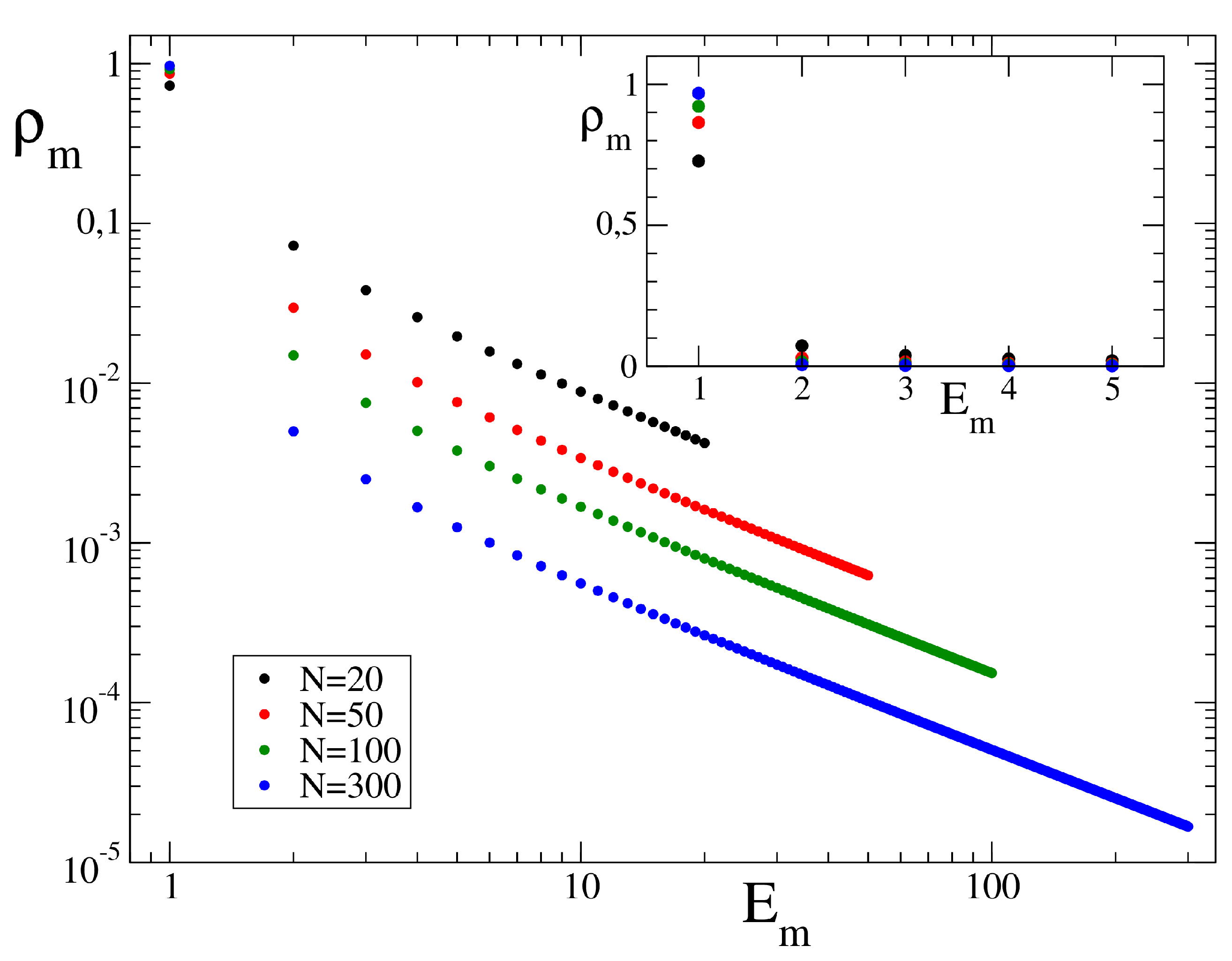
Figure 8.
Dependence of the non-condensate probability, , on the total number of modes, N, at a fixed total energy of . Here, represents the ground state population. The dashed curve shows the analytical theory given by the average Gumbel distribution with , for where is the Euler-Mascheroni constant (see text).
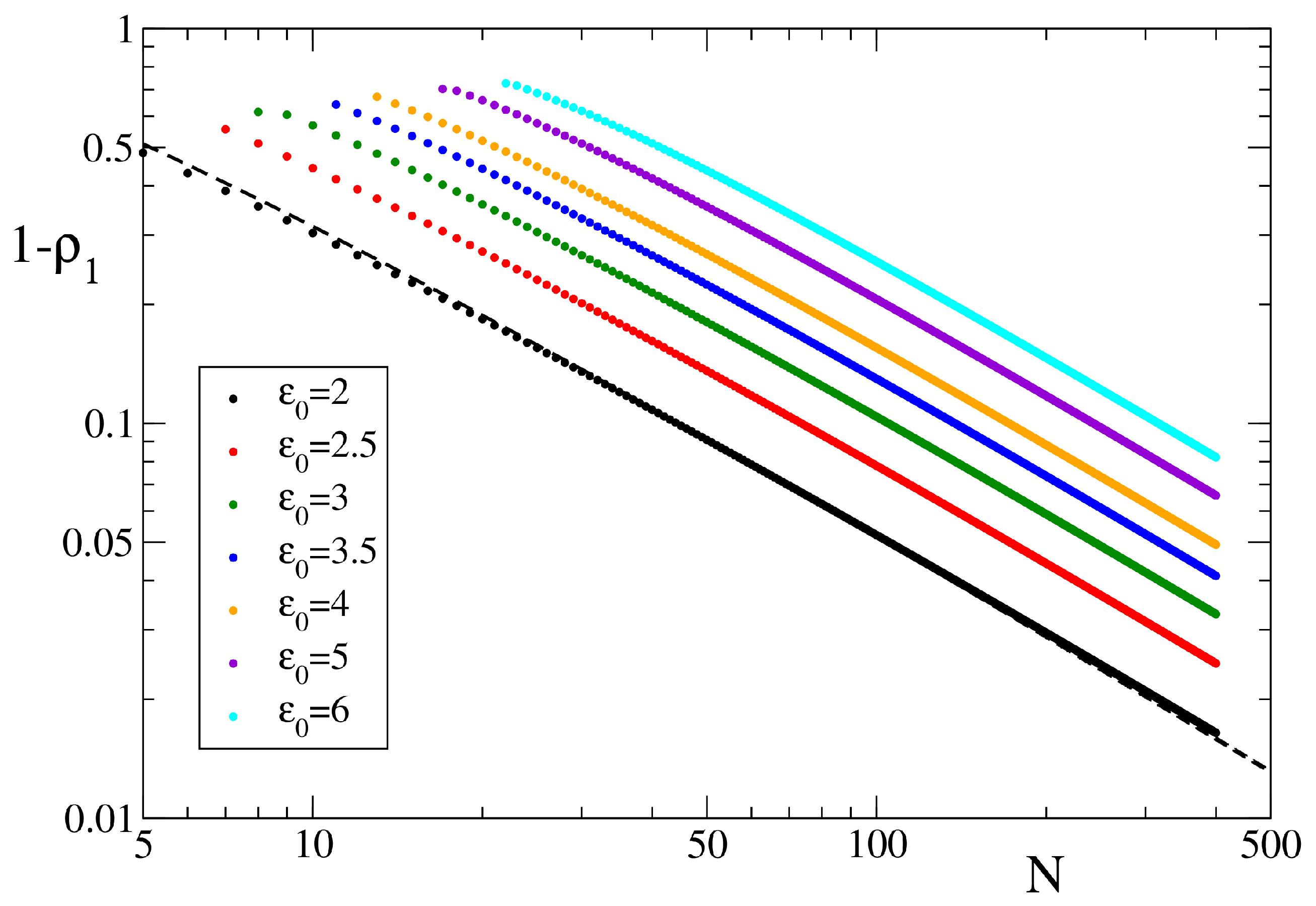
Figure 9.
Color plot of condensate probability . The left panels show plots of T vs. N, while the right panels show the distributions of vs. N. The top panels display the case of the D-shape billiard, with energies of the D-shape fiber described in Section 2. The bottom panels show the corresponding plots for the Sinai oscillator, with energies from [70].
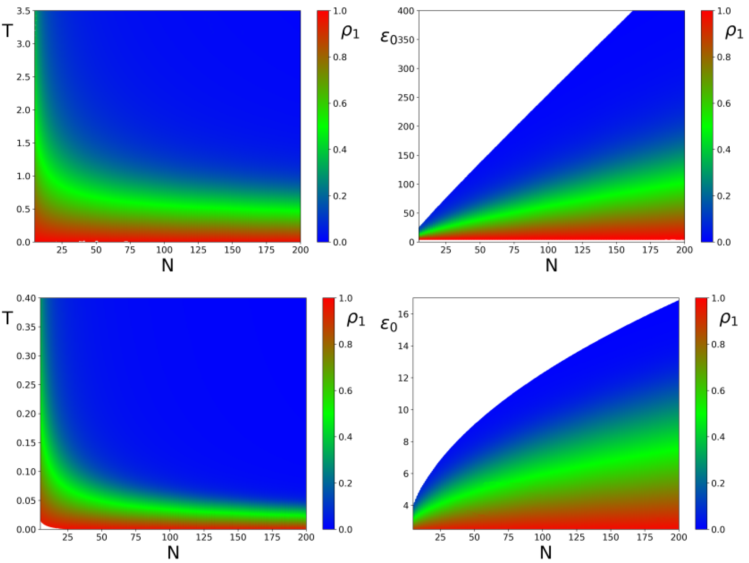
Figure 10.
Entropy (S) as a function of energy (E) for Bose-Einstein (BE) distributions (red solid line, Eq. 1) and Rayleigh-Jeans (RJ) distributions (blue dashed line, Eq. 2). The left panels show the simple model with equidistant energy levels, while the right panels are for energy states given by the D-billiard. The top panels show the case of states, and the bottom panels for states. For the D-shape billiard the lowest energies are .
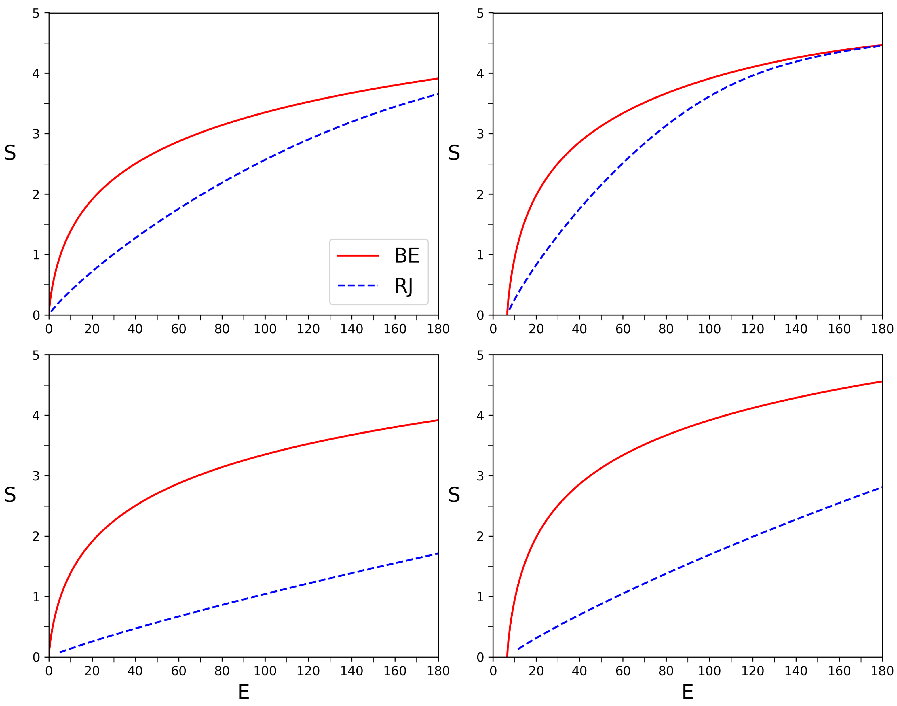
Figure 11.
Probability distribution for fluctuations of RJ condensate population at the ground state for the RJS model of N equidistant energy levels in RJ thermal distribution (2) with energy and norm conservation, comparing Monte Carlo simulations, exact analytical expression Eq. (13) and asymptotic Gumbel distribution Eq. (16).
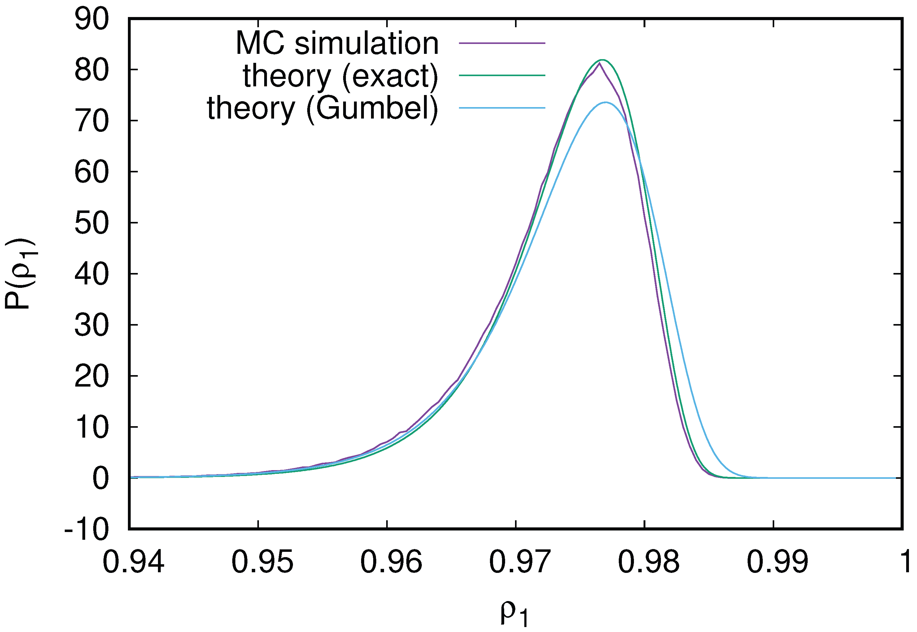
Figure 12.
Time dependence of the ground state probability shown up to for various initial states. The color of each curve corresponds to the initial total state energy, as indicated in the legend; the initial states are for (from minimal to maximal total energies E given in the figure panel); the plot shows a temporal average over time interval ; here . RJ and BE ansatz are shown for by the black and red dashed lines respectively for and ; the values of parameters obtained for both ansatz are , for RJ and , for BE.
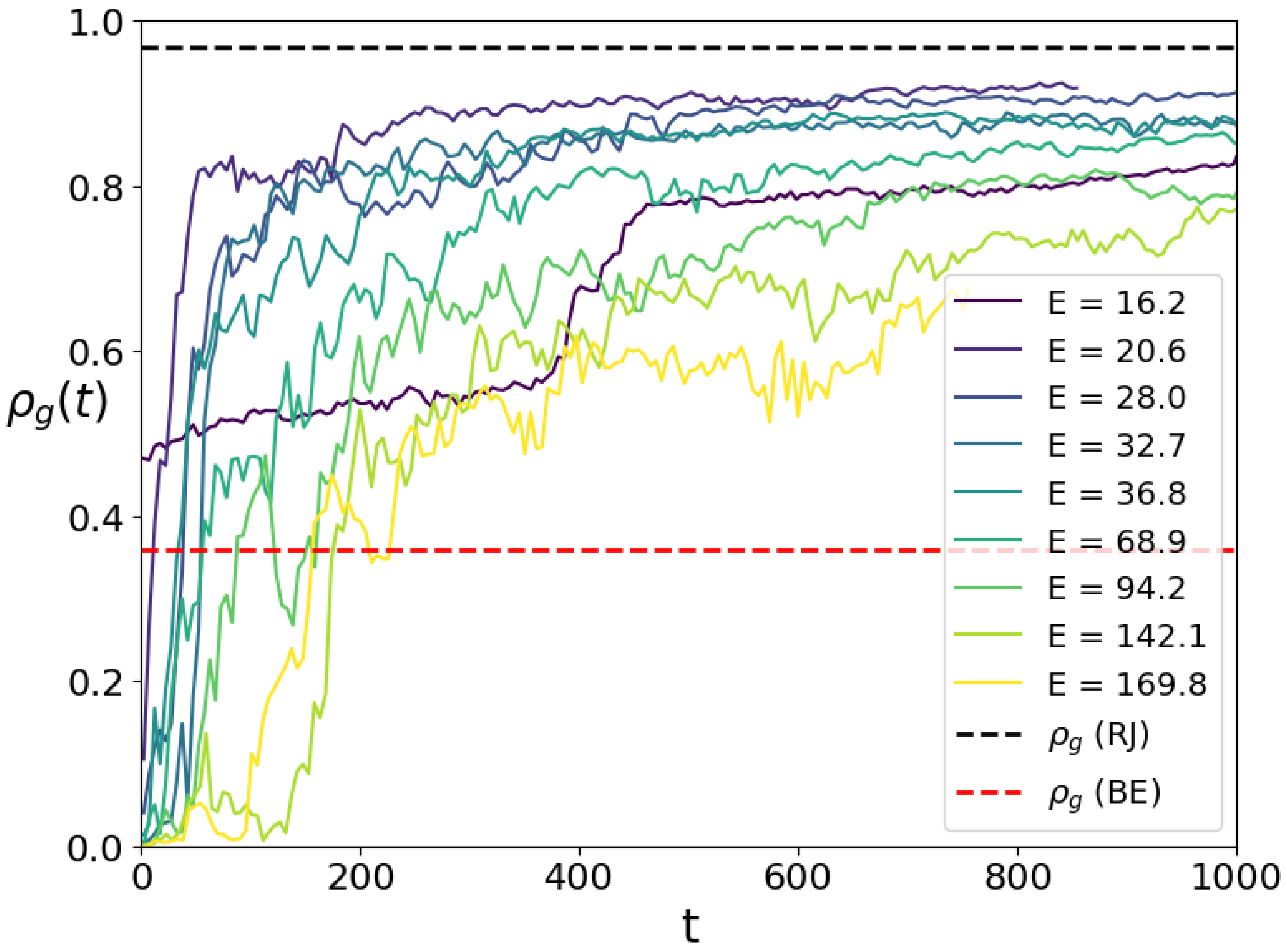
Figure 13.
Probability at eigenstates () as a function of linear eigenstate energy for different initial states and averaged over the time interval to ; other parameters are as in Figure 12. Colors correspond to the same initial states as in Figure 12; RJ and BE ansatz parameters are shown by dashed curves described in Figure 12.
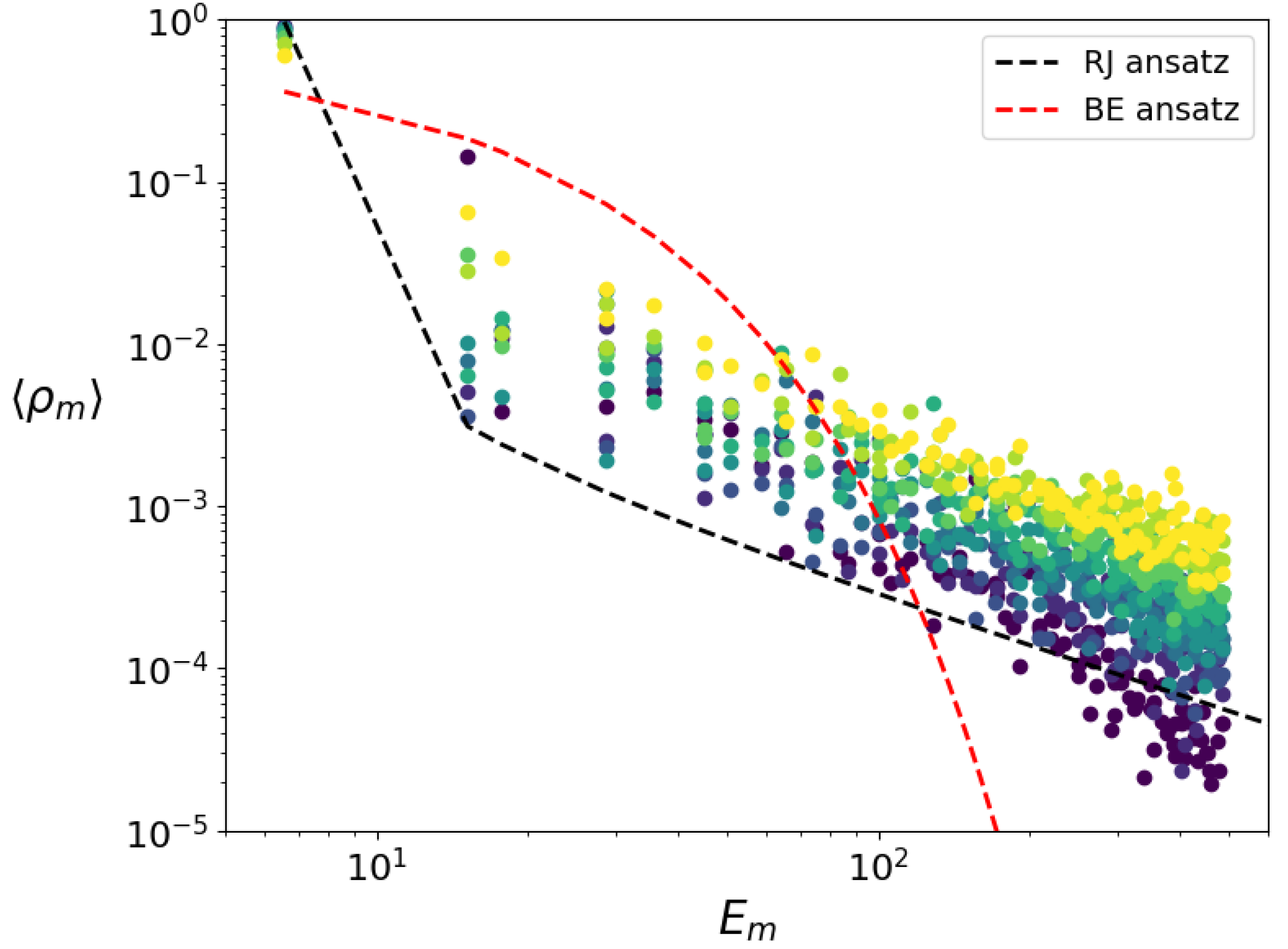
Figure 14.
Dependence of entropy S on time t for and other parameters as in Figure 12; values of S are averaged in the time window to reduce the fluctuations; short time behavior of is shown in Appendix Figure A2.
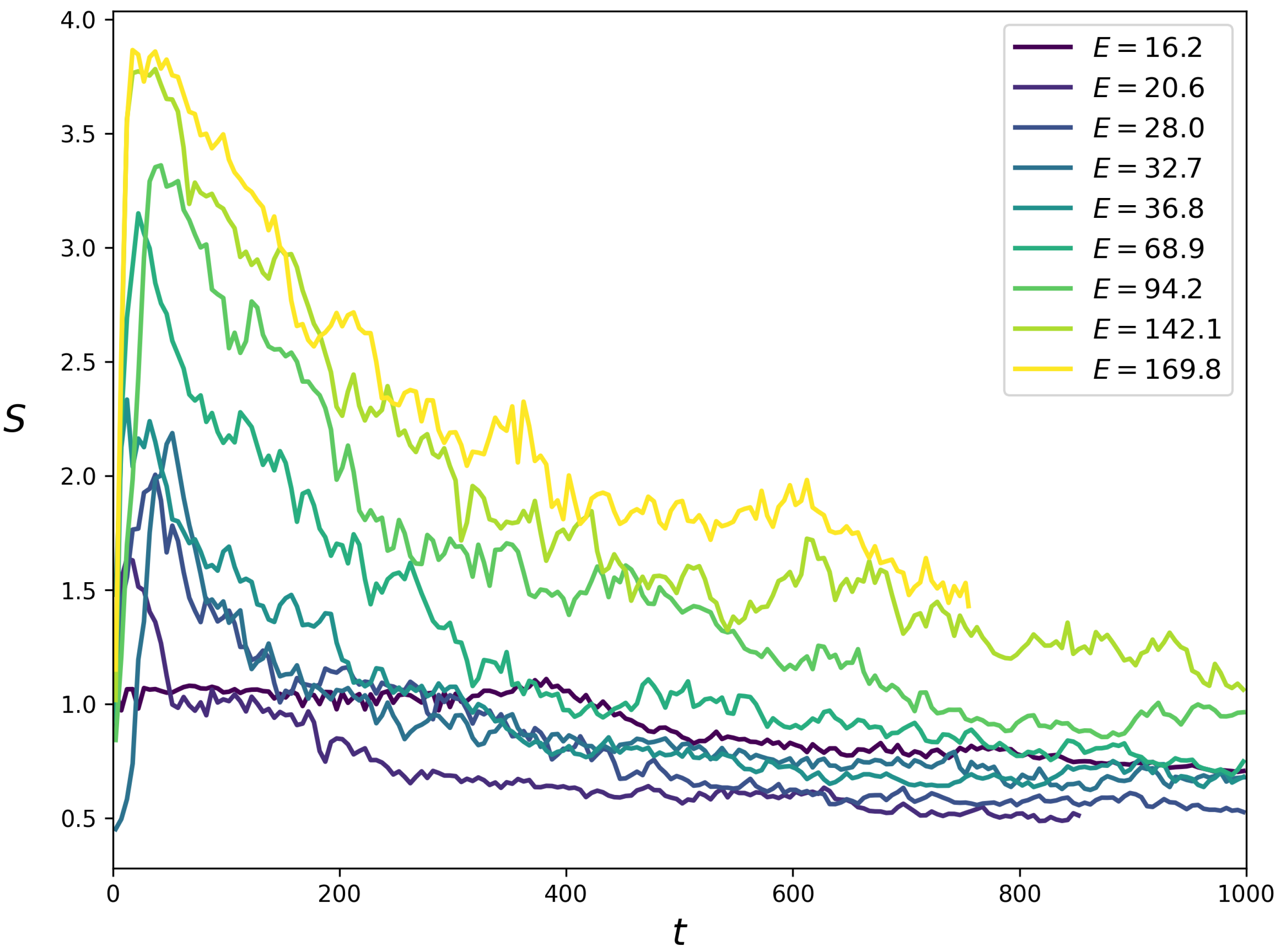
Figure 15.
Entropy S vs energy E are shown by points for the initial states of Figure 12 and Figure 13. The left panel displays the time average for times between 30 and 50, while the right panel shows the average for times between 500 and 1000; here as in Figure 12E is the total energy. In both panels, the curves are shown for the Bose-Einstein (BE) and Rayleigh-Jeans (RJ) distributions for the billiard with .
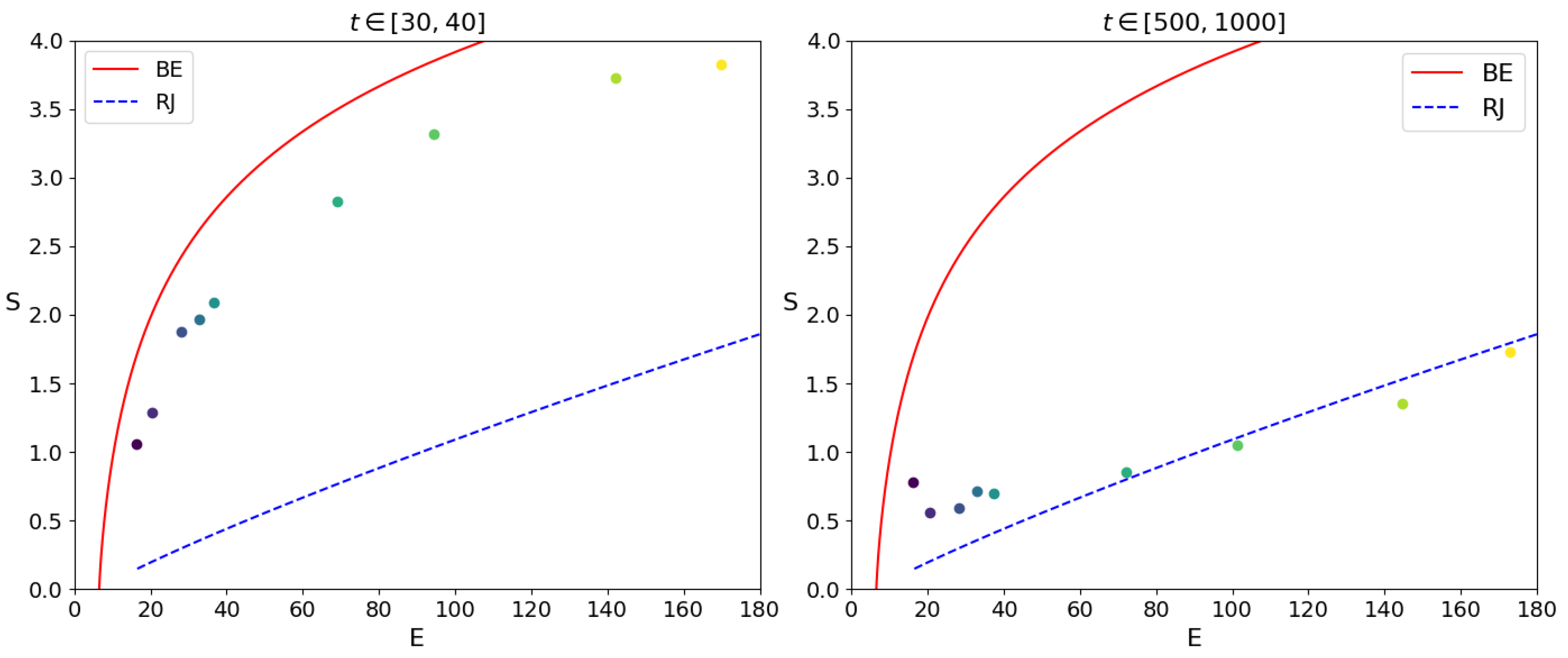
Figure 16.
Left panel: amplitude of wave function of the ground state at ; right panel: amplitude of the self-consistent solution of the NSE (3) at ; overlap probability between these states is . Amplitude is changing from zero (blue color) to high value (red color) and maximal value (light red in the center); wave functions are normalized to unity.
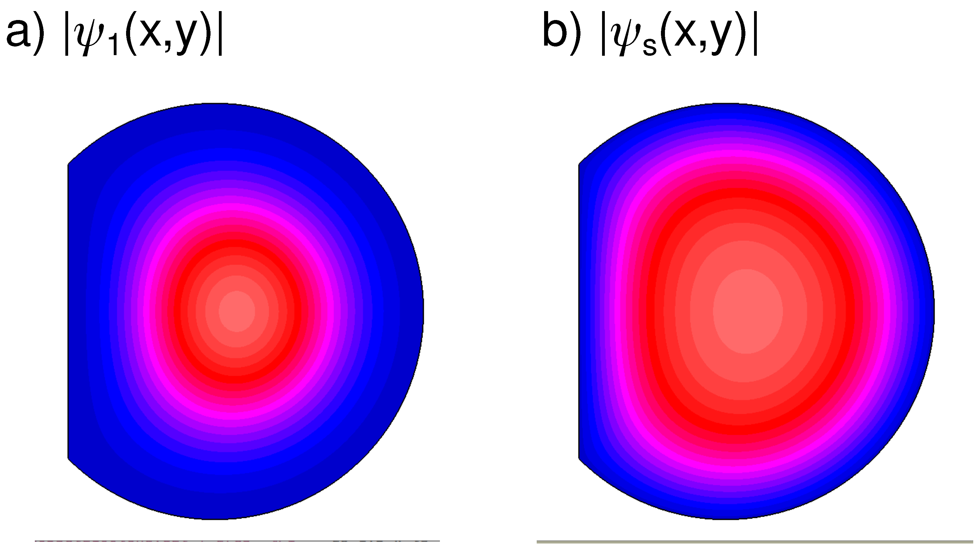
Figure 17.
Stability of self-consistent states obtained near the ground state and first excited state: the error of initial deviation remains approximately constant in time t showing that the state is table near a vicinity of the ground state while in a vicinity of the first excited state the error grows exponentially with time showing that the corresponding self-consistent state is unstable.
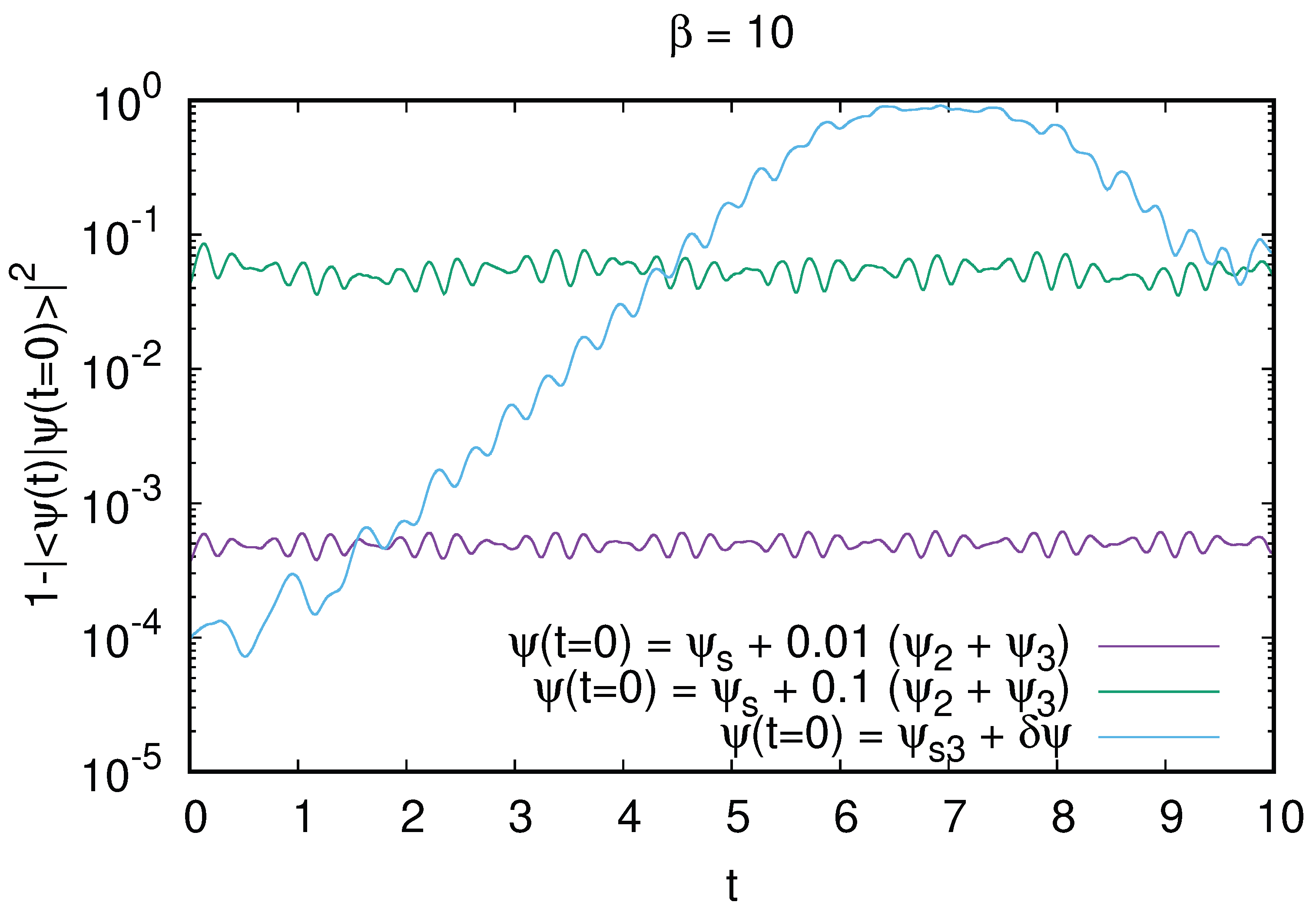
Figure 18.
Entropy S dependence on time for the initial state at and (values of S are averaged over a time window ).
Figure 18.
Entropy S dependence on time for the initial state at and (values of S are averaged over a time window ).
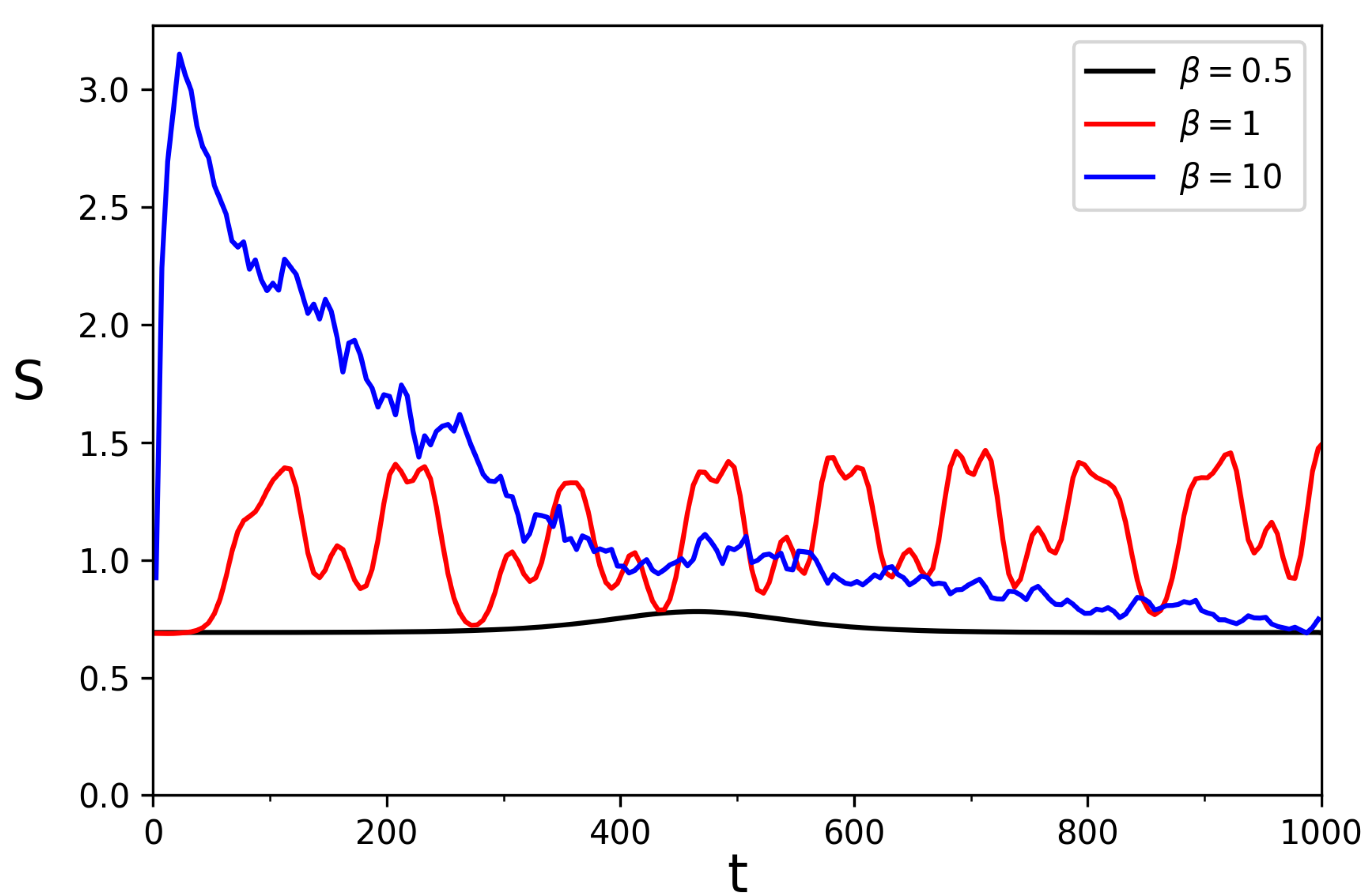
Figure 19.
Dependence of kinetic energy on time t in the NSE (3) at ; the initial state at is the linear ground state with the initial total energy (magenta curve), here the collapse takes place at with the divergence of ; the initial state is given by a linear combination of ground state and excited state at with , , and collapse happens at ; the initial state is taken as the first linear excited state at the initial total energy (green curve) for which there is no collapse and only oscillations of with time t. Here FREEFEM size is , integration time step , the relative accuracy of norm conservation is typically , with an increase up to maximal at specific time moments, and a relative accuracy of total energy conservation is typically with maximum being .
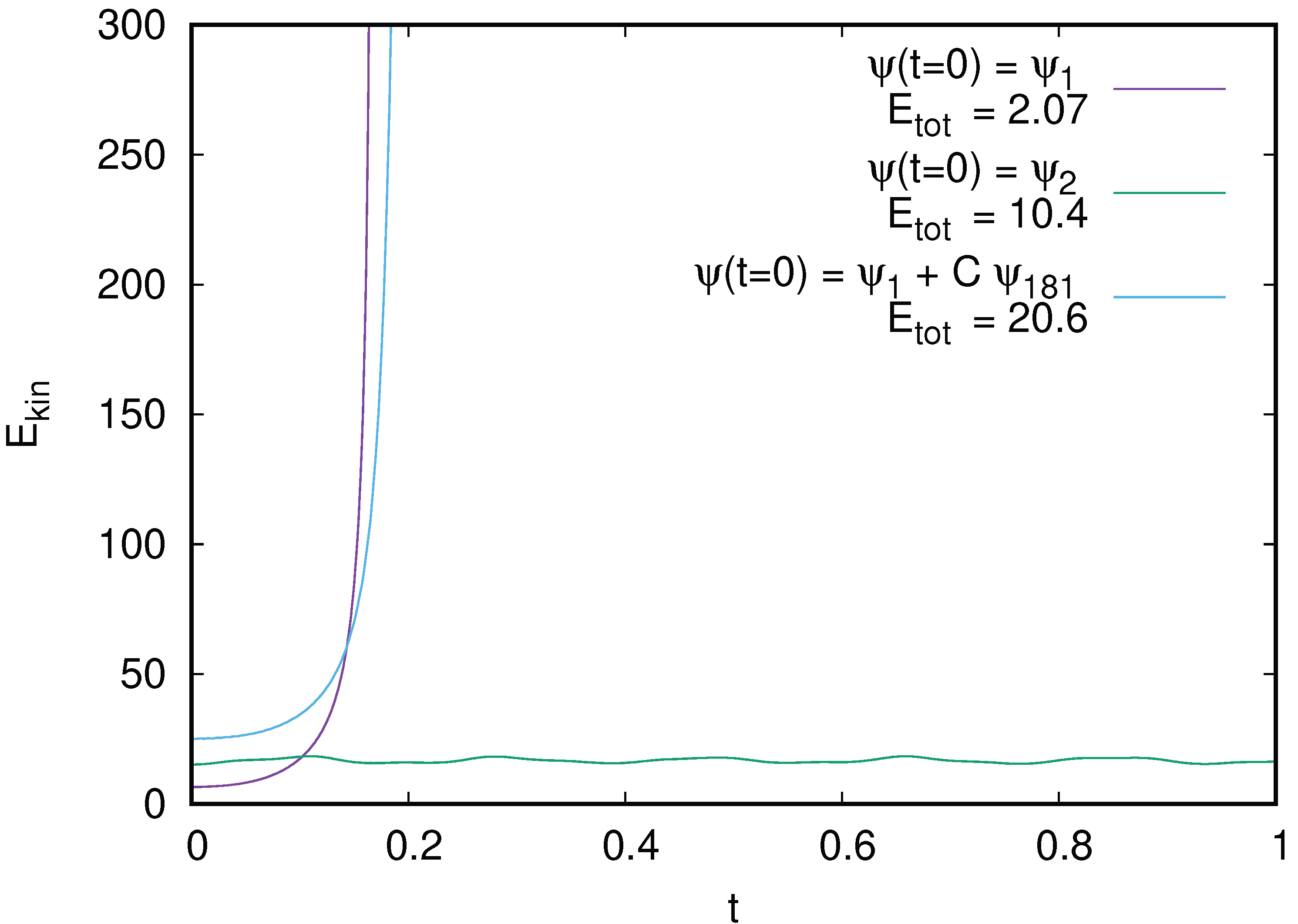
Figure 20.
Top panel: oscillating dependence of kinetic energy on time t (total energy is constant) for and the initial state is given by a linear combination of ground state and excited state at with and , , : no collapse (compare with collapse at in Figure 19). Bottom panel: for the case in the top panel we show the time dependence of the main part of probability in the eigenstates n of instantenious potential given by ; there are diabatic transitions between n-levels, shown by color bar, see text for details. Numerical integration parameters are as in Figure 19.
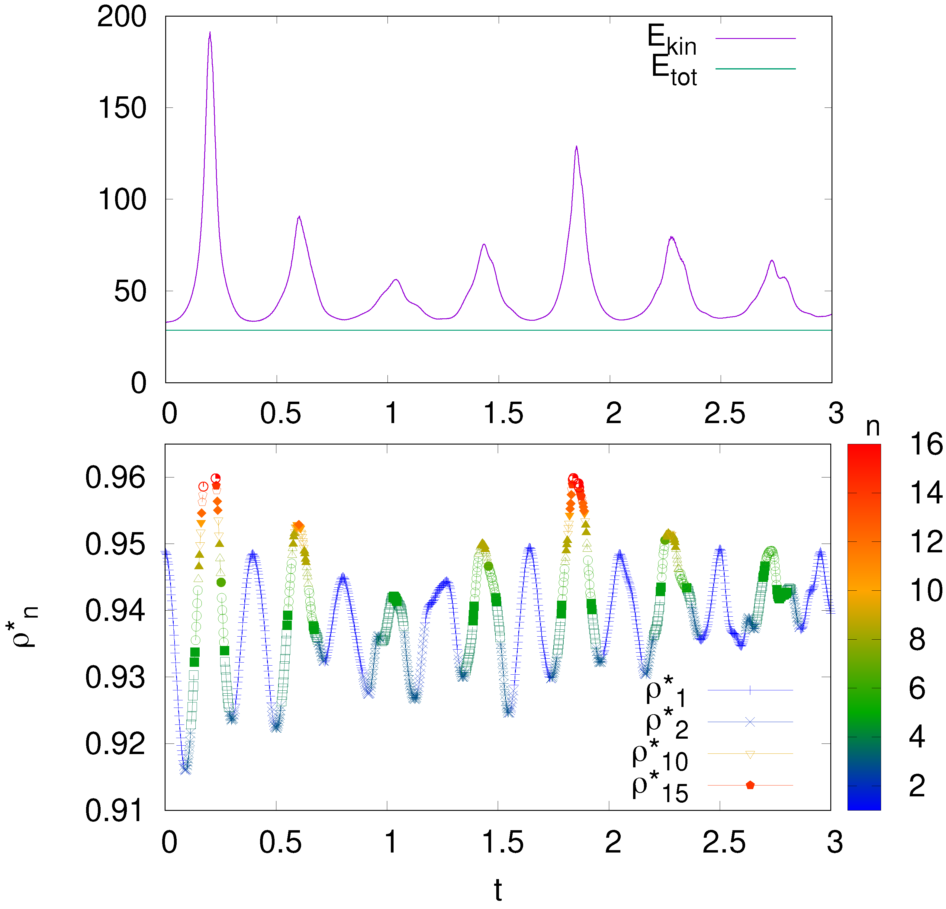
Figure 21.
Dependence of ground state probability on time t as in Figure 12 but for and only one initial state at ; the projection probability on the linear ground state is shown by blue curve and those on the ground state of instantaneous potential is shown by green curve; total energy is ; the dashed lines show BE ansatz (red) and RJ ansatz (black) with the same values of E, T, , N as in Figure 12.
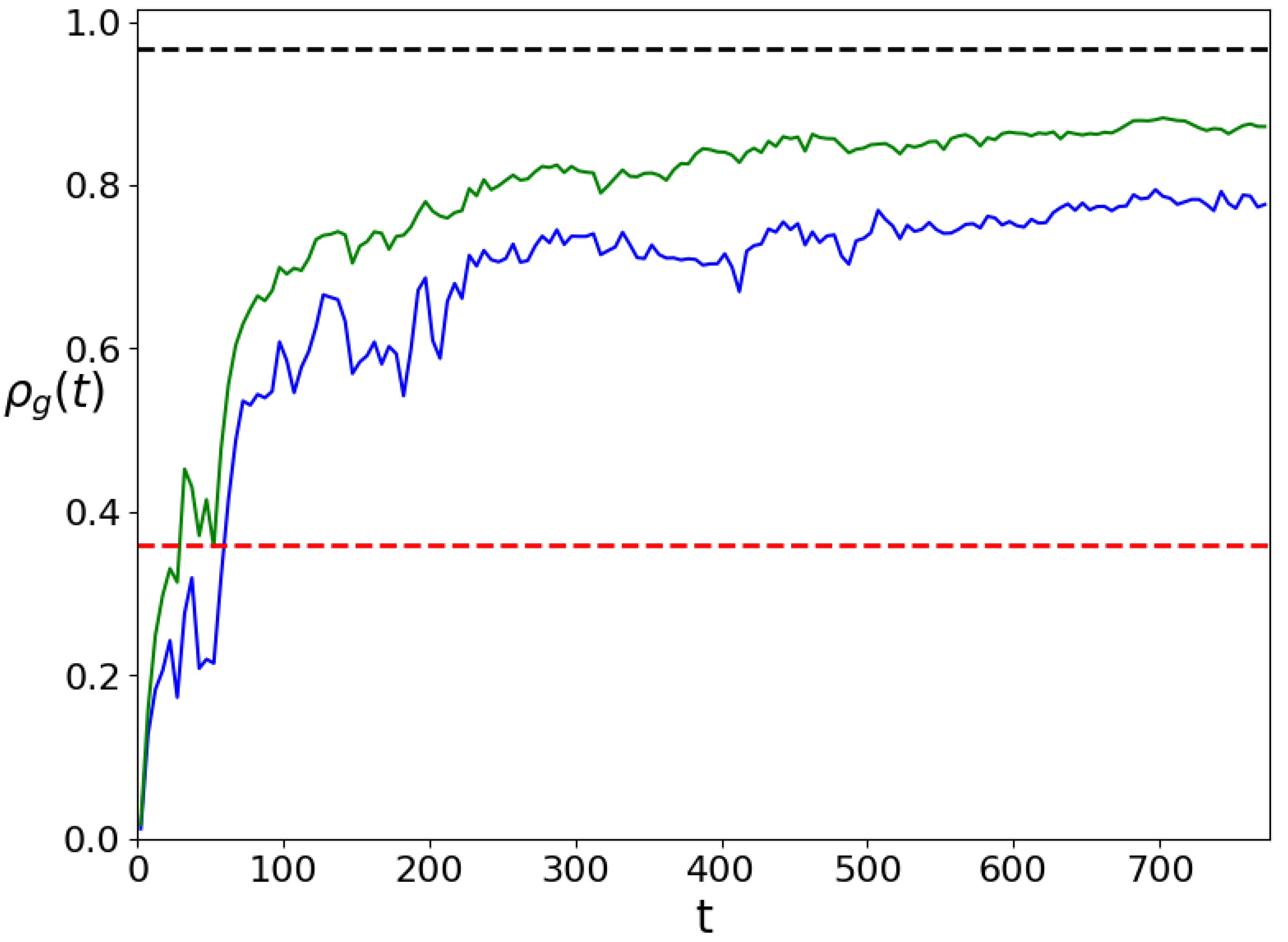
Figure 22.
Projected probabilities in the linear eigenstates and averaged in the time interval are shown in dependence on linear eigenenergies at and initial state as in Figure 21; dashed curves show the BE and RJ ansatz with same parameters as in Figure 12.
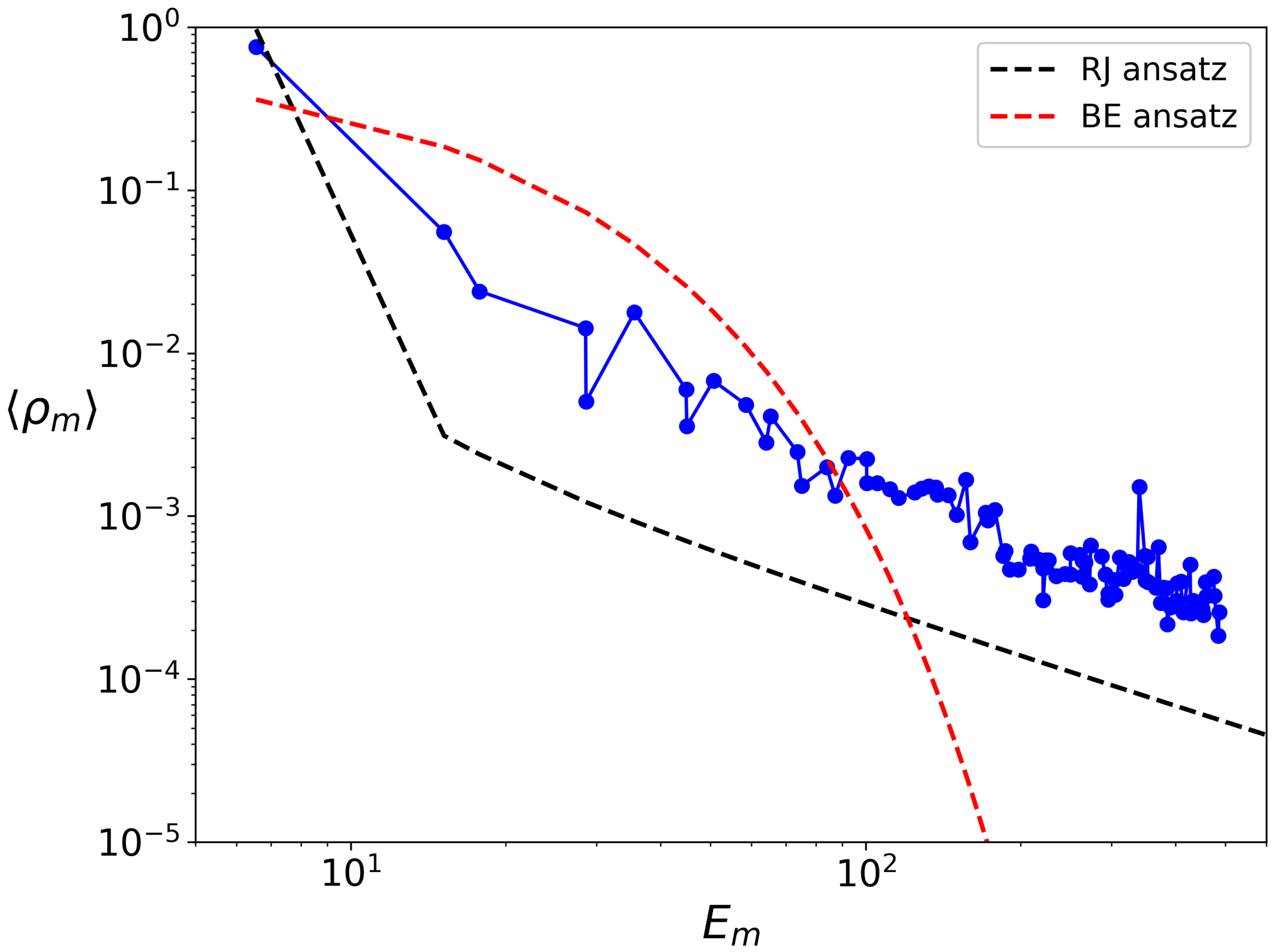
Figure 23.
Dependence of entropy on time t for (blue curve ) and (red curve) with initial state at ; left/right panels show long/short time behavior.
Figure 23.
Dependence of entropy on time t for (blue curve ) and (red curve) with initial state at ; left/right panels show long/short time behavior.
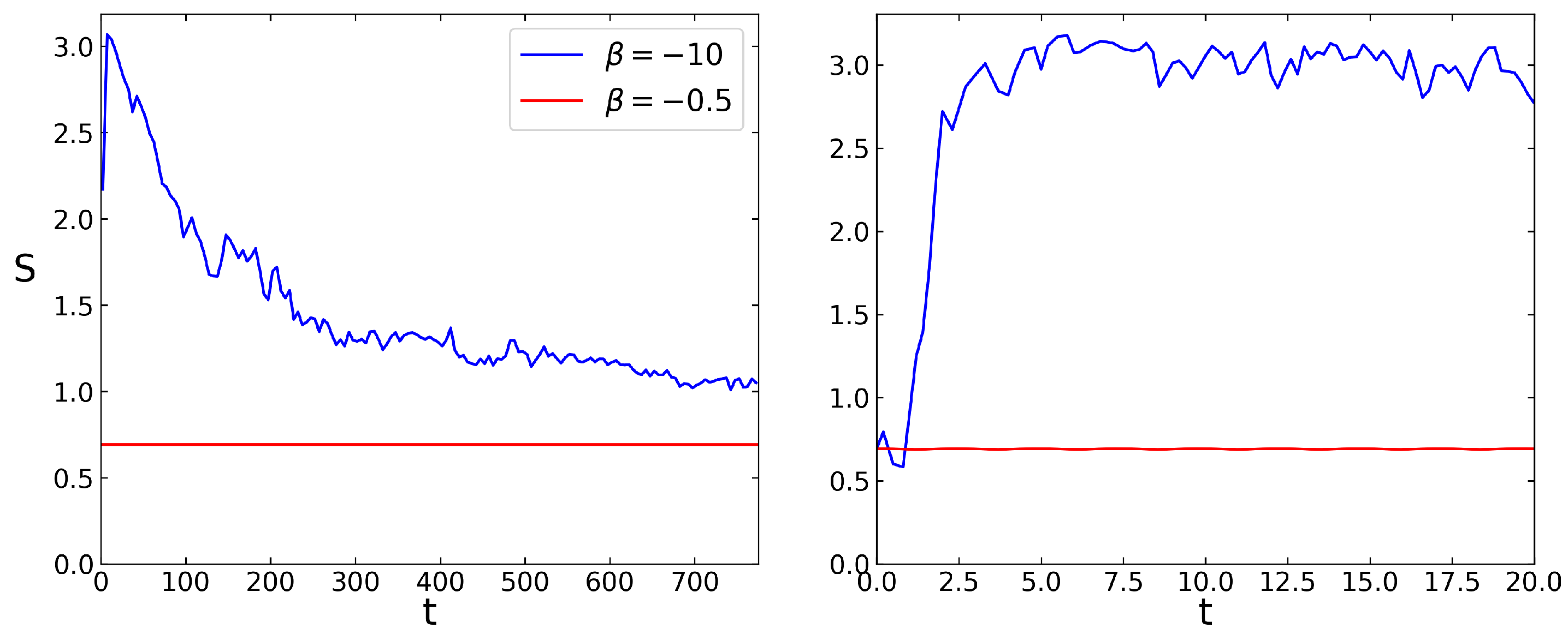
Figure 24.
Left panel: probability in the linear ground state and first excited state (which is relatively close to vortex) as function of time t for different integration steps and with the number of intergration net nodes and respectively at . Right panel: color panels show the wave function amplitude and its phase at different moments of time; color scale as in Figure 16.
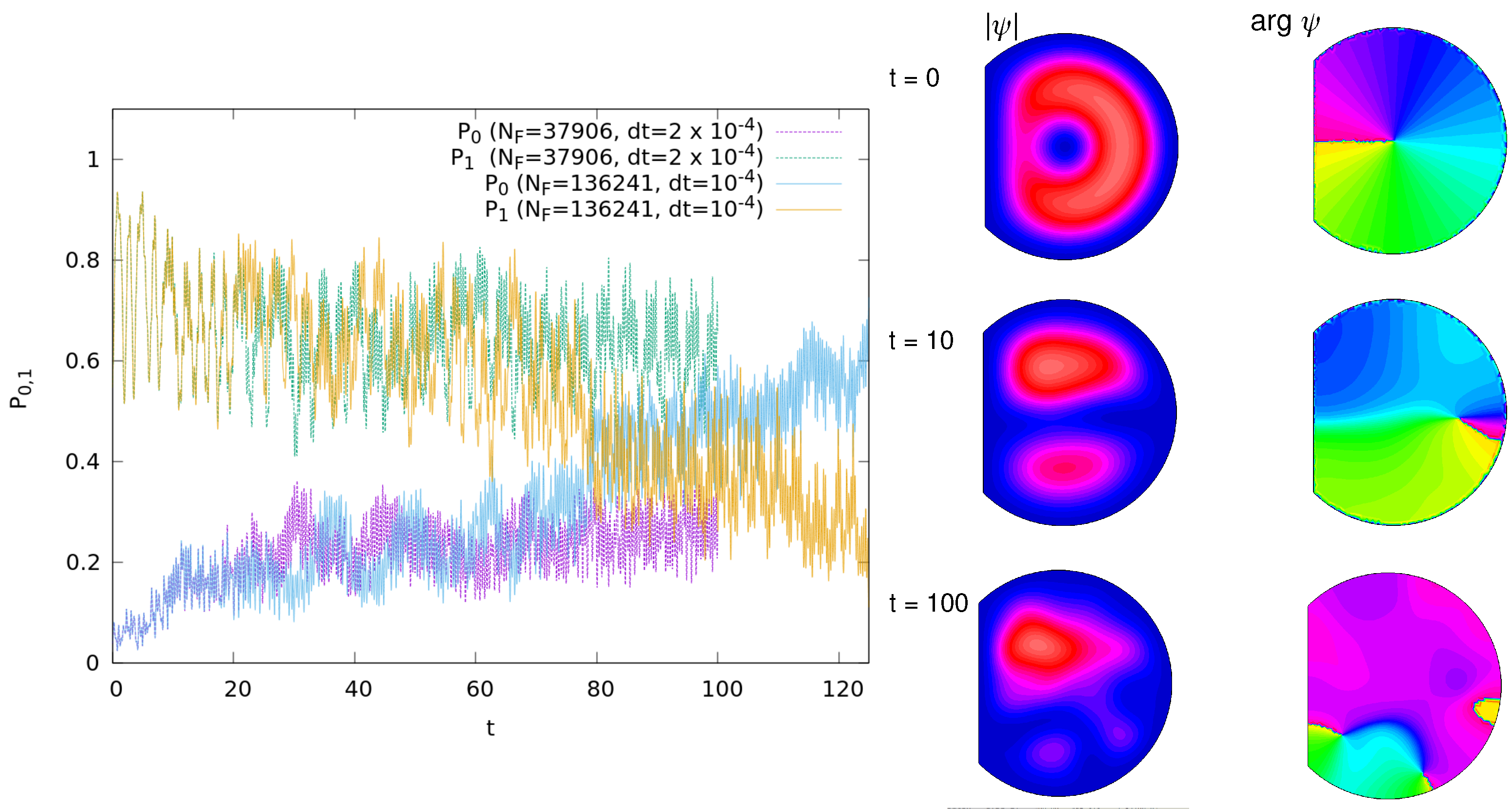
Figure 25.
Probability in the first linear excited state (close to vortex) as function of time t for different values; there is a sharp disapperance of vortex for ; for the same behavior continues up to and may be continued beyond this maximal computation time.
Figure 25.
Probability in the first linear excited state (close to vortex) as function of time t for different values; there is a sharp disapperance of vortex for ; for the same behavior continues up to and may be continued beyond this maximal computation time.
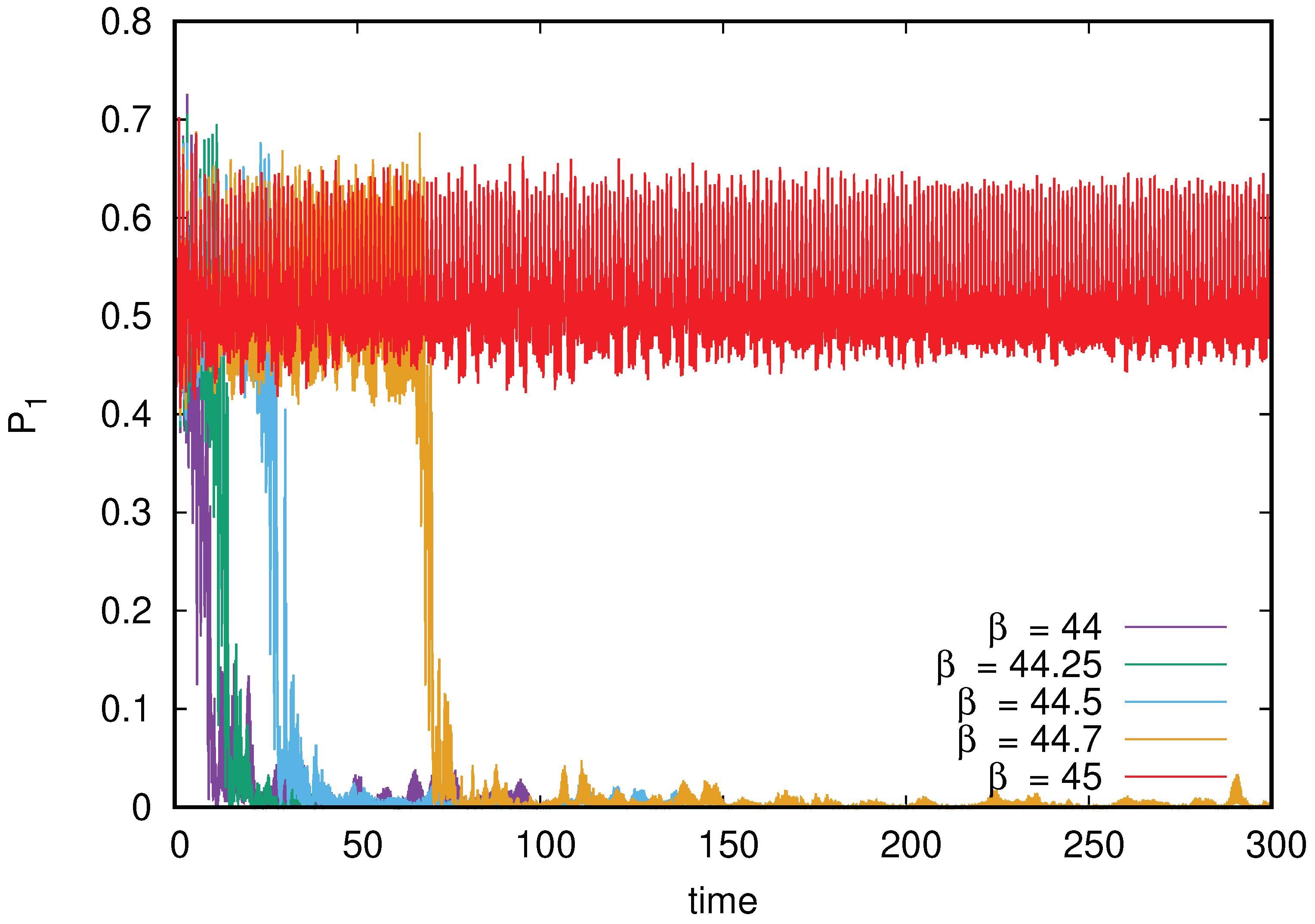
Figure 26.
Nonlinear vortex fields (amplitude and phase) are shown at time for (vortex is destroyed) and (vortex survive). The video of time evolution of is shown for (left image) and (right image) up to in the Supplementary Material file videovortex.mp4.
Figure 26.
Nonlinear vortex fields (amplitude and phase) are shown at time for (vortex is destroyed) and (vortex survive). The video of time evolution of is shown for (left image) and (right image) up to in the Supplementary Material file videovortex.mp4.
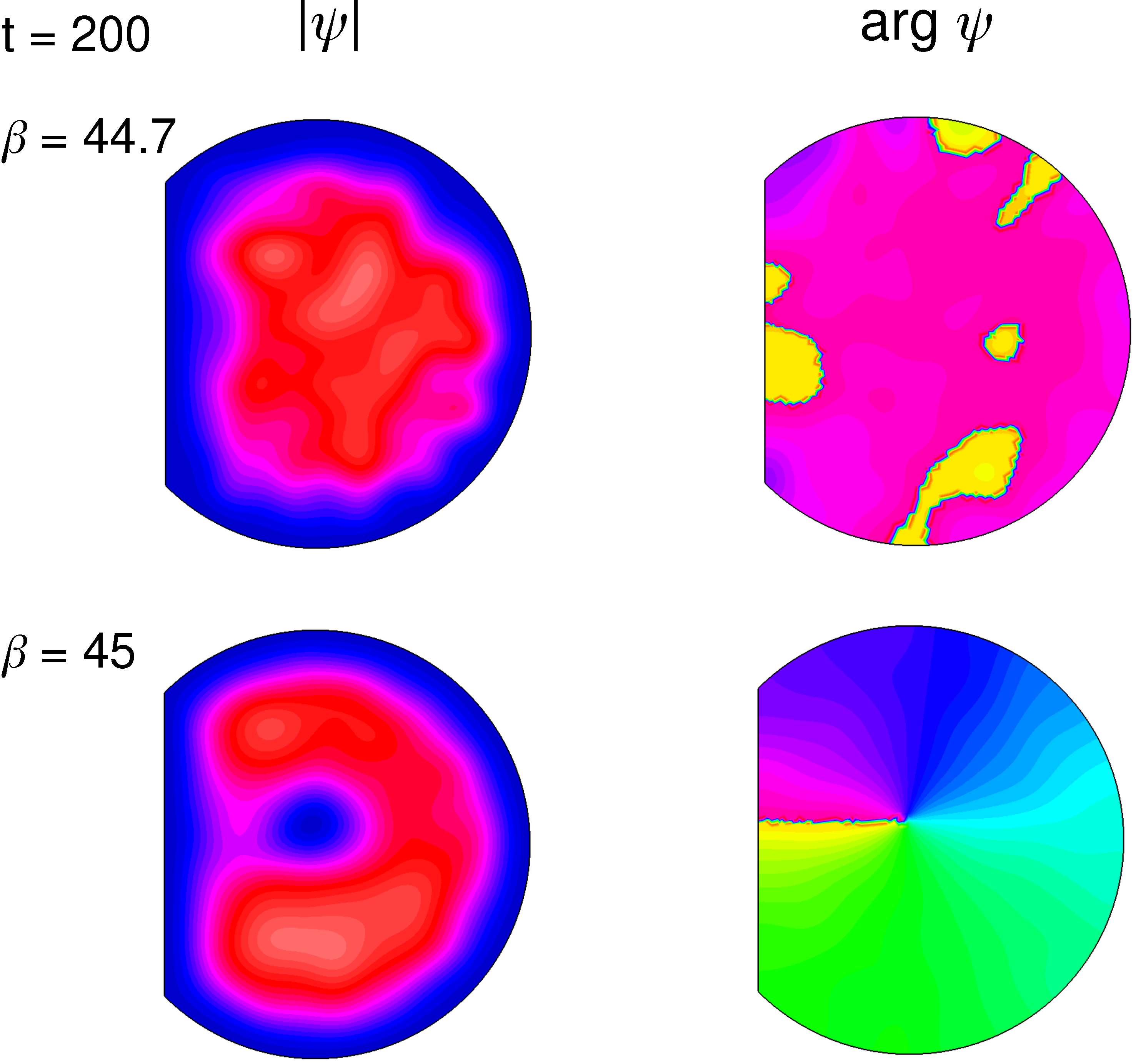
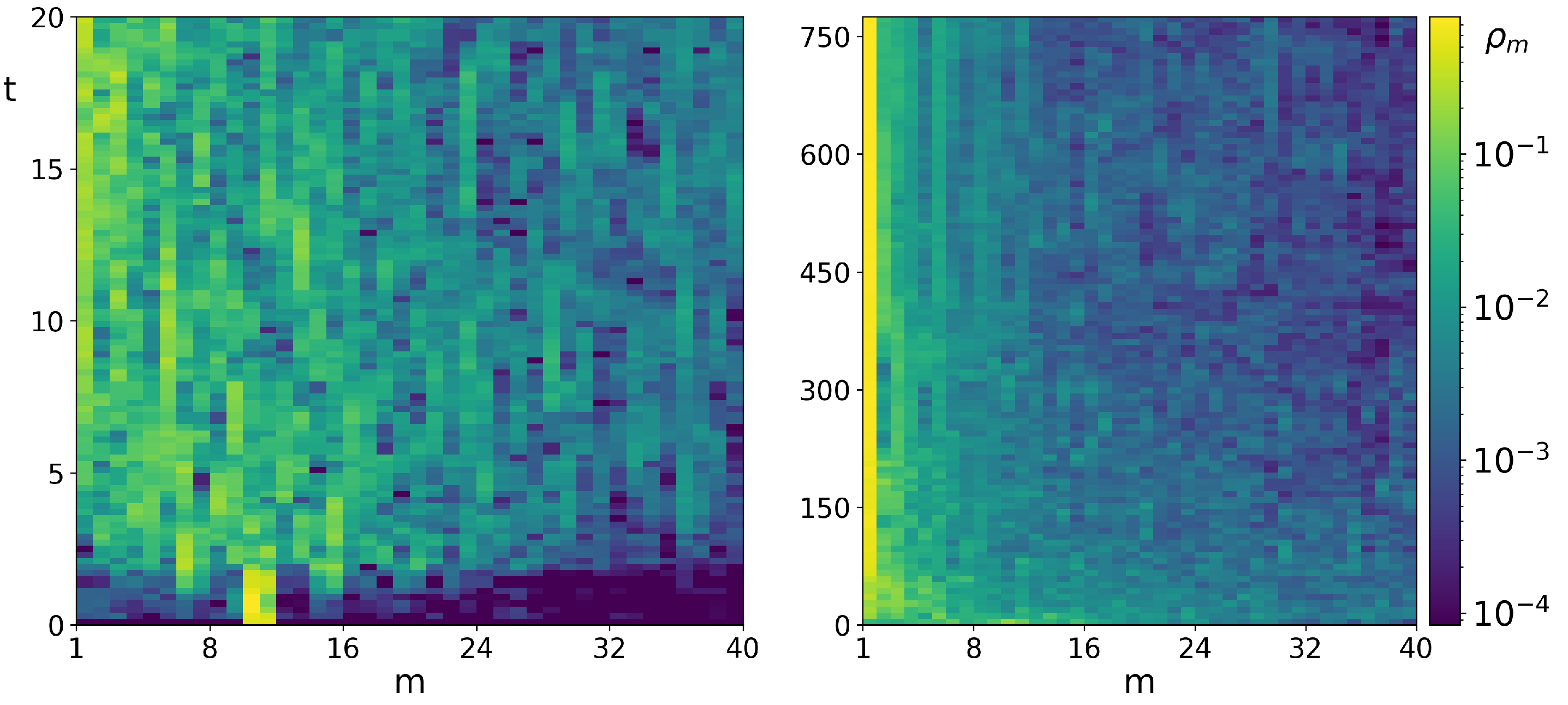
Disclaimer/Publisher’s Note: The statements, opinions and data contained in all publications are solely those of the individual author(s) and contributor(s) and not of MDPI and/or the editor(s). MDPI and/or the editor(s) disclaim responsibility for any injury to people or property resulting from any ideas, methods, instructions or products referred to in the content. |
© 2025 by the authors. Licensee MDPI, Basel, Switzerland. This article is an open access article distributed under the terms and conditions of the Creative Commons Attribution (CC BY) license (http://creativecommons.org/licenses/by/4.0/).
Copyright: This open access article is published under a Creative Commons CC BY 4.0 license, which permit the free download, distribution, and reuse, provided that the author and preprint are cited in any reuse.


