Submitted:
06 June 2025
Posted:
09 June 2025
You are already at the latest version
Abstract
In this paper we have introduced a new matrix and developed two algorithms to generate line graphs of undirected and directed graphs (digraph). The algorithms are tested for a large number of random graphs and the outputs are appended at the end of the paper. It has been found that the actual computing time is nearly 1% of the theoretical bound O(n4) of the algorithms.
Keywords:
Adjacency matrix
; incidence matrix
; line graph
; time complexity of algorithm
MSC: 05C85
1. Introduction
Let G(V,E) be a simple undirected graph where V = {vi | i= 1,2,…,n } is the set of vertices and E ={ ei | i= 1,2,…,m } the set of edges in G[West, 2000]. The line graph of G, denoted by L(G), is defined by a simple undirected graph with m vertices and q = -m + ( ∑ di 2)/2 edges where di denotes the degree of the vertex vi . The vertices in L(G) correspond to the edges in G, and two vertices in L(G) are adjacent if the corresponding edges in G have a vertex in common. If B is the incidence matrix of G, it is known that the adjacency matrix of L(G) is BTB (modulo 2) and the time complexity of computing L(G) by this result is O(n5) [ Harary, 1994].
Line graph of a graph was independently discovered by many authors. Whitney was the first, but he did not assign any name to it. But others gave it different names. Hoffman: line graphs; Beineke: derived ; Kasteleyn : covering; Menon : adjoint. Ore: interchange graphs; Sabidussi: derivative; Seshu and Reed: edge-to-vertex. Line graphs have lots of applications in electrical engineering [ Harary, 1994], in communication networks [Krawczyk M et al, 2011], in ‘characterization of DNA sequences’ [ Kumar. V, 2010], in ‘Codes and designs’ [Fish.W et al, 2011] in VLSI design [Tatsuo.O et al, 1979], to mention a few.
In this paper a new matrix called degree edge matrix of an undirected graph G has been used as a data structure to develop an efficient algorithm to generate L(G) from G. An analogous development for generating line graph of a digraph has also been done. The computing time of the algorithms for generating line graphs of undirected graphs as well as directed graphs is O(n4) [Chartrand. and Oellermann, 1993]. Both the algorithms have been coded to C programming [ ] and tested for a large number of random graphs with varying densities. When the programs are run for undirected as well as directed graphs, it has been found that the actual computing time in both the cases is nearly 1% of the theoretical bound O(n4).
In section 2, we have given relevant definitions with illustrations. In section 3, a new method is developed with a new matrix to generate line graphs undirected graphs. In section 4, we have suggested how we can minimize actual computing time. An algorithm for generating line graph of an undirected graph is developed in this section. In section 5, an analogous development for generating line graph of a digraph is given. Programmers in C corresponding to these two algorithms are written and tested for random graphs with varying densities. Finally, the outputs are appended at the end of the paper.
2. Definitions:
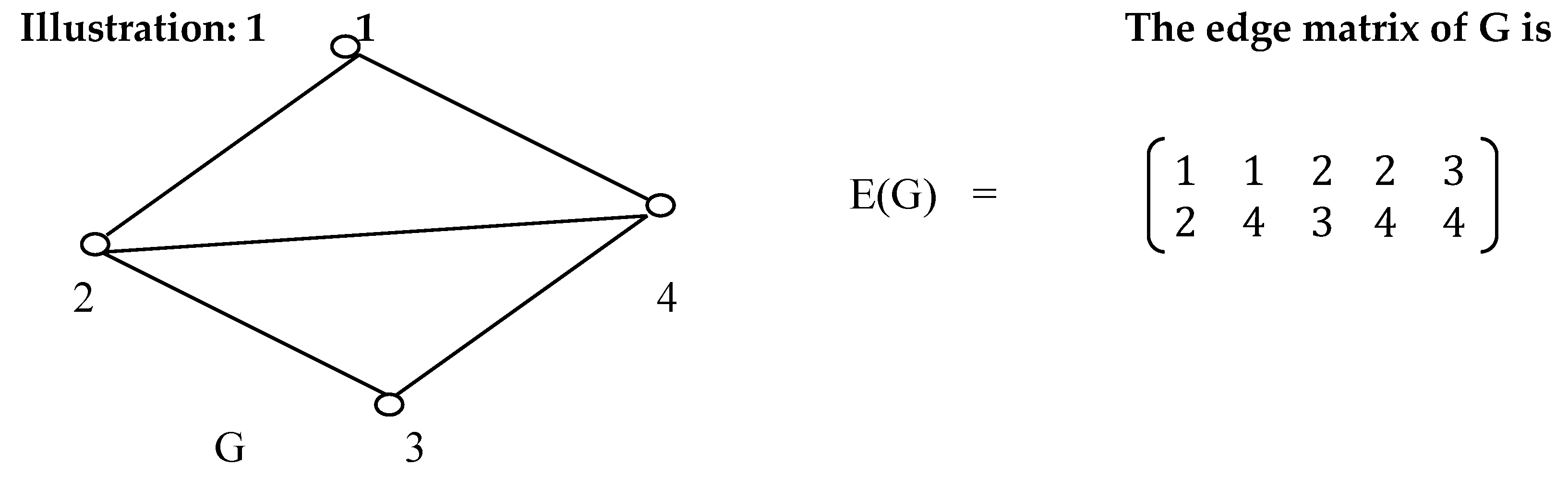
Definition1. The edge matrix of G (n,m), denoted by E (G), is a ( 2 x m ) matrix defined by
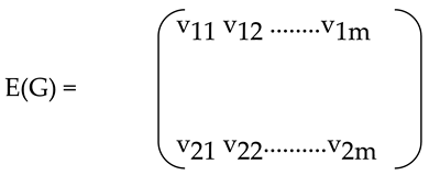
where a column represents two end vertices of an edge of G.
The vertices of G are renamed as vij and the edges as (v1j,v2j) for ( i= 1,2; j= 1,2,...,m).
Obviously, for a graph without self loops v1j v2j, j= 1,2 ... , m
and without parallel edges , iSince G is undirected, without any loss of generality we can choose the end vertices of the edges ej as v1j < v2j for 1≤ j ≤ m.
Thus if we compare any two columns (say j the and k th) of E(G), then two possible cases may arise:
(a) ej = and ek = have one vertex in common
(b) ej = and ek = have no vertex in common
Thus the adjacency between the edges of G can be studied with the help of the edge matrix of the graph.
Definition 2. The degree of an edge e = (u,v), denoted by d(e), is defined by
d(e) = d(u) + d(v) - 2.
Definition 3. The degree edge matrix of G (n,m), denoted by DE(G), is a (3 x m) matrix defined by
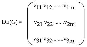
where the submatrix formed by the first two rows of DE(G) is the matrix E(G) and v3j is the degree of the edge ej for j = 1,2,..,m . The third row of DE(G) will be called the degree edge vector of G. In an analogous way we can define the matrices EL(G) and DEL(G) as the Edge Matrix and Degree Edge Matrix respectively of L(G).
3. A New Method to Generate Line Graph of an Undirected Graph
We now present a new method based on the edge matrix of a graph G as data structure to generate line graph of an undirected graph. To explain the method we consider the following examples.
Here the number of edges is 5 and the degrees of the vertices are 2, 3, 2, and 3.
So the number of columns of EL(G) is q= -5 + ( 4+9+4+9)/2 = 8.
From the 1st and 2nd columns of E(G), we see e1 and e2 are adjacent, hence they will be the
vertices of L( G). So the 1st column of EL(G) is (for convenience writing i for ei etc.)
Again, the lst and the 3rd columns of E(G) have an element (viz.2) in common,
the 2nd column of EL(G) will be Following this way we get the edge matrix of the line graph of G as
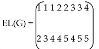
Since E(G) completely characterizes G, EL(G) does the same for L(G). The method of constructing EL(G) from E(G) as mentioned above is better than the existing method because the time complexity for computing EL(G) from E(G) is O(n4). This is due to the fact that the number of times the inner loop executed in the worst case is
(m-1)+(m-2)+ … +2+1= m(m-1)/2= O(m2) = O(n4).
4. Improvement of Actual Computing Time of Our Method
We can still make some improvement of the method mentioned in section 3 by slightly changing the input data structure. In the above method we have compared the 1st column with (m-1) columns (and the 2nd column with (m-2) columns and so on) without having any prior knowledge about the adjacency of the 1st edge (respectively the 2nd edge and so on) with others. So if, for example, the 1st edge is adjacent to p number of edges in G, we need not continue searching as soon as the comparison between the first edge and the adjacent p edges are over. So the effective computing time in most of the cases will decrease, although the theoretical bound of computing time remains the same. Therefore, from practical point of view it is better to use DE(G) for generating EL(G) or DEL(G). An algorithm for generating DEL(G) from DE(G) is given below.
Algorithm 1
Step 1 j=1
Step 2 If v3j = 0 then go to Step 10
Step 3 k=j +l
Step 4 If v3k = 0 then go to Step7.
Step 5 If the j th and the k th columns of DE(G) have one element in
common, then will be an edge in DEL(G) with degree
v3j + v3k – 2 /* original degrees are taken */
v3j = v3j -1, v3k = v3k -1. /* degree edge vector updated formulae */
Step 6 If deg( ej) = 0 then go to Step10
Step 7 k=k+l
Step 8 If k > m then print" Error ": goto Step 14
Step 9 Go to Step 4
Step 10 j= j+l
Step 11 If j = m then print" Error ": goto Step 14
Step 12 Go to Step 2
Step 13 Print DEL(G).
Step 14. Stop.
Following the algorithm given above we demonstrate below how the actual computing time reduces for generating line graph from a given undirected graph.
Illustration: 2 DE(G) of the graph as shown in shown in Figure 1 is given by
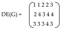
Since v31 0, v32 0 and the corresponding columns have an element (here ‘1’) in common, thus will be an edge of L(G) with degree d(1)+ d(2) - 2= 4. (original values of v3j are stored in a linear array).
To update the degrees of the corresponding edges of G [ i.e., the elements of the third row of DE(G) ] we replace v31 by v31-1 and v32 by v32 -1. We next compare the first column (provided v31-1 0) and the third column (since v33 0) of DE(G). The moment the updated value of v31 becomes zero, we move to the next column v3j , 2 j m , provided its updated value is non-zero.
The degree of in ELG = (deg of e1+deg of e2 in DE(G)) -2 = 3+3-2 = 4.
In this way we get the degree edge matrix [DEL(G)] of the line graph of the above graph as
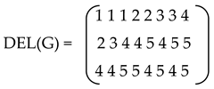
Figure 2.

The degree edge vector of the graph G is (3,3,3,4,3). We depict below how the degrees of the edges are changing when we implement Algorithm 1.
Degree edge vector Degree sum
(3 3 3 4 3 ) 16
(2 2 3 4 3 ) 14
(1 2 2 4 3 ) 12
(0 2 2 3 3 ) 10
(0 1 2 2 3 ) 8
(0 0 2 2 2 ) 6
(0 0 1 1 2 ) 4
(0 0 0 1 1 ) 2
(0 0 0 0 0 ) 0
The algorithm stops when the Degree sum becomes 0.
5. Line Graph of Directed Graph:
The concept of line graph of a graph can be extended to that of a digraph in an analogous way. But a difficulty arises in assigning a unique line digraph corresponding to a digraph, for there are three possible ways of defining the adjacency between any two arcs of a digraph. In fact, each of the following three types of adjacency (i) head-to-head, (ii) head-to-tail or tail-to-head and (iii) tail-to-tail corresponds to a line digraph and consequently they differ significantly. The convention is to accept “head-to-tail” adjacency for defining line graph of a digraph and we will stick to that. However, head-to-head and tail-to-tail adjacency relations are used in digraphs corresponding to food webs. Head-to head adjacency relation identifies species having common predators and thus the preys form Common enemy or Resource graphs; while tail-to tail adjacency relation identifies species having common preys and thus the predators form Competition or Consumer graphs [Mukherjee, 2010].
Definition 4. The degree of an arc ej =(vij,v2j), denoted by deg(ej), is defined by the out degree of the vertex v2j (i.e.,deg (ej)=d+ (v2j)).
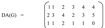
Definition 5. The degree arc matrix of a digraph, denoted by DA(G), is defined by
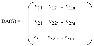
where the j th column ,1 j m, denote the j th arc emanating from the vertex v1j and converging to the vertex v2j, and v3j=deg(ej). The third row of DA(G) will be called the degree arc vector of a digraph G.
Thus to compare whether ej and ek are adjacent, we are to check whether v2j is identical with v1k. If ej and ek are adjacent, we shall update the degree of the arcs just by reducing the degree of ej by unity only (i.e,v3j is updated by v3j-1, but v3k remains same).
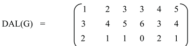
In DAL(G), the degree of the arc will be calculated from DAG as:
degree of the arc ek = out degree of v2k.
The degree arc matrix is
Here v31 0, so we compare between e1 and e2. Since v21 v12, we next compare and see that
v21 = v13, hence is an arc of the line digraph with degree2 ( since v33 = 2 ).
Since v31= 0 (updated value), we move to the second column and see that v32 0. We now compare e2 with e1 [although deg(e1) = 0 ].
Since v22 v11, we compare v22 with v13 and find v22 v13.
Next we see v22 = v14 . So is an arc of the line digraph with degree1.
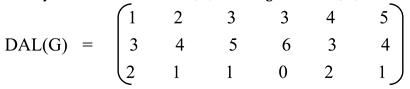
In this way we construct DAL(G) of the given DA(G) as
Algorithm for DAL(G) will differ from that of DEL(G) in the following points.
(i) If ej is adjacent to ek then only deg(ej) is updated.
(ii) To check whether ej is adjacent to ek, the columns of DAG are to be considered from the first column to the last column until (updated) v3j = 0. So k assumes the values 1,2,......j-1, j+1,....,m
Algorithm 2
Step 1 j=1
Step 2 If v3j = 0 then go to Step 10
Step 3 k= l
Step 4 If k = j then go to Step7.
Step 5 If the j th and the k th columns of DA(G) have one element in common
Then will be an arc in DAL(G) with degree deg(ek).
deg(ej) = deg(ej) – 1 /* Degree arc vector updated formulae*/
Step 6 If deg( ej) = 0 then go to Step10
Step 7 k = k+l
Step 8 If k > m then print" Error ": goto Step 14
Step 9 Go to Step 3
Step 10 j= j+l
Step 11 If j = m then print" Error ": go to Step 14
Step 12 Go to Step 2
Step 13 Print DAL(G).
Step 14. Stop.
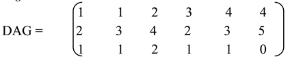
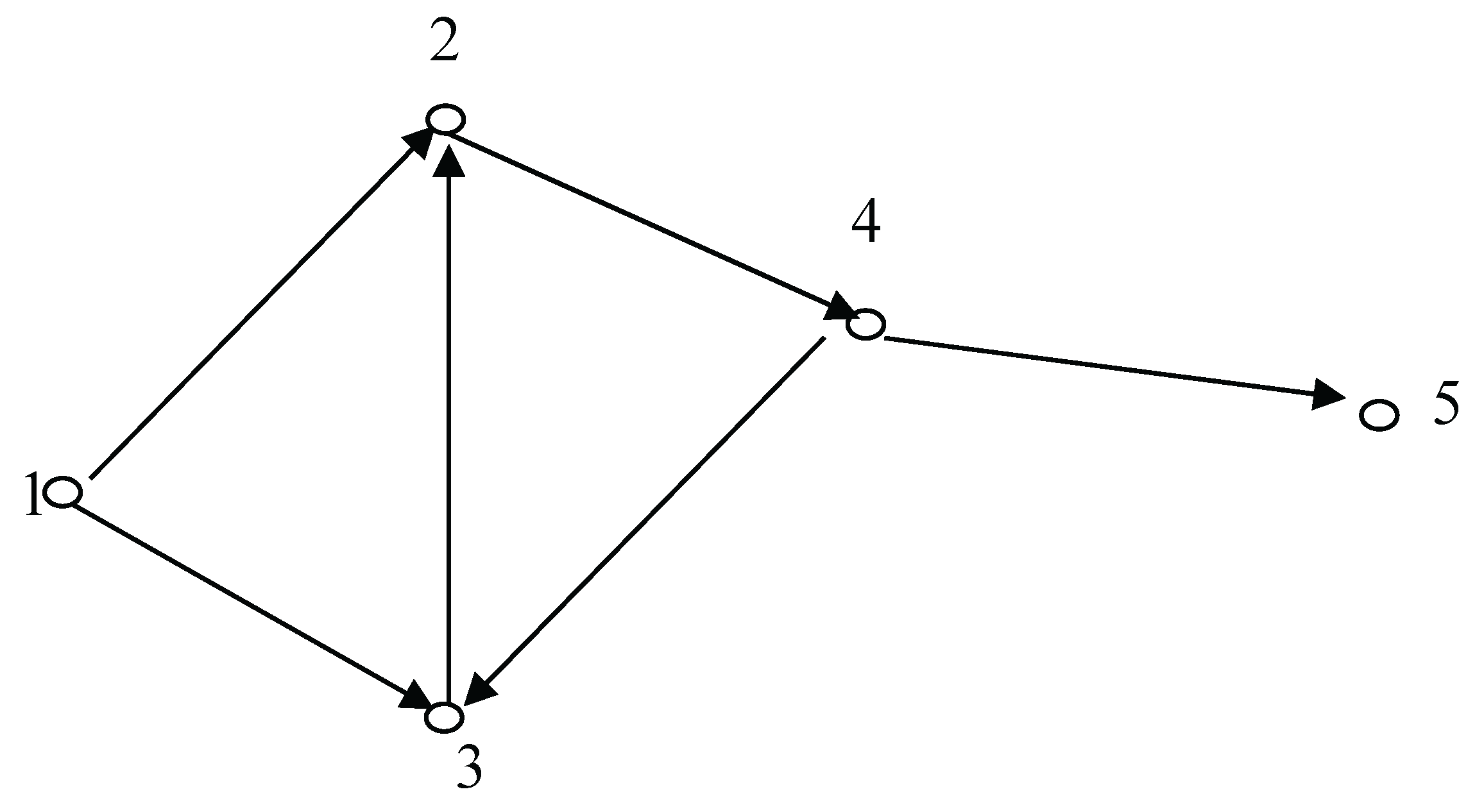
Illustration: 4 Let us consider the digraph as shown in Figure 3:
The degree arc matrix of the above digraph is
Here v31≠ 0, so we compare between e1 and e2. Since v21 ≠ v12, we next compare and see that v21 = v13, hence is an arc of the line digraph with degree 2 ( since v33=2).
We update the degree of the arc following Step 5. Since v31= 0 ( updated value), we move to the second column and see that v32≠ 0. We next compare e2 with e1 ( although deg(e1) = 0). Since v22 ≠ v11, we now compare v22 with v13 and see that v22 ≠ v13 and then find v22 = v14.
So will be an arc of the line digraph with degree 1.
In this way we construct DAL(G) from DA(G).
Illustration: 3: Let us consider the digraph
Figure 3.
So
The degree arc vector of the digraph is ( 2,1,1,0,2,1). We demonstrate below how the degrees of the arcs are changing when we implement Algorithm 2.
Degree arc vector Degree sum
(1 1 2 1 1 0 ) 6
(0 1 2 1 1 0 ) 5
(0 0 2 1 1 0 ) 4
(0 0 1 1 1 0 ) 3
(0 0 0 1 1 0 ) 2
(0 0 0 0 1 0 ) 1
(0 0 0 0 0 0 ) 0
The algorithm stops when the Degree sum becomes 0.
Conclusion
The time complexity of computing the line graph of an undirected graph with n vertices and m edges by Algorithm 1 is O(n4). This is due to the fact that the number of times the inner loop executed in the worst case is
= (m-1)+(m-2)+ ...+2+1=m(m-1)/2=O(m2) = O(n4), [ since m= O(n2).]
We have run programs in C corresponding to Algorithm 1 and Algorithm 2 where the inputs are the random graphs with varying threshold values. We have calculated the actual number of comparisons taking place in our method and then compared it with the method given in [3]. Apart from theoretical point of view, the outputs of the program show that our method is efficient from computational aspects as well. It has been found that the actual computing time is nearly 1% of the bound O(n4).
Appendix A
| OUTPUT OF THE PROGRAM | |||||||
| SL. NO. | N | THRESHOILD | DENSITY | OPERATIONS (EXISTING) | OPERATIONS (ACTUAL) | (%) TIME SAVING | |
| 1 | 6 | 0.67 | 0.2667 | 7776 | 39 | 99.4985 | |
| 2 | 7 | 0.56 | 0.2143 | 16807 | 56 | 99.6668 | |
| 3 | 8 | 0.34 | 0.2321 | 32768 | 80 | 99.7559 | |
| 4 | 12 | 0.78 | 0.4167 | 248832 | 1221 | 99.5093 | |
| 5 | 20 | 0.34 | 0.1684 | 3200000 | 1001 | 99.9687 | |
| 6 | 24 | 0.45 | 0.2391 | 7962624 | 3787 | 99.9524 | |
| 7 | 12 | 0.9 | 0.4773 | 248832 | 1591 | 99.3606 | |
| 8 | 15 | 0.45 | 0.2476 | 759375 | 903 | 99.8811 | |
| 9 | 18 | 0.88 | 0.4444 | 1889568 | 5157 | 99.7271 | |
| 10 | 8 | 0.99 | 0.4821 | 32768 | 414 | 98.7366 | |
| 11 | 20 | 0.9 | 0.4474 | 3200000 | 7347 | 99.7704 | |
| 12 | 15 | 0.88 | 0.4238 | 759375 | 2589 | 99.6591 | |
| 13 | 12 | 0.87 | 0.4394 | 248832 | 1350 | 99.4575 | |
| 14 | 18 | 0.34 | 0.1863 | 1889568 | 858 | 99.9546 | |
| 15 | 22 | 0.45 | 0.2186 | 5153632 | 2284 | 99.9557 | |
| 16 | 24 | 0.67 | 0.3514 | 7962624 | 7883 | 99.9010 | |
| 17 | 16 | 0.9 | 0.4542 | 1048576 | 3694 | 99.6477 | |
| 18 | 17 | 0.77 | 0.375 | 1419857 | 3098 | 99.7818 | |
| 19 | 8 | 0.99 | 0.4821 | 32768 | 422 | 98.7122 | |
| 20 | 6 | 0.44 | 0.2333 | 7776 | 25 | 99.6785 | |
| 21 | 14 | 0.88 | 0.4231 | 537824 | 2066 | 99.6159 | |
| 22 | 7 | 0.45 | 0.2143 | 16807 | 44 | 99.7382 | |
| 23 | 3 | 0.98 | 0.5 | 243 | 8 | 96.7078 | |
| 24 | 4 | 0.89 | 0.5 | 1024 | 32 | 96.8750 | |
| 25 | 5 | 0.33 | 0.1 | 3125 | 3 | 99.9040 | |
| 26 | 10 | 0.78 | 0.4333 | 100000 | 722 | 99.2780 | |
| 27 | 13 | 0.88 | 0.4423 | 371293 | 1795 | 99.5166 | |
| 28 | 19 | 0.33 | 0.1433 | 2476099 | 635 | 99.9744 | |
| 29 | 19 | 0.99 | 0.4971 | 2476099 | 7655 | 99.6908 | |
| 30 | 25 | 0.33 | 0.1367 | 9765625 | 1378 | 99.9859 | |
| 31 | 25 | 0.68 | 0.35 | 9765625 | 8950 | 99.9084 | |
| 32 | 21 | 0.5 | 0.231 | 4084101 | 2289 | 99.9440 | |
| 33 | 22 | 0.86 | 0.4264 | 5153632 | 8980 | 99.8258 | |
| 34 | 23 | 0.568 | 0.2747 | 6436343 | 4222 | 99.9344 | |
| 35 | 25 | 0.22 | 0.1117 | 9765625 | 888 | 99.9909 | |
| 36 | 6 | 0.67 | 0.1667 | 7776 | 14 | 99.8200 | |
| 37 | 6 | 0.99 | 0.5 | 7776 | 160 | 97.9424 | |
| 38 | 10 | 0.23 | 0.1 | 100000 | 24 | 99.9760 | |
| SL. NO. | N | THRESHOILD | DENSITY | OPERATIONS (EXISTING) | OPERATIONS (ACTUAL) | (%) TIME SAVING | |
| 39 | 10 | 0.61 | 0.3 | 100000 | 325 | 99.6750 | |
| 40 | 10 | 0.89 | 0.4444 | 100000 | 750 | 99.2500 | |
| 41 | 15 | 0.23 | 0.1 | 759375 | 153 | 99.9799 | |
| 42 | 15 | 0.61 | 0.3238 | 759375 | 1557 | 99.7950 | |
| 43 | 15 | 0.89 | 0.4667 | 759375 | 3137 | 99.5869 | |
| 44 | 25 | 0.19 | 0.0933 | 9765625 | 698 | 99.9929 | |
| 45 | 25 | 0.56 | 0.275 | 9765625 | 5496 | 99.9437 | |
| 46 | 25 | 0.92 . | 0.4417 | 9765625 | 4255 | 99.8540 | |
| 47 | 7 | 0.23 | 0.0714 | 16807 | 7 | 99.9584 | |
| 48 | 7 | 0.56 . | 0.3333 | 16807 | 120 | 99.2860 | |
| 49 | 7 | 0.95 | 0.5 | 16807 | 280 | 98.3340 | |
| 50 | 14 | 0.23 | 0.1319 | 537824 | 189 | 99.9649 | |
| 51 | 14 | 0.56 | 0.2582 | 537824 | 773 | 99.8563 | |
| 52 | 14 | 0.96 | 0.489 | 537824 | 2776 | 99.4838 | |
| 53 | 21 | 0.23 | 0.1119 | 4084101 | 549 | 99.9866 | |
| 54 | 21 | 0.67 | 0.3381 | 4084101 | 4817 | 99.8821 | |
| 55 | 21 | 0.89 | 0.4262 | 4084101 | 7656 | 99.8125 | |
| 56 | 8 | 0.23 | 0.125 | 32768 | 19 | 99.9420 | |
| 57 | 8 | 0.61 | 0.3393 | 32768 | 202 | 99.3835 | |
| 58 | 8 | 0.91 | 0.4821 | 32768 | 423 | 98.7091 | |
| 59 | 16 | 0.23 | 0.1625 | 1048576 | 495 | 99.9528 | |
| 60 | 16 | 0.67 | 0.3417 | 1048576 | 2070 | 99.8026 | |
| 61 | 16 | 0.89 | 0.4083 | 1048576 | 2927 | 99.7209 | |
| 62 | 26 | 0.36 | 0.1631 | 11881376 | 2109 | 99.9822 | |
| 63 | 26 | 0.96 | 0.4785 | 11881376 | 19002 | 99.8401 | |
| 64 | 9 | 0.23 | 0.1806 | 59049 | 87 | 99.8527 | |
| 65 | 9 | 0.61 | 0.2639 | 59049 | 174 | 99.7053 | |
| 66 | 9 | 0.92 | 0.4444 | 59049 | 520 | 99.1194 | |
| 67 | 11 | 0.23 | 0.1364 | 161051 | 87 | 99.9460 | |
| 68 | 11 | 0.65 | 0.3364 | 161051 | 587 | 99.6355 | |
| 69 | 11 | 0.92 | 0.4455 | 161051 | 1050 | 99.3480 | |
| 70 | 22 | 0.64 | 0.3203 | 5153632 | 5053 | 99.9020 | |
| 71 | 22 | 0.96 | 0.4784 | 5153632 | 11281 | 99.7811 | |
| 72 | 12 | 0.23 | 0.0909 | 248832 | 56 | 99.9775 | |
| 73 | 12 | 0.36 | 0.1591 | 248832 | 159 | 99.9361 | |
| 74 | 12 | 0.96 | 0.4924 | 248832 | 1714 | 99.3112 | |
| 75 | 24 | 0.23 | 0.1359 | 7962624 | 1122 | 99.9859 | |
| 76 | 24 | 0.61 | 0.3243 | 7962624 | 6743 | 99.9153 | |
| 77 | 24 | 0.98 | 0.4837 | 7962624 | 15163 | 99.8096 | |
| 78 | 13 | 0.23 | 0.0833 | 371293 | 53 | 99.9857 | |
| SL. NO. | N | THRESHOILD | DENSITY | OPERATIONS (EXISTING) | OPERATIONS (ACTUAL) | (%) TIME SAVING | |
| 79 | 13 | 0.64 | 0.3205 | 371293 | 975 | 99.7374 | |
| 81 | 26 | 0.23 | 0.1138 | 11881376 | 1029 | 99.9913 | |
| 82 | 26 | 0.64 | 0.32 | 11881376 | 8609 | 99.9275 | |
| 83 | 26 | 0.98 | 0.4862 | 11881376 | 19634 | 99.8347 | |
| 84 | 14 | 0.23 | 0.115454 | 537824 | 175 | 99.9675 | |
| 85 | 14 | 0.56 | 0.2308 | 537824 | 606 | 99.8873 | |
| 86 | 14 | 0.92 | 0.4725 | 537824 | 2596 | 99.5173 | |
| 87 | 28 | 0.23 | 1164 | 17210368 | 1342 | 99.9922 | |
| 88 | 28 | 0.63 | 0.3122 | 17210368 | 10216 | 99.9406 | |
| 89 | 28 | 0.91 | 0.4563 | 17210368 | 21896 | 99.8728 | |
| 90 | 16 | 0.23 | 0.15 | 1048576 | 375 | 99.9642 | |
| 91 | 16 | 0.65 | 0.3 | 1048576 | 1638 | 99.8438 | |
| 92 | 16 | 0.96 | 0.4792 | 1048576 | 4110 | 99.6080 | |
| 93 | 28 | 0.36 | 1799 | 17210368 | 3454 | 99.9799 | |
| 94 | 28 | 0.96 | 0.4894 | 17210368 | 25118 | 99.8541 | |
| 95 | 17 | 0.23 | 0.1287 | 1419857 | 393 | 99.9723 | |
| 96 | 17 | 0.61 | 0.3309 | 1419857 | 2326 | 99.8362 | |
| 97 | 17 | 0.92 | 0.4522 | 1419857 | 4467 | 99.6854 | |
| 98 | 29 | 0.23 | 0.1182 | 20511149 | 1661 | 99.9919 | |
| 99 | 29 | 0.63 | 0.3005 | 20511149 | 10349 | 99.9495 | |
| 100 | 29 | 0.96 | 0.4766 | 20511149 | 26541 | 99.8706 | |
| 101 | 18 | 0.23 | 0.1307 | 1889568 | 477 | 99.9748 | |
| 102 | 18 | 0.61 | 0.317 | 1889568 | 2654 | 99.8595 | |
| 103 | 18 | 0.92 | 0.4739 | 1889568 | 5852 | 99.6903 | |
| 104 | 19 | 0.23 | 0.0848 | 2476099 | 214 | 99.9914 | |
| 105 | 19 | 0.62 | 0.3216 | 2476099 | 3284 | 99.8674 | |
| 106 | 19 | 0.95 | 0.4561 | 2476099 | 6442 | 99.7398 | |
| 107 | 25 | 0.22 | 0.1117 | 9765625 | 888 | 99.9909 | |
| 108 | 6 | 0.67 | 0.1667 | 7776 | 14 | 99.8200 | |
| 109 | 6 | 0.99 | 0.5 | 7776 | 160 | 97.9424 | |
| 110 | 6 | 0.19 | 0 | 7776 | 0 | 100.0000 | |
| 111 | 10 | 0.23 | 0.1 | 100000 | 24 | 99.9760 | |
| 112 | 10 | 0.61 | 0.3 | 100000 | 325 | 99.6750 | |
| 113 | 10 | 0.89 | 0.4444 | 100000 | 750 | 99.2500 | |
| 114 | 15 | 0.23 | 0.1 | 759375 | 153 | 99.9799 | |
| 115 | 15 | 0.61 | 0.3238 | 759375 | 1557 | 99.7950 | |
| 116 | 15 | 0.89 | 0.4667 | 759375 | 3137 | 99.5869 | |
| 117 | 25 | 0.19 | 0.0933 | 9765625 | 698 | 99.9929 | |
| 118 | 25 | 0.56 | 0.275 | 9765625 | 5496 | 99.9437 | |
| 119 | 25 | 0.92 . | 0.4417 | 9765625 | 4255 | 99.8540 | |
| 120 | 7 | 0.23 | 0.0714 | 16807 | 7 | 99.9584 | |
| 123 | 14 | 0.23 | 0.1319 | 537824 | 189 | 99.9649 | |
| 124 | 14 | 0.56 | 0.2582 | 537824 | 773 | 99.8563 | |
| SL. NO. | N | THRESHOILD | DENSITY | OPERATIONS (EXISTING) | OPERATIONS (ACTUAL) | (%) TIME SAVING | |
| 125 | 14 | 0.96 | 0.489 | 537824 | 2776 | 99.4838 | |
| 126 | 21 | 0.23 | 0.1119 | 4084101 | 549 | 99.9866 | |
| 127 | 21 | 0.67 | 0.3381 | 4084101 | 4817 | 99.8821 | |
| 128 | 21 | 0.89 | 0.4262 | 4084101 | 7656 | 99.8125 | |
| 129 | 8 | 0.23 | 0.125 | 32768 | 19 | 99.9420 | |
| 130 | 8 | 0.61 | 0.3393 | 32768 | 202 | 99.3835 | |
| 131 | 8 | 0.91 | 0.4821 | 32768 | 423 | 98.7091 | |
| 132 | 16 | 0.23 | 0.1625 | 1048576 | 495 | 99.9528 | |
| 133 | 16 | 0.67 | 0.3417 | 1048576 | 2070 | 99.8026 | |
| 134 | 16 | 0.89 | 0.4083 | 1048576 | 2927 | 99.7209 | |
| 135 | 26 | 0.36 | 0.1631 | 11881376 | 2109 | 99.9822 | |
| 136 | 26 | 0.96 | 0.4785 | 11881376 | 19002 | 99.8401 | |
| 137 | 9 | 0.23 | 0.1806 | 59049 | 87 | 99.8527 | |
| 138 | 9 | 0.61 | 0.2639 | 59049 | 174 | 99.7053 | |
| 139 | 9 | 0.92 | 0.4444 | 59049 | 520 | 99.1194 | |
| 140 | 11 | 0.23 | 0.1364 | 161051 | 87 | 99.9460 | |
| 141 | 11 | 0.65 | 0.3364 | 161051 | 587 | 99.6355 | |
| 142 | 11 | 0.92 | 0.4455 | 161051 | 1050 | 99.3480 | |
| 143 | 22 | 0.64 | 0.3203 | 5153632 | 5053 | 99.9020 | |
| 144 | 22 | 0.96 | 0.4784 | 5153632 | 11281 | 99.7811 | |
| 145 | 12 | 0.23 | 0.0909 | 248832 | 56 | 99.9775 | |
| 146 | 12 | 0.36 | 0.1591 | 248832 | 159 | 99.9361 | |
| 147 | 12 | 0.96 | 0.4924 | 248832 | 1714 | 99.3112 | |
| 148 | 24 | 0.23 | 0.1359 | 7962624 | 1122 | 99.9859 | |
| 149 | 24 | 0.61 | 0.3243 | 7962624 | 6743 | 99.9153 | |
| 150 | 24 | 0.98 | 0.4837 | 7962624 | 15163 | 99.8096 | |
| 151 | 13 | 0.23 | 0.0833 | 371293 | 53 | 99.9857 | |
| 152 | 13 | 0.64 | 0.3205 | 371293 | 975 | 99.7374 | |
| 153 | 13 | 0.89 | 0.4615 | 371293 | 1918 | 99.4834 | |
| 154 | 26 | 0.23 | 0.1138 | 11881376 | 1029 | 99.9913 | |
| 155 | 26 | 0.64 | 0.32 | 11881376 | 8609 | 99.9275 | |
| 156 | 26 | 0.98 | 0.4862 | 11881376 | 19634 | 99.8347 | |
| 157 | 14 | 0.23 | 0.115454 | 537824 | 175 | 99.9675 | |
| 158 | 14 | 0.56 | 0.2308 | 537824 | 606 | 99.8873 | |
| SL. NO. | N | THRESHOILD | DENSITY | OPERATIONS (EXISTING) | OPERATIONS (ACTUAL) | (%) TIME SAVING | |
| 159 | 14 | 0.92 | 0.4725 | 537824 | 2596 | 99.5173 | |
| 160 | 28 | 0.23 | 1164 | 17210368 | 1342 | 99.9922 | |
| 161 | 28 | 0.63 | 0.3122 | 17210368 | 10216 | 99.9406 | |
| 165 | 16 | 0.96 | 0.4792 | 1048576 | 4110 | 99.6080 | |
| 166 | 28 | 0.36 | 1799 | 17210368 | 3454 | 99.9799 | |
| 167 | 28 | 0.96 | 0.4894 | 17210368 | 25118 | 99.8541 | |
| 168 | 17 | 0.23 | 0.1287 | 1419857 | 393 | 99.9723 | |
| 169 | 17 | 0.61 | 0.3309 | 1419857 | 2326 | 99.8362 | |
| 170 | 17 | 0.92 | 0.4522 | 1419857 | 4467 | 99.6854 | |
| 171 | 29 | 0.23 | 0.1182 | 20511149 | 1661 | 99.9919 | |
| 172 | 29 | 0.63 | 0.3005 | 20511149 | 10349 | 99.9495 | |
| 173 | 29 | 0.96 | 0.4766 | 20511149 | 26541 | 99.8706 | |
| 174 | 18 | 0.23 | 0.1307 | 1889568 | 477 | 99.9748 | |
| 175 | 18 | 0.61 | 0.317 | 1889568 | 2654 | 99.8595 | |
| 176 | 18 | 0.92 | 0.4739 | 1889568 | 5852 | 99.6903 | |
| 177 | 19 | 0.23 | 0.0848 | 2476099 | 214 | 99.9914 | |
| 178 | 19 | 0.62 | 0.3216 | 2476099 | 3284 | 99.8674 | |
| 179 | 19 | 0.95 | 0.4561 | 2476099 | 6442 | 99.7398 | |
| 180 | 3 | 0.66 | 0.3333 | 243 | 1 | 99.5885 | |
| 181 | 8 | 0.1234 | 0.0714 | 32768 | 8 | 99.9756 | |
| 182 | 10 | 0.2513 | 1333 | 100000 | 56 | 99.9440 | |
| 183 | 9 | 0.236 | 0.0972 | 59049 | 27 | 99.9543 | |
| 184 | 16 | 0.369 | 2083 | 1048576 | 712 | 99.9321 | |
| 185 | 18 | 0.1234 | 0.0621 | 1889568 | 74 | 99.9961 | |
References
- Beineke.L.W (1970) - Characterizations of derived graphs -J.Comb.Theory,vol -9, pp. 129 -135.
- Chartrand.G and Oellermann (1993) - Applied and algorithmic graph theory- Mc Graw Hill Inc.
- Harary.F (1994) - Graph theory.Addison -Wesley publishing co.
- Hemminger.R.L and Beineke. L.W.( 1978) - Line graphs and digraphs- Selected topics in graph theory ( L.W.Beineke and R.J.Wilson,eds.),Academic press, pp.271 -305.
- Krawczyk. M.J, Muchnik. L, Mańka-Krasoń. A and. Kułakowski. K. ( 2011) - Line graphs as social networks-Physica A: Statistical Mechanics and its Applications, Volume 390, Issue 13, pp. 2611-2618.
- Kumar. V, Sardana. S and Madan. A.K.-( 2010)- Numerical characterization of DNA sequences: connectivity type indices derived from DNA line graphs- J. of Mathematical Chemistry, Volume 48, Number 3, pp. 521-529.
- Fish.W, Kumwenda.K and Mwambene. E. ( 2011) - Codes and designs from triangular graphs and their line graphs- Central European J. of Mathematics, Volume 9, Number 6, pp.1411-1423.
- Mukherjee.P ( 2010) - Studies on Food Webs Using Matrices Associated With Graphs- Int. J. of Appl. Env.Sc., ISSN 0973-6077 Volume 5, Number 4, pp. 603–608, RIP.
- Sabidussi.G.( 1961) - Graph derivatives - Math. Z, vol - 76, pp. 385 - 401.
- Tatsuo. O, Hajimu. M; Ernest S. K, Toshinobu,K and Toshio.F. ( 1979)- One-.
- dimensional logic gate assignment and interval graphs- IEEE Transactions on Circuits.
- and Systems 26 (9), pp. 675–684.
- Weiss. M.k. ( 2001)- Data Structures and Algorithm Analysis in C- Addison-Wesley.
- West. D.B. ( 2000) - Introduction to Graph Theory- PHI, New Delhi, 2000.
Figure 1.
Disclaimer/Publisher’s Note: The statements, opinions and data contained in all publications are solely those of the individual author(s) and contributor(s) and not of MDPI and/or the editor(s). MDPI and/or the editor(s) disclaim responsibility for any injury to people or property resulting from any ideas, methods, instructions or products referred to in the content. |
© 2025 by the authors. Licensee MDPI, Basel, Switzerland. This article is an open access article distributed under the terms and conditions of the Creative Commons Attribution (CC BY) license (http://creativecommons.org/licenses/by/4.0/).
Copyright: This open access article is published under a Creative Commons CC BY 4.0 license, which permit the free download, distribution, and reuse, provided that the author and preprint are cited in any reuse.


