Submitted:
06 June 2025
Posted:
09 June 2025
You are already at the latest version
Abstract
Background: Achieving malaria elimination requires identifying hotspots and key risk factors to guide targeted interventions. In this context, spatial models are crucial to support decision making. Yet, in elimination settings, national-level models suffer from some limitations. They often rely on prevalence survey data, which may be less reliable in low-transmission settings due to excess zeroes and under-representation of high-risk age groups. In addition, they often assume stationary risk factors, while pre-elimination strategies may lead to the emergence of (temporarily) distinct endemic profiles within countries. To address these biases, we model malaria incidence in Senegal, targeting malaria elimination for 2030, using routine malaria data and stratifying models by transmission level. Methods: Malaria incidence rates by health facility were calculated using reported cases and estimated catchment population, allowing for overlap between health facility catchment areas. Malaria incidence was then modelled using fine-resolution environmental and socio-economic covariates within a Bayesian hierarchical framework implemented using the INLA-SPDE approach. Models were stratified by season and endemicity level and compared with a national benchmark model to assess the heterogeneity of malaria risk factors. Finally, dasymetric disaggregation was applied to generate high-resolution (1 km) maps of malaria incidence. Results: The modelled incidence of malaria decreased by three cases per 1,000 people between 2017 (47 per 1,000 people) and 2019 (44 per 1,000 people), before increasing by 15 cases per 1,000 people in 2021 (59 per 1,000 people). At the sub-national level, malaria incidence followed an increasing gradient from the urbanised north-west to the south-eastern regions. Despite comparatively low seasonal variation in malaria risk factors, the importance of specific risk factors varied across areas with different levels of endemicity. Some factors (e.g. precipitation, ethnicity and urban agriculture) were particularly associated with either low, moderate, or high transmission settings. Fine-scale maps of the posterior estimates show higher malaria incidence for areas closer to a health facility than those further away, thus highlighting potential underdiagnosis of malaria in remote areas. Conclusion: Our findings underscore the importance of taking both endemicity and risk factors into account while evaluating malaria incidence. This approach allows the identification of risk factors specific to each endemicity level, essential for the design and implementation of more effective targeted interventions. In the near future, as prevalence data become less reliable and the quality of health system data continues to improve, fine-scale incidence models and maps will become critical tools to support decision-making.
Keywords:
malaria
; Senegal
; Bayesian geostatistical modelling
; routine health facility data
; malaria incidence
; catchment areas
Introduction
In 2023, malaria was still the deadliest vector-borne disease, responsible for 597,000 deaths worldwide, 95% of which occurred in sub-Saharan Africa (SSA) and most of which were due to Plasmodium falciparum [1]. Insecticide-treated nets (ITNs) and artemisinin-based combination therapies (ACTs), combined with huge control efforts [2,3], have reduced the burden of malaria from 864,000 to 586,000 deaths between 2000 and 2015 [1]. Over this period, malaria incidence was reduced by up to 50-75% in several high-burden countries [3,4]. Yet, malaria deaths have stalled since 2015 and have even increased since the COVID-19 pandemic due to disruptions in health services and intervention planning that have had latent effects until very recently [1]. An increasing number of countries are now in the process of malaria elimination, with 35 countries committing to do so by 2030 under the Global Technical Strategy for Malaria 2016-2030 [5] and in line with Sustainable Development Goal Target 3.3, which includes reducing malaria incidence by at least 90% by 2030 [6].
Achieving malaria elimination requires identifying the factors that perpetuate the disease hotspots, as they can help identify leverage points for more effective intervention planning. Previous studies have modelled malaria prevalence or incidence at the national level and identified contributing risk factors in Ghana [7,8], Rwanda [9], Nigeria [10,11], Mozambique [12,13], Senegal [14], Uganda [15,16], Zambia [17,18] and Cameroon [19]. Yet national-level models assume spatial stationarity of malaria-determinants relationships and correlation structures [20], whereas a few studies have shown that relationships with malaria and vector-borne diseases in general may vary according to several factors, such as mosquito vector species [21], season [22], or the scale considered (household, regional or national) [21,23,24], also known as the Modifiable Areal Unit Problem (MAUP) [25]. Relationships may also vary between different geographical contexts, as environmental and human factors may interact. This is illustrated by the ‘paddies paradox’, where rice paddy irrigated areas may be associated with lower malaria incidence due to improved socioeconomic conditions and changes in the main mosquito species [26]. Transmission drivers may differ between lowland and highland areas [20,21] or between urban and rural settings [27], as well as between cities [28,29].
Pertaining to the geographical context, the level of endemicity can significantly influence both the strength of and relationships with malaria [30]. Endemicity directly affects immunity in children and adults, which means that adults in areas with different levels of endemicity may be more or less at risk of malaria [31], and the risk factors may not be the same (e.g. adult migration may be more of a risk factor in low-endemic areas). Accounting for endemicity levels when analysing malaria risk factors is therefore essential, especially considering that malaria control and elimination interventions and their effects vary according to the level of transmission (e.g. seasonal chemoprevention in highly endemic areas and case investigation in low endemic areas) [3]. For example, [32] showed that the interaction between seasonality and level of endemicity influences malaria repeat episodes and should therefore influence the choice of ACT duration. Stakeholder needs may also depend on the spatial scale [33]. In addition, as (pre-)elimination interventions are progressively implemented within countries, and depending on their success, differences in endemicity between regions may become more pronounced.
Fine-scale malaria models are often based on household surveys that test malaria in nationally representative samples, such as the Demographic and Health Surveys (DHS) or the Malaria Indicator Surveys (MIS). Such surveys provide estimates of malaria prevalence among the individuals tested (usually children under 5 years of age). Although these surveys offer the possibility of regular updates as they are conducted on a regular basis [34], they suffer from two main biases: first, in low transmission settings, samples contain excess zeros due to the rare occurrence of the disease [35,36], and second, adolescents and adults are not included in the testing, whereas malaria elimination would require knowledge of the malaria burden in all age groups [37]. Alternatively, routine data collected monthly by health facilities can be used to estimate malaria incidence, providing continuous estimates over time and over large spatial scales [38]. Although these data also suffer from known biases such as under-reporting, low testing rate and missing the population that does not seek health care [35,38], they are an important source of epidemiological data on malaria, particularly in areas where prevalence may be less representative or reliable [36]. In recent years, studies have begun to investigate the use of such surveillance data for spatio-temporal modelling and fine-scale prediction of malaria incidence [39,40,41,42]. Such predictive maps can help to identify malaria hotspots, guide intervention strategies and optimise health resource allocation. In this study, we propose to use dasymetric disaggregation, a method commonly used to disaggregate population census estimates [43,44], to produce fine-scale maps of malaria incidence. This approach relies on the redistribution of reported malaria cases from health facilities to a finer spatial resolution, thereby improving the granularity of risk estimates.
With the goal of malaria elimination by 2030, Senegal has reduced malaria incidence and mortality in recent decades thanks to improved malaria control [4,45]. Despite significant efforts, malaria cases have stagnated and even increased from 2019 [45], leading to an estimated 2128 deaths and 831 514 cases in 2022, accounting for 0.35% of the global mortality burden [1]. However, these national estimates mask further heterogeneity at the sub-national level, as Senegal has a highly heterogeneous malaria endemic profile, lying in the transition zone between the low, intermediate and high endemic regions of West Africa. Three major endemicity groups can be distinguished (see Figure 1) [45]: 1) the rural south-eastern regions (Kolda, Kédougou, Tambacounda, collectively known as the KKT area) with high malaria transmission, representing only 12% of the total population but 65% of total malaria cases, 2) the western highly urbanised regions (Dakar, Diourbel, Kaolack) with intermediate transmission accounting for 30% of the national case burden and 3) the northern regions with low to very low malaria transmission and some areas classified as pre-elimination [45]. The strong heterogeneity in endemicity levels across the country is likely to bias national malaria models. For example, [46] showed that national population models in Senegal under-represented rural areas due to significant differences in population predictors between rural and urban areas and the high urban-rural divide in the country. Malaria cases in Senegal are reported through the District Health Surveillance System (DHIS2) platform, which maintained high reporting rates until 2021 (98%), but saw a significant drop to 27% in 2023 due to health worker strikes [47].
The aim of this research is to model malaria incidence in Senegal from 2017 to 2021, using routine data from the DHIS2 platform and a set of high-resolution environmental and socio-economic variables. A key challenge in working with routine health facility data is the need to define catchment areas around health facilities to estimate population denominators. In this study, we account for this uncertainty by incorporating the probability of attending a health facility based on relative walking time, rather than assuming fixed, non-overlapping catchment boundaries. Spatio-temporal models of malaria incidence are then built within a Bayesian hierarchical framework implemented using the INLA-SPDE approach. Models are stratified by season and endemicity level and compared with a benchmark model at the national level to assess potential heterogeneity of malaria risk factors according to the transmission level, which may vary in time (i.e. per season) and space (i.e. per endemicity level). Lastly, dasymetric disaggregation is applied to generate high-resolution (1 km) maps of malaria incidence that can help support targeted intervention planning. The method of [43] is adapted by considering the probability of attending a health facility and the pixel population in the disaggregation weights.
Material and Methods
Routine Malaria Data
Routine malaria data were extracted from the DHIS2 platform for the period 2017-2021 by the Laboratoire Dynamiques territoriales et Santé of Cheikh Anta Diop University of Dakar (Senegal). We used this period because annual reporting rates consistently exceeded 95% (see S1 Table) [45]. From 2022, health worker strikes led to a significant drop in reporting rates (e.g. to 27% in 2023), making routine data unreliable for analysis [47]. Data are available as malaria cases in all age groups, confirmed by RDT, per month and per health facility. In this study, only public facilities (health centres, health posts, hospitals and garrison medical centres) were included, as done in [39,48], as most Senegalese (75%) who seek treatment for fever do so in the public sector (22% in the private sector and 3% in traditional medicine and others) (estimates based on DHS 2017 [49]). In addition, not all private facilities are registered on the DHIS2 platform, unlike public facilities, which are legally required to report data. Public health facilities with missing case data for the entire time series (2017 to 2021) (8% of public health facilities) were excluded from the analysis due to ambiguity in their interpretation [50]; missing values could indicate that no cases were ever observed, cases were not reported at the facility, the facility was not equipped for malaria testing, or the facility is closed but not removed from the DHIS2 platform. Facilities were geolocated using the database of [51], which consolidated geolocated health facility data for Senegal by combining several sources, such as a spatial database of public health sector for SSA [52] and Service Provision Assessment surveys from the DHS Program. Any facility missing from this database was manually verified using OpenStreetMap and Google Maps. In total, 90% of public health facilities with reported cases (n = 1,472) were successfully geolocated (see S1 Figure and S1 Table for details by region), leaving only 10 % of malaria cases not geolocated (n = 232,338). For each year, we calculated per health facility 1) the total number of cases, 2) the total number of cases during the dry season (from November to May), and 3) the total number of cases during the wet season (from June to October).
Geospatial Covariate Data
DHS Variables and Processing
The DHS provides estimates of key variables that influence malaria risk and are related to individuals' socioeconomic status and access to malaria prevention. The DHS uses a two-stage stratified sampling frame based on region and rural/urban areas within regions. Primary sampling units (PSUs), defined based on census enumeration areas, are selected within each stratum with probability proportional to population size, and 25-30 households within each PSU are further selected for questionnaire interviews [34,53].
In this study, we used data from the most recent household surveys conducted in Senegal: the 2017, 2018, 2019 continuous DHS, the 2020-2021 Malaria Indicator Survey (MIS) (conducted mostly in 2020 and early 2021), and the 2023 continuous DHS. We selected several indicators that may influence susceptibility to malaria and resilience (e.g., capacity to anticipate the disease): proportion of Fula people, access to basic sanitation, stunting in children, insecticide-treated net (ITN) ownership and literacy rate in women. These indicators were aggregated at the cluster level following the instructions of the survey reports and the DHS program [34]. They are listed in Table 1 and described in more detail in supplementary material.
To generate interpolated surfaces for these indicators, we used spatio-temporal Bayesian models without covariates to avoid circularity issues when later modelling malaria incidence, as recommended by [60]. Consider as the number of individuals with a given condition or characteristic of interest (e.g. stunted children, households with at least one ITN, etc.) out of , the number of individuals surveyed in survey cluster for year , corresponding to the years 2017 to 2021). Given the true proportion , follows a binomial distribution:
where is the intercept. is a spatially structured random effect modelled as a zero-mean Gaussian Process (GP) such that [61]. Spatial dependence between two observations of the GP is modelled using the Matérn covariance function (defined in S1 Text) with range and marginal variance [61]. is the temporally structured random effect, modelled as an autoregressive process of order 1 (AR(1)) with and [61,62]. is the autoregressive coefficient and is a zero-mean Gaussian noise term with variance . Weekly informative priors were assigned to parameters and hyperparameters: , , , and . is the maximum distance (in degrees) measured across the study area.
The 2020–2021 MIS data were primarily treated as representing 2020, and interpolated surfaces were projected for 2021 using the model. Model performance was evaluated using two cross-validation techniques: 1) 5-repeated 5-fold random cross-validation and 2) temporal block cross-validation (i.e. leaving out one year of observations at a time to assess the model's ability to predict over time) following [40]. The following metrics were computed on the posterior mean estimates of the test sets: the mean absolute error (MAE), the root mean square error (RMSE), the coefficient of determination (R²) and the squared correlation between predicted and observed values (r²).
Remotely Sensed Variables
A set of gridded environmental and socioeconomic covariates influencing malaria incidence was extracted from open-source repositories. Except for time-invariant covariates (e.g. climatic averages, elevation), data were obtained for the years 2017 to 2021. Covariates were resampled to a common 1×1 km grid resolution to ensure spatial alignment across datasets and in subsequent analyses. All covariates are listed in Table 1 and described in more detail in the supplementary material.
Catchment Population
Computation of Travel Time
Estimates of travel time to public health facilities are needed at several stages in this study workflow, especially to estimate the population seeking care and the catchment areas of health facilities, which are detailed below. In this study, people were assumed to walk to the health facility of their choice. In Senegal, 81% of people travel to the nearest health facility by non-motorised means (70% walk) and less than 10% of households own a car (estimates based on DHS 2023 [63]). Similarly, a survey to understand health access behaviour for malaria in SSA found that most participants chose to walk to their health facility, with walking times of up to 50 minutes [64].
Travel time was calculated by adapting the methodology used by Alegana et al. 2012 [65]. Walking time was calculated considering slope, land cover, roads and rivers. First, the slope was calculated based on a digital elevation model [59]. Travel speed (km/h) is then calculated as a function of slope using Tobler’s hiking function [66], assuming an individual walks at 5 km/h on a flat surface:
As travel speed also depends on land cover, with some categories being easier to cross (e.g. built-up areas compared to trees, rivers impassable, etc.), these travel speeds were adjusted according to walking speeds from [67] (see Table 2). Lastly, using the gdistance package in R statistical programming software, travel speeds were converted into conductance values (i.e. the inverse of travel time), which were then used to calculate gridded travel time estimates to health facilities (from 2017 to 2021) using a least cost algorithm (accost function).
Treatment-Seeking Population
Gridded population counts have been extracted from the WorldPop project (www.worldpop.com) for the years 2017 to 2020. These grids, available at a spatial resolution of 100 m, were derived by disaggregating census data using Random Forest-based dasymetric redistribution with various geospatial covariates (e.g. land use and land cover, night lights, etc.) [68,69]. As years beyond 2020 were not available, population counts were projected for the year 2021 by fitting a simple exponential model assuming exponential population growth. Population counts were resampled to the same 1x1 km resolution grid used for resampling geospatial covariates.
In Senegal, only 39% of people seek care at public health facilities when their child has a fever, while 48% do not seek care at all (estimates based on DHS 2017 [49]). As a result, using the total population as the denominator may bias the estimates of malaria incidence. To account for this, we used data on attendance at public health facilities among children with fever from the 2017, 2018, 2019 and 2023 DHS and the 2020-2021 MIS. We modelled attendance at public health facilities , where indicates attendance and indicates non-attendance, as a function of travel time using a Bayesian logistic regression model. The random variable follows a Bernoulli distribution with probability of attending a public health facility for a child with fever in year , corresponding to the years 2017 to 2021). The model is expressed as follows:
where is the intercept, is the minimum walking time to a public health facility from location of child in year and is its regression coefficient, with as prior. The rest of the parameters are defined as for (1).
Model performance was assessed through 5-repeated 5-fold cross-validation and temporal block cross-validation by calculating the accuracy (proportion of correct predictions to all predictions), precision (proportion of true positives to all positive predictions), recall (proportion of true positives to all actual positives) and the Area Under Curve (AUC). Using the fitted model, we generated interpolated surfaces of the probability of attending a public health facility for the years 2017 to 2021. The population seeking health care was calculated by multiplying the population counts by the gridded probability, following previous work [42,65].
As not all facilities with reported cases could be geolocated, the population estimates were also adjusted to account for these missing cases, especially as the proportion of geolocated cases varied between regions, with geolocation of health facilities more difficult to obtain in rural and remote areas. Therefore, a regional case geolocation rate (i.e. the proportion of cases that were geolocated) was calculated and applied uniformly to the gridded estimates of the population seeking health care. Finally, we made no further adjustments regarding health facility reporting rates, as reporting completeness remained above 95% throughout the study period and the remaining 5% was accounted for in the modelling stage. This decision helped to prevent the introduction of additional sources of bias.
Overlapping Catchment Areas
In this study, we define the catchment population of a health facility as the group of people who attend that facility for treatment of fever symptoms. We refer to the ‘total potential catchment population’ as the group of people who would attend that facility for fever treatment if 100% of the population sought health care for fever. Since health facility catchments are not directly observed, they must be estimated to determine the catchment population for each facility. A common approach is to assign populations to the nearest facility based on travel time or distance (e.g. through Voronoi polygons). This method is straightforward, easy to implement and allows clear visualisation [70,71]. However, it relies on strong assumptions that do not fully reflect reality, as factors other than travel time influence the choice of health facility (e.g. type of facility, quality of service offered, patient habits, etc.) [70,71]. This approach may also result in facilities not being assigned a catchment population because they are not the closest facility to any population, despite having recorded malaria cases. In addition, in urban areas where the density of health facilities is high, the catchment population of centrally located facilities may be systematically underestimated (especially for hospitals, which tend to attract more patients), as commuters are exclusively assigned to suburban health facilities [50]. For these reasons, and after experimentation, we decided to allow health facilities to have overlapping catchment areas, assuming that individuals may choose between multiple health facilities, although this choice still depends on the relative travel time to these facilities.
We used the methodology described in [39]. First, we divided the study area into pixels of 1x1 km and summed the cases of health facilities located in the same pixel [48,50]. The probability of a treatment-seeking individual in populated pixel attending health facility (HF) depends on the travel time to that health facility, but also on the travel times to other facilities:
where is the probability of an individual in pixel attending health facility ; is the walking time from pixel to health facility ; and is the number of health facilities. By design, the probability of walking to each facility sums to 1 for each pixel. A limitation of this approach is that all pixels are calculated with a non-zero probability of going to any facility, even if the facility is realistically out of reach (e.g. 400 minutes away). We slightly improved this method by considering that a person in pixel is likely to go to any facility that is within 30 minutes of their home with a probability computed with (4), or to the closest facility if the walking time is greater than 30 minutes (i.e. with a probability equal to 1). This 30-minute threshold was chosen because 75% of people have the nearest health facility less than 30 minutes from their home (estimates based on DHS 2023 [63]). The catchment population of health facility was then calculated as follows:
where is the population in pixel attending facility , and is the number of populated pixels with a non-zero probability of attending facility j. Separate catchment areas were generated for each year from 2017 to 2021 using annually updated travel time data, as previously calculated. For a given year , we considered all facilities that reported cases in year , as well as those that reported cases in any previous year but may have missing cases in year . S2 Figure illustrates an example of catchment areas delineated using this method. In panel (a), overlapping catchment areas are observed in regions with a high density of health facilities, while panel (b) shows an example from a low-density setting where catchment areas do not overlap.
Covariate Extraction
For land use and land cover (LULC) covariates, we extracted the proportion of different LULC classes in the delimited catchments. For all other covariates, we extracted the mean values in the catchment area after masking out water pixels. Continuous covariates were standardised (z-score transformation) to ensure comparability across different measurement scales.
Incidence Model
Model Structure
Malaria incidence rates (MIR) were modelled using a Bayesian hierarchical framework that allows quantifying the effects of socioeconomic and environmental covariates on MIR, while simultaneously accounting for spatial and temporal random variation. After estimating catchment populations, the malaria incidence rate (MIR) at health facility for year , i.e. from 2017 to 2021) was calculated as follows:
where is the number of cases reported at facility in year and is the catchment population of facility in year . MIR in Senegal present a highly right-skewed distribution, with many values close to zero in low and very low transmission settings and a few MIR values greater than 1 in the high transmission areas due to repeated malaria episodes [32] and significant cross-border migration [72]. We therefore used the log-transformed MIR as the dependent variable, which was found to follow a normal distribution (see S3 Figure), so that:
where is the variance of the measurement error, is the intercept, is the vector of covariates at the location of facility and year and is a vector of the corresponding coefficients. is defined as a zero-mean Gaussian process representing uncorrelated random variations in time and space. is a spatio-temporal random effect changing in time with first order autoregressive dynamics and spatially correlated random variations [73,74]. It is formulated as follows [73,74]:
where with autoregressive coefficient and is the marginal variance of the Gaussian field . is assumed to be temporally independent and has the following spatio-temporal covariance function [73,74]:
where is the Matérn covariance function (defined in S1 Text). For common parameters as in (1), we used similar priors except for . was defined such that Bayesian models were implemented using the integrated nested Laplace approximation (INLA) R package [61] with the stochastic partial differential equation (SPDE) approach [75], which provides a computationally efficient alternative to traditional Markov Chain Monte Carlo (MCMC) methods. Based on the model structure presented, six different models were fitted considering different seasons and endemicity levels (see Table 3) to assess the potential heterogeneity in covariate effect on MIR according to transmission level. Forward stepwise variable selection was implemented in R-INLA using the INLAstep function (INLAutils package), so that covariates are sequentially added to the models until they no longer reduce the Deviance Information Criteria (DIC). Note that for covariate selection, the spatially correlated (GP) and temporally correlated (AR(1)) random effects were included as separate terms due to computational constraints. Multicollinearity checks were performed by ensuring that the variance inflation factor (VIF) remained below 5 for all selected covariates [76]. Lastly, the models were validated using a 5-repeated 5-fold cross-validation and temporal block cross-validation using several evaluation metrics (i.e. MAE, RMSE, R² and r²).
Incidence models were used to infer MIR for facilities with missing data over 2017-2021 as done in [42,50]. The total number of cases per health facility was calculated by multiplying the exponentiated posterior estimates (e.g. mean, 2.5th percentile and 97.5th percentile) of log MIR by the total potential catchment population of the facility if 100% of the population sought health care for fever. Estimates were also aggregated at health district level.
Dasymetric Disaggregation
We created continuous surfaces of MIR for 2017-2021 using a dasymetric disaggregation method introduced by [43] to redistribute regional population counts at finer level. Originally, this approach used a random forest model. Here, we adapted it using a Bayesian geostatistical model to redistribute the number of reported malaria cases per catchment area to a finer spatial resolution (1 km pixels) within those catchments. While [43] typically uses predicted population density as a weighting layer for population disaggregation, we used the posterior mean MIR per pixel to distribute malaria cases. After predicting the MIR on a grid of 1 km resolution, the weight for distributing cases from health facility to pixel in its catchment area depends on the predicted MIR in pixel , but also on the population of pixel seeking care at facility :
where is the MIR in pixel , is the population in pixel attending facility (calculated based on attendance probabilities using (5)) and is the number of pixels in the catchment area of facility . Weights sum to 1 over , ensuring that the sum of disaggregated cases per pixel in the catchment area of facility matches the number of reported cases at facility . The number of cases from facility assigned to pixel is then calculated by multiplying the weight by the number of reported cases from facility :
As people from pixel may choose between several health facilities based on relative travel time (as defined in (4)), the total number of cases in pixel is summed over all facilities (n = ) sharing the pixel in their catchment:
This approach was applied using the benchmark, wet season and dry season models to generate fine-scale predictions for each year from 2017 to 2021. When was missing, we used the (exponentiated, as we modelled log-transformed MIR) Bayesian posterior mean estimate multiplied by the catchment population for disaggregation at pixel level.
Results
Observed Malaria Incidence
Figure 2 shows the malaria incidence rates (MIR) calculated after extracting the catchment area of the health facilities from 2017 to 2021. Maps of raw case counts are shown in S4 Figure. Missing values correspond to health facilities that did not report cases in that year but had reported cases in at least one of the previous years. A clear spatial gradient can be observed, with higher MIR values concentrated in the KKT area (E1) in the southeast.
Figure 3 shows a boxplot of MIR at the national level and in the endemic areas over the period 2017-2021. Overall, MIR increased from 2017 to 2018, decreased in 2019, followed by a continued upward trend until 2021. MIR in the dry and wet seasons follow a similar trend, with the MIR typically higher in the wet season than in the dry season. Note that the mean MIR are systematically higher than the median in the boxplot, reflecting a right-skewed distribution, as also shown in S3 Figure.
Covariate Selection
Covariate selection was performed using forward stepwise variable selection (using the INLAstep function from the INLAutils package), such that covariates are added to the models sequentially until the addition of a covariate no longer significantly reduces the DIC. The covariates selected for each model are listed in Table 4.
Only three covariates are consistently selected in all models: the proportion of built-up areas, the prevalence of stunting in children and the walking time to health facilities. There is some variation in the selection of covariates for the benchmark (BM) and seasonal models. Most of the covariates selected in the wet season (WM) and/or in the dry season (DM) models are also present in BM (e.g. distance to major roads, proportion of trees, access to basic sanitation) (Table 4). The proportion of shrubland, bare land and flooded vegetation are selected only in WM, while elevation is selected only in DM. Interestingly, land surface temperatures (day and night) are not selected in DM, but in BM and WM.
Greater variability in covariate selection is observed when comparing the endemicity models. These models include region-specific covariates that were not selected at the national level. For example, precipitation is selected in all endemicity models (although only significant in E2), while NDMI is selected in E1 and E2. E1 also includes the proportion of water, while E2 includes the proportion of Fula, which are not selected at the national level. Overall, the covariates selected in E3 are close to those selected in the national-level models.
Posterior Estimates
Model Parameters
Posterior estimates of the model parameters are presented in Table 5 (season-stratified models) and Table 6 (endemicity-stratified models). As all covariates were standardised as z-scores, their estimated coefficients are directly comparable and allow an assessment of their relative effect on the logarithm of the MIR. Associations were considered significant if the 95% credible intervals (2.5%-97.5%) of the regression coefficients did not include zero.
In the national-level models (BM, WM), MIR shows a significant negative association with day LST and a positive association with night LST (Table 5). Several covariates reflect a positive association with urban areas, as MIR is positively associated with the proportion of built-up areas and access to sanitation, and negatively associated with travel time to health facilities and distance to major roads. MIR increases significantly with the proportion of trees (BM, DM) and decreases with the proportion of shrubland (WM only) and flooded vegetation (WM only). In the dry season (DM), MIR also decreases with elevation. Finally, MIR is positively associated with child stunting prevalence (Table 5).
In the endemicity-level models, MIR still increases with stunting prevalence and proportion of built-up areas, while it decreases with walking time to health facilities. In addition, in E1, MIR is negatively associated with day LST, NDMI, proportion of water and shrubland (Table 6). In E2, significant positive associations are found with precipitation, proportion of cropland and bare land, while negative associations are observed with elevation and proportion of Fula. In E3, MIR increases with access to sanitation and decreases with day LST, distance to major roads and proportion of bare land (Table 6).
Some covariates show opposite relationships with MIR across endemicity levels, such as NDMI (negative association in E1, positive in E2, although the latter is not significant) and proportion of bare land (positive association in E2, negative in E3) (Table 6). The magnitude of the coefficients varies for some covariates in different endemicity models, likely reflecting differences in the level of endemicity and consequently in the magnitude of the MIR values.
The autoregressive coefficient, which is consistently above 0.97 in all models (Table 5 and Table 6), indicates a strong temporal dependence in log MIR, suggesting that MIR at a health facility is strongly influenced by past values. The spatial range, representing the distance beyond which log MIR values are no longer spatially correlated, varies from about 101 km (E2) to 247 km (WM). This range naturally depends on the size of the study area and hence varies between endemicity models. In addition, the standard deviation of the spatially correlated component, which is influenced by the range of log MIR values, ranges from 1.58 (E1) to 2.78 (BM) on a logarithmic scale (Table 5 and Table 6)
Posterior Malaria Incidence
Posterior estimates of the malaria incidence rate (MIR) at health facilities, which now provide estimates where data were missing or potentially unreported (see S11 Figure as an example for the benchmark model), can be aggregated to produce estimates at different levels (e.g. national, health districts). Briefly, for each model, the number of cases per health facility was estimated by multiplying the posterior estimates (e.g. mean, 2.5th percentile and 97.5th percentile) of the MIR for each health facility by the total potential catchment population (i.e. assuming 100% of the population sought health care for fever). The total number of cases per aggregation unit of interest (e.g. national, district) was then summed up and divided by the total population of the unit to calculate the annual MIR. Figure 4 shows the annual MIR at national level, per season and per endemic areas. Due to the similar performance of the benchmark model in endemic areas and the corresponding endemic models (as discussed in Section Cross-validation performance ), MIR per district were only calculated using the benchmark model and the seasonal models (WM and DM).
Overall, the total MIR increased from 47.42 per 1,000 population in 2017 to 57.98 in 2018, then decreased to 43.65 in 2019, before increasing again to 58.61 in 2021 (Figure 4 and S5 Table). This trend is observed across all endemic areas and seasons, except for endemic area 2, where a decrease in MIR was observed from 2017 to 2020 (Figure 4). At district level, trends in MIR generally follow those observed at corresponding endemicity level (Figure 5). Yet, the increase in MIR observed between 2017 and 2018 in endemic areas 1 and 3 is not as pronounced, and while some regions experienced an increase in MIR (e.g. Tambacounda, Kolda, Matam, Sédhiou, Kaffrine), others experienced a decrease (e.g. Kédougou, Fatick, Thiès, Ziguinchor) (S6 Table). Exceptionally, some districts also showed a decrease in MIR from 2019 to 2021, as is the case for all districts in Matam and some districts in Tambacounda (Koupentoum, Makacoulibantang) (S6 Table). When stratified by endemicity, MIR are significantly higher in endemicity area 1, more than ten times higher than in endemicity areas 2 and 3 (Figure 4 and S5 Table). The highest MIR are observed in the Kédougou region (with MIR exceeding 1,000‰ in the cross-border districts of Salemata and Saraya in 2021) and in the Diankhemakhan district of the Tambacounda region, where MIR remained high from 2017 to 2021 (S6 Table). Lower and upper estimates (based on 2.5th and 97.5th percentile estimates) of MIR per health district are shown in S12 and S13 Figures. Similar trends are observed for both the wet and dry seasons (see S14 and S15 Figures).
Cross-Validation Performance
Model performance was assessed using two cross-validation techniques: 1) 5-repeated 5-fold random cross-validation and 2) temporal block cross-validation (i.e. leaving out one year of observations at a time). Performance was measured using the following metrics calculated on the test sets: mean absolute error (MAE), root mean square error (RMSE), coefficient of determination (R²) and squared correlation between predicted and observed values (r²). Since the modelled outcome is the logarithm of the MIR, estimates of these metrics are given in MIR scale in Table 7 and in log scale in S4 Table. Note that RMSE and MAE values are not directly comparable between models, as they depend on the distribution of observed values, which varies by transmission level (i.e. a higher RMSE might be expected where MIR values have a wider range).
BM performed well in random cross-validation with an RMSE of 0.20, MAE of 0.06, R² of 0.62 and r² of 0.65 (all measured on the MIR scale) (Table 7). The wet season model achieved better performance (r² = 0.67), while performance decreased for the dry season model (r² =0.56) (Table 7). Model performance varied across endemicity models, with the highest performance in MIR scale observed for E2 (r² = 0.69, RMSE = 0.08), followed by E1 (r² = 0.43, RMSE = 0.48) and the lowest performance for E3 (r² = 0.32, RMSE = 0.04) (Table 7). Endemicity-stratified models were compared with the benchmark model applied within endemicity areas (i.e. using the same model, test and train sets, but calculating performance per endemicity area). These are denoted as BM for E1, BM for E2 and BM for E3 referring to the performance of the benchmark model within endemicity areas 1, 2 and 3. As shown in Figure 6, the performance of the benchmark model (i.e. trained at national level) in the endemic areas is close to the performance of the corresponding endemic models. The benchmark model for E1 area outperformed the E1 model, and the opposite is found for E2 and E3 areas (Table 7 and Figure 6).
Dasymetric Disaggregation
Dasymetric disaggregation was used to disaggregate health facility cases to pixels with a spatial resolution of 1 km. Figure 7 and Figure 8 show the reported malaria cases and the MIR based on the benchmark model, respectively. Hotspots in the number of cases are found in densely populated areas such as Dakar, Diourbel (e.g. Touba, Diourbel town) and Kaolack (Niassène, Kaolack town), as well as in the KKT area, where transmission is higher (Figure 7). However, when considering population denominators, Dakar, Diourbel and Kaolack have relatively lower MIR compared with the KKT area, where MIR largely exceed 1000‰ in some locations (Figure 8). Several of these are located along the national border. In Dakar, the highest number of cases is observed in the west, as well as in Keur Massar and Rufisque (see S16 Figure), although when adjusted for population, MIR in Keur Massar and Rufisque are relatively higher than in other areas (see S17 Figure).
Overall, MIR tend to decrease concentrically around health facilities. Rivers are noticeable, especially in KKT (Figure 7 and Figure 8), where few disaggregated cases were assigned due to low population and high travel time estimates leading to low MIR (given the negative relationship between walking time and log MIR in Table 5). Similar trends are found in the wet and dry seasons (see S18-S21 Figures). As a validation exercise, the reported cases per health facility were aggregated by region and compared with the disaggregated cases summed per region (see S22 Figure). As expected given the assumptions of dasymetric disaggregation, all points lie on a 1:1 line, indicating that the sum of disaggregated and reported cases perfectly matches.
Discussion
Achieving malaria elimination requires identifying hotspots and key risk factors to guide targeted interventions, particularly in resource-limited settings. Predictive models and risk maps play a crucial role in supporting decision-making, but their effectiveness depends on the quality and representativeness of the input data. While malaria models often rely on prevalence survey data (e.g. DHS), these data may be less reliable in low-transmission settings due to excess zeroes [35,36] and under-representation of high-risk adolescent age groups [37], which are not targeted by seasonal chemoprevention programs focused on children under five. This challenge is particularly relevant in Senegal, a country aiming to eliminate malaria by 2030, where malaria transmission varies from very low to high across different regions [45]. To address prevalence-related biases, recent studies have increasingly used routine malaria data collected from health facilities [9,39,40,41,42]. In this paper, we modelled malaria incidence in Senegal from 2017 to 2021 using routine data from the DHIS2 platform and high-resolution environmental and socio-economic covariates within a Bayesian hierarchical modelling framework. Unlike conventional national-level models, which assume spatial stationarity in malaria determinants and correlation structures [20], we accounted for variation due to transmission level by stratifying models by season and endemicity level. In addition, we adapted the dasymetric disaggregation method commonly used for population mapping [43,44] to redistribute reported malaria cases from health facilities to a finer spatial scale, allowing more precise risk mapping for targeted malaria interventions in elimination contexts.
Risk Factors Vary by Transmission Level
At national level, we found a few differences in malaria risk factors between the wet and dry seasons. In the wet season and in the combined model (i.e. using both wet and dry season data), land surface temperature (LST) emerged as a significant predictor. In particular, the negative association found with day LST is likely to be due to day temperatures often exceeding the upper suitability threshold of 32°C for Anopheles mosquitoes [77] in some land covers (e.g. grasslands [78]). The positive association with night LST suggests that areas that retain more heat at night (e.g. water bodies, urban areas [78]) favour mosquito survival, especially given that mosquitoes bite at night [79]. Such relationships have been found in previous work [15,22,80]. In the dry season, lower average and more suitable temperatures may reduce the impact of temperature-related factors and possibly explain why they were not selected. In the wet season, malaria incidence was negatively associated with the proportion of shrubland and flooded vegetation. While the latter may be unexpected, this is likely because most wetlands are found in low to very low transmission areas of Senegal (e.g. Fatick and Ziguinchor).
At both national and endemic-specific levels, malaria incidence was positively associated with built-up areas and negatively associated with walking time to health facilities. In addition, incidence increased with access to sanitation and decreased with distance to roads in national-level models. Although malaria is known to be more endemic in rural areas [81], these patterns may reflect higher reported incidence in urban areas, possibly due to 1) higher under-reporting and missing geolocation of rural health facilities, which may deflate rural incidence rates while increasing the representation of urban health facilities, and 2) higher health care utilisation in urban areas [49] and proximity to health facilities, leading to higher urban incidence rates, although this is limited as population denominators accounted for it. A similar relationship between malaria incidence and proximity to health facilities was observed in [48,82] (despite adjusting for health care access) and with built-up areas in [83], although the latter was attributed to confounding factors. Finally, at all transmission levels, malaria increased with the prevalence of child stunting, consistent with previous evidence that malnutrition increases susceptibility to malaria [84,85].
Despite some consistent risk factors at all national and endemicity levels (e.g. built-up areas, walking time to health facilities, stunting in children), we also found that malaria risk factors may vary by endemicity level in Senegal. In high-transmission areas (Kolda, Kédougou, Tambacounda), malaria incidence decreased with day LST, NDMI, proportion of water and shrubland. The unusual negative association with NDMI and water may simply reflect the fact that most rivers in the KKT area flow through Niokolo-Koba National Park (Figure 1), where low malaria incidence rates are found (see Figure 5). In addition, malaria incidence is higher in Kédougou, where the NDMI tends to be lower. In highly urbanised areas with medium transmission (Dakar, Diourbel, Kaolack), malaria incidence was positively associated with precipitation and NDMI. In urban areas, rainfall leads to the accumulation of water on building construction sites, which favours breeding sites, as typically occurs in Keur Massar (Dakar) due to flooding [86]. Similarly, [87] found that most larval habitats in the cities of Diourbel and Kaolack consisted of flooded streets and houses and a few rainfed surface water bodies. Supporting these findings, our fine-scale risk maps revealed malaria hotspots in Keur Massar (Dakar) and in the cities of Diourbel and Kaolack (S17 Figure). We also found a positive association between malaria and bare land, as well as cropland, highlighting the link between urban agriculture and malaria [27,88]. This is still consistent with [87] where all breeding sites in Diourbel, Kaolack and Touba were covered by vegetation, and rainfed crop fields were present in all three cities. Lastly, in our study, malaria incidence in urban areas was also negatively associated with elevation and with the proportion of Fula people, an ethnic group known to be less susceptible to malaria due to higher antibody levels [89,90]. However, some studies also found that nomadic Fula groups in Senegal have higher infection rates [91]. In very low to low transmission areas, incidence decreased with day LST, bare land and distance from roads, and increased with access to sanitation.
In addition to varying malaria risk factors with endemicity, some risk factors also showed opposite relationships with malaria incidence, such as NDMI and bare land. Georganos et al. 2020 [88] also found inverse relationships between malaria prevalence and bare land in different SSA cities. Overall, our findings are consistent with previous studies highlighting variation in malaria risk factors by endemicity [30] and, more broadly, by geographical context [20,21,26,28,29]. While national-level models may also explain variation between endemic areas, separate endemicity models may explain more variation within these specific endemic areas. In addition, national-level models can sometimes be biased towards areas that are highly represented in the dataset. This may be the case here, where we found very similar covariates between the national-level model and the model in low transmission areas, where the highest number of health facilities are found (Table 3). Similarly, in Senegal, [46] showed that national population models typically under-represent rural areas, with different population predictors between eastern rural and western urban areas. These previous studies and our results highlight the importance of studying malaria risk factors at both endemic and national levels.
Cross-validation showed that model performance increased in the wet season (r² = 0.67) and decreased in the dry season (r² = 0.56) compared to a model using both wet and dry season data (r² = 0.65) (Table 7). If malaria persists in localised hotspots due to limited environmental suitability in the dry season, covariates representing conditions in these hotspots may be smoothed into catchment averages and relationships with covariates may be more difficult to capture. Besides, treatment-seeking behaviour and reporting rate at health facilities may also vary seasonally. When stratified by endemicity, model performance was high in urban regions (Dakar, Diourbel, Kaolack) (r² = 0.69), moderate in KKT (Kolda, Kédougou, Tambacounda) (r² = 0.43) and low in low transmission areas (r² = 0.32) (Table 7). In KKT, a higher percentage of health facilities (and reported cases) could not be geolocated compared to urban areas (see S1 Table), which may partly explain the lower performance. The low performance in the low transmission settings may have a similar explanation to the lower performance of the dry season model. Indeed, in these areas, malaria typically persists as hotspots due to specific conditions [4,45,92,93] that may be largely masked by the averages extracted from the catchment areas. Finally, when comparing the performance of the national-level model in endemic areas and the specific endemicity models, we found overall similar performance. However, a lower performance of the separate endemic models compared to the national level models would have been expected, as the spatial random effects do not cover the entire study area, and therefore malaria incidence rates at the border of endemic areas may be less accurately estimated than in the national level models.
Temporal Trends in Malaria in Senegal
Model estimates of malaria incidence increased from 47‰ to 58‰ between 2017 and 2018, then decreased to 44‰ in 2019, before increasing again to 59‰ in 2021. At the sub-national level, trends generally followed the national pattern, with some regional variations. Between 2017 and 2018, incidence increased in several regions (e.g. Tambacounda, Kolda, Sédhiou, Kaffrine), but decreased in others (e.g. Dakar, Diourbel, Kaolack, Kédougou, Fatick). 2018 was the only year between 2017 and 2021 without seasonal malaria chemoprevention (SMC) or indoor residual spraying (IRS) campaigns [94,95], possibly due to health worker strikes. The regions with rising incidence were in general those targeted by SMC (Tambacounda, Kolda, Sédhiou) or IRS (Tambacounda, Kaffrine) in previous years (see S7 Table), suggesting that the absence of these interventions may have contributed to the resurgence. In 2019, the resumption of SMC and IRS campaigns, along with a mass ITN distribution effort [96], likely contributed to the overall decline in malaria incidence. However, the subsequent years were marked by the COVID-19 pandemic, with the first reported cases in Senegal in March 2020 [97]. The pandemic disrupted health services and intervention planning, led to a reallocation of health resources toward emergency response, and caused delays in the supply and distribution of ACTs, ITNs, and RDTs [98]. These challenges contributed to an increase in the global burden of malaria [98] and other tropical diseases in general. In Senegal, the pandemic was associated with reduced health facility attendance, fewer malaria hospitalizations, and an increase in malaria-related deaths, particularly in regions with a high COVID-19 burden (Dakar, Diourbel, Thiès, Ziguinchor) [97]. In addition, exceptionally high rainfall in 2020 may have further increased mosquito habitat suitability, creating favourable conditions for malaria transmission [97].
2021 (and beyond) was still affected by the direct and indirect effects of COVID-19, such as an increased lack of confidence in malaria testing and vaccines among the population (e.g. COVID-19 vaccine hesitancy rates were as high as 79% in Senegal [99,100]). Aside these factors, temporal trends in malaria incidence from 2017 to 2021 seem to follow trends in ITN ownership, with higher malaria incidence in years when ITN coverage was lower (see S23 Figure). However, this relationship did not emerge in our models as ITN ownership was not selected during feature selection, possibly because its effect was already captured by the spatio-temporal random effects, or in the case that ITN coverage was not modelled accurately. Note that yearly fluctuations in ITN ownership can be due to mass campaigns, but also to routine ITN distribution through different channels (e.g. health sector, communities, schools). As of 2023, WHO estimated that malaria mortality and case incidence in Senegal were not significantly different from those observed in 2015 [101]. Malaria incidence continued to increase from 2021 to 2023 [45,101], possibly still due to the latent effects of COVID-19, along with RDT and ACT shortages, disruptions in ITN supply, and health worker strikes leading to high rates of under-reporting in the DHIS2 platform [45,47], which are likely to obscure malaria estimates needed for intervention planning. Overall, this evidence from Senegal underscores the importance of continued and targeted malaria interventions to maintain the gains made in reducing transmission and achieve elimination.
Spatial Patterns and Fine-Scale Risk Maps
Another important finding of this study is the production of fine-scale incidence maps using dasymetric disaggregation, which provide a better insight into spatial trends in malaria incidence. Overall, there is a clear increasing gradient in malaria incidence from north-west to south-east (i.e. the KKT area) (Figure 8), where higher malaria transmission is explained by environmental suitability for mosquitoes and a population more vulnerable to malaria (e.g. see west-east gradients in access to sanitation, stunting prevalence and literacy rates in S6, S8 and S10 Figures). High risk areas in KKT are located on the border with Mali and Guinea with incidence rates above 1000‰. Such incidence rates, where reported cases exceed the population denominator, can be partly attributed to immigration into Senegal, facilitated by the free movement of people between ECOWAS countries [72]. These incidence rates can also be attributed to malaria repeat episodes, with an estimated 5-10% of malaria cases in children under five in Senegal occurring within 42 days of a previous episode [32]. This is likely to be an underestimate as it is based on data from cohort studies in Fatick, while repeat episodes are more common in high transmission areas [32] such as KKT. Hotspots are also found in urban areas of Dakar (e.g. Keur Massar, Rufisque), Diourbel (e.g. Touba, Diourbel town) and Kaolack (e.g. Kaolack town). In recent years, the urban burden of malaria in SSA has been increasing [81,102], raising even more concerns as 58% of SSA's population will live in cities by 2050 [103]. In addition to the risk factors mentioned above (e.g. flooding), migration is also a risk factor in cities, such as the Grand Magal of Touba (Diourbel), which attracts up to 5 million pilgrims from Senegal and neighbouring countries each year [104,105]. During this event, malaria transmission is facilitated by the pilgrims' vulnerable living conditions [104,105] and man-made water basins that provide breeding sites [87]. Children from Koranic schools (called Daaras) have been associated with higher malaria infection in Senegalese cities, particularly Touba, due to sleeping habits that are inappropriate for the use of ITNs [79].
The fine-scale incidence maps show a pattern where malaria incidence tends to decrease in concentric circles around health facilities (see Figure 8). As malaria incidence decreased with walking time to health facilities in our models, higher incidence is predicted around health facilities in the predictive maps. In addition, disaggregation of cases from a health facility assigned more cases to pixels that were more likely to visit that facility. This could indicate that most cases reported at health facilities are from the surrounding area, and that those living further away, who are less likely to attend health facilities, may be underdiagnosed with malaria. This highlights the critical issue of access to healthcare, particularly in Senegal, which has one of the lowest treatment seeking rates in SSA [101,106]. Previous work has produced fine-scale malaria incidence maps for Senegal (2015), using disaggregation regression to refine departmental incidence estimates down to the pixel level [107]. Likely due to the coarser resolution of the original data, the resulting incidence surfaces appear smoother, although they still capture a similar west-east gradient. In recent years, disaggregation regression has been increasingly used to produce fine-scale estimates of malaria incidence in other contexts. These approaches combine areal unit (e.g. district, catchment) estimates with pixel-level predictions at the modelling stage, implemented within MCMC frameworks [18,48,108], INLA-SPDE and/or the Template Model Builder R package [41,42,50], with or without ensuring that the sum of pixel-level cases matches the reported areal unit totals. We encourage future research to explore how these methods compare with dasymetric distribution approaches for mapping malaria incidence.
Limitations
Routine malaria data often underestimate the true malaria burden. Reported malaria cases only reflect individuals who seek care (varying from 39% to 53% between 2017 and 2021 [49,109]), potentially excluding those in remote areas who may be more vulnerable to malaria [35,38,82]. Although population denominators have been adjusted to account for this, malaria incidence may still be underestimated in areas with low treatment uptake, and models may better capture the characteristics of those who seek care rather than those who remain untreated. This may explain why malaria incidence tended to be associated with urban covariates in our models, despite the use of multiple urban and rural covariates, and why models in highly urbanised areas (Dakar, Diourbel, Kaolack) performed better. In addition, asymptomatic cases are missing from routine data, especially in high-transmission settings such as KKT, where higher immunity increases the prevalence of asymptomatic carriers [35]. Under-reporting may also contribute to underestimation of malaria incidence, varying spatially (e.g. higher in rural areas) and temporally (e.g. higher in the dry season when malaria is less of a concern) [35,38]. In our study, however, this bias was minimal as reporting rates remained above 95% throughout the study period and unreported cases were accounted for in the modelling phase.
Another challenge with routine malaria data is the interpretation of missing facility cases. In this study, we excluded facilities with no reported cases throughout the study period to avoid facilities that had closed before the study period, had not yet opened, or do not conduct malaria testing [50]. For the remaining facilities, missing case data were treated as unreported cases, although they could also indicate a true absence of cases (more likely in the dry season), temporary facility closures, or RDT shortages preventing diagnosis. We did not include malaria cases from private health facilities because of their lower utilisation in Senegal (22% in 2017), although this may vary spatially (e.g. private sector utilisation is higher in urban areas) [49]. Some public facilities were also excluded when geolocation data were not available. However, this bias was limited as we geolocated 90% of malaria cases and adjusted the population denominator for the remaining 10% that were not geolocated.
Furthermore, it is often impossible to distinguish locally acquired malaria cases from imported cases, which can bias incidence estimates due to migration patterns [35,110]. Even if all cases were acquired locally, we lack information on the residence of malaria cases and instead use the location of the health facility as the exposure location. This mismatch may bias the spatial structure of the model, reducing accuracy or even invalidating incidence estimates [67]. Similarly, covariates reflect conditions in the area where the catchment population lives, not necessarily where malaria transmission occurs, as cases may be unevenly distributed within catchment areas, or cases may be imported. Identifying malaria sinks and sources, as done in [111,112], could help to estimate case importation and exportation and provide a clearer understanding of transmission dynamics. In addition, to further address the biases associated with routine malaria data, we encourage future research to integrate routine incidence data with prevalence surveys, leveraging the strengths of both types of data. For example, joint modelling of prevalence and incidence outcomes improves malaria risk estimates by exploiting spatial correlations between outcomes while increasing sample size [107]. Other studies have also used prevalence as a covariate in incidence modelling, or vice versa, to improve predictive accuracy [9,39,113].
Other limitations of this study relate to the delineation of catchment areas for health facilities. Catchment areas were defined based on walking accessibility, as 70% of people in Senegal walk to the facility of their choice. However, a proportion of the population relies on motorised transport (19%) or other non-motorised means such as bicycles and animal carts (11%), and these estimates vary spatially (estimates based on DHS 2023 [63]). We suspect that any resulting bias is limited because the accuracy of absolute travel time estimates is less critical than relative travel times (e.g. whether one facility is closer than another) [40], which may be less affected by differences in transport mode or speed. In addition, previous research defining school catchment areas found that transport mode assumptions did not lead to significantly different results [67]. Future work could investigate dual approaches, considering both walking and motorised transport. Another limitation is the assumption of seasonal stationarity of the catchment areas and population denominators. Travel time can vary seasonally, with wetlands drying up during the dry season and flooding making some facilities inaccessible during the rainy season [37]. Similarly, catchment population denominators may vary due to seasonal migration patterns [110] or variations in treatment seeking behaviour (e.g. seasonal accessibility issues or seasonal agricultural workload) [37].
Strengths
This study has several strengths. First, while malaria models often rely on prevalence data, we used routine malaria data and high-resolution covariates to examine spatio-temporal trends in malaria incidence in Senegal, a context in which prevalence data may be less reliable [35]. For malaria studies, spatio-temporal modelling can provide useful insights, such as notifying warning points prior to a significant increase or peak in malaria incidence (e.g. inflection points). Another important strength is our approach to defining catchment areas. Rather than assigning individuals to a single facility based solely on proximity, we allowed for overlapping catchment areas, allowing individuals to choose between multiple health facilities, although the probability of attendance still depended on relative travel time. By incorporating this flexibility, we were able to integrate the effects of factors other than travel time (e.g. patient preferences, quality of care offered, and facility reputation) that also influence facility attractiveness [71]. Future research could further refine catchment delineation by explicitly including additional facility attributes, such as size and patient recommendations (see [18]).
A key methodological strength is our use of Bayesian hierarchical modelling within the INLA-SPDE framework. INLA offers significant computational advantages over MCMC approaches, making it particularly suitable for large-scale spatio-temporal analyses [61]. Bayesian models also offer several advantages [73]: they quantify uncertainty in model parameters, account for spatial dependencies, capture non-linearity in time trends, and allow aggregation at any spatio-temporal resolution. We have also used Bayesian models to address under-reporting [42]. Instead of assuming homogeneous regional reporting rates, which do not reflect the reality of variation at health facility level, we explicitly considered facilities with missing cases in the catchment delimitation and used Bayesian modelling to infer missing cases. In addition, we stratified our models by season and endemicity to account for the heterogeneity of malaria risk factors across transmission. This approach allows the identification of risk factors specific to each endemicity level, which is essential for the design of targeted interventions. This is particularly relevant as intervention strategies, such as control versus pre-elimination efforts, are adapted to the local transmission context [3]. Lastly, we used dasymetric disaggregation, a method commonly used for population mapping [43], to produce fine-scale estimates of malaria incidence. This approach has significant potential uses in other malaria-endemic countries where routine malaria data are available at health facility or coarser administrative levels. As more countries move towards malaria elimination, prevalence data as currently available will become less reliable, while the quality and availability of health system data will continue to improve [35]. In this evolving landscape, such fine-scale incidence maps will be essential to guide targeted control strategies.
Supplementary Materials
The following supporting information can be downloaded at the website of this paper posted on Preprints.org.
References
- World Health Organization. World malaria report 2023. Geneva: World Health Organization; 2023.
- Strategic Advisory Group on Malaria Eradication. Malaria eradication: benefits, future scenarios and feasibility. A report of the Strategic Advisory Group on Malaria Eradication. Geneva: World Health Organization; 2020.
- Shretta R, Liu J, Cotter C, Cohen J, Dolenz C, Makomva K, et al. Malaria Elimination and Eradication. In: Holmes KK, Bertozzi S, Bloom BR, Jha P, editors. Major Infectious Diseases. 3rd ed. Washington (DC): The International Bank for Reconstruction and Development / The World Bank; 2017.
- Ndiath M, Faye B, Cisse B, Ndiaye JL, Gomis JF, Dia AT, et al. Identifying malaria hotspots in Keur Soce health and demographic surveillance site in context of low transmission. Malar J. 2014 Nov 24;13(1):453. [CrossRef]
- World Health Organization. Global technical strategy for malaria 2016-2030. Geneva: World Health Organization; 2015. Available online: https://iris.who.int/handle/10665/176712.
- United Nations. Global indicator framework for the Sustainable Development Goals and targets of the 2030 Agenda for Sustainable Development. 2023.
- Aheto JMK. Mapping under-five child malaria risk that accounts for environmental and climatic factors to aid malaria preventive and control efforts in Ghana: Bayesian geospatial and interactive web-based mapping methods. Malar J. 2022 Dec 15;21(1):384. [CrossRef]
- Aheto JMK, Duah HO, Agbadi P, Nakua EK. A predictive model, and predictors of under-five child malaria prevalence in Ghana: How do LASSO, Ridge and Elastic net regression approaches compare? Prev Med Rep. 2021 Sep 1;23:101475. [CrossRef]
- Semakula M, Niragire F, Faes C. Spatio-Temporal Bayesian Models for Malaria Risk Using Survey and Health Facility Routine Data in Rwanda. Int J Environ Res Public Health. 2023 Feb 28;20(5):4283. [CrossRef]
- Adigun AB, Gajere EN, Oresanya O, Vounatsou P. Malaria risk in Nigeria: Bayesian geostatistical modelling of 2010 malaria indicator survey data. Malar J. 2015 Apr 14;14(1):156. [CrossRef]
- Ibeji JU, Mwambi H, Iddrisu AK. Bayesian spatio-temporal modelling and mapping of malaria and anaemia among children between 0 and 59 months in Nigeria. Malar J. 2022 Nov 1;21(1):311. [CrossRef]
- Ejigu BA. Geostatistical analysis and mapping of malaria risk in children of Mozambique. Carvalho LH, editor. PLOS ONE. 2020 Nov 9;15(11):e0241680. [CrossRef]
- Giardina F, Franke J, Vounatsou P. Geostatistical modelling of the malaria risk in Mozambique: effect of the spatial resolution when using remotely-sensed imagery. Geospatial Health [Internet]. 2015 Nov 26;10(2). [CrossRef]
- Giardina F, Gosoniu L, Konate L, Diouf MB, Perry R, Gaye O, et al. Estimating the Burden of Malaria in Senegal: Bayesian Zero-Inflated Binomial Geostatistical Modeling of the MIS 2008 Data. PLOS ONE. 2012 Mar 5;7(3):e32625. [CrossRef]
- Ssempiira J, Kissa J, Nambuusi B, Mukooyo E, Opigo J, Makumbi F, et al. Interactions between climatic changes and intervention effects on malaria spatio-temporal dynamics in Uganda. Parasite Epidemiol Control. 2018 Aug;3(3):e00070. [CrossRef]
- Ssempiira J, Nambuusi B, Kissa J, Agaba B, Makumbi F, Kasasa S, et al. Geostatistical modelling of malaria indicator survey data to assess the effects of interventions on the geographical distribution of malaria prevalence in children less than 5 years in Uganda. PLOS ONE. 2017 Apr 4;12(4):e0174948. [CrossRef]
- Bennett A, Yukich J, Miller JM, Keating J, Moonga H, Hamainza B, et al. The relative contribution of climate variability and vector control coverage to changes in malaria parasite prevalence in Zambia 2006–2012. Parasit Vectors. 2016 Aug 5;9(1):431. [CrossRef]
- Taylor BM, Andrade-Pacheco R, Sturrock H, Hamainza B, Silumbe K, Miller J, et al. Malaria Risk Mapping Using Routine Health System Incidence Data in Zambia. arXiv; 2021. [CrossRef]
- Danwang C, Khalil É, Achu D, Ateba M, Abomabo M, Souopgui J, et al. Fine scale analysis of malaria incidence in under-5: hierarchical Bayesian spatio-temporal modelling of routinely collected malaria data between 2012-2018 in Cameroon. Sci Rep. 2021 Jun 1;11. [CrossRef]
- Cleary E, Hetzel MW, Siba PM, Lau CL, Clements ACA. Spatial prediction of malaria prevalence in Papua New Guinea: a comparison of Bayesian decision network and multivariate regression modelling approaches for improved accuracy in prevalence prediction. Malar J. 2021 Jun 13;20(1):269. [CrossRef]
- McMahon A, Mihretie A, Ahmed AA, Lake M, Awoke W, Wimberly MC. Remote sensing of environmental risk factors for malaria in different geographic contexts. Int J Health Geogr. 2021 Jun 13;20(1):28. [CrossRef]
- Asori M, Musah A, Odei J, Morgan AK, Zurikanen I. Spatio-temporal assessment of hotspots and seasonally adjusted environmental risk factors of malaria prevalence. Appl Geogr. 2023 Nov 1;160:103104. [CrossRef]
- Rousseau R. A geographical perspective on ticks and associated disease risk in Belgium. Université cathologique de Louvain; 2023.
- Hagenlocher M, Kienberger S, Lang S, Blaschke T. Implications of Spatial Scales and Reporting Units for the Spatial Modelling of Vulnerability to Vector-Borne Diseases. In 2014. p. 197–206.
- Openshaw S. The modifiable areal unit problem. In: Concepts and Techniques in Modern Geography. Norwhich: Geo Books; 1984.
- Ijumba JN, Lindsay SW. Impact of irrigation on malaria in Africa: paddies paradox. Med Vet Entomol. 2001 Mar;15(1):1–11. [CrossRef]
- Boyce MR, Katz R, Standley CJ. Risk Factors for Infectious Diseases in Urban Environments of Sub-Saharan Africa: A Systematic Review and Critical Appraisal of Evidence. Trop Med Infect Dis. 2019 Sep 29;4(4):123. [CrossRef]
- Morlighem C, Chaiban C, Georganos S, Brousse O, Van Lipzig NPM, Wolff E, et al. Spatial Optimization Methods for Malaria Risk Mapping in Sub-Saharan African Cities Using Demographic and Health Surveys. GeoHealth. 2023 Oct;7(10):e2023GH000787. [CrossRef]
- Morlighem C, Chaiban C, Georganos S, Brousse O, Van de Walle J, van Lipzig NPM, et al. The Multi-Satellite Environmental and Socioeconomic Predictors of Vector-Borne Diseases in African Cities: Malaria as an Example. Remote Sens. 2022 Jan;14(21):5381. [CrossRef]
- Mitchell CL, Ngasala B, Janko MM, Chacky F, Edwards JK, Pence BW, et al. Evaluating malaria prevalence and land cover across varying transmission intensity in Tanzania using a cross-sectional survey of school-aged children. Malar J. 2022 Mar 9;21(1):80. [CrossRef]
- Bates I, Fenton C, Gruber J, Lalloo D, Lara AM, Squire SB, et al. Vulnerability to malaria, tuberculosis, and HIV/AIDS infection and disease. Part 1: determinants operating at individual and household level. Lancet Infect Dis. 2004 May;4(5):267–77. [CrossRef]
- Cairns ME, Walker PGT, Okell LC, Griffin JT, Garske T, Asante KP, et al. Seasonality in malaria transmission: implications for case-management with long-acting artemisinin combination therapy in sub-Saharan Africa. Malar J. 2015 Aug 19;14(1):321. [CrossRef]
- Birkmann J, Cardona OD, Carreño ML, Barbat AH, Pelling M, Schneiderbauer S, et al. Framing vulnerability, risk and societal responses: the MOVE framework. Nat Hazards. 2013 Jun;67(2):193–211. [CrossRef]
- Croft TN, Marshall AMJ, Allen CK. Guide to DHS Statistics 7. Rockville, Maryland, USA: ICF International; 2018.
- Sturrock HJW, Bennett AF, Midekisa A, Gosling RD, Gething PW, Greenhouse B. Mapping Malaria Risk in Low Transmission Settings: Challenges and Opportunities. Trends Parasitol. 2016;32(8):635–45. [CrossRef]
- Yekutiel P. Problems of epidemiology in malaria eradication. Bull World Health Organ. 1960;22(6):669–83.
- Ozodiegwu ID, Ambrose M, Battle KE, Bever C, Diallo O, Galatas B, et al. Beyond national indicators: adapting the Demographic and Health Surveys’ sampling strategies and questions to better inform subnational malaria intervention policy. Malar J. 2021 Mar 1;20(1):122. [CrossRef]
- Alegana VA, Okiro EA, Snow RW. Routine data for malaria morbidity estimation in Africa: challenges and prospects. BMC Med. 2020 Jun 3;18(1):121. [CrossRef]
- Arambepola R, Keddie SH, Collins EL, Twohig KA, Amratia P, Bertozzi-Villa A, et al. Spatiotemporal mapping of malaria prevalence in Madagascar using routine surveillance and health survey data. Sci Rep. 2020 Oct 22;10(1):18129. [CrossRef]
- Epstein A, Namuganga JF, Nabende I, Kamya EV, Kamya MR, Dorsey G, et al. Mapping malaria incidence using routine health facility surveillance data in Uganda. BMJ Glob Health. 2023 May 1;8(5):e011137. [CrossRef]
- Kang SY, Amratia P, Dunn J, Vilay P, Connell M, Symons T, et al. Fine-scale maps of malaria incidence to inform risk stratification in Laos. Malar J. 2024 Jun 25;23(1):196. [CrossRef]
- Alegana VA, Atkinson PM, Lourenço C, Ruktanonchai NW, Bosco C, Erbach-Schoenberg E zu, et al. Advances in mapping malaria for elimination: fine resolution modelling of Plasmodium falciparum incidence. Sci Rep. 2016 Jul 13;6(1):29628. [CrossRef]
- Stevens FR, Gaughan AE, Linard C, Tatem AJ. Disaggregating Census Data for Population Mapping Using Random Forests with Remotely-Sensed and Ancillary Data. PLOS ONE. 2015 févr;10(2):e0107042. [CrossRef]
- Yankey O, Utazi CE, Nnanatu CC, Gadiaga AN, Abbot T, Lazar AN, et al. Disaggregating census data for population mapping using a Bayesian Additive Regression Tree model. Appl Geogr. 2024 Nov 1;172:103416. [CrossRef]
- PNLP. Bulletin Epidemiologique annuel 2022 du Paludisme au Sénégal. 2022.
- Visée C, Morlighem C, Linard C, Faty A, Henry S, Dujardin S. Addressing bias in national population density models: Focusing on rural Senegal. PLOS ONE. 2024 Nov 12;19(11):e0310809. [CrossRef]
- PNLP. Bulletin Epidemiologique annuel 2023 du Paludisme au Sénégal. 2023.
- Sturrock HJ, Cohen JM, Keil P, Tatem AJ, Le Menach A, Ntshalintshali NE, et al. Fine-scale malaria risk mapping from routine aggregated case data. Malar J. 2014 Nov 3;13(1):421. [CrossRef]
- ANSD [Sénégal], ICF. Sénégal : Enquête Démographique et de Santé Continue (EDS-Continue 2017). Rockville, Maryland, USA: ANSD and ICF; 2018.
- Cameron E, Young AJ, Twohig KA, Pothin E, Bhavnani D, Dismer A, et al. Mapping the endemicity and seasonality of clinical malaria for intervention targeting in Haiti using routine case data. Rodriguez-Barraquer I, Franco E, White N, editors. eLife. 2021 Jun 1;10:e62122. [CrossRef]
- Gueye D, Ly A, Gueye B, Ndour P, Fullman N, Liu P, et al. A consolidated and geolocated facility list in Senegal from triangulating secondary data. Sci Data. 2024 Jan 24;11. [CrossRef]
- Maina J, Ouma PO, Macharia PM, Alegana VA, Mitto B, Fall IS, et al. A spatial database of health facilities managed by the public health sector in sub Saharan Africa. Sci Data. 2019 Jul 25;6(1):134. [CrossRef]
- Corsi D, Neuman M, Finlay J, Subramanian S. Demographic and Health Surveys: a profile. Int J Epidemiol. 2012;41(6):1602–13. [CrossRef]
- Karger DN, Conrad O, Böhner J, Kawohl T, Kreft H, Soria-Auza RW, et al. Climatologies at high resolution for the earth’s land surface areas. Sci Data. 2017 Sep 5;4(1):170122. [CrossRef]
- Wan Z, Hook S, Hulley, G. MODIS/Terra Land Surface Temperature/Emissivity Daily L3 Global 1km SIN Grid V061 [dataset]. NASA EOSDIS Land Processes DAAC; 2021. [CrossRef]
- Wan Z, Hook S, Hulley, G. MODIS/Aqua Land Surface Temperature/Emissivity Daily L3 Global 1km SIN Grid V061 [dataset]. NASA EOSDIS Land Processes DAAC; 2021. [CrossRef]
- Simonetti D, Pimple U, Langner A, Marelli A. Pan-tropical Sentinel-2 cloud-free annual composite datasets. Data Brief. 2021 Dec;39:107488. [CrossRef]
- Brown CF, Brumby SP, Guzder-Williams B, Birch T, Hyde SB, Mazzariello J, et al. Dynamic World, Near real-time global 10 m land use land cover mapping. Sci Data. 2022 Jun 9;9(1):251. [CrossRef]
- Farr TG, Rosen PA, Caro E, Crippen R, Duren R, Hensley S, et al. The Shuttle Radar Topography Mission. Rev Geophys. 2007;45(2):RG2004.
- Morlighem C, Nnanatu CC, Visée C, Fall A, Linard C. Spatial interpolation of health and demographic variables: Predicting malaria indicators with and without covariates. PLOS ONE. 2025 mai;20(5):e0322819. [CrossRef]
- Rue H, Martino S, Chopin N. Approximate Bayesian inference for latent Gaussian models by using integrated nested Laplace approximations. J R Stat Soc Ser B Stat Methodol. 2009;71(2):319–92. [CrossRef]
- Gomez-Rubio V. Bayesian inference with INLA. New York: Chapman and Hall/CRC; 2020. 330 p.
- ANSD [Sénégal], ICF. Sénégal: Enquête Démographique et de Santé Continue (EDS-Continue) 2023. Rockville, Maryland, USA: ANSD and ICF; 2024. Available online: https://dhsprogram.com/publications/publication-FR390-DHS-Final-Reports.cfm.
- Dixit A, Lee MC, Goettsch B, Afrane Y, Githeko AK, Yan G. Discovering the cost of care: consumer, provider, and retailer surveys shed light on the determinants of malaria health-seeking behaviours. Malar J. 2016 Mar 22;15(1):179. [CrossRef]
- Alegana VA, Wright JA, Pentrina U, Noor AM, Snow RW, Atkinson PM. Spatial modelling of healthcare utilisation for treatment of fever in Namibia. Int J Health Geogr. 2012 Feb 15;11(1):6. [CrossRef]
- Tobler, W. Three Presentations On Geographical Analysis And Modeling: Non-isotropic Geographic Modeling; Speculations on the Geometry of Geography; and Global Spatial Analysis. Technical Report 93-1. National Center for Geographic Information and Analysis; 1993.
- Macharia PM, Ray N, Gitonga CW, Snow RW, Giorgi E. Combining school-catchment area models with geostatistical models for analysing school survey data from low-resource settings: Inferential benefits and limitations. Spat Stat. 2022 Oct 1;51:100679. [CrossRef]
- WorldPop (www.worldpop.org - School of Geography and Environmental Science, University of Southampton; Department of Geography and Geosciences, University of Louisville; Departement de Geographie, Universite de Namur), Center for International Earth Science Information Network (CIESIN), Columbia University. Global High Resolution Population Denominators Project - Funded by The Bill and Melinda Gates Foundation (OPP1134076). 2018. [CrossRef]
- WorldPop (www.worldpop.org - School of Geography and Environmental Science, University of Southampton; Department of Geography and Geosciences, University of Louisville; Departement de Geographie, Universite de Namur), Center for International Earth Science Information Network (CIESIN), Columbia University. Global High Resolution Population Denominators Project - Funded by The Bill and Melinda Gates Foundation (OPP1134076). 2018. [CrossRef]
- Macharia, P. Approaches to defining health facility catchment areas in sub-Saharan Africa.
- Macharia PM, Ray N, Giorgi E, Okiro EA, Snow RW. Defining service catchment areas in low-resource settings. BMJ Glob Health. 2021 Jul 22;6(7):e006381. [CrossRef]
- Ndione, B. Migration au Sénégal: profil national 2018. Sénégal: Agence Nationale de la Statistique et de la Démographie du Sénégal (ANSD); 2018.
- Blangiardo M, Cameletti M. Spatial and Spatio-temporal Bayesian Models with R-INLA. Wiley; 2015.
- Blangiardo M, Cameletti M, Baio G. A tutorial in spatial and spatio-temporal models with R-INLA.
- Lindgren F, Rue H, Lindström J. An Explicit Link between Gaussian Fields and Gaussian Markov Random Fields: The Stochastic Partial Differential Equation Approach. J R Stat Soc Ser B Stat Methodol. 2011 Sep 1;73(4):423–98. [CrossRef]
- Utazi CE, Thorley J, Alegana VA, Ferrari MJ, Takahashi S, Metcalf CJE, et al. High resolution age-structured mapping of childhood vaccination coverage in low and middle income countries. Vaccine. 2018 Mar 14;36(12):1583–91. [CrossRef]
- Craig MH, Snow RW, le Sueur D. A climate-based distribution model of malaria transmission in sub-Saharan Africa. Parasitol Today Pers Ed. 1999 Mar;15(3):105–11. [CrossRef]
- Frimpong A, Kwabena Forkuo E, Matthew Osei Jnr E. The effect of land use land cover types on MODIS land surface temperature in Ghana. Cogent Eng. 2024 Dec 31;11(1):2411865. [CrossRef]
- Diop A, Ndiaye F, Sturm-Ramirez K, Konate L, Senghor M, Diouf EH, et al. Urban malaria vector bionomics and human sleeping behavior in three cities in Senegal. Parasit Vectors. 2023 Sep 19;16:331. [CrossRef]
- Dlamini SN, Fall IS, Mabaso SD. Bayesian Geostatistical Modeling to Assess Malaria Seasonality and Monthly Incidence Risk in Eswatini. J Epidemiol Glob Health. 2022 Sep 1;12(3):340–61. [CrossRef]
- Kabaria CW, Molteni F, Mandike R, Chacky F, Noor AM, Snow RW, et al. Mapping intra-urban malaria risk using high resolution satellite imagery: a case study of Dar es Salaam. Int J Health Geogr. 2016 Dec;15(1):26. [CrossRef]
- Pourtois JD, Tallam K, Jones I, Hyde E, Chamberlin AJ, Evans MV, et al. Climatic, land-use and socio-economic factors can predict malaria dynamics at fine spatial scales relevant to local health actors: Evidence from rural Madagascar. PLOS Glob Public Health. 2023 févr;3(2):e0001607. [CrossRef]
- Krefis AC, Schwarz NG, Nkrumah B, Acquah S, Loag W, Oldeland J, et al. Spatial Analysis of Land Cover Determinants of Malaria Incidence in the Ashanti Region, Ghana. PLOS ONE. 2011 Mar 23;6(3):e17905. [CrossRef]
- Oldenburg CE, Guerin PJ, Berthé F, Grais RF, Isanaka S. Malaria and Nutritional Status Among Children With Severe Acute Malnutrition in Niger: A Prospective Cohort Study. Clin Infect Dis. 2018 Sep 14;67(7):1027–34. [CrossRef]
- Protopopoff N, Bortel WV, Speybroeck N, Geertruyden JPV, Baza D, D’Alessandro U, et al. Ranking Malaria Risk Factors to Guide Malaria Control Efforts in African Highlands. PLOS ONE. 2009 Nov 25;4(11):e8022. [CrossRef]
- Diallo AM, Ridde V. Climate change and resilience of the Senegalese health system in the face of the floods in Keur Massar. Int J Health Plann Manage. 2024;39(6):1840–59. [CrossRef]
- Ndiaye F, Diop A, Chabi J, Sturm-Ramirez K, Senghor M, Diouf EH, et al. Distribution and dynamics of Anopheles gambiae s.l. larval habitats in three Senegalese cities with high urban malaria incidence. PLOS ONE. 2024 mai;19(5):e0303473. [CrossRef]
- Georganos S, Brousse O, Dujardin S, Linard C, Casey D, Milliones M, et al. Modelling and mapping the intra-urban spatial distribution of Plasmodium falciparum parasite rate using very-high-resolution satellite derived indicators. Int J Health Geogr. 2020 Dec;19(1):38. [CrossRef]
- Dolo A, Modiano D, Maiga B, Daou M, Dolo G, Guindo H, et al. Difference in susceptibility to malaria between two sympatric ethnic groups in Mali. Am J Trop Med Hyg. 2005 Mar;72(3):243–8. [CrossRef]
- Bolad A, Farouk SE, Israelsson E, Dolo A, Doumbo OK, Nebié I, et al. Distinct interethnic differences in immunoglobulin G class/subclass and immunoglobulin M antibody responses to malaria antigens but not in immunoglobulin G responses to nonmalarial antigens in sympatric tribes living in West Africa. Scand J Immunol. 2005 Apr;61(4):380–6. [CrossRef]
- Seck MC, Thwing J, Fall FB, Gomis JF, Deme A, Ndiaye YD, et al. Malaria prevalence, prevention and treatment seeking practices among nomadic pastoralists in northern Senegal. Malar J. 2017 Dec;16(1):413. [CrossRef]
- Cissé B, Ba EH, Sokhna C, NDiaye JL, Gomis JF, Dial Y, et al. Effectiveness of Seasonal Malaria Chemoprevention in Children under Ten Years of Age in Senegal: A Stepped-Wedge Cluster-Randomised Trial. PLoS Med. 2016 Nov;13(11):e1002175. [CrossRef]
- Sy O, Niang EHA, Ndiaye M, Konaté L, Diallo A, Ba ECC, et al. Entomological impact of indoor residual spraying with pirimiphos-methyl: a pilot study in an area of low malaria transmission in Senegal. Malar J. 2018 Feb 5;17(1):64. [CrossRef]
- PNLP. Bulletin Epidemiologique annuel 2018 du Paludisme au Sénégal. 2018.
- World Health Organization. World malaria report 2019. Geneva: World Health Organization; 2019. Available online: https://iris.who.int/handle/10665/330011.
- PNLP. Bulletin Epidemiologique annuel 2019 du Paludisme au Sénégal. 2019.
- PNLP. Bulletin Epidemiologique annuel 2020 du Paludisme au Sénégal. 2020.
- World Health Organization. World Malaria Report 2020: 20 Years of Global Progress and Challenges. Geneva: World Health Organization; 2020.
- Seydou, A. Who wants COVID-19 vaccination? In 5 West African countries, hesitancy is high, trust low. Afrobarometer; 2021. Report No.: Dispatch No. 432. Available online: https://www.afrobarometer.org/wp-content/uploads/2022/02/ad432-covid-19_vaccine_hesitancy_high_trust_low_in_west_africa-afrobarometer-8march21.pdf.
- Sulemane N, Armocida B, Valente M, Formenti B, Barigazzi S, Ussai S, et al. Vaccines Hesitancy in Africa: how the COVID-19 pandemic may affect malaria vaccination campaigns. J Prev Med Hyg. 2022 Apr 26;63(1):E1–E1. [CrossRef]
- World Health Organization. World malaria report 2024: addressing inequity in the global malaria response. Geneva: World Health Organization; 2024.
- Brousse O, Georganos S, Demuzere M, Dujardin S, Lennert M, Linard C, et al. Can we use local climate zones for predicting malaria prevalence across sub-Saharan African cities? Environ Res Lett. 2020 Dec 15;15(12):124051.
- United Nations, Department of Economic and Social Affairs, Population Division. World Urbanization Prospects: The 2018 Revision (ST/ESA/SER.A/420). New York: United Nations; 2019.
- Sokhna C, Mboup BM, Sow PG, Camara G, Dieng M, Sylla M, et al. Communicable and non-communicable disease risks at the Grand Magal of Touba: The largest mass gathering in Senegal. Travel Med Infect Dis. 2017 Sep 1;19:56–60. [CrossRef]
- Sokhna C, Goumballa N, Hoang VT, Mboup BM, Dieng M, Sylla AB, et al. Senegal’s Grand Magal of Touba: Syndromic Surveillance during the 2016 Mass Gathering. Am J Trop Med Hyg. 2020 Feb;102(2):476–82. [CrossRef]
- World Health Organization. World malaria report 2021. Geneva: World Health Organization; 2021. Available online: https://apps.who.int/iris/handle/10665/350147.
- Lucas TCD, Nandi AK, Chestnutt EG, Twohig KA, Keddie SH, Collins EL, et al. Mapping Malaria by Sharing Spatial Information Between Incidence and Prevalence Data Sets. J R Stat Soc Ser C Appl Stat. 2021 Jun 1;70(3):733–49. [CrossRef]
- Taylor BM, Andrade-Pacheco R, Sturrock HJW. Continuous Inference for Aggregated Point Process Data. J R Stat Soc Ser A Stat Soc. 2018 Oct 1;181(4):1125–50. [CrossRef]
- ANSD [Sénégal], ICF. Sénégal : Enquête sur les indicateurs du paludisme (EIPS) 2020-2021. Rockville, Maryland, USA: ANSD and ICF; 2022.
- Erbach-Schoenberg E, Alegana V, Sorichetta A, Linard C, Lourenço C, Ruktanonchai N, et al. Dynamic denominators: The impact of seasonally varying population numbers on disease incidence estimates. Popul Health Metr. 2016 Oct 12;14:35. [CrossRef]
- Ihantamalala FA, Herbreteau V, Rakotoarimanana FMJ, Rakotondramanga JM, Cauchemez S, Rahoilijaona B, et al. Estimating sources and sinks of malaria parasites in Madagascar. Nat Commun. 2018 Dec;9(1):3897. [CrossRef]
- Tatem AJ, Huang Z, Narib C, Kumar U, Kandula D, Pindolia DK, et al. Integrating rapid risk mapping and mobile phone call record data for strategic malaria elimination planning. Malar J. 2014 Dec;13(1):52. [CrossRef]
- Lucas TCD, Nandi AK, Keddie SH, Chestnutt EG, Howes RE, Rumisha SF, et al. Improving disaggregation models of malaria incidence by ensembling non-linear models of prevalence. Spat Spatio-Temporal Epidemiol. 2022 Jun 1;41:100357. [CrossRef]
Figure 1.
Map of the 14 regions of Senegal grouped according to endemicity. Endemicity 1 corresponds to regions with high malaria transmission, endemicity 2 to regions with medium transmission and endemicity 3 to regions with low to very low transmission.
Figure 1.
Map of the 14 regions of Senegal grouped according to endemicity. Endemicity 1 corresponds to regions with high malaria transmission, endemicity 2 to regions with medium transmission and endemicity 3 to regions with low to very low transmission.
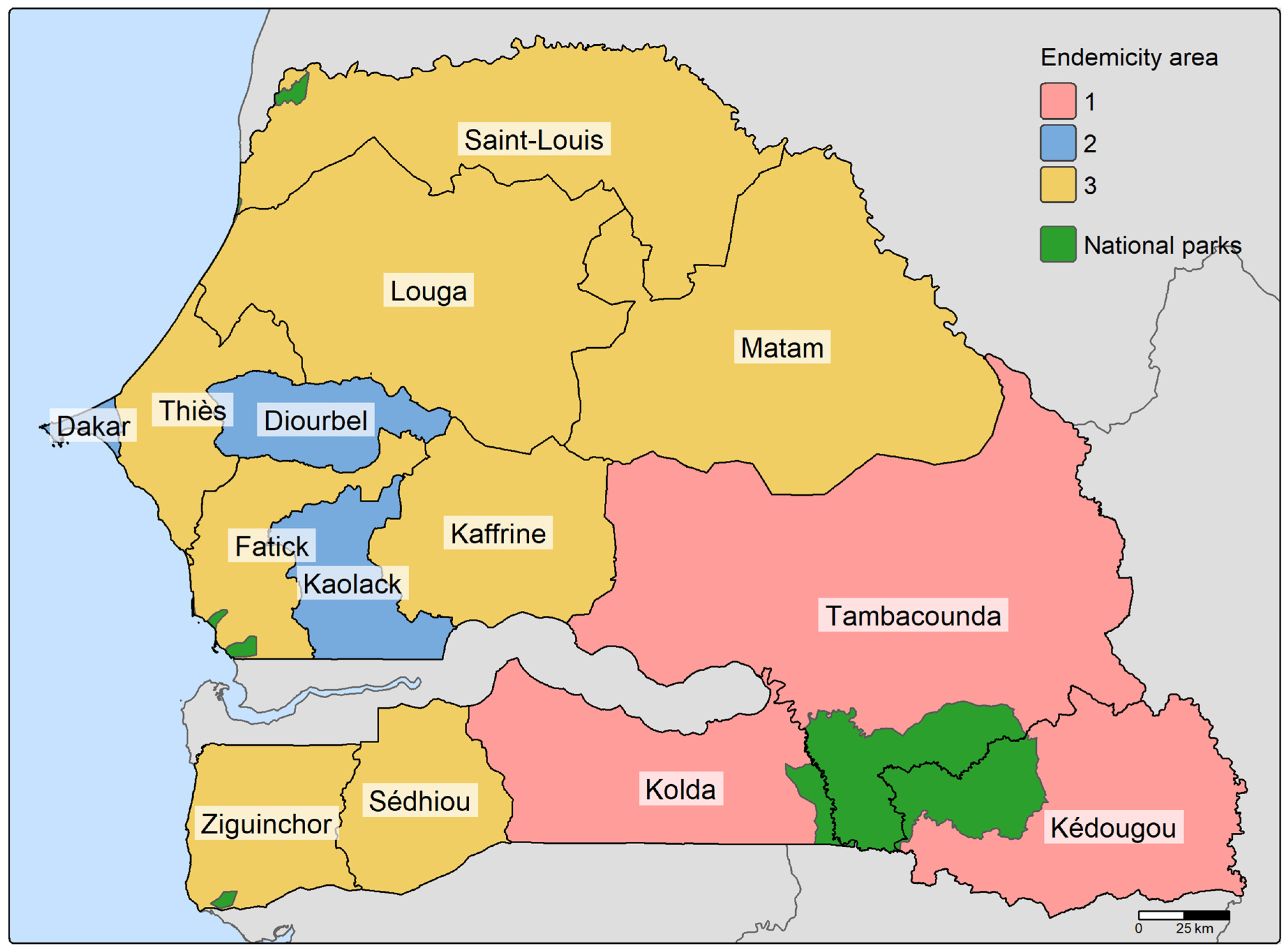
Figure 2.
Observed malaria incidence rates (MIR) (per 1,000 people) per health facility for 2017-2021. MIR were calculated using all annually reported cases.
Figure 2.
Observed malaria incidence rates (MIR) (per 1,000 people) per health facility for 2017-2021. MIR were calculated using all annually reported cases.
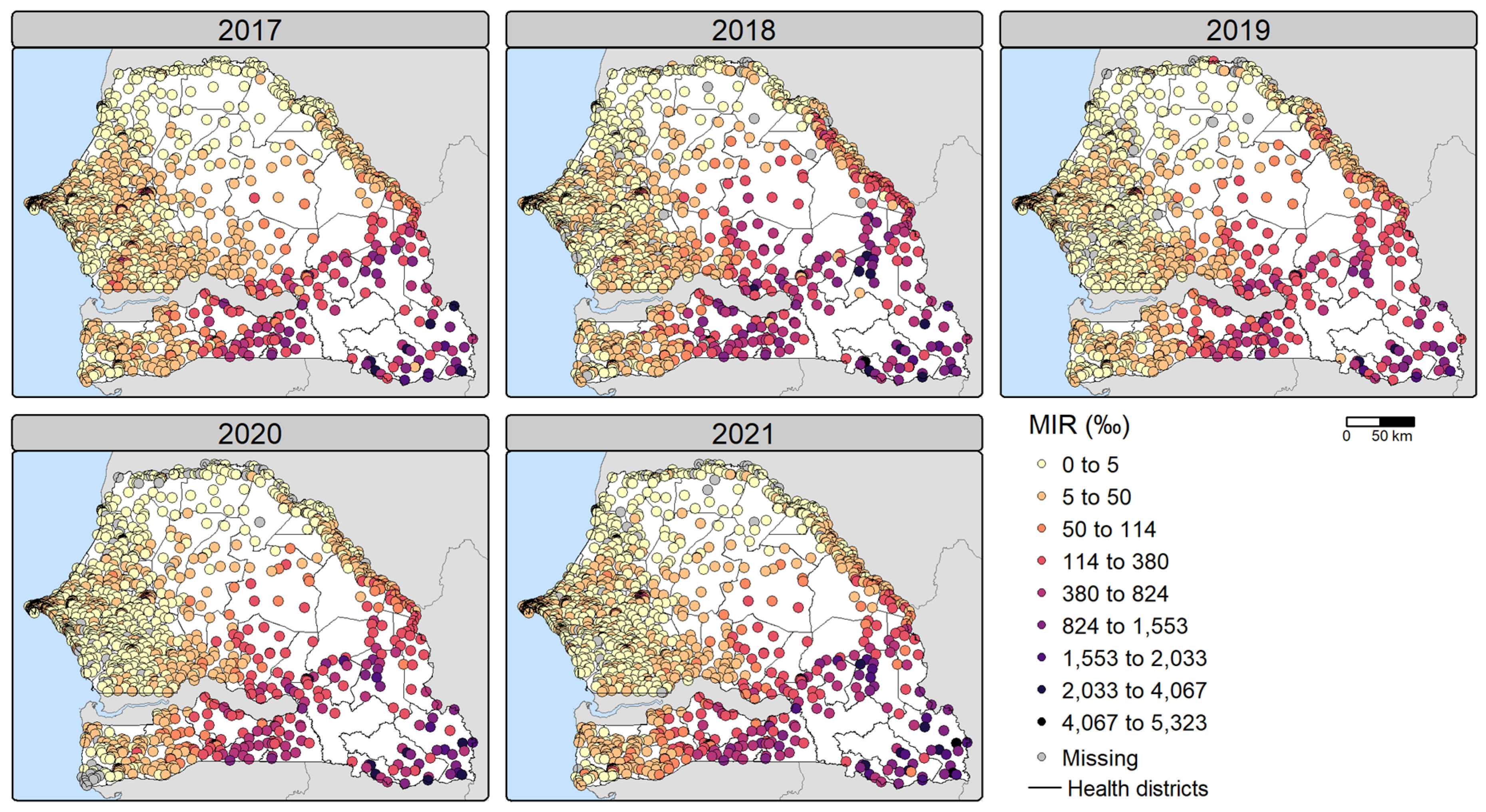
Figure 3.
Boxplot of malaria incidence rates (per 1,000 people) per health facility over 2017-2021. The middle horizontal line represents the median, while the dot represents the mean. Outliers are not shown to improve readability. Note that incidence rates above 1000‰ can be attributed to malaria repeat episodes [32] and migration. Abbreviations: KKT (Kolda, Kédougou, Tambacounda), E1 (endemicity 1), E2 (endemicity 2), E3 (endemicity 3).
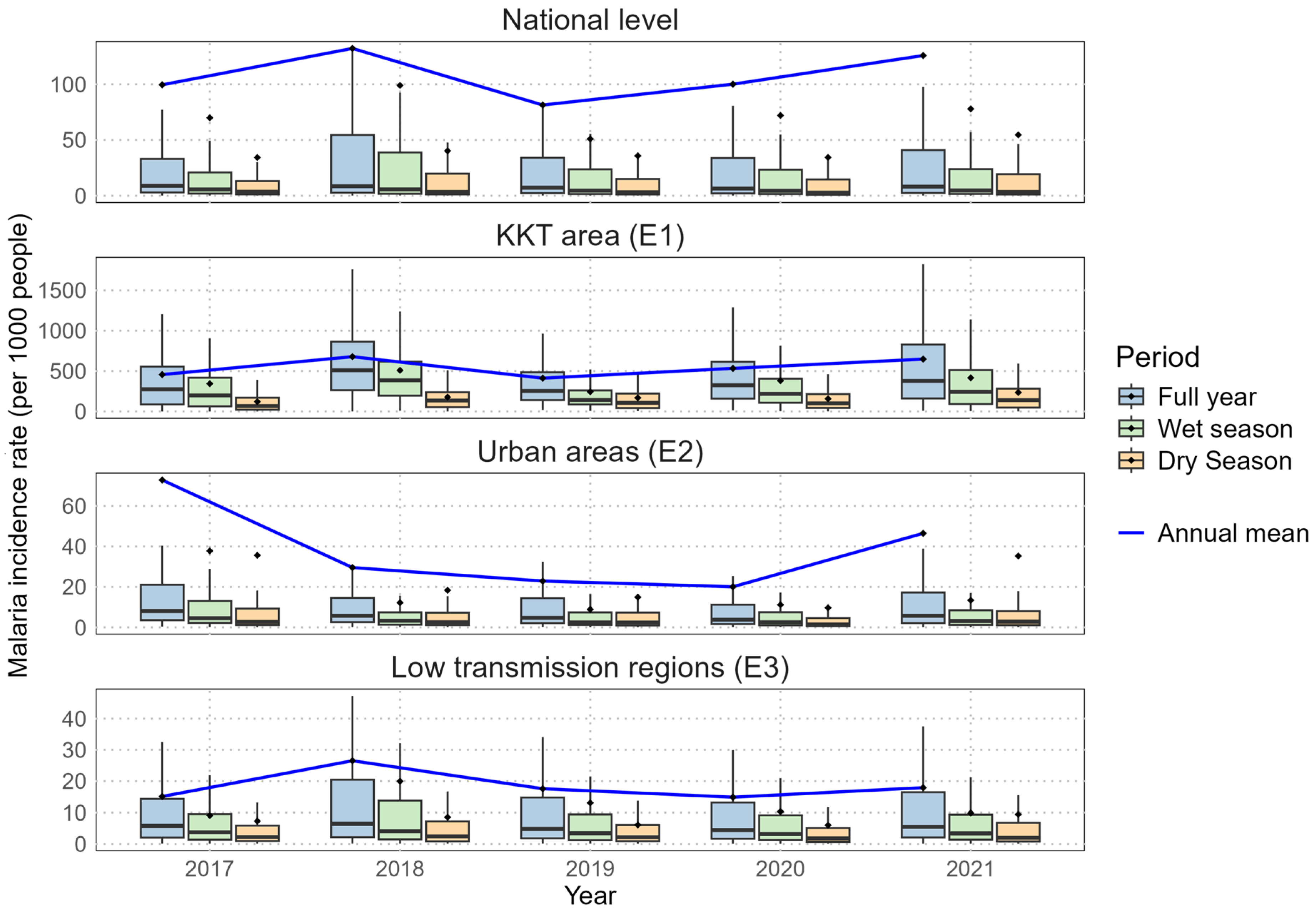
Figure 4.
Estimated malaria incidence rates (per 1,000 people) for 2017-2021 in Senegal by model. The number of cases per health facility was estimated by multiplying the posterior estimates (mean, 2.5th percentile and 97.5th percentile) of malaria incidence rate (MIR) per health facility by the total potential catchment population (i.e. assuming 100% of the population sought health care for fever). The total number of cases was summed and divided by the total population to calculate the annual MIR. The solid line represents the estimate based on the posterior mean MIR, while the shaded area is based on the posterior 2.5th and 97.5th percentile estimates. Note that the y-axis of the Endemicity 1 model estimates differs from the other models.
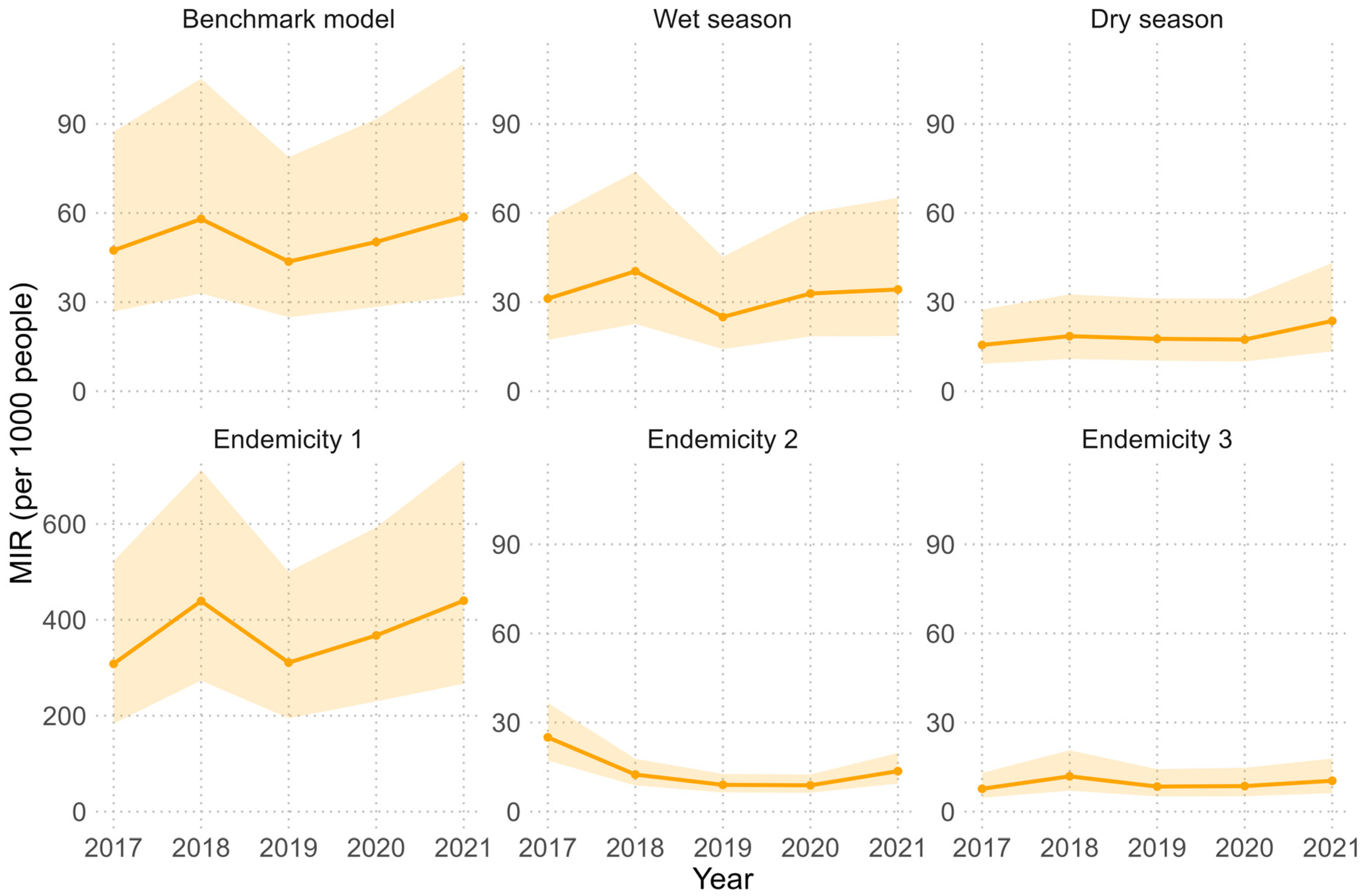
Figure 5.
Estimated malaria incidence rates (per 1,000 people) for 2017-2021 per health district. The number of cases per health facility was estimated by multiplying the posterior mean malaria incidence rate (MIR) per health facility by the total potential catchment population (i.e. assuming 100% of the population sought health care for fever). The total number of cases was summed per health district and divided by the total district population to calculate the MIR, which is then expressed per 1,000 people. These estimates are based on the benchmark model (BM). Note that incidence rates above 1000‰ can be attributed to malaria repeat episodes [32] and migration.
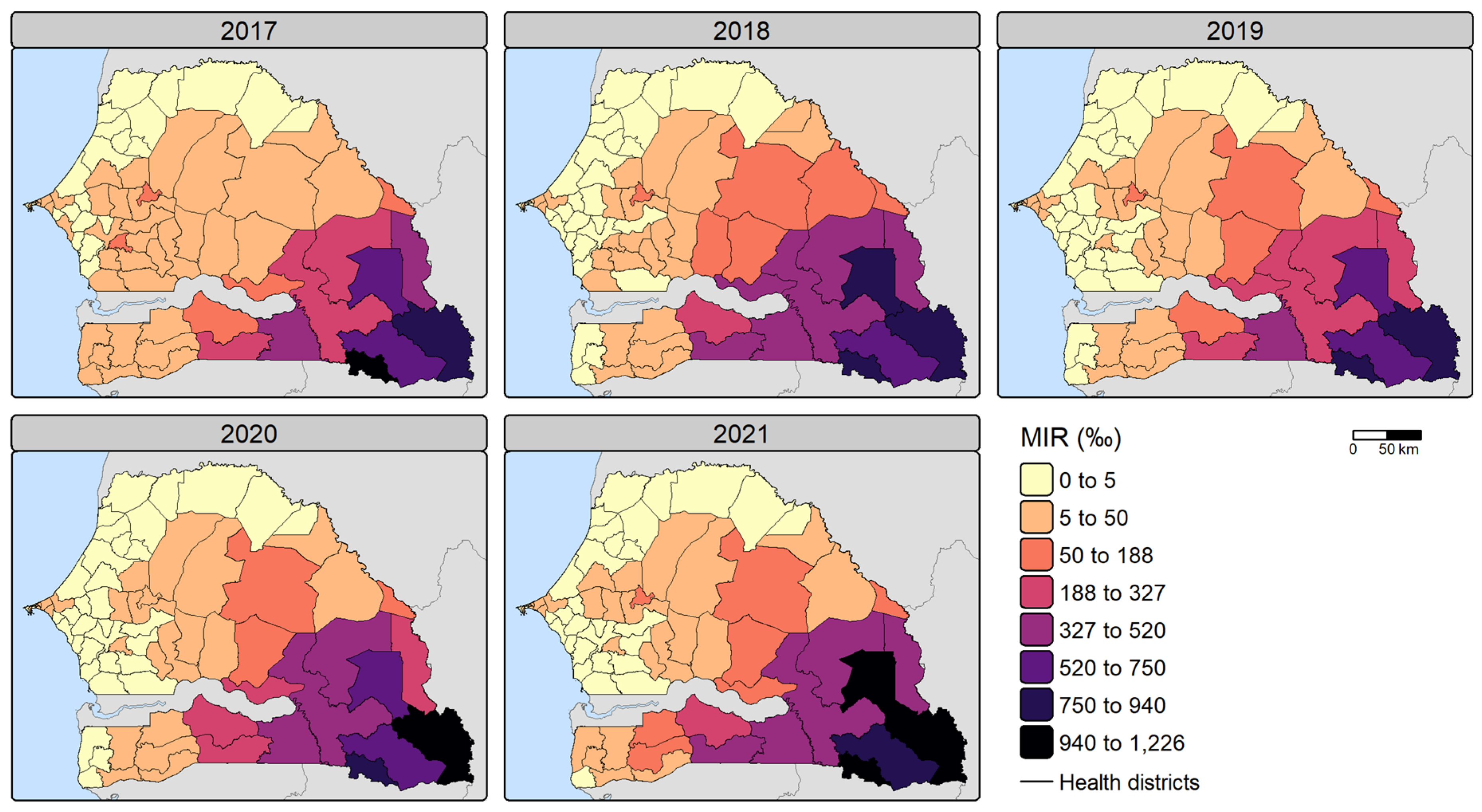
Figure 6.
Boxplot of performance metrics obtained by random cross-validation. The MAE, RMSE, R² and r² values were calculated on the test sets on the MIR scale after performing a random 5-repeated 5-fold cross-validation procedure. The R² is the coefficient of determination (COD) and the r² is the square of the correlation between the observed and predicted values. The middle horizontal line represents the median, while the dots represent outliers. Abbreviations: RMSE (root mean square error), MAE (mean absolute error), COD (coefficient of determination), BM (benchmark model), WM (wet season model), DM (dry season model), E1 (endemicity 1 model), E2 (endemicity 2 model), E3 (endemicity 3 model).
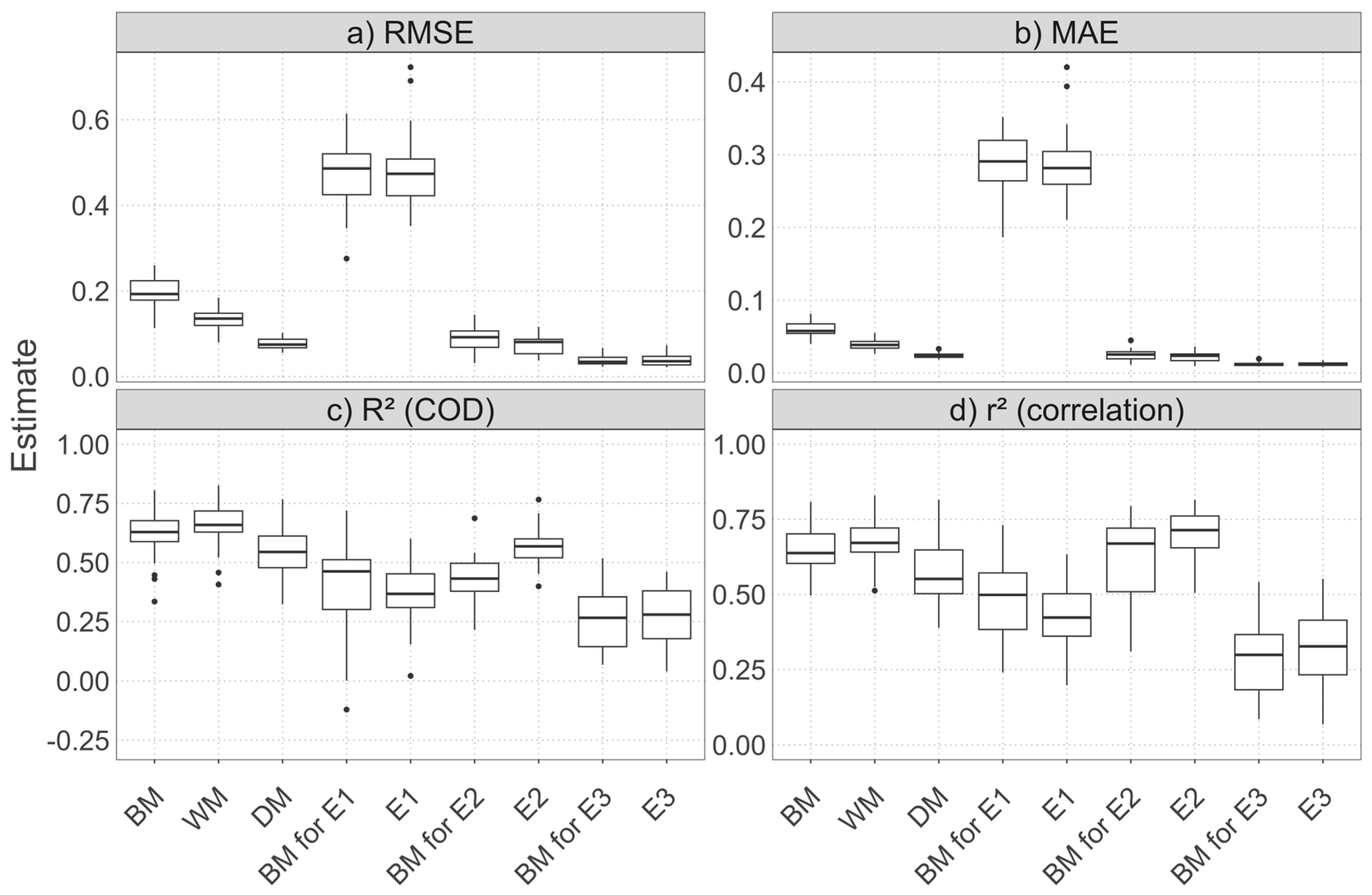
Figure 7.
Disaggregated reported malaria cases for 2017-2021 at 1x1 km resolution. The number of cases per pixel was obtained by a dasymetric disaggregation of the number of reported cases per health facility catchment area, using the posterior mean malaria incidence rate per pixel to compute the disaggregation weight. These estimates are based on the benchmark model.
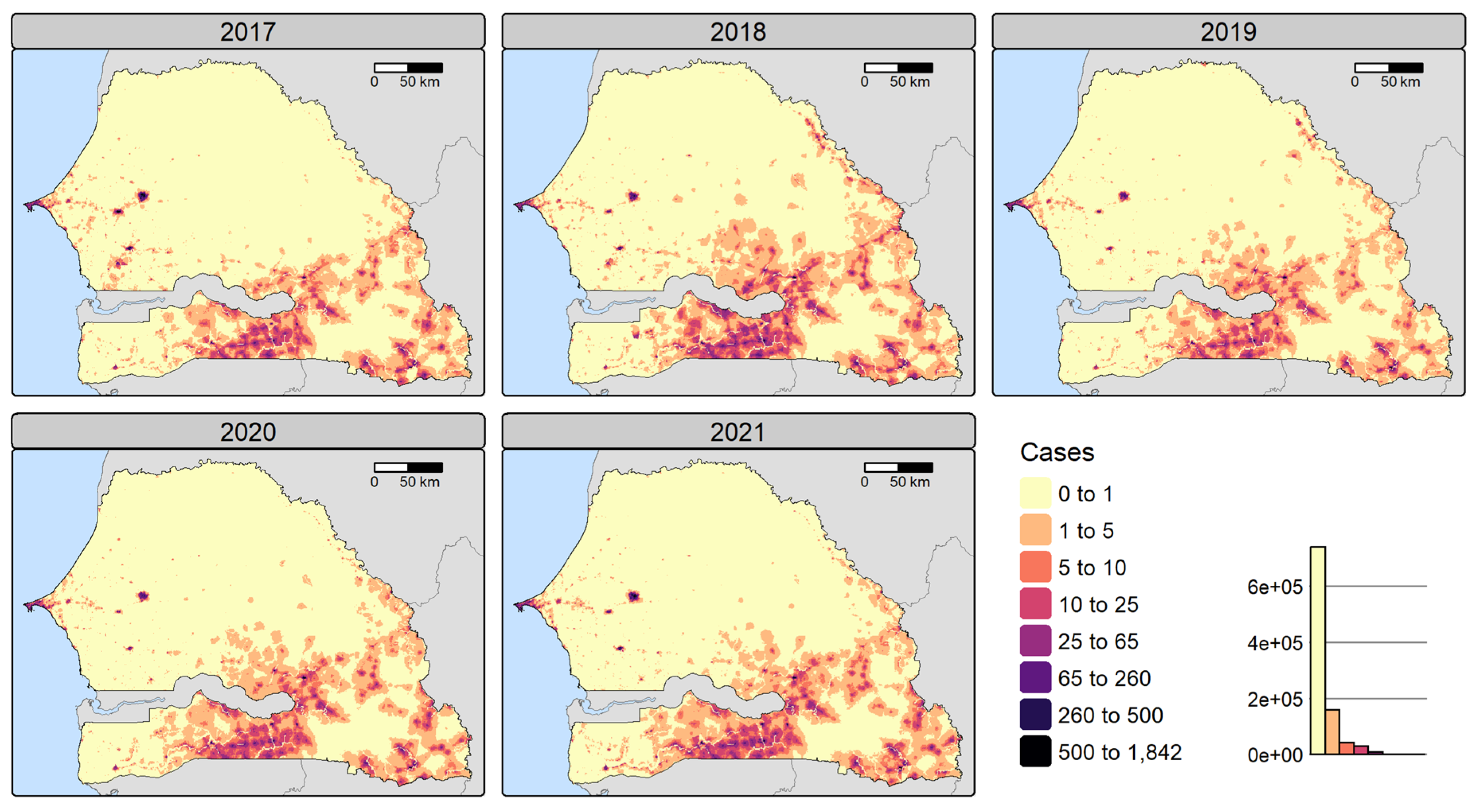
Figure 8.
Disaggregated malaria incidence rate (per 1,000 people) for 2017-2021 at 1x1 km resolution. Malaria incidence rates (MIR) were calculated by dividing the number of cases per pixel obtained by dasymetric disaggregation by the pixel treatment-seeking population. These estimates are based on the benchmark model. Note that incidence rates above 1000‰ can be attributed to malaria repeat episodes [32] and migration.
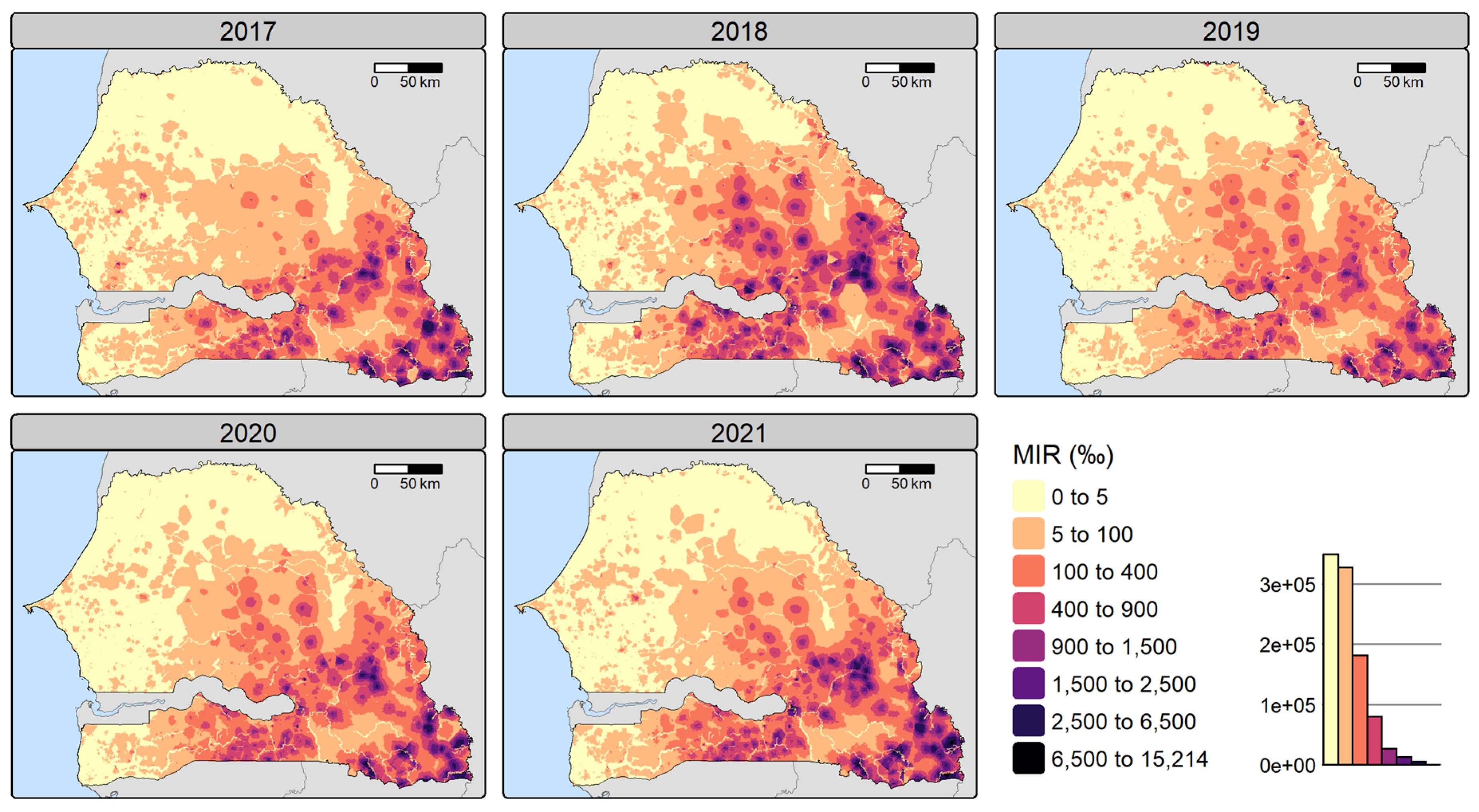

Table 1.
Geospatial covariates and their characteristics.
| Category | Variables | Date | Spatial resolution | Source |
| Climate & weather | Precipitation | Climatic average over 1988-2018 | 1000 m | CHELSA [54] (https://chelsa-climate.org/) |
| Day land surface temperature (LST), night LST | Annual (2017-2021) | 1000 m | MODIS [55,56] (http://modis.gsfc.nasa.gov/) | |
| Vector-habitat | Normalized difference moisture index (NDMI) | Annual (2017-2021) | 10 m | Computed from Sentinel-2 L1C composites of the Joint Research Centre (JRC) [57] (https://forobs.jrc.ec.europa.eu/sentinel/sentinel2_composite) |
| Land use and land cover: water, trees, flooded vegetation, cropland, grassland, bare land, shrubland, built-up | Annual (2017-2021) | 10 m | Dynamic World by Google and the World Resources Institute [58] (https://dynamicworld.app/) | |
| Elevation | 2000 | 30 m | US Geological Survey [59] (http://eros.usgs.gov/elevation-products) | |
| Susceptibility | Access to basic sanitation service, proportion of Fula, stunting in children | Annual (2017-19/20 avail.; stunting: 2020-21 proj., others: 2021 proj.) | Survey clusters | The DHS Program |
| Lack of resilience | Distance to major roads | 2023 | 100 m | OpenStreetMap (www.openstreetmap.org) |
| Walking-only travel time to health facilities | Annual (2017-2021) | 1000 m | Walking time is computed using elevation, land use, roads and rivers (see Section Computation of travel time) | |
| Ownership of insecticide-treated nets, literacy rate in women | Annual (2017-20 avail.; 2021 proj.) | Survey clusters | The DHS Program |
Note. Avail. and proj. stand for available and projected, respectively.
Table 2.
Land and road type and associated walking speed in km/h.
| Data source | Land and road type | Walking speed (km/h) |
| Dynamic World LULC | Built up | 5 |
| Trees | 3.5 | |
| Shrubland | 4.5 | |
| Cropland | 3.5 | |
| Grassland | 4 | |
| Bare ground | 5 | |
| Flooded vegetation | 0 | |
| Water bodies | 0 | |
| OpenStreetMap | Rivers | 0 |
| Roads | 5 |
Note. Walking speeds are based on [67]. LULC stands for land use land cover.
Table 3.
Model names and their descriptions.
| Model name | Description | Number of facilities |
| Benchmark model (BM) |
|
1472 (1389) |
| Wet season model (WM) |
|
1472 (1389) |
| Dry season model (DM) |
|
1472 (1389) |
| Endemicity 1 model (E1) |
|
217 (216) |
| Endemicity 2 model (E2) |
|
373 (328) |
| Endemicity 3 model (E3) |
|
882 (845) |
Note. is the number of malaria cases reported at facility in year . The number of health facilities in brackets reflects the number after merging cases of facilities within the same 1×1 km grid cell during catchment area extraction.
Table 4.
Covariates selected by Bayesian geostatistical models. .
| Category | Variable | BM | WM | DM | E1 | E2 | E3 | Number of models |
| Climate & weather | Precipitation | (⨯) | ⨯ | (⨯) | 3 | |||
| Day LST | ⨯ | ⨯ | ⨯ | ⨯ | 4 | |||
| Night LST | ⨯ | ⨯ | 2 | |||||
| Vector-habitat | NDMI | ⨯ | (⨯) | 2 | ||||
| Prop. of bare land | (⨯) | ⨯ | ⨯ | 3 | ||||
| Prop. of built-up | ⨯ | ⨯ | ⨯ | ⨯ | ⨯ | ⨯ | 6 | |
| Prop. of cropland | (⨯) | (⨯) | ⨯ | 3 | ||||
| Prop. of flooded vegetation | ⨯ | (⨯) | 2 | |||||
| Prop. of shrubland | ⨯ | ⨯ | 2 | |||||
| Prop. of trees | ⨯ | ⨯ | 2 | |||||
| Prop. of water | ⨯ | 1 | ||||||
| Elevation | ⨯ | ⨯ | 2 | |||||
| Susceptibility | Access to basic sanitation | ⨯ | ⨯ | ⨯ | ⨯ | 4 | ||
| Prop. of Fula | ⨯ | 1 | ||||||
| Stunting in children | ⨯ | ⨯ | ⨯ | ⨯ | ⨯ | ⨯ | 6 | |
| Lack of resilience | Distance to major roads | ⨯ | ⨯ | ⨯ | ⨯ | 4 | ||
| Walking time to health facilities | ⨯ | ⨯ | ⨯ | ⨯ | ⨯ | ⨯ | 6 | |
| Number of covariates | 9 | 10 | 8 | 9 | 9 | 8 | / |
Note. Covariate selection was performed using a forward stepwise variable selection (with the INLAstep function from the INLAutils package). A cross indicates that the covariate was included in the model, while brackets indicate that the covariate is not statistically significant based on the 95% credible intervals. Underlined covariates were selected by all models. Covariates not selected by any model are not shown. Abbreviations: BM (benchmark model), WM (wet season model), DM (dry season model), E1 (endemicity 1 model), E2 (endemicity 2 model), E3 (endemicity 3 model), LST (land surface temperature), prop. (proportion). .
Table 5.
Posterior estimates of the benchmark model and models stratified by season.
| Variable | Benchmark (BM) | Wet season (WM) | Dry season (DM) | ||||||
| Mean | 2.5% quant. | 97.5% quant. | Mean | 2.5% quant. | 97.5% quant. | Mean | 2.5% quant. | 97.5% quant. | |
| ) | -3.61 | -4.40 | -2.82 | -4.00 | -4.72 | -3.28 | -4.37 | -5.12 | -3.62 |
| Day LST | -0.37 | -0.50 | -0.23 | -0.34 | -0.48 | -0.19 | - | - | - |
| Night LST | 0.26 | 0.15 | 0.37 | 0.24 | 0.13 | 0.36 | - | - | - |
| Prop. of bare land | - | - | - | 0.003 | -0.08 | 0.07 | - | - | - |
| Prop. of built-up | 0.57 | 0.52 | 0.62 | 0.51 | 0.44 | 0.58 | 0.63 | 0.58 | 0.67 |
| Prop. of cropland | 0.02 | -0.03 | 0.07 | - | - | - | 0.04 | -0.01 | 0.10 |
| Prop. of flooded vegetation | - | - | - | -0.10 | -0.16 | -0.05 | - | - | - |
| Prop. of shrubland | - | - | - | -0.11 | -0.19 | -0.02 | - | - | - |
| Prop. of trees | 0.11 | 0.05 | 0.17 | - | - | - | 0.15 | 0.09 | 0.22 |
| Elevation | - | - | - | - | - | - | -0.13 | -0.23 | -0.03 |
| Access to basic sanitation | 0.23 | 0.16 | 0.30 | 0.25 | 0.18 | 0.32 | 0.18 | 0.11 | 0.25 |
| Stunting in children | 0.26 | 0.17 | 0.35 | 0.29 | 0.20 | 0.37 | 0.25 | 0.16 | 0.33 |
| Distance to major roads | -0.19 | -0.25 | -0.13 | -0.12 | -0.18 | -0.06 | -0.13 | -0.19 | -0.07 |
| Walking time to health facilities | -0.35 | -0.41 | -0.28 | -0.34 | -0.41 | -0.28 | -0.38 | -0.45 | -0.31 |
| Precision of uncorrelated random variations ( | 1.12 | 1.08 | 1.17 | 1.17 | 1.13 | 1.22 | 1.09 | 1.05 | 1.13 |
| ) | 2.16a | 1.71 | 2.73 | 2.22b | 1.74 | 2.76 | 2.01c | 1.59 | 2.53 |
| SD of spatially correlated variations ( | 2.78 | 2.22 | 3.46 | 2.53 | 2.00 | 3.10 | 2.57 | 2.06 | 3.19 |
| ) | 0.99 | 0.98 | 0.99 | 0.98 | 0.97 | 0.99 | 0.99 | 0.98 | 0.99 |
Note. a,b,c These correspond to a range of approximately 240, 247 and 223 km respectively (1° = 111.12 km). The quantiles are obtained by taking the 95% credible intervals of the posterior estimates. Abbreviations: LST (land surface temperature), prop. (proportion), SD (standard deviation).
Table 6.
Posterior estimates of the models stratified by endemicity level. .
| Variable | Endemicity 1 | Endemicity 2 | Endemicity 3 | ||||||
| Mean | 2.5% quant. | 97.5% quant. | Mean | 2.5% quant. | 97.5% quant. | Mean | 2.5% quant. | 97.5% quant. | |
| ) | -1.24 | -2.20 | -0.32 | -5.98 | -7.24 | -4.72 | -4.56 | -5.44 | -3.67 |
| Precipitation | 0.45 | -0.06 | 0.96 | 1.64 | 0.95 | 2.34 | 0.17 | -0.05 | 0.38 |
| Day LST | -1.60 | -2.08 | -1.12 | - | - | - | -0.14 | -0.26 | -0.02 |
| NDMI | -0.50 | -0.70 | -0.30 | 0.17 | -0.08 | 0.42 | - | - | - |
| Prop. of bare land | - | - | - | 0.22 | 0.09 | 0.35 | -0.08 | -0.15 | -0.02 |
| Prop. of built-up | 0.43 | 0.28 | 0.58 | 0.63 | 0.52 | 0.75 | 0.53 | 0.46 | 0.60 |
| Prop. of cropland | - | - | - | 0.35 | 0.20 | 0.50 | - | - | - |
| Prop. of flooded vegetation | 1.15 | -0.22 | 2.53 | - | - | - | - | - | - |
| Prop. of shrubland | -0.38 | -0.50 | -0.26 | - | - | - | - | - | - |
| Prop. of water | -1.23 | -1.76 | -0.69 | - | - | - | - | - | - |
| Elevation | - | - | - | -0.58 | -0.95 | -0.21 | - | - | - |
| Access to basic sanitation | - | - | - | - | - | - | 0.18 | 0.09 | 0.27 |
| Prop. of Fula | - | - | - | -0.31 | -0.59 | -0.04 | - | - | - |
| Stunting in children | 0.40 | 0.26 | 0.54 | 0.32 | 0.09 | 0.54 | 0.25 | 0.14 | 0.37 |
| Distance to major roads | - | - | - | - | - | - | -0.21 | -0.28 | -0.14 |
| Walking time to health facilities | -0.23 | -0.30 | -0.16 | -1.84 | -2.17 | -1.51 | -0.36 | -0.45 | -0.27 |
| Precision of uncorrelated random variations ( | 2.27 | 2.05 | 2.50 | 1.02 | 0.95 | 1.10 | 1.15 | 1.09 | 1.20 |
| ) | 1.74a | 1.13 | 2.57 | 0.91b | 0.59 | 1.40 | 2.17c | 1.59 | 2.87 |
| SD of spatially correlated variations ( | 1.58 | 1.10 | 2.21 | 1.80 | 1.31 | 2.46 | 2.46 | 1.83 | 3.21 |
| ) | 0.97 | 0.95 | 0.99 | 0.97 | 0.94 | 0.99 | 0.98 | 0.96 | 0.99 |
Note. a,b,c These correspond to a range of approximately 193, 101 and 241 km respectively (1° = 111.12 km). The quantiles are obtained by taking the 95% credible intervals of the posterior estimates. Abbreviations: LST (land surface temperature), prop. (proportion), SD (standard deviation).
Table 7.
Mean performance metrics (MAE, RMSE, R² and r²) obtained by cross-validation (MIR scale). .
Table 7.
Mean performance metrics (MAE, RMSE, R² and r²) obtained by cross-validation (MIR scale). .
| Random CV | RMSE | MAE | R² (COD) | r² (corr.) |
| Benchmark (BM) | 0.20 | 0.06 | 0.62 | 0.65 |
| BM for E1 | 0.47 | 0.29 | 0.40 | 0.48 |
| BM for E2 | 0.09 | 0.03 | 0.43 | 0.60 |
| BM for E3 | 0.04 | 0.01 | 0.26 | 0.29 |
| Wet season (WM) | 0.13 | 0.04 | 0.65 | 0.67 |
| Dry season (DM) | 0.08 | 0.02 | 0.54 | 0.56 |
| Endemicity 1 (E1) | 0.48 | 0.29 | 0.37 | 0.43 |
| Endemicity 2 (E2) | 0.08 | 0.02 | 0.57 | 0.69 |
| Endemicity 3 (E3) | 0.04 | 0.01 | 0.27 | 0.32 |
| Temporal block CV | RMSE | MAE | R² (COD) | r² (corr.) |
| Benchmark (BM) | 0.17 | 0.05 | 0.70 | 0.75 |
| BM for E1 | 0.41 | 0.25 | 0.55 | 0.65 |
| BM for E2 | 0.09 | 0.03 | 0.44 | 0.63 |
| BM for E3 | 0.04 | 0.01 | 0.19 | 0.30 |
| Wet season (WM) | 0.13 | 0.04 | 0.66 | 0.77 |
| Dry season (DM) | 0.07 | 0.02 | 0.63 | 0.66 |
| Endemicity 1 (E1) | 0.41 | 0.24 | 0.55 | 0.64 |
| Endemicity 2 (E2) | 0.08 | 0.03 | 0.49 | 0.68 |
| Endemicity 3 (E3) | 0.04 | 0.01 | 0.20 | 0.31 |
Note. The MAE, RMSE, R² and r² values were calculated on the cross-validation test sets using the exponentiated posterior means of log MIR. The R² is the coefficient of determination (COD) and the r² is the square of the correlation between the observed and predicted values. BM for E1, BM for E2 and BM for E3 refer to the performance of the benchmark model (BM) within endemicity areas 1, 2 and 3. Abbreviations: CV (cross-validation), MAE (mean absolute error), RMSE (root mean square error), COD (coefficient of determination), corr. (correlation), MIR (malaria incidence rate).
Disclaimer/Publisher’s Note: The statements, opinions and data contained in all publications are solely those of the individual author(s) and contributor(s) and not of MDPI and/or the editor(s). MDPI and/or the editor(s) disclaim responsibility for any injury to people or property resulting from any ideas, methods, instructions or products referred to in the content. |
© 2025 by the authors. Licensee MDPI, Basel, Switzerland. This article is an open access article distributed under the terms and conditions of the Creative Commons Attribution (CC BY) license (http://creativecommons.org/licenses/by/4.0/).
Copyright: This open access article is published under a Creative Commons CC BY 4.0 license, which permit the free download, distribution, and reuse, provided that the author and preprint are cited in any reuse.


