Submitted:
06 June 2025
Posted:
09 June 2025
You are already at the latest version
Abstract
Ground Penetrating Radar surveys on structures have a wide range of application and they are very useful in solving engineering problems: from detecting reinforcement, studying concrete characteristics, unfilled joints, analyzing brick elements, detecting water content in building bodies, and evaluating structural deformation. They generally pursued small investigation areas with measurements made in direct contact with target structures and for small depths. In this paper we are illustrating an exploration on plinth foundations, supported by drilled piles, submerged in soil, extensive, deep and uninformed. Pulse GPR prospecting was performed in common-offset and single-fold, bistatic configuration, exploiting the exposed faces of an excavation around the foundation. In addition, 3 velocity tests were conducted including 2 in common mid-point and one in zero-offset transillumination in order to explore the range of variation of relative dielectric permittivity in the investigated media. The electromagnetic back-scattering analysis approach allowed us to extract the weighted average frequency attribute section. In it, anomalies emerge on the presence of drilled piles with 4 15 piles with an estimated diameter of 80 cm.
Keywords:
ground penetrating radar
; pile
; common mid point
; transillumination
; plynth
; back scattering field analisys
; weighted average frequency
; signal attributes
1. Introduction
The study described in here fits into the broad field of applications of Ground Penetrating Radar (GPR) and in particular that of man-made structures. The recents developments [1] in the methods of acquisition, data processing [2] and presentation of results have strengthened a toughter confidence in the use of this tool [3,4]. GPR has been successfully used to study beams, columns, slabs, bridges, tunnels, reinforcing bars, cracks and cracking in concrete, subsidence, stratigraphy, voids and cavities and foundations [5,6,7]. We describe a method of geophysical prospecting on bored piles, the verification of their number, and estimation of their geometry under extended foundations on plinth, on which they are constrained, under abutment foundation. The prospecting was carried out in May 2023 at the Liscione Bridge, built between 1967 and 1974, in the Monte Arcano district, on the SS 647 Biferno valley floor, in the province of Campobasso, Molise. An excavation carried out adjacent to an abutment, functional for the maintenance of the drainage around the foundation, uncovered the plinth and surrounding soil and provided a unique opportunity to access the seabed walls and verify the presence and quantity of piles drilled below the plinth. The work done is important because it allows us to shed light on relatively recent man-made structures for which design drawings are no longer available. Indirectly investigating, with geophysical methods, the bored piles below the foundations is difficult from the ground surface, especially if the depth between the head of the piles and the ground level is considerable, as in this case, which is 4 m. GPR studies of this kind are very recent [5,8] and the need for extraordinary maintenance for aging civil works is giving a boost to prospecting and research with GPR aimed at these applications.
2. Materials and Methods
Ground-penetrating radar detects dielectric discontinuities and hence makes it possible to investigate objects that are buried in visually opaque media. The dielectric wave has a lot of information which can be related to the parameters significant to hydrology, soil mechanics, and material property characterizations [9]. Moreover, the dielectric wave also efficient for quantified the properties of the host materials and the nature and size of the superficial bodies as well [10]. The method is based in the transmission of electromagnetic waves through the subsurface to characterize terrains with changes in their electromagnetic properties. The electromagnetic wave propagation is governed by Maxwell’s equations [11]. The way that GPR responds to each material is governed by two physical properties of the material: electrical conductivity and dielectric constant. The dielectric contrast is a descriptive number that indicates, among other things, how fast radar energy travels through a material. In materials of low magnetic susceptibility, velocity and attenuation are related to the Relative Dielectric Permettivity (RDP) and loss tangent, , by the expressions [12]
where is the angular frequency, f is the frequency and c is the velocity of the EM wave in the empty space (30 cm/ns). There are some main parameter to define for common-offet, single fold pulse radar reflextion survey [13].
Operating frequency: a simple rule of thumb for your choice is
where f is the operating frequency, z is the required depth of investigation;
time window:
sampling interval:
where t is the time in ns and f is the center frequency in Mhz;
resolution: can be taken as one-quarter of the wavelength [14] of EM wave [15]
where t is the time in ns and f is the center frequency in Mhz;
radius of footprint of the elliptical illumination cone of GPR into the ground is [16]
where is the center frequency wavelength of EM wave, D is the depth from the ground surface to the reflection surface, is the relative dielectric permettivity of material from the ground to the surface depth (D).
At the investigated site, the pulsed GPR geophysical prospecting method was used to obtain high-resolution subsurface information. It, with broadband antennas transmits electromagnetic waves that are received by others to obtain radargrams [11], which allow studying anomalies generated by objects or contrasts in geophysical parameters such as relative dielectric permittivity (), electrical conductivity (). In pulsed GPR, the shape of the transmitted pulse is calibrated to obtain a Gaussian-type spectral distribution [14] where the central value represents the characteristic frequency of the antenna, which corresponds to the dominant frequency of the pulse. It determines the resolution and the maximum exploration depth characteristics. The working hypothesis is based on the question of whether it is possible to reveal the presence of bored piles hidden by a plinth and surrounding soil with GPR. The use of common-offset and single fold scans, on the sides of each exposed face of the foundation, could show anomalies if there are contrasts in dielectric permittivity and/or electrical conductivity [12]. To verify this, first we need to explore the site-specific relationship between these variables, depending on the spatial geometry and acquisition method [17]. The sediments encompassing the piles were wet, and we know that the permittivity and conductivity of rocks and soils depend in a large extent on their water content [18]. Both permittivity and conductivity also depend on other properties of the investigated material, in particular on its porosity and clay content, such that the application of such empirical laws should be site- and scale-dependent [19]. The influence of electrical conductivity can only be neglected in dry soils that do not contain clay particles. GPR data are mostly sensitive to permittivity and much less to conductivity [20]. If the contrasts associated with these parameters are weak then the study of the electromagnetic signal and its attributes will be necessary [21].
2.1. Geometry of the Site, B-Scans, and GPR Velocity Tests
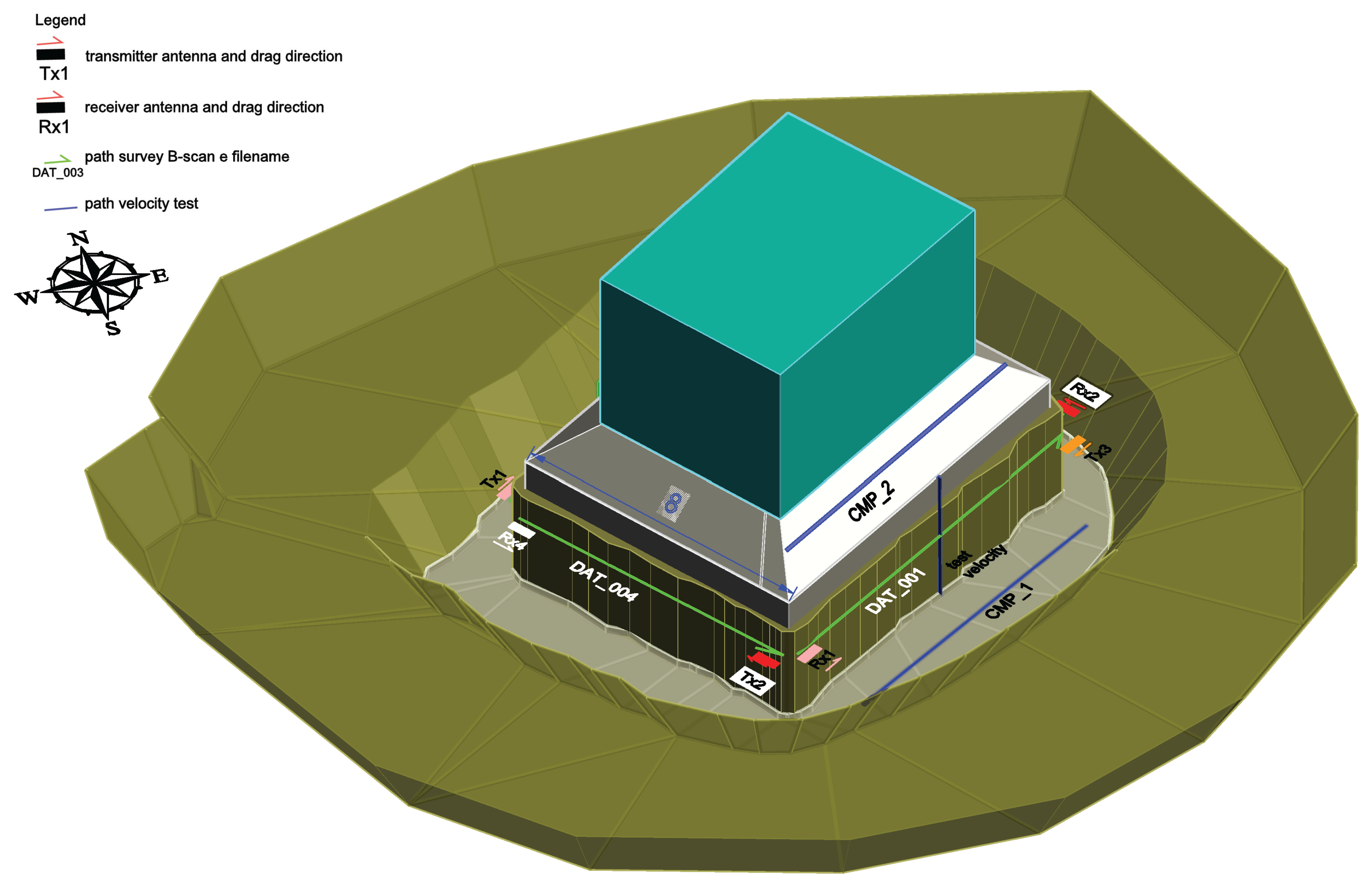
In situ, the bridge pylon rests on a trapezoidal plinth. The plinth in turn is constrained to deep bored piles. Geologically, the area insists on upper Pleistocene terraced alluvial soils. The lithologies are mixed-grained: silt, sand, clay, and gravel in varying proportions with the sandy component prevailing; moisture in the exposed soils was evident. The plinth was 10 m long, 8 m wide and 2.3 m high, while the underlying soil was 1.3 m thick to the bottom of the excavation. The base of the plinth was at a depth of about 4 m above the ground level.
Figure 1.
3D view of the site: the stations of the 2 CMP tests, the transillumination test and the 4-sided B-scans are shown with the location of the transmitting and receiving antennas, for each acquisition, drag direction and filename.
Figure 1.
3D view of the site: the stations of the 2 CMP tests, the transillumination test and the 4-sided B-scans are shown with the location of the transmitting and receiving antennas, for each acquisition, drag direction and filename.
2.2. GPR Instrumentation and Acquisition Parameters
The survey was carried out in the spring using a radar system from “Radar System Inc.” with a time range up to 2000 nsec, frequency of pulse repetition of transmitter 115 KHz, 320 scans per second, 1024 samples per scan and staking of traces up to 128. The antennas used, separately that transmitter and receiver, are the 200 Mhz, 300 Mhz and 500 Mhz and a connecting cable of length 30 m. The antennas are bow-tie, ground coupled, shielded type.
Figure 2.
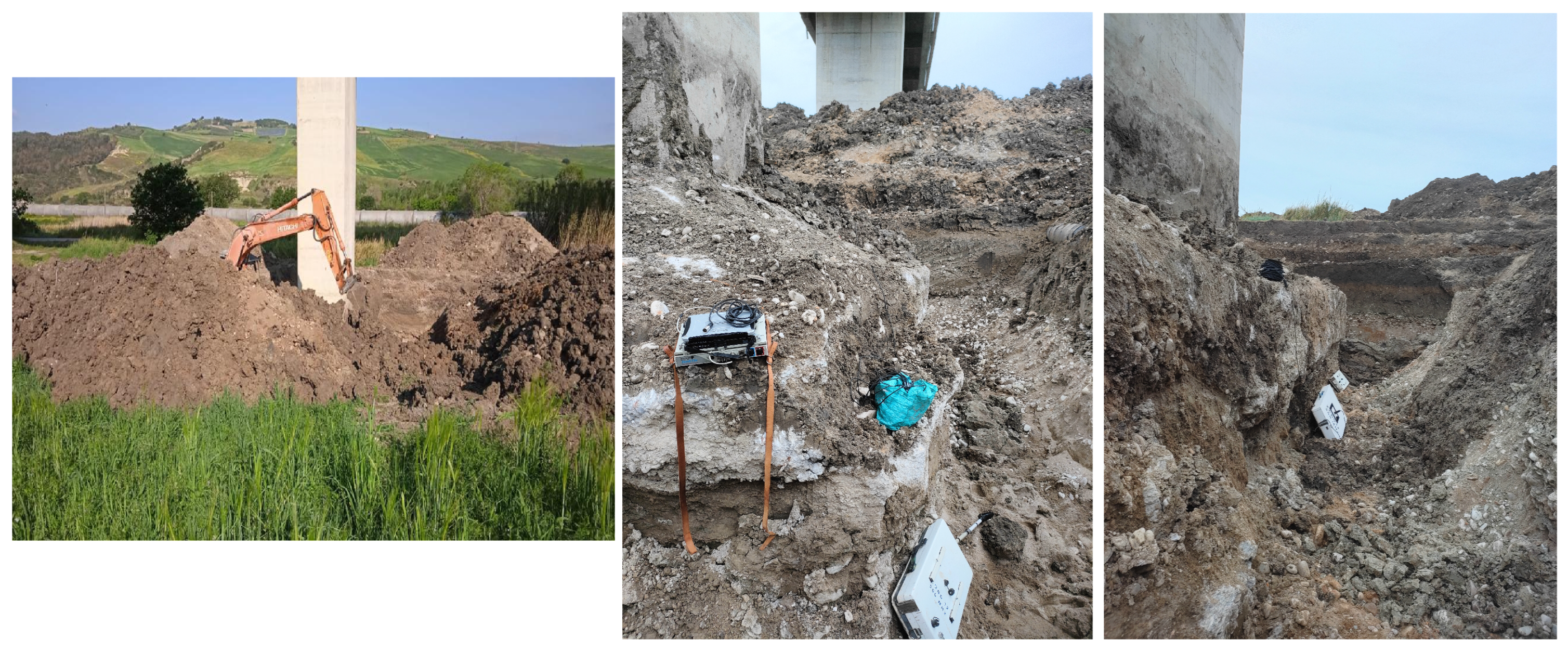
Excavation of the foundation for drainage maintenance and acquisition steps with the antennas, control unit, connection cable reel.
Figure 2.
Excavation of the foundation for drainage maintenance and acquisition steps with the antennas, control unit, connection cable reel.
GPR raw data were processed using PRISM (radsys.lv), Georadar-Expert (gpr-soft.com), Matlab (mathworks.com), Seismic Unix (wiki.seismic-unix.org). This combination of tools enabled sophisticated data analysis and visualization, enhancing the quality of the survey results. Preliminarily, the propagation of the electromagnetic wave was simulated qualitatively in time domain to understand how different center frequency antennas could perform, as well as getting an idea of how the A-scan might look like in the given conditions [22]. The positioning was done with metric measurements of the entire site and plinth geometry in order to obtain a 3D reconstruction. The scans were measured and marked using some spray references.
2.3. Direct In Situ Velocity Tests: CMP and Zero-Offset Transillumination
For the calibration of the propagation speed of the electromagnetic wave in the medium, the following in situ velocity tests had to be carried out:
- 1 test Common Mid Point on the excavated bottom
- 1 test Common Mid Point on the exposed plinth
- 1 test transillumination zero-offset on the two faces of the short side of the foundation.
The two CMPs were performed by symmetrically moving 2 antennas with a constant step, a 500 Mhz transmitter and a 300 Mhz receiver, along the same direction and each in opposite direction starting from a common midpoint. The CMP method is suitable for building structures [23].
Figure 3.
Geometry of the acquisition area, CMP tests, and zero-offset transillumination.
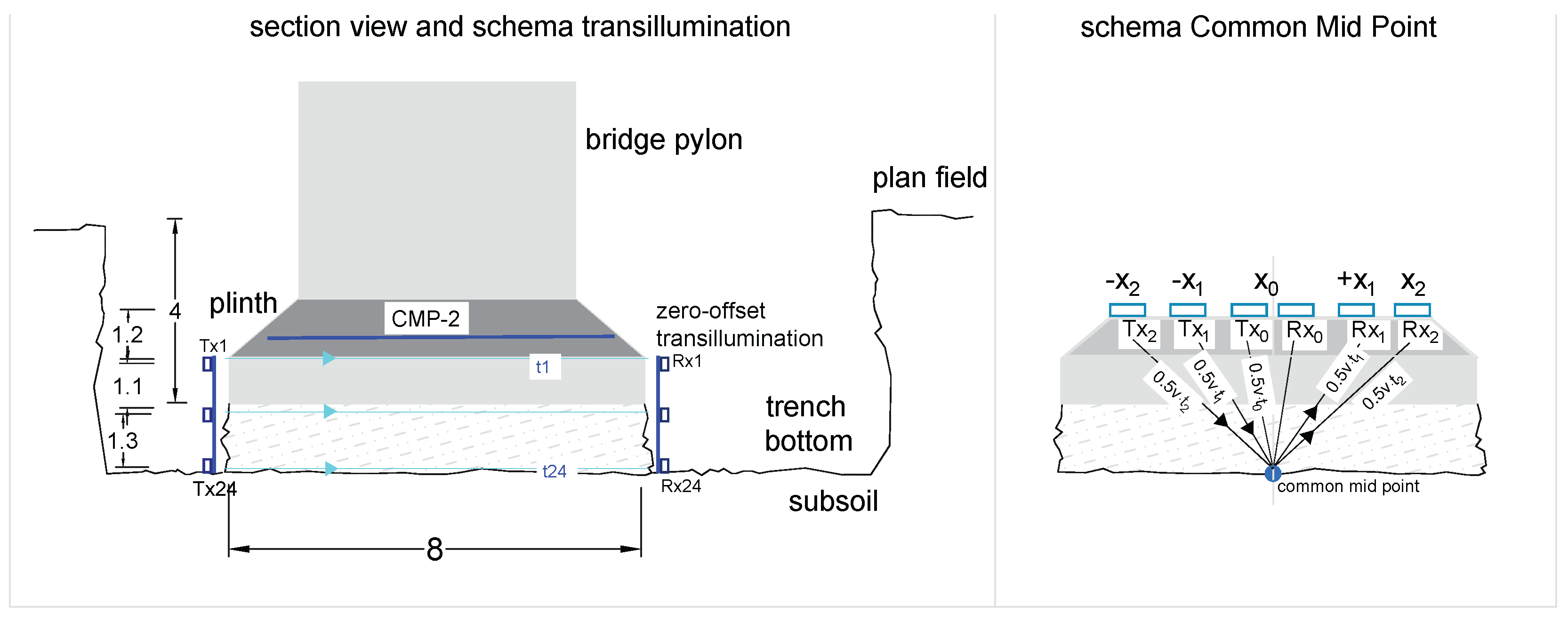
In the CMP test since the signal path length is symmetrical to the vertical axis (crossing), the travel time of the electromagnetic wave, between transmitter and receiver, is simply halved. To determine the velocity in the crossed medium and so the relative permittivity, the following trigonometric relation can be applied:
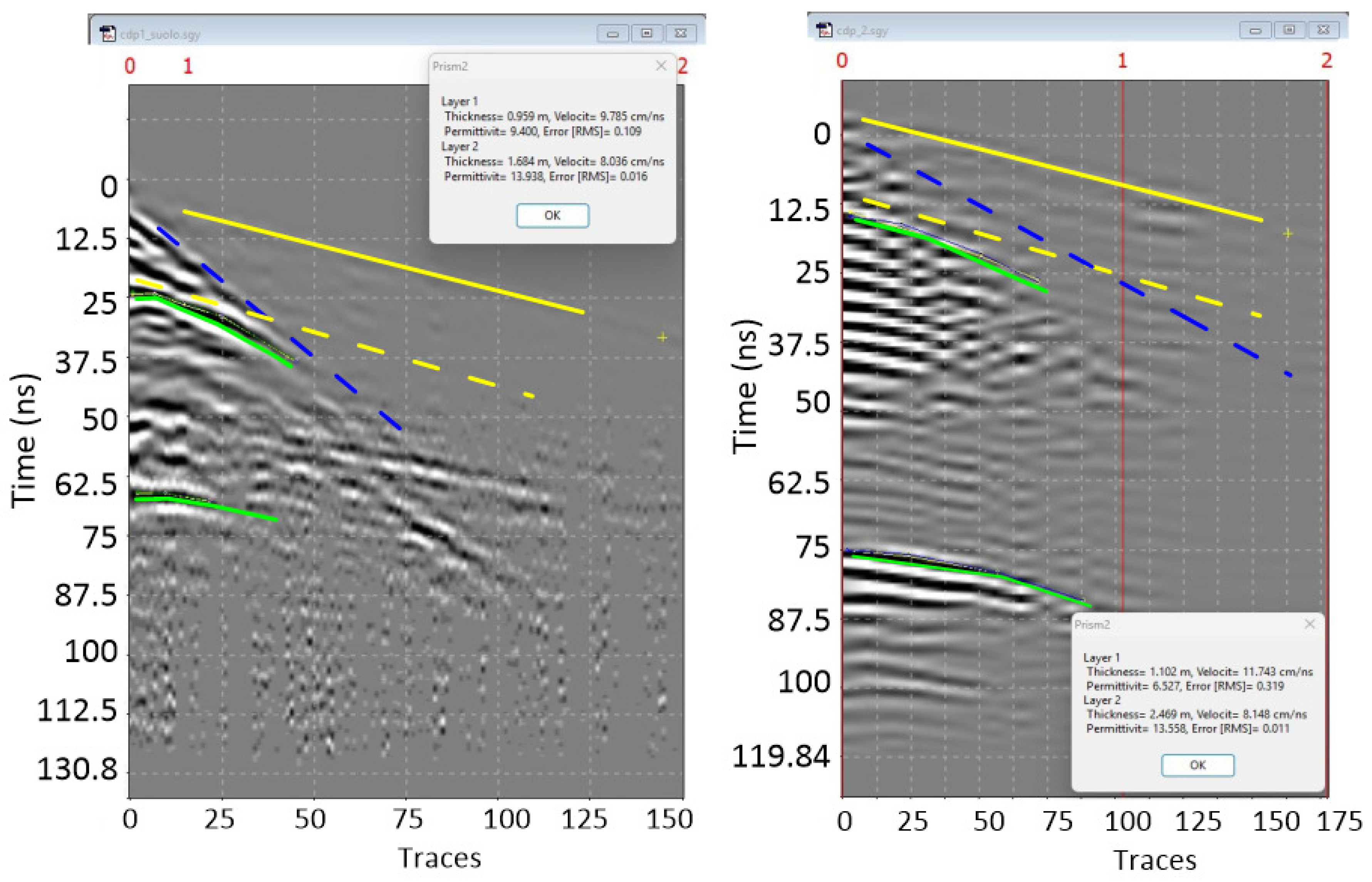
where: the time of flight of the signal is the time the signal needs from the transmitter and back to the receiver, while is the time to and from the target at the coordinate of the minimum distance (). The advantage of the CMP test is that the receiver does not become saturated while receiving the reflected signal [23]. The radargrams of the CMP acquisitions can be seen in the following figure, where the free air wave has been highlighted with the solid yellow line, the dashed yellow line instead the critically refracted air wave, the blue dashed line the ground wave and the lines in green the refracted waves. In the gray box of each are calculated the results of the velocities and permittivities, shown in detail in Table 3.
Figure 4.
CMP1 radargrams on the left and CMP2 on the right.
The zero-offset transillumination test between the transmitting and receiving antennas was possible by having 4 vertical faces, with the grounds to be tested, exposed. The antenna used for receiving was the 300 Mhz and transmitting the 200 Mhz. The center-band frequency was 195 Mhz and the wavelength in the middle 0.4 m which was optimal to avoid near-field problems since the two opposite faces of the short side stood 8 m apart which is much more than 1.5 times the wavelength. The 2 antennas were moved from top to bottom with point acquisition, every 10 cm. The distance measured at the top and bottom of the excavation was always 8 m on the short side. A total of 24 “illuminations” were made. The waves received and the traces of each measurement point are shown in the next figure.
Figure 5.
Wave arrivals in the transmission test. In blue the calculated potential arrivals of the wave in the air, in green the first arrivals of the direct wave.
Figure 5.
Wave arrivals in the transmission test. In blue the calculated potential arrivals of the wave in the air, in green the first arrivals of the direct wave.
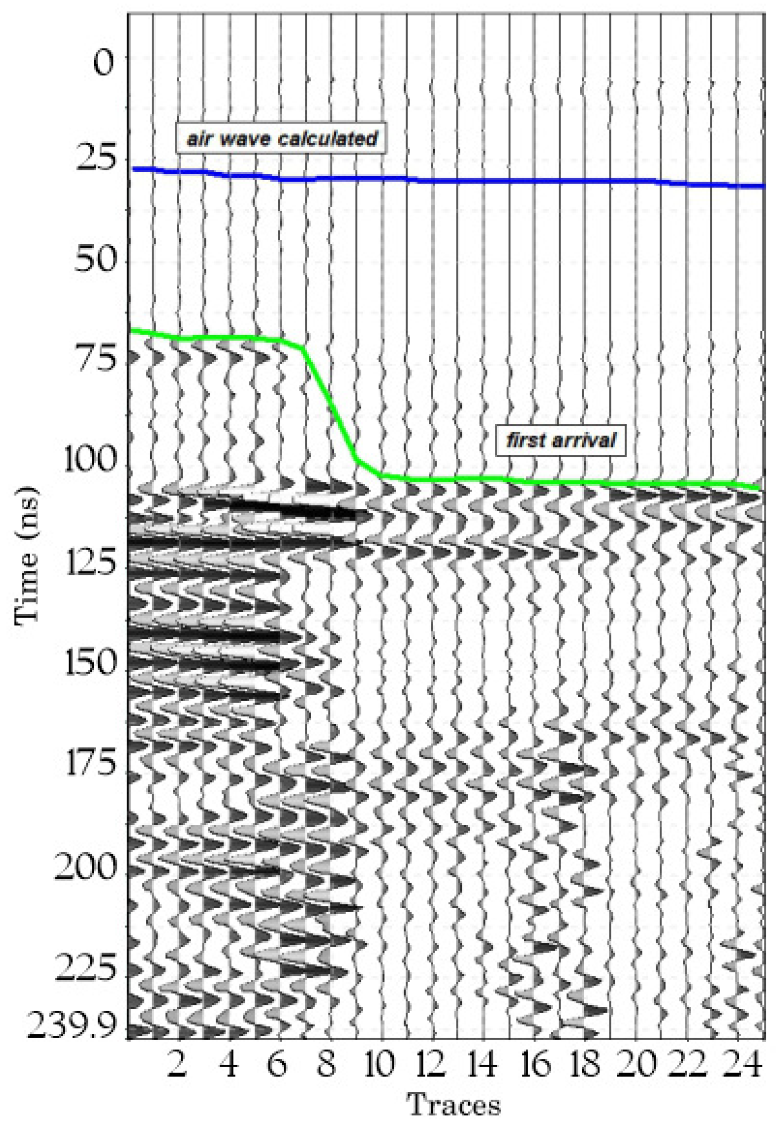
The first arrival in these B-scans can be identified as the first significant change in amplitude. The period of small or no response in each trace is the time elapsed by the pulse between the transmitting and receiving antenna on the other side of the exposed face.
2.4. Acquisizione B-Scan gpr
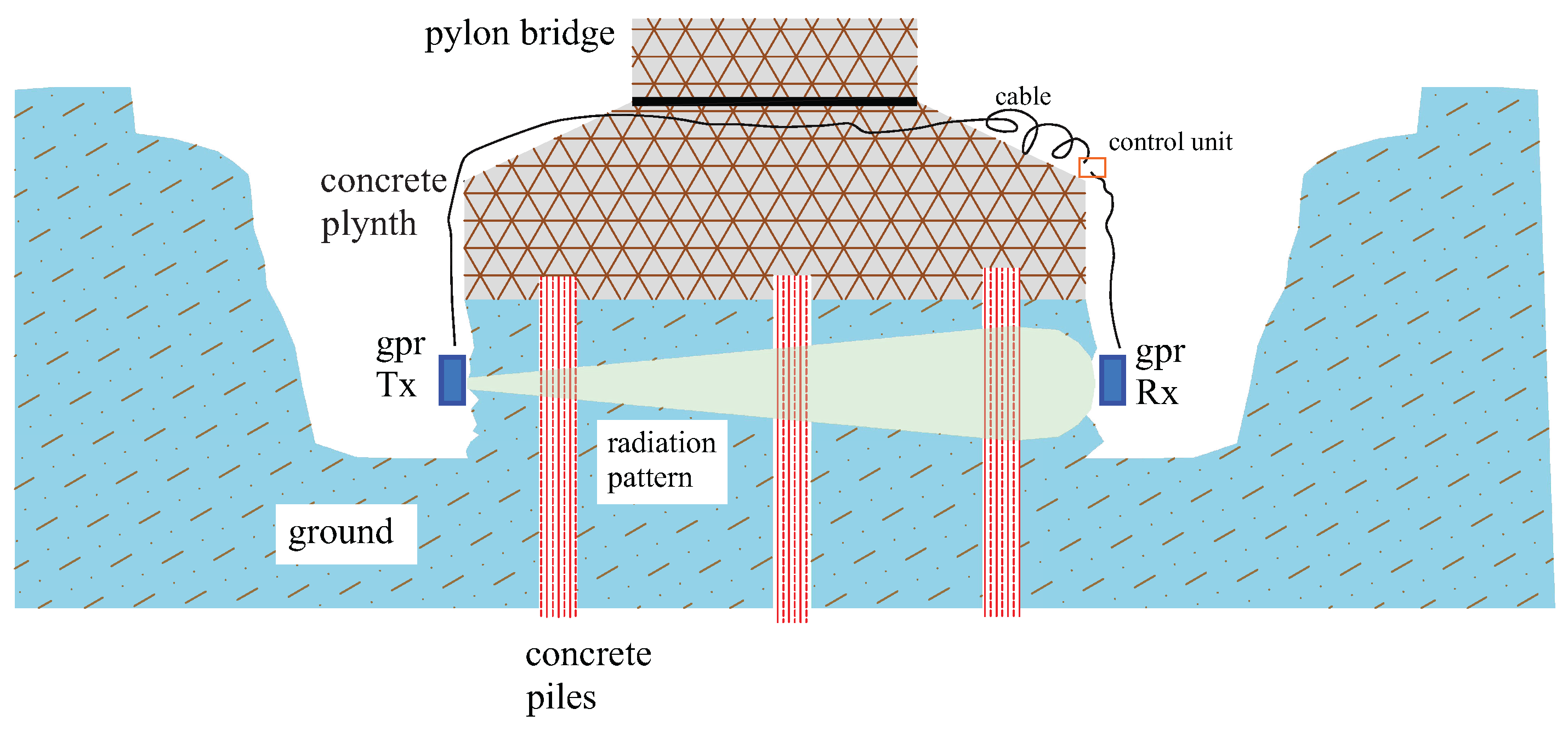
Four B-scan profiles were acquired in single-fold mode. The 200-Mhz Tx transmitting antenna is placed on one side of the trench, at the base of the excavation, while the 300-Mhz receiving antenna is placed on the opposite side, also at the base in the same origin point. In this way, the radar energy is directed along a straight line from the transmitting antenna to the receiving antenna placed at a known distance. The elongated illumination cone of the antenna can so transmit electromagnetic energy into the adjacent layers regardless of the orientation of the antennas and investing all objects and the ground along the radiation pattern.
Figure 6.
Schematic of B-scan acquisitions with separate Tx and Rx antennas placed on opposite sides of each side of the bottom trench, the long cable connecting to the control unit.
Figure 6.
Schematic of B-scan acquisitions with separate Tx and Rx antennas placed on opposite sides of each side of the bottom trench, the long cable connecting to the control unit.
The acquisition parameters are grouped here in the first 4 columns; in the remaining ones are the values estimated using Mhz, , mS/m.

Table 1.
Acquisition parameters in bistatic configuration.
| Time Window | Stack n. Traces | Sample n. | Realtime Filter | Wavelenght Medium | ; | Subfoot (m) | Mhz | Loss Tangent | Q-Estimation |
|---|---|---|---|---|---|---|---|---|---|
| 200 ns | 4 | 512 | no | 0.27 m | 0.14; 0.07 | 2.2; 1.11 | 1280 | 2.24 | 30 |
1 First numer is semimajor axes and second is semiminor axis.
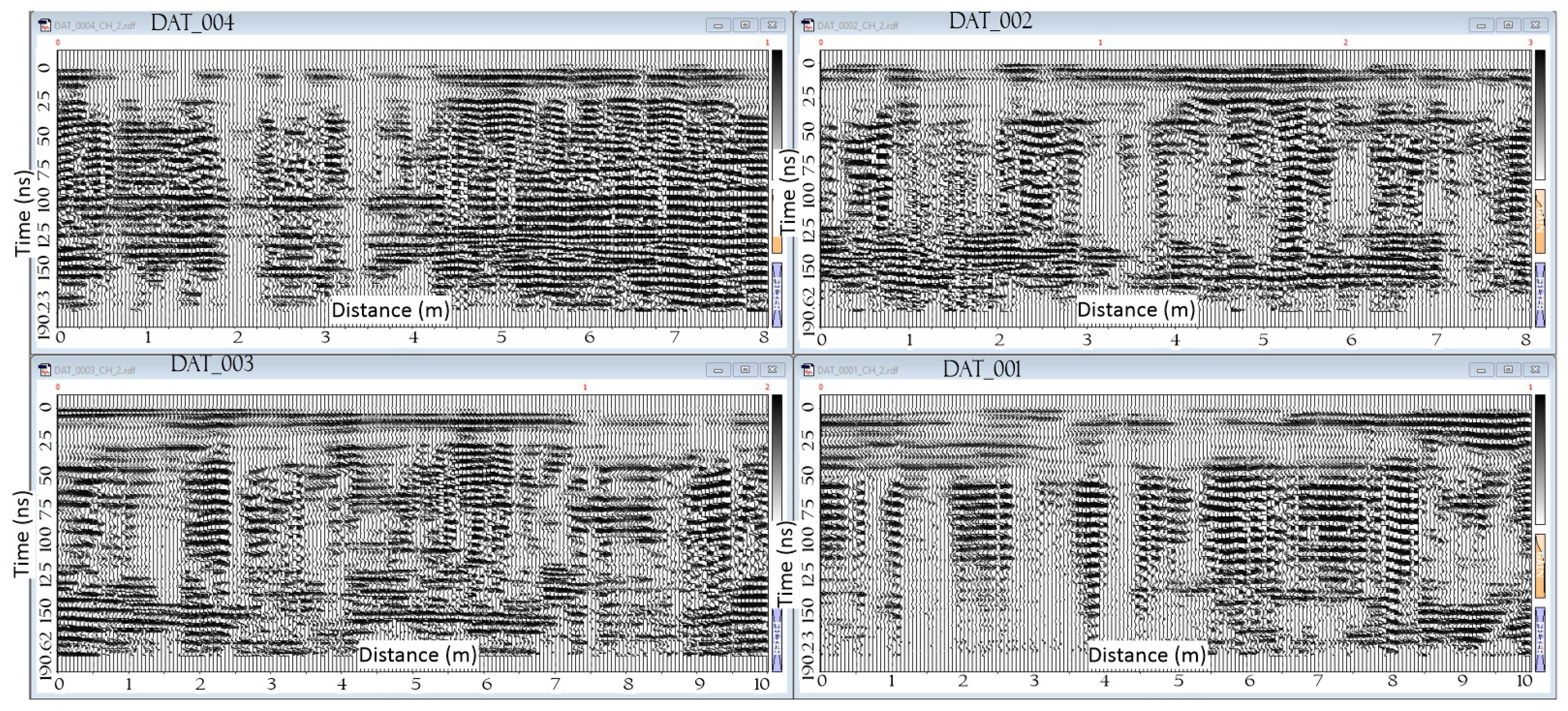
The acquired radargrams are here grouped in the form of horizontally compressed wiggle plots. The wiggle plot is a collection of single traces with no color intensity and the visual aspect focuses on the shape and pattern of the data, to the deviation in positive and negative values from a baseline such as the reference polarity. The polarities, positive and negative, of the reflection provide much information about the type of material from where it comes. A change in polarity can help in the interpretation of data by indicating a transition from a metallic to a plastic object, for example.
Figure 7.
Radargrams from DAT_001, bottom right to DAT_004 top left. The wiggle plot shows the combination of series of A-scan.
Figure 7.
Radargrams from DAT_001, bottom right to DAT_004 top left. The wiggle plot shows the combination of series of A-scan.
2.5. Processing gpr Data
In order to generate GPR signals with adequate signal to noise ratio (SNR) to extract meaningful information from the radargram, GPR data processing is implemented. The following data processing helps to reduce clutter or eliminated unwanted noise in the data set:
- time-zero correction to ensures that all reflections are correctly aligned by setting the airwave and direct wave of the trace at the first break point (or the first negative lobe) to a particular time-zero position
- background signal removal that is present at the beginning of a radar signal known as the direct wave dovuto all’accoppiamento dell’antenna con la faccia verticale della trincea. This part of the signal is considered as unwanted noise or clutter
- exponential gain to equalize the amplitude of the emitted wave, which suffers a significant attenuation along the medium
-
Ormsby bandpass filter along a trace for low-frequency interference and signal’s high-frequency components suppression. The algorithm used comprises three steps:application of direct FFT (fast Fourier transform) for transition from the time domain into the frequency domain of low-frequency and high-frequency trace spectrum components suppression and application of reverse FFT for transition from the frequency domain into the time domain
- time-depth conversion should be used for restructuring the initial time profile into a depth profile in compliance with the velocity areas.
2.6. Back Scattering Field Analysis (BSEF)
When terrain features change smoothly, without jumps, or caused by to the diffuse nature of adjacent layers, it is difficult to distinguish from visual analysis of the data, variations or radar reflections [24] and the only solution is to manually determine, as known in geophysical techniques, the velocity characteristics of discontinuities in radargrams based on diffracted waves, which were formed as a result of reflections from point objects in the subsurface and combine areas with similar velocity values in layers. When an electromagnetic wave impinges on the interface between two medias with different dielectric properties, a part of its energy is backscattered [25,26] and the remainder is transmitted into the lower medium. The directions of the incident, reflected and transmitted wave are related to each other by Snell’s law. The radiation pattern in the real case of inhomogeneous media becomes increasingly diffuse, and backscattering tends to increase. Part of the transmitted energy is scattered at the inhomogeneities and can pass through the upper medium to the surface [24]. Scattering, which is called volume scattering, is weaker than a surface scattering because it causes a redistribution of energy in the transmitted wave in multiple directions, resulting in energy loss. The total loss that an electromagnetic wave experiences in a physical medium is the sum of the loss due to diffusion and the loss due to conduction [27]. The radar backscatter of an object, as mentioned by Toropainen [28], is measured in decibel (dB) using Equation (8):
where the first term represents the backscatter of the incident wave, the second term represents the forward scattered wave, the third term represents the reduced incident wave’s backscatter, represents the voltage reflectance coefficient at lower surface, represents cross-section of the material and d is the distance travel by the signal. With these reflection patterns, that recorded in the radargram, the material properties of the subsurface heterogeneities can be extracted directly through close inspection. From this premise, it seems natural to use the backscatter field [29] of electromagnetic waves to determine the electrophysical structure of the propagating medium [30]. One of the advantages of BSEF analysis is the ability to study the subsurface, whose electrophysical characteristics change vertically uniformly, without sudden jumps and cannot form reflections. In such soils, often, only high-frequency noise and various types of interference are present on the GPR profile, provided that the medium does not contain local objects. Local subsurface objects are defined as those whose linear dimensions are comparable to the wavelength of the GPR antenna pulse and whose electrophysical characteristics differ from those of their encompassing medium [26]. They become a source of diffracted waves, whose kinematic and dynamic characteristics contain information about the properties of the subsurface. With this analysis, the attribute sections are obtained [29] to study the subsurface even in the absence of reflections from the layer boundaries. The backscattered wavefield attributes of the GPR profile are quantitative characteristics of a recording. Based on the wavefield attributes, subsurface attributes such as permittivity, humidity, electrical resistivity, conductivity, amplitude, frequency, phase, attenuation etc. are calculated. With this our processing, the attribute section Weighted average frequency was studied, which is the weighted average frequency [26] of the spectrum of the reflected signal, calculated by the formula,
where is the spectral amplitude at the frequency measured in MHz.
3. Results
Survey results are represented, in order, according to velocity tests and bistatic scans in common-offset single fold.
3.1. Velocity Test Results
The results of the two CMP velocity tests, shown in the table below, demonstrate that the velocity of the EM wave undergoes a clear variation propagating through the plinth and then into the encompassing soil. The velocity of the soil outside the plinth also shows values consistent with the lithologies present. In addition, the clay component of the soils and their moisture did not result in a lowering in propagation velocity.
Table 2.
Velocity and dielectric permittivity of the tested layers.
| ID | Thickness (m) | Velocity (cm/ns) | Permittivity | Error [RMS] | Layer |
|---|---|---|---|---|---|
| CMP1 on trench | 0.959 | 9.785 | 9.400 | 0.109 | 1 |
| 1.684 | 8.036 | 13.938 | 0.016 | 2 | |
| CMP2 on plynth | 1.102 | 11.743 | 6.527 | 0.319 | 1 |
| 2.469 | 8.148 | 13.558 | 0.001 | 2 |
In the transillumination test, first arrivals, distances, and depths of travel of antennas were measured:
Table 3.
Zero -offset transillumination test results.
| Trace | Depth (cm) | Distance (cm) | Time (ns) | Velocity (cm/ns) | |
| 1 | 0 | 800 | 65.27 | 12.26 | 5.98 |
| 2 | 10 | 800 | 66.86 | 11.97 | 6.28 |
| 3 | 20 | 800 | 67.44 | 11.86 | 6.39 |
| 4 | 30 | 800 | 66.86 | 11.97 | 6.28 |
| 5 | 40 | 800 | 66.86 | 11.97 | 6.28 |
| 6 | 50 | 800 | 66.86 | 11.97 | 6.28 |
| 7 | 60 | 800 | 67.44 | 11.86 | 6.39 |
| 8 | 70 | 800 | 69.2 | 11.56 | 6.73 |
| 9 | 80 | 800 | 85.04 | 9.41 | 10.15 |
| 10 | 90 | 800 | 96.18 | 8.32 | 12.99 |
| 11 | 100 | 800 | 97.94 | 8.17 | 13.47 |
| 12 | 110 | 800 | 97.94 | 8.17 | 13.47 |
| 13 | 120 | 800 | 98.52 | 8.12 | 13.63 |
| 14 | 130 | 800 | 99.11 | 8.07 | 13.79 |
| 15 | 140 | 800 | 99.7 | 8.02 | 13.96 |
| 16 | 150 | 800 | 100.87 | 7.93 | 14.29 |
| 17 | 160 | 800 | 105.87 | 7.56 | 15.74 |
| 18 | 170 | 800 | 104.46 | 7.66 | 15.32 |
| 19 | 180 | 800 | 105.35 | 7.59 | 15.59 |
| 20 | 190 | 800 | 104.9 | 7.63 | 15.45 |
| 21 | 200 | 800 | 105.66 | 7.57 | 15.68 |
| 22 | 210 | 800 | 105.75 | 7.56 | 15.71 |
| 23 | 220 | 800 | 106.57 | 7.51 | 15.95 |
| 24 | 230 | 800 | 106.92 | 7.48 | 16.05 |
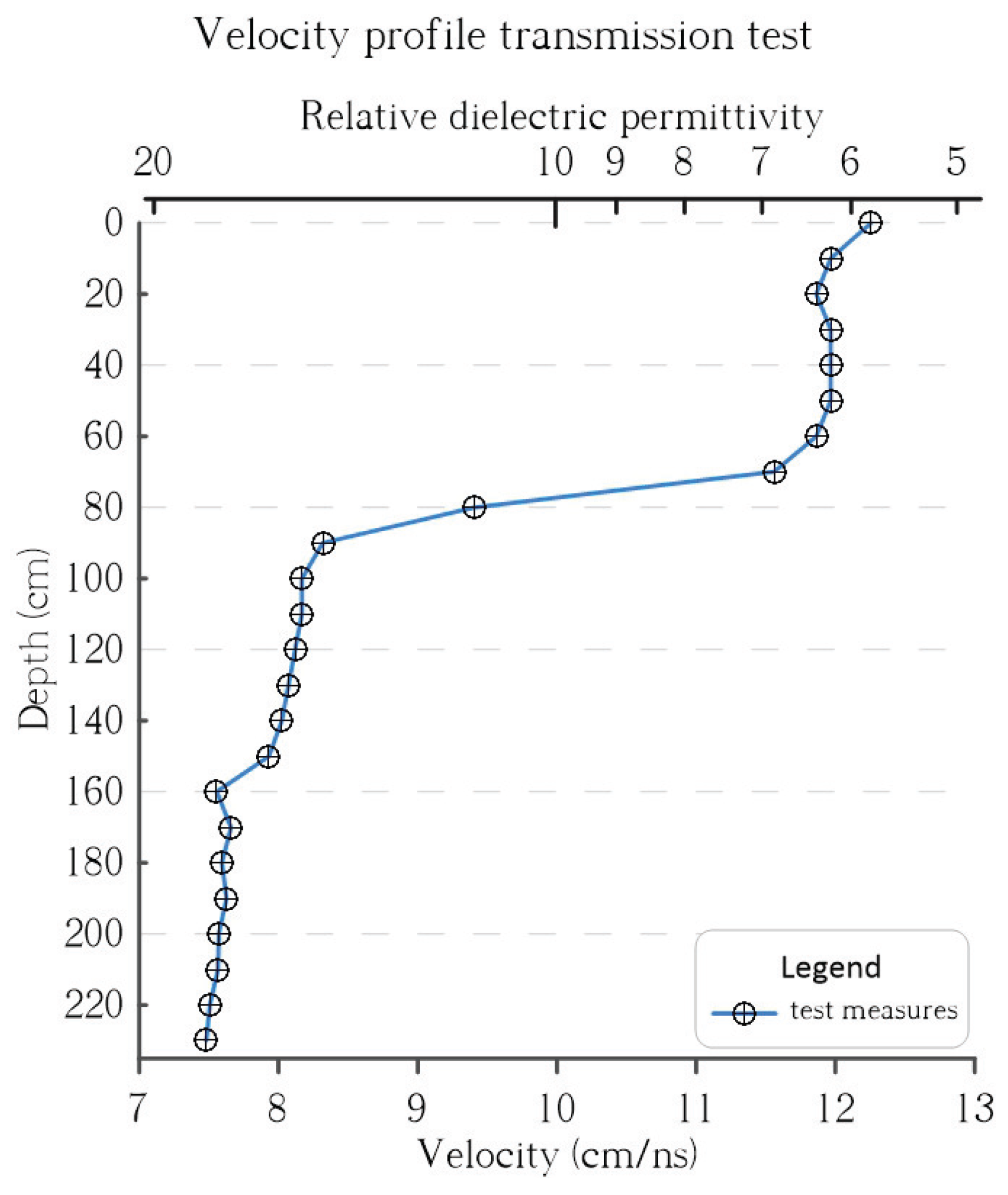
Knowing the horizontal separation between antennas and the travel time of the radar energy at each point, the velocity (Table 3) and relative dielectric permittivity can be calculated. The velocity measurements, at each point, thus represented as a function of antenna depth, show the trend in the tested material, any gradient or whether there are jumps. In this case, a dip between 70 and 100 cm depth is noted (measurements started from above), which corresponds to the interface between the plinth and the underlying soil on which it rests.
Figure 8.
Graph of velocity and dielectric permittivity (in logarithmic scale) as a function of measurement depth.
Figure 8.
Graph of velocity and dielectric permittivity (in logarithmic scale) as a function of measurement depth.
The conducted velocity tests were used to explore the dielectric permittivity field across the media to be investigated and use them for BSEF analysis. During the GPR investigation of the soil under the foundation, 4 GPR profiles were recorded. Analysis of each of these B-scan GPR profiles produced no results and no visual evidence of amplitude anomalies that could be directly interpreted from radargrams and correlated with the target under investigation. It became necessary to combine these 4 profiles into a single set. In general, this can be done easily if the GPR profiles have the GPR pulses propagating in one direction. In this particular case, however, the GPR antenna radiation propagates in the same plane, but in different directions as the antennas move along a perimeter. With the help of BSEF analysis and the contribution of R. Denisov, the sections of the 4 radargrams of the attribute “Weighted Average Frequency” were first combined to obtain a perimeter tomography.
Figure 9.
Result of BSEF analysis and combined section of the attribute Weighted average frequency (in Mhz), the arrows highlight the 4 anomalies.
Figure 9.
Result of BSEF analysis and combined section of the attribute Weighted average frequency (in Mhz), the arrows highlight the 4 anomalies.
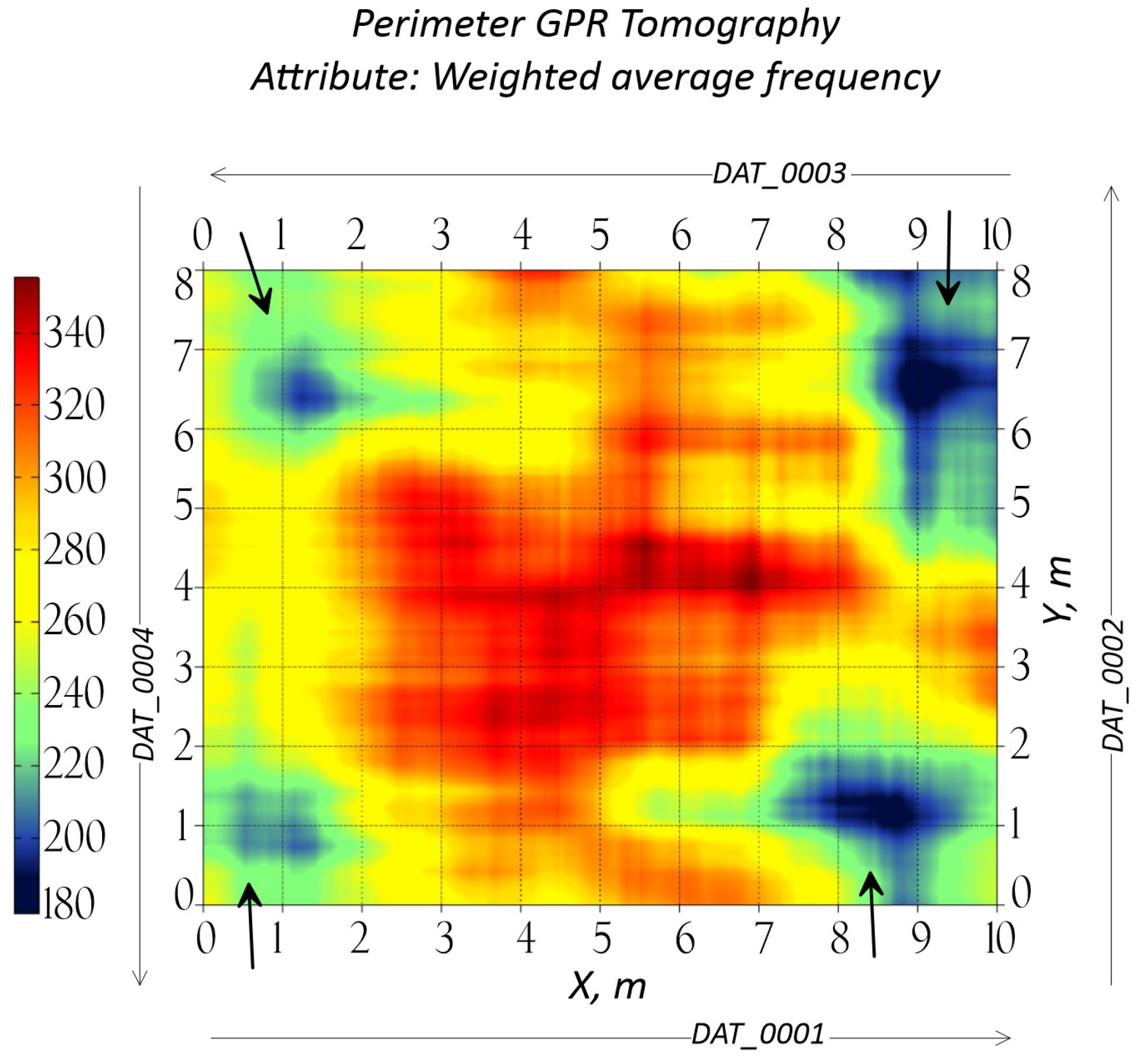
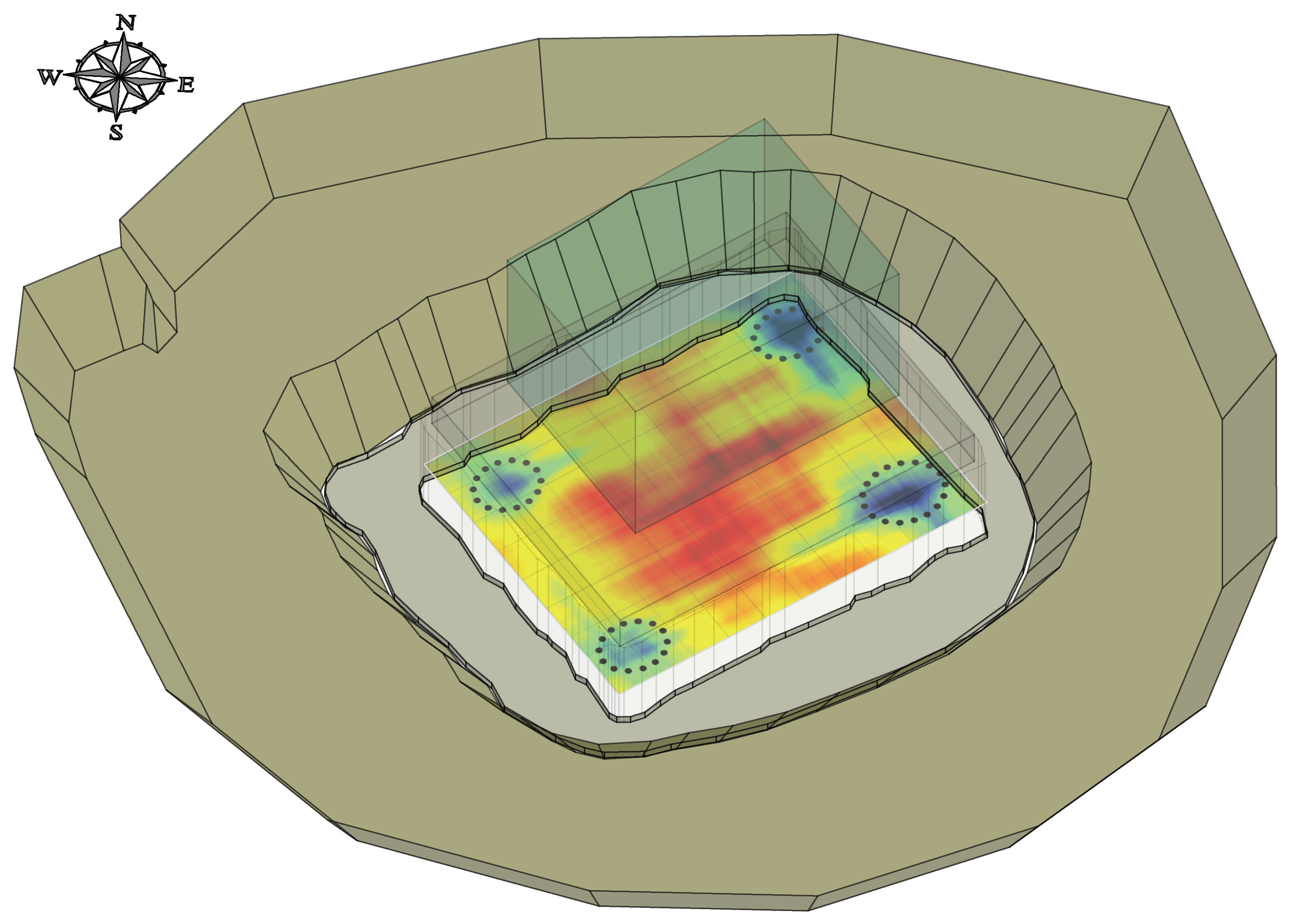
Here, 4 anomalies were identified, comparable in size to drilled piles with a diameter of 0.8 m. These anomalies are located at the corners of the foundation a little less than 1 m inward. In the following 3D image, the perimeter and horizontal tomographic section is placed in the ground and makes the pile anomalies visible (circled with black dotted lines).
Figure 10.
Overlay of the perimeter tomography to the 3D model of the structure investigated below the plinth. The anomalies of the poles have been circumscribed here.
Figure 10.
Overlay of the perimeter tomography to the 3D model of the structure investigated below the plinth. The anomalies of the poles have been circumscribed here.
4. Discussion
We conducted a study on the search for bored piles below a large and deep foundation using medium-low frequency GPR methods. The possibility of exploring with GPR the base of the plinths, thick and placed 4 m from the ground level, is intricate given the unfavorable geometry of the target. Although the depths to be reached fall within the investigation depth achievable with the GPR, any scans made from the ground level and therefore a few meters away from the pile head, would not produce easily interpretable results. In fact, if you move away with the radar, from the cutting plane of the piles, the angle between the target and the radiation lobe of the GPR, with respect to the vertical, becomes increasingly smaller. Conversely, the same scans performed below the plinth on which they rest produced the anomalies, but combining the sections in the form of "perimeter tomography". In fact, the scans are performed on the same plane, but in different directions. The results show a favorable accuracy that emerged with a robust analysis of the data with respect to the chosen detection geometry. Further studies will expand this work and will be aimed at investigating the variation of the minimum and maximum angle between the target and the radiation lobe of the antennas, with respect to which the presence of the poles could still be probed, moving the antennas along the vertical axis.
Funding
This research received no external funding.
Institutional Review Board Statement
Not applicable
Informed Consent Statement
Not applicable
Data Availability Statement
No data is associated with this research
Acknowledgments
I thank Roman R. Denisov for his technical contribution, his computer support and advices and checks on data processing. I thank Dr. geol. Paolo Spallacci for the opportunity provided to perform the georadar surveys.
Conflicts of Interest
The authors declare no conflicts of interest.
Abbreviations
The following abbreviations are used in this manuscript:
| MDPI | Multidisciplinary Digital Publishing Institute |
| DOAJ | Directory of open access journals |
| GPR | Ground Penetrating Raadar |
| CMP | Common Mid Point |
| RDP | Relative Pemittivity Dielectric |
| EM | Electromagnetic |
| Tx | Transmitter |
| Rx | Receiver |
| SNR | Signal to Noise Ratio |
| BSEF | Back Scattering Electromagnetic Field |
References
- Paoletti V.; D’Antonio D.; De Natale G.; Troise C.; Nappi R. Large-Depth Ground-Penetrating Radar for Investigating Active Faults: The Case of the 2017 Casamicciola Fault System, Ischia Island (Italy). Applied Sciences 2024. [CrossRef]
- Nappi R.; Paoletti V.; D’Antonio D.; Soldovieri F.; Capozzoli L.; Ludeno G.; Porfido S.; Michetti A. M. Joint Interpretation of Geophysical Results and Geological Observations for Detecting Buried Active Faults: The Case of the “Il Lago” Plain (Pettoranello Del Molise, Italy). Remote Sensing 2021, p. 8. [CrossRef]
- Alani A. M.; Morteza A.; Gokhan K. Applications of Ground Penetrating Radar (GPR) in Bridge Deck Monitoring and Assessment. Journal of Applied Geophysics 2013, pp. 45–54.
- Soldovieri F.; Persico F.; Utsi E.; Utsi V. The Application of Inverse Scattering Techniques with Ground Penetrating Radar to the Problem of Rebar Location in Concrete. NDT & E International 2006, pp. 602–607.
- D’Antonio D.; Di Stefano S.; Faustoferri A.; De Leo A. Opi (AQ) Ponte Romano Sul Sangro. Quaderni di Archeologia d’Abruzzo 2014, 5, 128–134.
- Lai W. L.; Kou S. C.; Tsang W. F. Characterization of Concrete Properties from Dielectric Properties Using Ground Penetrating Radar. Cement and Concrete Research 2009, pp. 687–695.
- Tosti F.; Slob E. Determination, by Using GPR of the Volumetric Water Content in Structures, Substructures, Foundations and Soil, Civil Engineering Applications of Ground Penetrating Radar. Springer Transaction in Civil and Environmental Engineering 2015.
- Zhou D.; Zhu H. Application of Ground Penetrating Radar in Detecting Deeply Embedded Reinforcing Bars in Pile Foundation. Hindawi Advances in Civil Engineering 2021, p. 13.
- Bradford J. H. Frequency Dependent Attenuation of GPR Data as a Tool for Material Property Characterization: A Review and New Developments. Proceedings of 6th International Workshop on Advanced GPR 2011, pp. 1–4.
- Grandjean G.; Gourry J. C.; Bitri A. Evaluation of GPR Technique for Civil-Engineering Applications: Study on a Test Site. Applied Geophysics 2000, pp. 141–156. [CrossRef]
- Annan A. P. Ground Penetrating Radar Principles, Procedures and Applications, s. & s. ed.; Vol. 278, Sensors & Software Inc.: New York, 2003.
- Davis J. L.; Annan A. P. Ground Penetrating Radar for High-Resolution Mapping of Soil and Rock Stratigraphy. Geophysics 1989, pp. 531–551.
- Annan A. P.; Cosway S. W. Symposium on the Application of Geophysics to Engineering and Environmental Problems. Ground Penetrating Radar Survey Design 1992.
- Daniels D. J. Ground Penetration Radar, 2nd ed.; Number 15 in IEE Radar, Sonar and Navigation, Institut of Engineering Technology: London, 2004.
- Burger H.R. Exploration Geophysics of the Shallow Subsurface, englewood cliffs ed.; Print Hall: New Jersey, 1992.
- Conyers L. B. Ground-Penetrating Radar for Archaeology; AltaMira Press: Walnut Creek, 2004.
- Lavoue F. 2D Full Waveform Inversion of Ground Penetrating Radar Data: Towards Multiparameter Imaging from Surface Data. Sigillum Universitatis Gratianopolitane 2014.
- Klysz G.; Balayssac J. P. Determination of Volumetric Water Content of Concrete Using Ground-Penetrating Radar. Cement and Concrete Research 2007. [CrossRef]
- Moysey S.; Knight R. J. Modeling the field-scale relationship between dielectric constant and water content in heterogeneous systems. Water Resources Research 2004, p. 40.
- Jonscher A. K. Modeling the field-scale relationship between dielectric constant and water content in heterogeneous systems. Journal of Physics D: Applied Physics 1999, pp. 57–70.
- Olhoeft, G. R. Maximizing the Information Return from Ground Penetrating Radar. Journal of Applied Geophysics 2000, pp. 175–187. [CrossRef]
- Giannopoulos A. GprMax2D V 1.5 User’s Manual, 2002.
- Persico R. Introduction to Ground Penetrating Radar: Inverse Scattering and Data Processing; Wiley-IEEE Press, 2014.
- Radzevicius S.; Daniels J. J. Ground Penetrating Radar Polarization and Scattering from Cylinders. Journal of Applied Geophysics 2000, pp. 111–125. [CrossRef]
- Langley K. A.; Hamrain S. E. Use of C-band Ground Penetrating Radar to Determine Backscatter Sources within Glaciers. IEEE Transactions on Geoscience and Remote Sensing 2005.
- Denisov R. R. Processing of georadary data in automatic mode. Scientific and Technical Journal Geophysics 2010, pp. 76–80.
- Ulaby F. T.; Moore R. K.; Fung A. K. Microwave Remote Sensing Active And Passive Volume Ii Radar Remote Sensing And Surface Scattering And Emission Theory; Vol. II, Radar Remote Sensing And Surface Scattering And Emission Theory, Addison-Wesley Publishing Company, 1982.
- Toropainen A.P. Measurement of the Properties of Granular Materials by Microwave Backscattering. Journal of Microwave Power and Electromagnetic Energy 1995, pp. 240–245. [CrossRef]
- González R. C.; Woods E. C.; Eddins S. L. Digital Image Processing Using MATLAB; Pearson Prentice Hall, 2003.
- Ivan Levyant V. B.; Petrov Pankratov S. A. Seismic Exploration Technologies. Research of the characteristics of longitudinal and exchange waves of retroactive response scattering from the zones of the cracked collector 2009, pp. 3–11.
Disclaimer/Publisher’s Note: The statements, opinions and data contained in all publications are solely those of the individual author(s) and contributor(s) and not of MDPI and/or the editor(s). MDPI and/or the editor(s) disclaim responsibility for any injury to people or property resulting from any ideas, methods, instructions or products referred to in the content. |
© 2025 by the authors. Licensee MDPI, Basel, Switzerland. This article is an open access article distributed under the terms and conditions of the Creative Commons Attribution (CC BY) license (http://creativecommons.org/licenses/by/4.0/).
Copyright: This open access article is published under a Creative Commons CC BY 4.0 license, which permit the free download, distribution, and reuse, provided that the author and preprint are cited in any reuse.


