
Submitted:
30 May 2025
Posted:
06 June 2025
You are already at the latest version
Abstract
This study evaluates the performance of count regression models in the presence of zero inflation, outliers, and overdispersion using both simulated and real-world maternal mortality dataset. Traditional Poisson and Negative Binomial regression models often struggle to account for the complexities introduced by excess zeros and outliers. To address these limitations, this study compares the performance of robust zero-inflated (RZI) and robust hurdle (RH) models against conventional models using the Akaike Information Criterion (AIC), Bayesian Information Criterion (BIC), and the Vuong test to determine the best-fitting model. Results indicate that the robust zero-inflated Poisson (RZIP) model performs best overall. The simulation study considers various scenarios, including different levels of zero inflation (50%, 70%, and 80%), outlier proportions (0%, 5%, 10%, and 10 15%), dispersion values (1, 3, and 5), and sample sizes (50, 200, and 500). Based on AIC comparisons, the robust hurdle Poisson (RZIP) and robust hurdle Poisson (RHP) models demonstrate superior performance when outliers are absent or limited to 5%, particularly when dispersion is low (1 or 3). However, as outlier levels and dispersion increase, the robust zero-inflated negative binomial (RZINB) and robust hurdle negative binomial (RHNB) models outperform robust zero-inflated Poisson (RZIP) and robust hurdle Poisson (RHP) across all levels of zero inflation and sample sizes considered in the study.
Keywords:
robust regression
; count data
; outliers
; overdispersion
; zero inflation
; maternal mortality
1. Introduction
Excess zeros are common in numerous fields, including healthcare, agriculture, ecology, and manufacturing industries [1,2]. A Zero-Inflated (ZI) model [3] argues that zero counts arise from a combination of two distributions: One distribution generates structural zeros, representing subjects who are not at all at risk of experiencing the event (and thus consistently produce zero counts). For instance, when quantifying specific high-risk behaviors, certain individuals may record a score of zero due to their lack of susceptibility to such health-risk behaviors [4]. The second distribution generates sampling zeros, representing individuals who are at risk but did not experience or report the event during the study period.
The justification for categorizing zeros into two categories is that a high proportion of zeros frequently results from the presence of a subgroup of patients who are not at risk for certain outcomes during the study period [3]. The probability of belonging to the zero inflation component is assessed using a zero-inflation probability model, while a standard count distribution, such as Poisson or Negative Binomial, represents the counts in the count component [5]. Conversely, a hurdle model [6] claims that all zero observations originate from a singular structural source, comprising a binary component to determine whether the response variable is zero or positive, alongside a truncated model, such as a truncated Poisson or truncated Negative Binomial distribution, for the positive data. Excess zeros indicate more zeros than the distribution we are modeling would expect. Zero-inflated and hurdle models have been used extensively in various research domains to model such data [2,7]. The traditional models, such as the standard Poisson and Negative Binomial models, often fail to address the complexity of outliers, overdispersion, and excess zeros simultaneously. The understanding and useful comparison of the robust zero-inflated (RZI) and robust hurdle (RH) models remain largely unexplored, despite substantial advances in statistical modeling methods for count data [1,2]. Although both models address the frequent excess zeros seen in the count data, their fundamental tenets and estimating strategies are different.
Maternal mortality data often exhibit zero inflation, characterized by an excess of zero counts or units reporting no maternal deaths, compared to what standard count models such as Poisson or Negative Binomial would predict. [8,9]. Identifying factors that contribute to maternal mortality and formulating effective interventions is essential to minimize the increase in maternal mortality. In this context, there is a need to employ statistical models that can adequately handle the excessive zeros, overdispersion, and potential outliers that are often observed in maternal mortality [10]. Previous studies that have looked at factors affecting maternal death have used different analysis strategies, with some ignoring the underlying zero inflation [11,12].
Comparison of zero-inflated models with hurdle models is the main emphasis of the currently available literature on count data analysis with excessive zeros and outliers [2,10,13]. However, the robustness to outliers that these comparisons frequently neglect can have significant effects on the accuracy and reliability of the models’ results. Robust zero-inflated models and robust hurdle models have been proposed to handle outliers in addition to zero inflation. There is a lack of comprehensive studies that directly examine the performance of robust hurdle and zero-inflated models in the presence of outliers. In addition, there has been little research on the application of these models to maternal mortality data [1,2,12], an important public health indicator. Using simulated data and data on maternal mortality, this study attempts to close these gaps by comparing the robust zero-inflated and hurdle models in the presence of outliers. Through this investigation, the study hopes to shed light on how well these models handle excessive zeros and outliers in count data, with an emphasis on enhancing modeling accuracy and forecasting rates of maternal death.
2. Methods
2.1. Overview of Count Data Models
2.1.1. Robust Zero-Inflated Models
Although ZIP and ZINB models handle excess zeros, they can be sensitive to outliers. The RZIP and RZINB models improve the standard ZI models by incorporating robust estimation techniques. The robust zero-inflated models (RZIP and RZINB), first proposed by [5] and later refined by [14], integrate Huber’s M-estimation into standard ZIP/ZINB structures. The robust approach uses the Huber -function [15], to downweight extreme values during parameter estimation. In the RZI models, the parameters are estimated using a robust Expectation-Maximization (EM) algorithm by [5]. The M-step replaces traditional estimators with robust ones, using the function to assign lower weights to observations in the tails of the distribution:
where and are the c and (1-c) quintiles of the Poisson component [15]. The robustified equations in the M-step for the parameters of the RZI models and are given by:
For the zero-inflation component:
For the count component:
where and are weights designed to mitigate the influence of outliers, defined as a similar definition applies to and represents an expected value for -Huber function. These robust adjustments help reduce the influence of outliers, making the RZI models more reliable in practice [5,14].
2.1.2. Robust Hurdle Models
The robust hurdle models used in this study build upon the methodology developed by [16], who proposed a robust version of the hurdle models that are based on standard hurdle models by incorporating bounded-influence estimation through the Huber -function to mitigate the influence of outliers [17]. For the binary hurdle component, we replace the standard logistic regression with a robust logistic regression using the -Huber function [15]. This ensures that outliers in the binary classification of zeros and non-zeros have less influence. The robust binary hurdle equation is given by:
where is an indicator variable for whether , and are robust weights to downweight outliers [18]. For the positive count component, the traditional count regressions are replaced with a robust count regression using the -Huber function [5,10]:
Here, is the Huber function that reduces the impact of large residuals (outliers), and weights are used further to control the influence of outliers. By robustifying both the binary hurdle and positive count components, the RH models are more resistant to data irregularities like outliers [10]. This robust approach ensures that extreme values and outliers do not overly affect the estimation of parameters, making the robust hurdle models more reliable in real-world data applications.
2.2. Simulation Study
Three different sample size scenarios (50, 200, and 500) were taken into account for the simulated dataset under the Negative Binomial distributions. For the count data produced using the NB distribution, various dispersion levels (1, 3, and 5) were taken into account for each sample size, along with structural zeros (0.5, 0.7, and 0.8) and outliers (0.0, 0.05, 0.10, and 0.15). A summary of the simulation scenarios considered in the study is shown below in Table 1. This produced 3 × 3 × 3 × 4 = 108 distinct simulation scenarios in all. Each scenario was run 1000 times to reduce the influence of simulation error, and the outcomes were averaged over the 1000 runs.
2.3. Model Comparison
To assess the performance of the six different models under different simulation scenarios, the study adopted the widely used model selection criteria: Akaike’s information criteria (AIC) developed by [19]. AIC has been presented as a model selection criterion for comparing non-nested models based on maximum likelihood, utilizing the fitted log-likelihood function to identify the optimal model. The AIC evaluates the relative quality of a statistical model by rewarding goodness of fit while imposing a penalty that increases with the number of estimated parameters. As the log-likelihood is anticipated to rise with the addition of parameters to a model, the AIC criterion imposes a penalty on models with a greater number of parameters (q). The penalty function may also depend on n, the number of observations. This penalty prevents overfitting. Consequently, the AIC is defined as
where L is the maximal likelihood function value for the estimated model, q is the number of degrees of freedom, and 2 is a tuning parameter to balance the information in the model with the residuals, according to the number of degrees of freedom. It is desirable to choose a model with the lowest AIC.
The Bayesian Information Criterion (BIC) is defined as:
where L is the likelihood of the model, k is the number of parameters, and n is the sample size. When fitting models, it is possible to increase the likelihood by adding parameters, but doing so may result in overfitting. The BIC addresses this issue by introducing a penalty term for the number of parameters in the model. The penalty term in BIC is larger than the penalty term in AIC. The AIC was averaged in each of the simulation scenarios over 1000 repetitions.
For comparing non-nested models with different probability mass functions and , the Vuong test [20] is employed. The test statistic V is calculated as , where m is the mean of , is the standard deviation of , and n is the sample size. Here, . The Vuong test statistic follows a standard normal distribution. For example, at a significance level of 0.05, the first model is considered "closer" to the actual model if ; conversely, the second model is deemed "closer" if . If , neither model shows superiority over the other, suggesting no significant difference in model fit. In cases where models have unequal numbers of parameters, is adjusted to , where and are the number of parameters in models 1 and 2, respectively. This adjustment accounts for the difference in parameter complexity between the models, ensuring a fair comparison in model selection based on their respective fit to the data.
3. Results
3.1. Simulation Study Findings
3.1.1. Initial Assessment of the Simulation Data
The NB model in Table A1 consistently achieves the lowest AIC across all sample sizes for the initial assessment of the simulation, where the parameters are set to zero, such as the inflation and outliers, confirming it as the best fit for data generated from an NB distribution. As expected, the NB model outperforms the Poisson model, since the data was simulated using an NB model, which is also reflected in its lower AIC value. While robust models like RZIP, RZINB, RHP, and RHNB are designed to handle complexities such as zero inflation and outliers, their AIC values remain higher in this scenario, where no excess zeros or outliers were introduced. These results emphasize the importance of selecting models aligned with the data’s underlying structure, with the NB model excelling in cases of overdispersed count data.
3.1.2. AIC Comparison Across Regression Models
In this section, we describe the analysis of data generated with the NB regression model in sixteen different simulation scenarios with varying sample sizes (50, 200, 500), different levels of outliers (0.0, 0.05, 0.10, 0.15), and magnitudes of dispersion (1, 3, 5). Table A2, Table A3, Table A4, Table A5, Table A6, Table A7, Table A8, Table A9 and Table A10 display the averaged AIC model fit statistics for Poisson, NB, RZIP, RZINB, RHP, and RHNB regression models fitted on data generated with the NB regression model with different magnitudes of dispersion, outliers, and sample sizes. The AIC values reveal that the RZINB and RHNB models generally provide the best fit for data generated from an NB model, especially under conditions of higher proportions of zeros and levels of outliers. For example, with 1 dispersion level, 0.0% outliers, and a 50% proportion of zeros, the RZIP model achieves a lower AIC than the RZINB model. As the proportion of zeros increases and outliers increase, the RZINB and RHNB models consistently show improved performance, indicating their robustness in handling zero-inflated data. Conversely, the Poisson model and NB have higher AIC values than the other models, reflecting their limitations in scenarios characterized by overdispersion and excess zeros. These results highlight the importance of selecting appropriate modeling techniques that align with the underlying data distribution and characteristics, particularly in the presence of zeros and outliers.
3.1.3. Performance under Low Outlier Levels and Increasing Dispersion
The RZIP and RHP models, when the dispersion is 5%, express superior performance in terms of model fit, particularly under conditions with no outliers (0% outlier level) or a low level of outliers (5% outlier level). This suggests that these models effectively handle zero-inflated datasets with minimal noise. Among them, the RZIP model consistently outperformed the RHP model across varying proportions of zeros (0.5, 0.7, 0.8), achieving the lowest AIC values. This highlights the robustness of RZIP in modeling highly zero-inflated data. These findings emphasize the efficacy of RZIP in accommodating zero inflation and managing datasets with either no or low extreme values. However, when the dispersion reached 3 and the sample size became 200 and above, the RZIP and RHP models demonstrated sensitivity to sample size and data characteristics as they were now outperformed by the RZINB and RHNB models. This reinforces their reliability in scenarios with increased dispersion and low levels of outliers, as evidenced by the results summarized in Table A2, Table A3, Table A4 and Table A5.
3.1.4. Performance under Moderate Outlier Levels and Increasing Dispersion
As the level of outliers in the data increases to a moderate threshold of 10% - 15%, both the RZIP and RHP models show a noticeable decline in performance when compared to more resilient models such as the RZINB and RHNB. This trend is evident even when sample size and dispersion remain constant, highlighting the limitations of the RZIP and RHP models in handling moderate to high levels of outliers. As outliers continue to increase and reach 15%, RZIP and RHP persistently lag, suggesting that these models are less effective under conditions with a substantial presence of outliers. In Table A2 through Table A10, findings consistently show that RZINB and RHNB outperform other models, especially under moderate and high outlier conditions. This higher performance is consistent across different percentages of zeros and sample sizes, making RZINB and RHNB the most reliable options for dealing with outlier-laden data.
As the dispersion parameter in the dataset increased from 3 to 5 and the proportion of outliers escalated from 0% to 5%, 10%, and 15%, notable patterns emerged in model performance. At an outlier threshold of 0%, 5%, and 10% the RZINB model demonstrated superior performance across various levels of zero-inflation (50%, 70%, and 80%) and sample sizes, archiving the lowest AIC. However, as the outlier threshold increased to 15%, the RHNB model surpassed RZINB in performance. RHNB emerged as the most reliable model under conditions of severe contamination, characterized by high proportions of outliers and substantial overdispersion. Its ability to handle excess zeros while maintaining robustness against noise induced by extreme values highlights its utility in challenging scenarios.
3.1.5. Influence of Sample Size on Model Performance
Examining the performance of RZIP, RHP, RZINB, and RHNB models across sample sizes of 50, 200, and 500 reveals key trends. Model performance varies significantly with sample size, dispersion, and outliers. RZIP and RHP perform well with smaller sample sizes (50) and dispersion of up to a maximum of 3, handling outliers up to 5% as shown in Table A5. However, as the sample size and dispersion increase or the outlier proportion exceeds 5%, these models lose accuracy. In contrast, RZINB and RHNB excel under these more challenging conditions, demonstrating superior stability and fit with larger samples, higher dispersion, and more outliers. This comparison emphasizes the importance of aligning model choice with data characteristics. RZIP and RHP are suited for simpler datasets, while RZINB and RHNB are more effective for complex datasets with greater variability and contamination.
3.2. Real Data Application
3.3. Description of the Study Sample
The empirical study sample consists of 222 patients admitted to different health organizations in Nairobi, Kenya, diagnosed with maternal health outcomes involving complications in delivery and labor. The study sample was 100% females, as expected since the focus was exclusively on maternal health. The definition of the variables in the dataset that the study uses includes maternal health outcomes and predictor variables related to delivery characteristics, maternal complications, antenatal care, and stillbirth. 3
3.3.1. Regression Diagnostics: Multicollinearity Test.
The analysis identified substantial correlations among several independent variables, indicating multicollinearity, as shown in Figure 1. This issue arises when predictor variables are highly correlated, leading to redundancy and inflated standard errors in the regression coefficients. As a result, estimates become unstable, and theoretically important variables may appear statistically insignificant, obscuring their true relationships with the outcome.
After applying the correlation-based feature selection technique, the research study reassessed the correlations among the predictors. The updated correlation matrix shown in Figure 2 and VIF values in Table 2 indicate a significant reduction in multicollinearity, confirming the effectiveness of the selection process. By removing highly correlated variables, the updated model, now free from the detrimental effects of high multicollinearity, provided more reliable and interpretable estimates. The reduction in multicollinearity is expected to improve the stability and reliability of the coefficient estimates. However, it is important to approach the interpretation of the results with caution. The relationships between predictors and the outcome variable should be evaluated within the context of the selected variables.
A list of some maternal characteristics that were considered as covariates in this study is provided in Table 3 Facilities that reported maternal fatalities and those that did not are the two categories for which the variables are presented. The percentages are calculated based on the row totals, which are the number of facilities that reported at least one occurrence from the breech birth, assisted delivery, early teen pregnancy, and late teen pregnancy categories. The largest contributing cause to maternal mortality, according to the statistics, is early teen pregnancy; 74.58% of the institutions that recorded early teen pregnancy also reported death. Other noteworthy variables include assisted delivery, late-adolescent pregnancy, and breech birth.
Table 3 displays the main clinical characteristics of the study population. The mean age for early teenage pregnancy was 10.176 and for late teenage pregnancy 18.829 .
3.4. Comparison of the Fitted Count Data Models
3.4.1. Model Evaluation
To fully assess and compare the performance of the model, the study uses the AIC and the BIC, which measure the fit of the model while penalizing complexity to avoid overfitting. Additionally, the Vuong test compares nonnested models, providing statistical evidence on whether one model significantly outperforms another. The Vuong test takes into account the model’s complexity, balancing goodness-of-fit against potential overfitting caused by increasing parameters.
3.4.2. Vuong Test
Table 4 shows the results of the Vuong test comparing different models. The significant p-values (p < 0.01 or *p < 0.001) suggest that zero-inflated and hurdle models are often better at detecting additional elements in the data, such as excess zeros, overdispersion, and outliers, compared to traditional Poisson and NB models. Although RZIP performs well in multiple comparisons and is a strong model for accurately representing the data, RHNB and RHP also demonstrate competitive performance, indicating their utility in specific contexts.
3.4.3. Model Comparison Using AIC and BIC
The comparison of all the fitted models for maternal death counts using Akaike information criteria and Bayesian information criteria. Table 5 below provides the AIC and BIC values used to choose the model that best fits the data.
The comparison of the performance of the model in Table 5 reveals that the RZIP model provided the best fit to the data, outperforming all other models based on AIC and BIC. The NB model showed considerable improvement over the standard Poisson model, indicating its ability to handle overdispersion in the data more effectively. Among the robust models, the RHP and RHNB models showed competitive performance but were still outperformed by the RZIP model. The RZINB model showed a slightly poorer fit compared to the RZIP, RHP, and RHNB models but performed better than the traditional Poisson and NB models. These findings generally emphasize the suitability of the RZIP model for this dataset, demonstrating its ability to effectively address zero inflation and outliers at approximately 5%.
In capturing the probability distribution of maternal deaths, each model shows a different performance as displayed in Figure 3, particularly for lower counts where the frequency of zeros is more prominent. The Robust Zero Inflated and Hurdle Models appear to fit the observed data more closely, as seen by their closer alignment with the black observed line for zero counts. These models, specifically designed to handle excess zeros, provide a better fit. For maternal mortality data, where zero inflation and overdispersion are likely, this suggests that robust zero-inflated and hurdle models may be more appropriate. Traditional models are outperformed by these robust count statistical models, as shown by the Voungo test and the AIC/BIC.
3.5. Robust Count Regression Estimation Results
A significant frequency of zero counts and outliers was observed in maternal mortality data. These observations were found to be beyond the anticipated range predicted by common count data distributions such as the Poisson and NB. These findings led to the theory that the data might be affected by two processes: one controlling the distribution of positive counts and another regulating the occurrence of zero occurrences. Outliers in the data suggest potential contamination with extreme values, which conventional models cannot account for. A RZIP model is more suitable for this research, as shown in Table 4 and Table 5. In the following Table 6 the study displays parameter estimates and the robust standard error of the best-performing model, which is RZIP.
Table 6 displays or represents the estimated coefficients of the RZIP model for two parts, namely the count model and the zero model. The zero model explains the excess zeros in the data, while the count model concentrates on the count (frequency) of the event, which is maternal mortality in our case. Each component describes a distinct feature of the data.
The count component of the RZIP model examines the relationship between maternal mortality and key predictors. The estimated intercept is -0.8571 (SE: 0.1514, p < 0.0001), which corresponds to an expected count of 0.4245 maternal deaths when all predictors are at their baseline levels. This significantly lower baseline suggests that, in the absence of specific risk factors, maternal mortality remains below the mean of the sample. Among the predictors, Breach Delivery has a statistically significant effect, with an estimated coefficient of 0.1159 (SE: 0.0496,p = 0.0195). This translates to a 12.3% increase in maternal mortality per unit increase in breach deliveries , reinforcing its role as a critical risk factor. Conversely, Assisted Deliveries does not exhibit a meaningful impact, with an estimated effect of -0.0038 (SE: 0.0200, p = 0.8504), corresponding to a −0.38% decrease in maternal mortality , though the effect is not statistically significant. EarlyTeenPreg, however, shows a notable association, with an estimated coefficient of 0.0568 (SE: 0.0250, p = 0.0232), indicating a 5.84% increase in maternal mortality . The statistical significance of this finding suggests that early teenage pregnancy is an important predictor of maternal mortality. LateTeenPreg, on the other hand, has an estimated effect of 0.0219 (SE: 0.0150, p = 0.1443), corresponding to a 2.21% increase in maternal mortality , but this effect is not statistically significant , indicating that it may not be a strong predictor.
The zero-inflation component of the model evaluates factors influencing the probability of an excess zero count in maternal mortality. The estimated intercept is , suggesting a significantly lower probability of zero maternal deaths when all predictors are at their baseline levels. Among predictors, BreachDelivery has an estimated effect of -0.1578 (SE: 0.4464, p = 0.7238), implying a 17.09% decrease in the odds of a zero count , although this effect is not statistically significant. Similarly, AssistedDeliveries has an estimated effect of -16.7361 (SE:15.3676, p = 0.2761) implying a -99.99% negative association with maternal mortality in the odds of a zero count , but this effect is not statistically significant. EarlyTeenPreg has an estimated
effect of 1.0192 (SE= 0.7228, p = 0.1585), suggesting that maternal mortality was a 1.77 times more likely
to occur in the EarlyTeenPreg group in maternal mortality risk . but there is a lack of
statistical significance (p > 0.05) prevents strong conclusions. In contrast, LateTeenPreg demonstrates a
significant association, with an estimated coefficient of 0.1195 (SE: 0.0464, p = 0.00100), indicating a
12.69% increase in maternal mortality risk . The statistical significance supports its role as a key predictor in the zero-inflation model, suggesting that late teenage pregnancy may influence the likelihood of maternal mortality even in cases where mortality counts are low.
3.6. The RZIP Model Validation
The overdispersion test for the Poisson model gives the following result:
with the alternative hypothesis being that the true dispersion is greater than 1. The estimated dispersion is:
Since the p-value is below the threshold of 5% level of significance, we then reject the null hypothesis; instead, we accept the alternative hypothesis, indicating that the dispersion is significantly greater than 1. That is, the variance is greater than the mean, as it was stated earlier in Table 6. This suggests that the data exhibits overdispersion, which Poisson fails to account for.
The Chi-Square test in Table 7 was used to validate the model. The test statistic is 20809.28 with 6 degrees of freedom. The p-value is 0.198, which is greater than the typical significance level of 0.05. This indicates that there is no evidence to reject the null hypothesis. Thus, the fit of the model to the data is adequate, and there is no significant lack of fit based on this test.
The likelihood ratio tests (LRT) in Table 8 were performed to compare the fit of the model with different specifications. The test between RZIP and RZINB yielded a chi-square statistic of 26.304 with a p-value of 0.06, suggesting weak evidence in favor of RHP but not at a conventional significance level. Comparisons between RZIP, RZINB, and RHNB resulted in p-values of 0.09, 0.06 and 0.47, respectively, indicating no significant improvement over RZIP. In general, while RHP shows slight improvement, the differences are not statistically strong, and RZIP remains a competitive choice based on these tests.
3.7. Overview of Application Results
3.7.1. Model Formulation of The Study
Count Part:
Zero-Inflation Part:
Final Combined Mathematical Model: The probability is given by:
where:
and
The RZIP model provided a better understanding of maternal mortality data by addressing two key processes: one that explains the count of maternal deaths and another that accounts for the many zero outcomes. This model is particularly useful because it effectively handles data with excess zeros and outliers. The results showed that some factors, such as BreachDelivery and EarlyTeenPreg, had significant effects on maternal mortality counts, while others, such as AssistedDeliveries, did not. Similarly, the zero inflation model revealed which factors influenced the likelihood of observing no maternal deaths, with LateTeenPreg standing out as a meaningful predictor. In general, the RZIP model proved to be a powerful model for analyzing this complex data, providing insights into which factors are most important to focus on when developing strategies to reduce maternal mortality. It also highlighted the importance of separating the analysis of counts and zeros for more accurate conclusions.
4. Conclusion
This study examined the performance of various count regression models using both simulated and real maternal mortality data. The findings revealed that the RZIP model was the best performer when outlier levels were low (0%–5%), making it the most suitable model for such conditions. This result was consistent across both real and simulated data. However, as outlier levels and dispersion increased, the RZINB and RHNB models provided better fit and predictive accuracy. These models effectively handled datasets with extreme zero inflation and severe outliers, outperforming traditional Poisson and Negative Binomial models. The Vuong test further confirmed the importance of robust zero-inflated models like RZIP in capturing data complexities. In general, ZIP is recommended for datasets with minimal outliers (≤5%), while RZINB and RHNB are better suited for highly dispersed data with severe outliers. These insights highlight the need for researchers to carefully assess model performance and assumptions when analyzing complex count data.
Author Contributions
Conceptualization, P.P., R.T.C., and C.S.M.; methodology, P.P and R.T.C; software, P.P and R.T.C; validation, P.P. and R.T.C., and C.S.M.; formal analysis, P.P.; investigation, P.P.; resources, P.P.; data curation, P.P.; writing original draft preparation, P.P.; writing review and editing, P.P., R.T.C., and C.S.M.; visualization, P.P.; supervision, R.T.C., and C.S.M; project administration, R.T.C., and C.S.M. All authors have read and agreed to the published version of the manuscript.
Acknowledgments
I would like to express my gratitude for the financial support from the Supervisor Linked Bursary from the Research and Innovation Department at the University of Fort Hare.
Appendix A
Appendix A.1
Note: The bold numbers refer to the lower AIC (which determines the best model), and the ones that are in the block represent the second-lowest AIC.

Table A1.
Comparing AIC Values for Models Fitted to Data Generated Using a NB Model.
| Sample Size | Poisson | NB | RZIP | RZINB | RHP | RHNB |
|---|---|---|---|---|---|---|
| 50 | 266.960 | 153.870 | 268.480 | 199.260 | 268.020 | 199.130 |
| 200 | 589.190 | 461.600 | 489.710 | 470.840 | 488.640 | 469.150 |
| 500 | 1896.760 | 1389.060 | 1650.340 | 1401.300 | 1649.590 | 1400.290 |
Table A2.
AIC Fit Statistics with Varying Parameters, a Fixed Sample Size of 50, and a Dispersion of 1.
Table A2.
AIC Fit Statistics with Varying Parameters, a Fixed Sample Size of 50, and a Dispersion of 1.
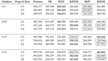 |
Table A3.
AIC Fit Statistics with Varying Parameters, a Fixed Sample Size of 200, and a Dispersion of 1.
Table A3.
AIC Fit Statistics with Varying Parameters, a Fixed Sample Size of 200, and a Dispersion of 1.
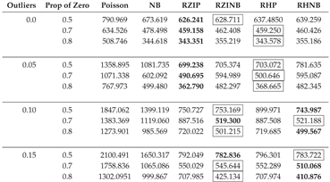 |
Table A4.
AIC Fit Statistics with Varying Parameters, a Fixed Sample Size of 500, and a Dispersion of 1.
Table A4.
AIC Fit Statistics with Varying Parameters, a Fixed Sample Size of 500, and a Dispersion of 1.
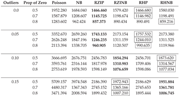 |
Table A5.
AIC Fit Statistics with Varying Parameters, a Fixed Sample Size of 50, and a Dispersion of 3.
Table A5.
AIC Fit Statistics with Varying Parameters, a Fixed Sample Size of 50, and a Dispersion of 3.
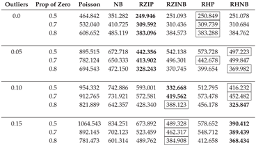 |
Table A6.
AIC Fit Statistics with Varying Parameters, a Fixed Sample Size of 200, and a Dispersion of 3.
Table A6.
AIC Fit Statistics with Varying Parameters, a Fixed Sample Size of 200, and a Dispersion of 3.
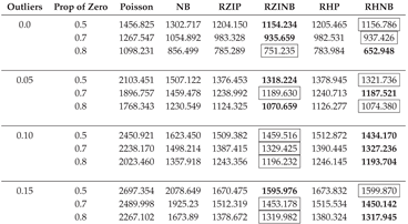 |
Table A7.
AIC Fit Statistics with Varying Parameters, a Fixed Sample Size of 500, and a Dispersion of 3.
Table A7.
AIC Fit Statistics with Varying Parameters, a Fixed Sample Size of 500, and a Dispersion of 3.
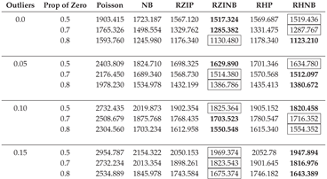 |
Table A8.
AIC Fit Statistics with Varying Parameters, a Fixed Sample Size of 50, and a Dispersion of 5.
Table A8.
AIC Fit Statistics with Varying Parameters, a Fixed Sample Size of 50, and a Dispersion of 5.
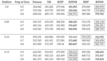 |
Table A9.
AIC Fit Statistics with Varying Parameters, a Fixed Sample Size of 200, and a Dispersion of 5.
Table A9.
AIC Fit Statistics with Varying Parameters, a Fixed Sample Size of 200, and a Dispersion of 5.
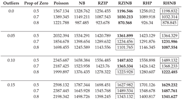 |
Table A10.
AIC Fit Statistics with Varying Parameters, a Fixed Sample Size of 500, and a Dispersion of 5.
Table A10.
AIC Fit Statistics with Varying Parameters, a Fixed Sample Size of 500, and a Dispersion of 5.
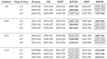 |
Table A11.
Model Estimation of Coefficients Using Robust Zero-Inflated Models.
| Parameter | RHP (Count Model) | RHNB (Count Model) | ||||||
|---|---|---|---|---|---|---|---|---|
| Estimate (SE) | P-Value | Estimate (SE) | P-Value | |||||
| Intercept | -0.8571 (0.1514) | <0.0001 | -1.0239 (0.3020) | <0.0001 | ||||
| BreachDelivery | 0.1159 (0.0496) | 0.0195 | 0.1467 (0.1250) | 0.2404 | ||||
| AssistedDeliveries | -0.0038 (0.0200) | 0.8504 | 0.0072 (0.0315) | 0.8193 | ||||
| EarlyTeenPreg | 0.0568 (0.0250) | 0.0232 | 0.1514 (0.0215) | <0.0001 | ||||
| LateTeenPreg | 0.0219 (0.0150) | 0.1443 | 0.0116 (0.0346) | 0.7376 | ||||
| Parameter | RHP (Zero Model) | RHNB (Zero Model) | ||||||
| Estimate (SE) | P-Value | Estimate (SE) | P-Value | |||||
| Intercept | -2.8706 (1.1909) | 0.0159 | -2.8867 (1.2799) | 0.0241 | ||||
| BreachDelivery | -0.1578 (0.4464) | 0.7238 | -0.08897 (0.5621) | 0.8742 | ||||
| AssistedDeliveries | -16.7361 (15.3676) | 0.2761 | -0.01931 (0.0747) | 0.7959 | ||||
| EarlyTeenPreg | 1.0192 (0.7228) | 0.1585 | 0.2751 (1.3401) | 0.8373 | ||||
| LateTeenPreg | 0.1195 (0.0464) | 0.0100 | 0.0700 (0.0699) | 0.3171 | ||||
Table A12.
Model Estimation of Coefficients Using Robust Hurdle Models.
| Parameter | RHP (Count Model) | RHNB (Count Model) | ||
|---|---|---|---|---|
| Estimate (SE) | P-Value | Estimate (SE) | P-Value | |
| Intercept | -0.8527 (0.2694) | 0.0016 | -0.8753 (0.3306) | 0.0081 |
| BreachDelivery | 0.1357 (0.0462) | 0.0033 | 0.1476 (0.1172) | 0.2080 |
| AssistedDeliveries | 0.0046 (0.0242) | 0.8491 | 0.0047 (0.0256) | 0.8534 |
| EarlyTeenPreg | 0.0539 (0.0273) | 0.0484 | 0.0547 (0.0320) | 0.0874 |
| LateTeenPreg | 0.0133 (0.0210) | 0.5263 | 0.0126 (0.0226) | 0.5770 |
| Parameter | RHP (Zero Model) | RHNB (Zero Model) | ||
| Estimate (SE) | P-Value | Estimate (SE) | P-Value | |
| Intercept | -0.5983 (0.1826) | 0.0011 | -0.4389 (0.2206) | 0.0421 |
| BreachDelivery | 0.1003 (0.1335) | 0.4529 | 0.0513 (0.0235) | 0.0582 |
| AssistedDeliveries | 0.0074 (0.0342) | 0.8275 | 0.0654 (0.0412) | 0.05827 |
| EarlyTeenPreg | -0.0943 (0.0507) | 0.0627 | -0.0853 (0.0761) | 0.7681 |
| LateTeenPreg | -0.0226 (0.0149) | 0.1308 | -0.0167 (0.0149) | 0.8135 |
References
- Shahsavari, S. Shahsavari, S. Robust Inference for Zero-Inflated Models with Outliers Applied to the Number of Involved Lymph Nodes in Patients with Breast Cancer 2023.
- Feng, C.X. A comparison of zero-inflated and hurdle models for modeling zero-inflated count data. Journal of statistical distributions and applications 2021, 8, 8. [Google Scholar] [CrossRef] [PubMed]
- Lambert, D. Zero-inflated Poisson regression, with an application to defects in manufacturing. Technometrics 1992, 34, 1–14. [Google Scholar] [CrossRef]
- Min, Y.; Agresti, A. Random effect models for repeated measures of zero-inflated count data. Statistical modelling 2005, 5, 1–19. [Google Scholar] [CrossRef]
- Hall, D.B. Robust estimation for zero-inflated Poisson regression. Scandinavian Journal of Statistics 2010, 37, 237–252. [Google Scholar] [CrossRef]
- Mullahy, J. Specification and testing of some modified count data models. Journal of econometrics 1986, 33, 341–365. [Google Scholar] [CrossRef]
- Tüzen, F. A simulation study for count data models under varying degrees of outliers and zeros. Communications in Statistics - Simulation and Computation 2018, 49, 1078–1088. [Google Scholar] [CrossRef]
- Tawiah, K.; Iddi, S.; Lotsi, A. On Zero-Inflated Hierarchical Poisson Models with Application to Maternal Mortality Data. International Journal of Mathematics and Mathematical Sciences 2020, 2020, 1407320. [Google Scholar] [CrossRef]
- Bassey, U.E.; Akinyemi, M.I.; Njoku, K.F. On Zero inflated models with applications to maternal healthcare utilization. International Journal of Mathematical Sciences and Optimization: Theory and Applications 2021, 7, 65–75. [Google Scholar] [CrossRef]
- Abonazel, M.R.; El-sayed, S.M.; Saber, O.M. Performance of robust count regression estimators in the case of overdispersion, zero inflated, and outliers: simulation study and application to German health data. Commun. Math. Biol. Neurosci. 2021, 2021, Article-ID. [Google Scholar]
- Adehi, M.; Yakasai, A.; Dikko, H.; Asiribo, E.; Dahiru, T. Risk of maternal mortality using relative risk ratios obtained from poisson regression analysis. International Journal of Development Research 2017, 7, 15405–15409. [Google Scholar]
- Okello, S.; Otieno Omondi, E.; Odhiambo, C.O. Improving performance of hurdle models using rare-event weighted logistic regression: an application to maternal mortality data. Royal Society Open Science 2023, 10, 221226. [Google Scholar] [CrossRef]
- Chau, A.M.H.; Lo, E.C.M.; Wong, M.C.M.; Chu, C.H. Interpreting poisson regression models in dental caries studies. Caries Research 2018, 52, 339–345. [Google Scholar] [CrossRef] [PubMed]
- Shahsavari, S.; Moghimbeigi, A.; Kalhor, R.; Jafari, A.M.; Bagherpour-kalo, M.; Yaseri, M.; Hosseini, M. Zero-Inflated Count Regression Models in Solving Challenges Posed by Outlier-Prone Data; an Application to Length of Hospital Stay. Archives of Academic Emergency Medicine 2024, 12, e13–e13. [Google Scholar] [PubMed]
- Huber, P.J. Robust estimation of a location parameter. In Breakthroughs in statistics: Methodology and distribution; Springer, 1992; pp. 492–518.
- Cantoni, E.; Zedini, A. A robust version of the hurdlemodel. Journal of Statistical Planning and Inference 2011, 141, 1214–1223. [Google Scholar] [CrossRef]
- Miranda, M.; Miranda, M.C.; Gomes, M.I. A robust hurdle poisson model in the estimation of the extremal index. Springer Proceedings in Mathematics &Amp; Statistics 2022, pp. 15–28. [CrossRef]
- Hamura, Y.; Irie, K.; Sugasawa, S. Robust hierarchical modeling of counts under zero-inflation and outliers. arXiv preprint arXiv:2106.10503 2021.
- Akaike, H. A new look at the statistical model identification. IEEE transactions on automatic control 1974, 19, 716–723. [Google Scholar] [CrossRef]
- Vuong, Q. Likelihood ratio tests for model selection and non-nested hypotheses. Econometrica 1989, 57, 307. [Google Scholar] [CrossRef]
Figure 1.
Graphicical Representation of Multicollinearity.
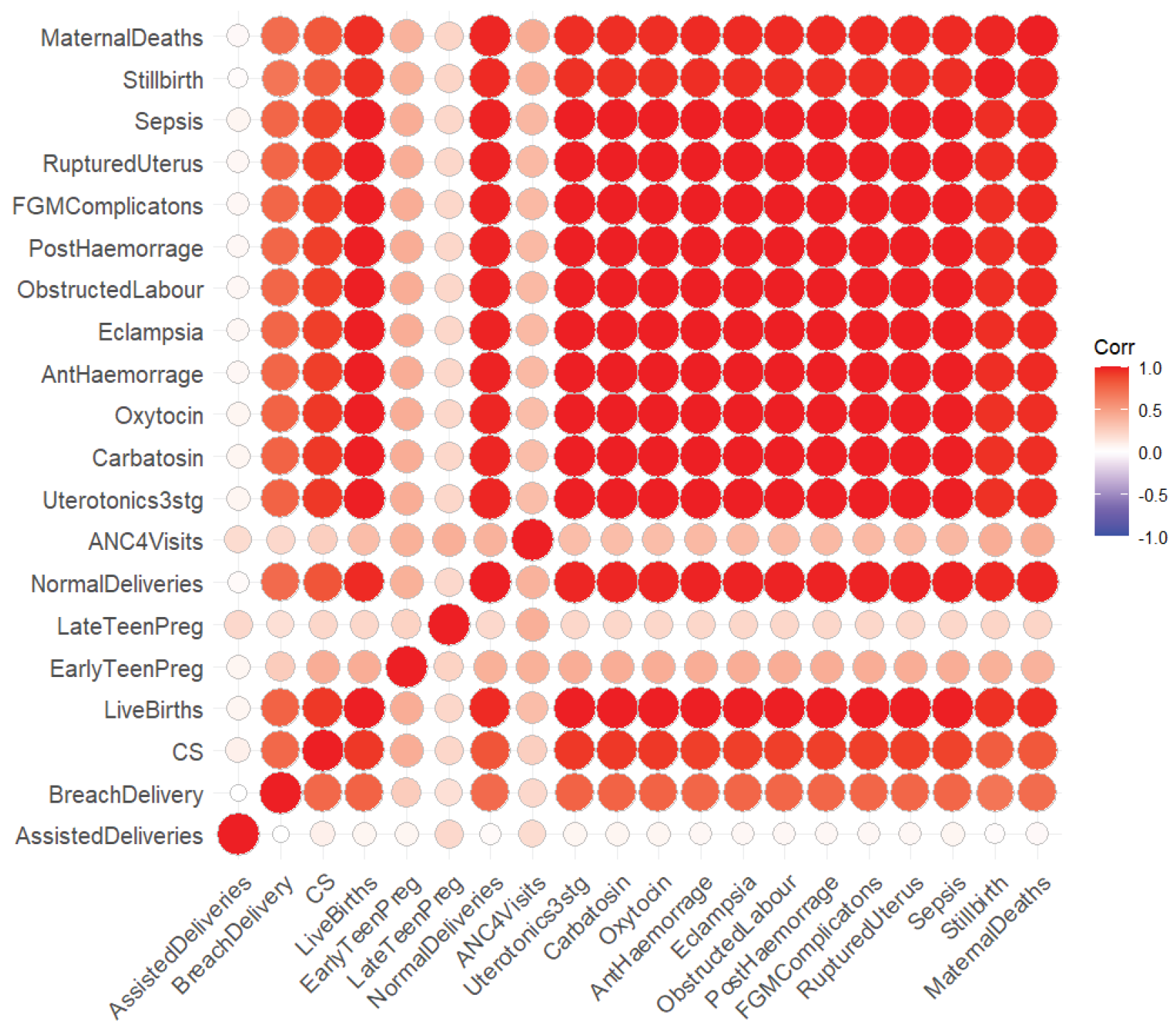
Figure 2.
Reduced Correlated Variables.
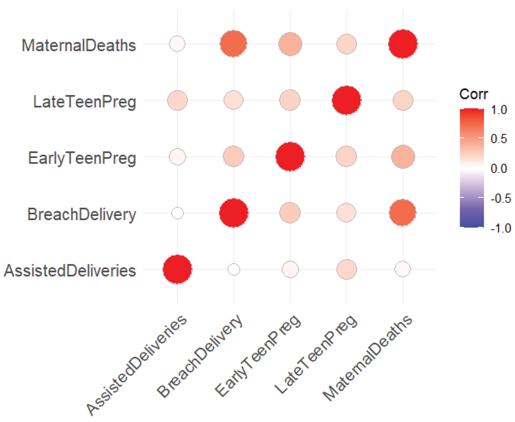
Figure 3.
Probability Models for the Number of Maternal Deaths.
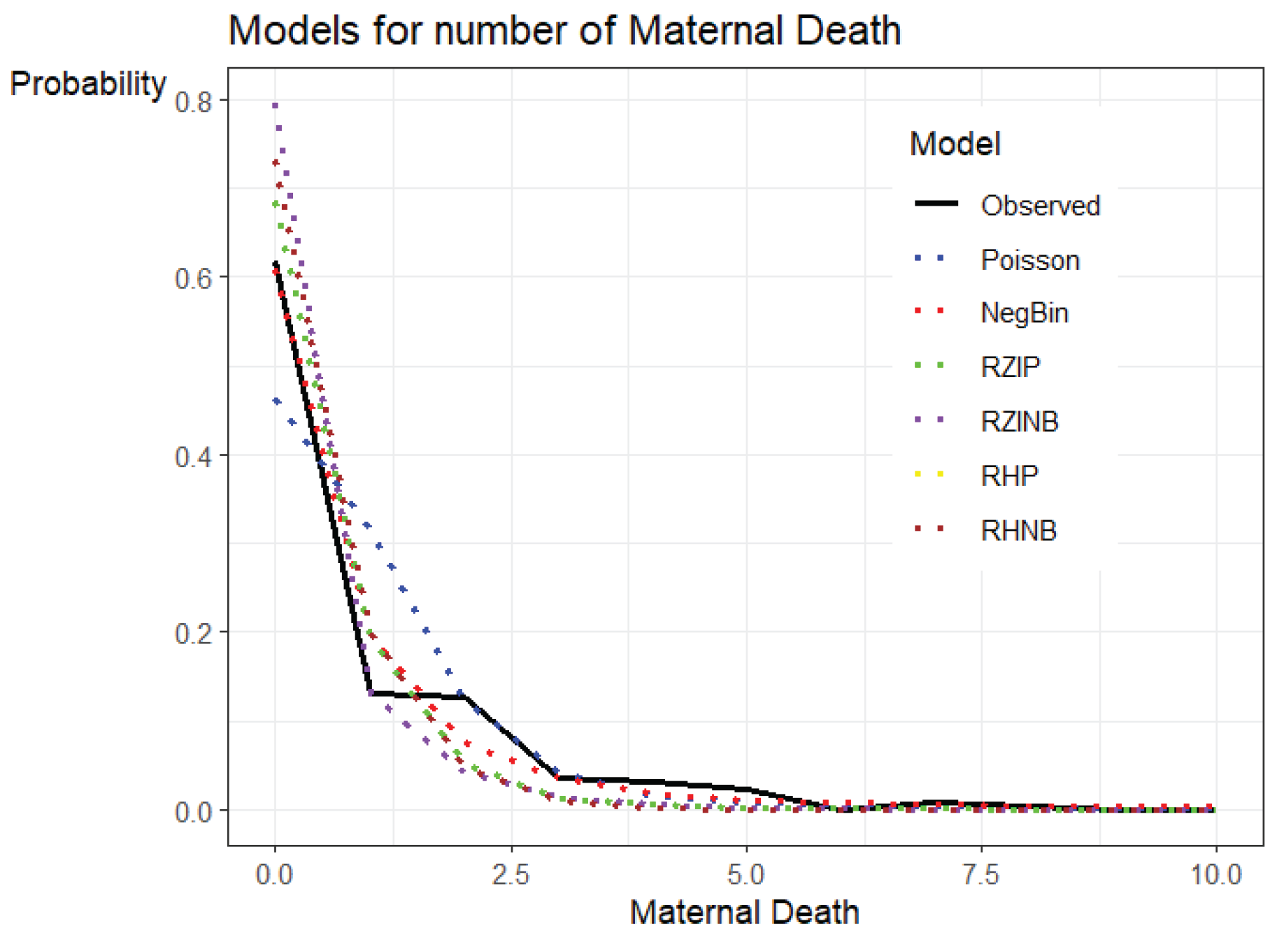
Table 1.
Simulation Scenarios Considered in the Simulation Study.
| Sample Size | Prop of Zeros | Dispersion | Outliers |
|---|---|---|---|
| 0.00 | |||
| 50 | 0.5 | 1 | 0.05 |
| 200 | 0.7 | 3 | 0.10 |
| 500 | 0.8 | 5 | 0.15 |
Table 2.
Correlation Matrix of Selected Variables
| Assisted | Breach | EarlyTeen | LateTeen | MaternalDeaths | |
|---|---|---|---|---|---|
| AssistedDeliveries | 1.000 | 0.001 | 0.064 | 0.199 | 0.035 |
| BreachDelivery | 0.001 | 1.000 | 0.264 | 0.157 | 0.734 |
| EarlyTeenPreg | 0.064 | 0.264 | 1.000 | 0.235 | 0.388 |
| LateTeenPreg | 0.199 | 0.157 | 0.235 | 1.000 | 0.222 |
| MaternalDeaths | 0.035 | 0.434 | 0.388 | 0.222 | 1.000 |
Table 3.
Clinical Characteristics of the Study Population.
| Factors | No death reported(%) | Death reported (%) |
|---|---|---|
| Assisted Delivery | 28.79 | 71.21 |
| Breech Delivery | 52.69 | 47.31 |
| Early Teen Pregnancy | 25.42 | 74.58 |
| Late Teen Pregnancy | 50.88 | 49.12 |
Table 4.
Vuong Test Comparison for Different Models.
| Model | RZIP | RZINB | RHP | RHNB | POIS | NB | Best Model |
|---|---|---|---|---|---|---|---|
| RZIP | 0.004*** | 0.002 *** | 0.003*** | 0.002*** | 0.000*** | RZIP | |
| RZINB | 0.012** | 0.011** | 0.000 *** | 0.000 *** | RZINB | ||
| RHP | 0.011** | 0.003*** | 0.002*** | RHP | |||
| RHNB | 0.003*** | 0.003*** | RHNB | ||||
| POIS | 0.003*** | NB | |||||
| NB |
***p < 0.001, ** p < 0.01
Table 5.
Estimated AIC and BIC for the Maternal Mortality data.
| Model | AIC | BIC |
|---|---|---|
| Poisson | 660.2816 | 677.2950 |
| NB | 554.6014 | 575.0174 |
| RZIP | 366.8992 | 400.9260 |
| RZINB | 395.2032 | 432.6327 |
| RHP | 372.6716 | 406.6984 |
| RHNB | 374.6517 | 412.0811 |
Table 6.
Model Estimation of Coefficients Using Robust Zero-Inflated Models.
| Parameter | RZIP (Count Model) | RZIP (Zero Model) | ||||
|---|---|---|---|---|---|---|
| Estimate (SE) | P-Value | Estimate (SE) | P-Value | |||
| Intercept | -0.8571 (0.1514) | <0.0001 | -2.8706 (1.1909) | 0.0159 | ||
| BreachDelivery | 0.1159 (0.0496) | 0.0195 | -0.1578 (0.4464) | 0.7238 | ||
| AssistedDeliveries | -0.0038 (0.0200) | 0.8504 | -16.7361 (15.3676) | 0.2761 | ||
| EarlyTeenPreg | 0.0568 (0.0250) | 0.0232 | 1.0192 (0.7228) | 0.1585 | ||
| LateTeenPreg | 0.0219 (0.0150) | 0.1443 | 0.1195 (0.0464) | 0.0100 | ||
Table 7.
Model Validation Results.
| Statistic | Value |
|---|---|
| Chi-Square Statistic | 20809.280 |
| Degrees of Freedom | 6.000 |
| P-value | 0.198 |
Table 8.
Likelihood Ratio Test Results.
| Comparison | df1 | df2 | LogLik1 | LogLik2 | Chisq | p-value |
|---|---|---|---|---|---|---|
| ZIP vs RZINB | 10 | 11 | -173.45 | -186.60 | 26.304 | 0.09 |
| RZIP vs RHP | 10 | 10 | -173.45 | -176.34 | 5.7724 | 0.06 |
| RZIP vs RHNB | 10 | 11 | -173.45 | -176.33 | 5.7525 | 0.47 |
Disclaimer/Publisher’s Note: The statements, opinions and data contained in all publications are solely those of the individual author(s) and contributor(s) and not of MDPI and/or the editor(s). MDPI and/or the editor(s) disclaim responsibility for any injury to people or property resulting from any ideas, methods, instructions or products referred to in the content. |
© 2025 by the authors. Licensee MDPI, Basel, Switzerland. This article is an open access article distributed under the terms and conditions of the Creative Commons Attribution (CC BY) license (http://creativecommons.org/licenses/by/4.0/).
Copyright: This open access article is published under a Creative Commons CC BY 4.0 license, which permit the free download, distribution, and reuse, provided that the author and preprint are cited in any reuse.


