Submitted:
05 June 2025
Posted:
06 June 2025
You are already at the latest version
Abstract
Elasticity is a well-established field within mathematical physics, yet new formulations can provide deeper insight and computational advantages. This study explores the geometry of two- and three-dimensional elastic curves using the formalism of Geometric Algebra, offering a unified and coordinate-free approach. The work systematically derives the Frenet, Darboux, and Bishop frames within the three-dimensional Geometric Algebra and employs them to integrate the elastica equation. A concise Lagrangian formulation is introduced, enabling the identification of Noetherian, conserved, multivector moments associated with the elastic system. A particularly compact form of the elastica equation emerges when expressed in the Bishop frame, revealing structural simplifications and making the equations more amenable to analysis. Ultimately, the Geometric Algebra perspective uncovers a natural correspondence between the theory of free elastic curves and classical beam models, showing how constrained theories, such as Euler-Bernoulli and Kirchhoff beam formulations arise as special cases. These results not only clarify foundational aspects of elasticity theory but also provide a framework for future applications in continuum mechanics and geometric modeling.
Keywords:
Geometric Algebra
; Clifford Algebra
; Bishop frame
; Frenet frame
; Darboux frame
; Kirchhoff Beam Theory
Elasticity is a mature branch of mathematical physics. The foundations of nonlinear beam models date back to Euler’s elastica, which describes planar beams undergoing bending deformations, and were later extended by Kirchhoff to spatial beams having torsional deformations. The closed-form solutions for the elastica, initially derived by Saalschütz in 1880 [1], rely on the theory of the Jacobi elliptic functions [2]. A recent account can be found in [3].
Kirchhoff discovered that the equilibrium equations for a straight, prismatic, and unstressed elastic rod are analogous to the equations for a spinning top [4,5]. These results suggest that the kinetic analogy was a useful guideline in obtaining solutions [4]. The classical approach by Love [4] adopted a Lagrangian approach, characterizing a filament by contiguous cross-sections that remain undeformed, perpendicular to the rod’s center-line, and capable of rotating relative to each other. Under the assumptions of Love, the static beam theory is equivalent to the description of an elastic curve attached to the center line of the beam.
The present contribution nevertheless will put a different perspective on the study of the elastic curves in 2 and 3 spatial dimensions. The presented approach can be extended to a higher number of dimensions since the applied formalism is dimension co-variant. That is, the applied methodology can be extend in a straightforward and almost algorithmic manner if one wishes to apply it to higher-dimensional problems. This generality is achieved by employing the apparatus of Geometric Algebra.
The main contribution of the paper is the coordinate-free expression of the elastica equation using only the curvature and the local inertial reference frame (i.e. the Bishop frame). The paper is organized as follows. Section 1 introduces the main concepts of Geometric Algebra. Section 2 introduces the Frenet, Gradient and Bishop frames. Section 3 develops the Euler-Lagrange theory of the elastica. Section 4 discusses the main applications of the theory.
1. Geometric Algebra
In the following section we use the convention of denoting the scalars with Greek letters, the vectors with lowercase Latin letters, and multi-vectors and blades with capital Latin letters. The planar Euclidean geometric algebra is generated by the set of orthonormal basis vectors for which the so-called geometric product is defined with properties
The pseudoscalar is denoted by . The structure of the algebra can be illustrated in the diagram below
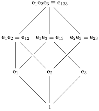 |
Blades are also denoted by index concatenation as above. An overview of the topic, including its applications to physics, can be found in the books of MacDonald [6] and Hestenes [7], Doran and Lasenby [8].
1.1. Products in GA
The geometric product of two vectors can be decomposed into a symmetrical scalar product and an antisymmetrical wedge product:
The wedge product is called also exterior by some authors. For higher-dimensional objects, the scalar product is defined simply as the scalar part of the geometric product between multivectors:
where the notation 〈〉k denotes the part of the multivector of grade k.
Furthermore, the wedge product is extended for blades (products of basis vectors) as
The interior product, called sometimes also Hestenes contraction (see the discussion in [12]), is a symmetrical operation defined for multi-vectors of grades r and l, respectively, as
while for scalars . Therefore, for vectors as expected from the vector calculus.
It is noteworthy also that for a vector and a blade [9] [Ch. 1, p.3]
which extends the geometric product decomposition also to the products of vectors and blades:
It should be noted that unlike the scalar product the contraction is not associative in the general case.
The cross product for the 3 dimensional space can be expressed as
1.2. Principal Automorphisms
Three principle automorphisms can be identified in Geometric Algebra:
- vector reflection:
- geometric product reversion:
- inverse blade, or Hermite, automorphism (IBA): , for the respective blade
While the first two automorphisms are broadly recognized, the third one is appreciated less. The IBA is obviously defined only for non-nilpotent blades. Technically speaking, the reversion and IBA are anti-automorphisms [10].
1.3. Norm
For Clifford algebras with unspecified signatures the norm of a multivector can be defined as
For vectors we have the special case , which reminds of the formula for the absolute value of a scalar. For positive signatures, i.e. for , we have the equivalent formula
1.4. Elements of Geometric Calculus
The geometric derivative subsumes divergence, curl and gradient operations of the vector calculus. Introduction on the topic can be found in [11]. It is defined in the simplest way as
where are the components of the dual or reciprocal basis, such that
for an arbitrary vector x. For the dual basis since , where the denotes the Kronecker’s symbol.
The geometric derivative is co-ordinate independent. Moreover, it splits into a grade-lowering and grade-increasing parts
Therefore, in many cases ∇ can be treated as a vector.
2. Frenet, Gradient and Inertial Frames in 3D
In the present section, the approach outlined above will be applied to the 3D Euclidean space. Differential geometry can be readily analyzed with the tools provided by geometric algebra. The approach pioneered by Hestenes, Sobczyk, Doran, and Lasenby is to use the shape operator as the main tool for the differential geometry described by the tools of the geometric algebra [7,8] [Ch. 6], [13]. It uses the tangent vectors on the surface to build the pseudoscalar at every point from the tangent vectors of the parameter curves on the surface. Although general in nature this approach can be simplified for curves and given explicit form for engineering and physical applications.
In the subsequent discussion we work in . The pesudoscalar is denoted by and it commutes with all elements of the algebra. Consider the scalar equation , which defines a surface in 3D. We can use it to specify also a vector field defining curve embedded in that surface in the following way.
Definition 1.
Define the curve specified by by the vector field , for which
for suitable functions , such that
holds identically.
Considering a curve in the 3D space, there is a parametrization by the length s, such that
The assumption here is that is non-singular except at . Then define the tangent vector as
Then
Therefore, the gradient is orthogonal to t. Furthermore,
We also obtain the equivalence
Furthermore, identically
2.1. Frenet Frames
Consider the normalization constraint . Differentiate the equation to obtain
Therefore, is orthogonal to t. Define the curve normal as
where the unsigned curvature is defined as the norm of the acceleration
Therefore, we can compute the signed curvature as and use this expression throughout. The bi-normal vector b is orthogonal to the osculating plane :
It also holds that
Define the torsion as
The torsion measures the amount of rotation of the Frenet frame around the tangent t as the arc length increases (see Figure 1). Differentiating orthogonality relations
yields the anti-symmetric frame coefficient matrix
The frame derivative can be computed concisely from the matrix equation
On the other hand, the following identity holds
Therefore, we can identify a frame bi-vector up to an orthogonal bi-vector B,
such that and . The bi-vector B can be completely specified as follows.
Proposition 1.
For the case of Frenet frame the Darboux or angular velocity bi-vector is
and its dual Darboux vector is
Proof.
To demonstrate the statement we compute first the inner product
Therefore,
Compute
□
Therefore, the trajectory can be recovered by quadrature starting from the integral
so that
Remark 1.
The analogy between the frame matrix and frame bi-vector is not complete. The frame matrix Ω is singular since . This is not the case for the frame bi-vector Ω since the product results in a scalar, which is also the determinant of the bi-vector, so that its inverse is
2.2. Gradient (Darboux) Frame
Define the surface normal vector as
Remark 2.
The above relationship defines the Gauss map of the surface :
Define the osculating plane by the bi-vector and the tangent plane by . Define the bi-normal vector b to be orthogonal to the osculating plane O:
Then . It also holds that
as before. Differentiating the orthogonality relations
yields anti-symmetric coefficient frame matrix as before.
We will look for a Darboux bi-vector as before starting from the identity
Then
such that so that
Consider the constraint equation
Therefore
Consider the bi-vector
On the other hand,
in terms of the dual vector. Therefore,
Furthermore,
Therefore, the Darboux vector is
Therefore,
However,
Therefore,
Therefore, is the Darboux bi-vector of the gradient frame.
Proposition 2.
For the case of Gradient frame the Darboux or angular velocity bi-vector is
Define the coefficients
To determine explicitly and we use the following approach. Define the unit vector (i.e. the Frenet normal)
Then also . On the other hand,
Therefore, and b are co-linear. Moreover, since both are unit vectors it follows that . Therefore, . Therefore, there are 2 possible combinations and . Considering the planar case we observe that the second option realizes. Therefore, .
Define the dual vector
Then
Therefore, n and are co-linear. Furthermore,
Therefore, and . Therefore,
To summarize, the Frenet and Gradient frames are related by the transformation
or in shortened matrix notation
From the above equation it is apparent that U is an orthogonal matrix – . The frame matrix is
The two frame matrices are related by:
Remark 3.
The name Darboux frame is justified since we can identify the plane as the surface "arena" where the equations evolve. Since the Darboux frame is represented by the matrix
Then for the plane ; so up to the orientation of the normal vector one can identify with .
The tangent field can be recovered by quadrature as
The gradient frame can be recognized as the Darboux frame for the plane, where the geodesic curvature .
Remark 4.
The gradient frame can be suitable for immersed elastic curves and also in the case where one wishes to characterize the interaction of the elastica with the medium. There, one could specify a normal forcing field as a constraint of the equations. Therefore, by duality, in a deformed body (under a strain field) the strength of interaction can be given by the value of .
2.3. Bishop (Inertial) Frames
The Bishop or parallel transport frame [14] is an alternative description that is well-defined even when the curve has vanishing acceleration. The Bishop frame is such that
and furthermore the frame matrix is computed as
To connect with the approach discussed so far we observe that
Therefore, one can posit the rotation relationship
for some phase function of the arc-length to be determined further. We look for a Darboux bi-vector of the form
Then
Furthermore
and finally
Therefore, we can conclude that and the Darboux bi-vector has the especially simple form [7, Ch. 6, p. 238]
To determine the function we proceed as follows. Using the Frenet frame we form the invariant volume:
Observe that
Then
Therefore, from eq. 30 it follows that
as also determined in [15]. In other words, is the integral or cumulative torsion. It is a multiple of the twisting number. Therefore, the frame matrix becomes
From this presentation it is apparent that geometric calculus streamlines calculations.
3. Euler-Lagrange Formulation of the Elastica Problem
A beam is defined to be a three-dimensional deformable body whose length is much larger than its other two dimensions. Such a body can be described by a curve threading its center line in and a cross section at every point of the curve whose intersection is precisely the barycenter of the section. A comprehensive variational analysis has been presented in [16].
3.1. Free Elastica Equations
The elastica theory is the oldest variational model of elastic rods. The core of the presented approach is coordinate free. The constrained Lagrangian energy density functional is identified as
where its independent variables are vectors and the multiplier is scalar while t is not assumed a priori to be the tangent field. This Lagrangian is manifestly translationally invariant. The above Lagrangian corresponds to the traditional definition given in [15,17] since
under nomralization. Furthermore assume that , . The tangent field and its derivative are varied independently. To enact the variations we use the generalized partial gradient operator:
The free elastica equation can be derived as follows. Observe the relations
Therefore, the Euler-Lagrange equations are
That is, up to sign it holds that
3.2. Symmetries of the Lagrangian
The first equation integrates to the constant vector field J, which is also the Noether current, such that
Furthermore, define the pseudoscalar
and differentiate it to obtain
using the equation of motion. Therefore, w is also constant. Denote its magnitude by . Observe that it is an invariant which does not depend on the used basis.
Furthermore, we establish the stronger result that
without explicitly using the dimensionality of Euclidean space. Therefore, we claim:
Proposition 3.
An elastica is confined to a 3 dimensional subspace of .
Therefore, without loss of generality we assume further that .
Furthermore, by the Ostrogradski principle for higher-order Lagrangians [18], the equation for the Hamiltonian is given by
Differentiate the Hamiltonian and use the equations of motion to obtain
by the orthogonality of t and . Therefore, it was just established that the Hamiltonian is a first integral of the system – i.e. a constant.
Furthermore, the conservation of the Hamiltonian can be interpreted as the energy conservation law for the elastic energy density:
applying the normalization of t and the definition of .
The torque can be identified with the bi-vector
relating to the Bishop frame bi-vector. Therefore,
is the expression of the conservation law of angular momentum. Therefore, can be identified with some constant M – i.e. .
Remark 5.
We can define the generalized, multi-vector Hamiltonian, which combines both conservation laws, as an even element of the algebra as
In this formulation, corresponds to a constant quaternion. Therefore, we have just established that an elastica can be suitably parametrizied, and therefore classified, by a quaternion up to a rigid motion.
Observe that
up to sign. Therefore, we can attribute the volumetric invariant to the torque.
Note that up to the last equation the approach is completely frame-independent! Thus, the choice of a specific frame and coordinates is a matter of utility guided by the need to simplify computations.
3.3. Derivation of the Curvature Equation
Observe that
Having derived the relevant symmetries of the system at this point we specialize the discussion and employ the Frenet frames to express J.
Therefore,
in the Frenet frame. The magnitude of the momentum vector can be calculated from the scalar product:
for some constant j giving the norm of J. Observe that the above equation is also frame-independent.
Furthermore, compute the pseudoscalar and identify the constraint
coupling curvature and torsion.
Lastly, the Lagrange multiplier’s functional form is determined in the following way. Project J onto the tangent vector to obtain:
Substitute in eq. 41 to obtain the Lagrange multiplier
Project J onto the normal vector to obtain:
Differentiate to obtain
Substitute from eq. 46 to obtain
agreeing with the result in [19].
Remark 6.
The traditional derivation of the elastic equation proceeds as follows [20]. Differentiate J and use the Frenet frame equations
to obtain a system of 3 constraints:
Solve the constraint for the torsion
and the Lagrange multiplier
Substitute the solutions in the remaining constraint. Observe that using the traditional approach the role of the constant H is not apparent.
The advantage of the geometric-algebraic approach is that one does not need to solve a differential equation for the torsion. Instead, the role of the invariant pseudoscalar is put to the front. From the present discussion it transpires that choice of frame is a matter of convenience for the problem at hand.
The preceding discussion can be formulated concisely as the following theorem:
Theorem 1.
The elastica system is equivalent to the first order ODE
which can be differentiated into the second order differential equation
where H is the Hamiltonian energy density of the system, c is the torsion coupling and j is the magnitude of the generalized momentum J. The vector field J can be expressed in the Frenet frame as
3.4. Classification of Elastic Curves
The torsion coupling condition requires some attention. On the first place,
Also . Therefore,
or equivalently,
in terms of the volume invariant. Therefore, in the non-trivial case, linear dependence between the 3 vectors () implies that the curve is planar (i.e. ). Let . Obviously, whenever t and are linearly dependent then . On the other hand, suppose that only . Then
While
Furthermore, is in the span of () since . The above results can be neatly summarized in the following diagram:
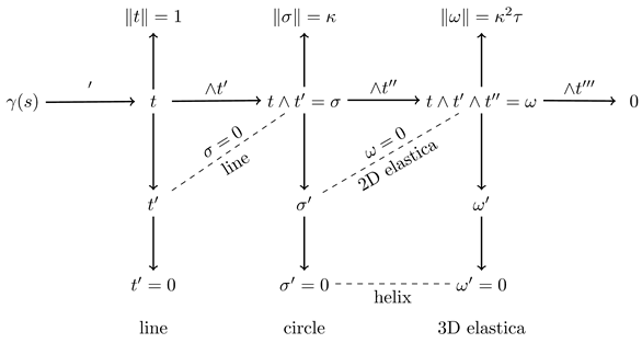 |
The above diagram is generated by the consecutive action of two operators – the covariant arc length differentiation and exterior multiplication.
4. Applications
4.1. Planar Elastica
Then . The curvature differential equation becomes
The equation is resolved by variation of parameters using the generic ansatz
This leads to the algebraic system for the parameters A, q and m:
This leads to a general solution of the form
The non trivial solutions are given by the set
Geometrically admissible are only the solutions where A is positive. This corresponds to the results given in [21] after a suitable reparametrization.
4.2. Generic 3D Elastica
We follow the method described in [20] where the equation is proven.
Proposition 4.
The substitution results in an autonomous ODE for u:
Proof.
Suppose that . Observe that wherever
Therefore,
and multiply by u. □
This equation can be integrated in elliptic functions as follows [15,19,22,23]. We make the ansatz
Observe that the 2D case corresponds to .
Using some identities for the elliptic functions, one arrives at the following system of polynomial equations for the parameters
Therefore, .
The last equation contains only the integration constants H, c and j besides the unknown parameter p. Therefore, the solutions can be parameterized by the roots of the equation for p. Then
and
This leads to a parametric solution of the form
In another parametrization we have the system of equations
which couples the p an q parameters algebraically. The advantage here is the linear relationship between p and H. The positive solution is
The denominator is always positive. Then the solutions are parametrized by the value of m. In the 2D case, as observed
Otherwise,
Remark 7.
The torsion is
which determines the Frenet frame. This can be integrated into an incomplete elliptical integral of the third kind.
allowing for calculation of the Bishop frame.
4.3. Integration of the Elastica in Terms of the Bishop Frame
Observe that equation 38 can be integrated as
Adding both conservation laws allows one to solve for the field using the invertivbility of the geometric product:
Observe, that the above formulation is coordinate-free demonstrating the advantage of Geometric Algebra approach. Therefore, we establish that the elastica is a completely integrable system in terms of the Bishop frame.
The conserved momentum allows for aligning the solution to a global basis and identifying a corresponding coordinate system. Such a convenient coordinate system is the cylindrical [19,22] one aligned with the momentum J (see Figure 2). We define the constant altitude unit vector along the direction of J as
In summary, we can formulate following result:
Theorem 2.
Suppose that the Bishop frame , j, H, M and are specified. Then the elastica curve can be reconstructed by quadrature as:
under the compatibility condition
Proof.
Consider the identity (eq. 39). Therefore, we are led to a new equation in terms of the preferred direction, which splits into translational and rotational components as follows:
Furthermore, the first term can be interpreted as a sum of translations, while the second term – as a sum of rotations.
Eq. 69 implies the compatibility condition
Therefore, formally the Bishop frame can be determined by quadrature as
from the tangent field, so the total angular momentum can be identified with the integration constant of the Bishop frame. □
Geometrically eq. 71 amounts to establishing a preferred orientation of the system (i.e. a global cylindrical symmetry). Using these coordinates, the solutions can be represented conveniently in a cylindrical coordinate system [22]. Then for the altitude we have
So we can identify the altitude (i.e. the z-axis) with the direction of translation. Using eq. 63 one obtains directly
in terms of the Jacobi epsilon function.
Consider the identity
We can solve for the radial component as
To obtain the angular coordinate proceed as follows and furthermore,
Differentiate eq. 73 as
Take the inner products
Integrate to obtain the polar coordinates
The procedure can be explicated in the next section.
4.4. Construction of the Preferred Coordinate System
The exposition follows the approach of [22] taking into account the differences in the employed formalism.
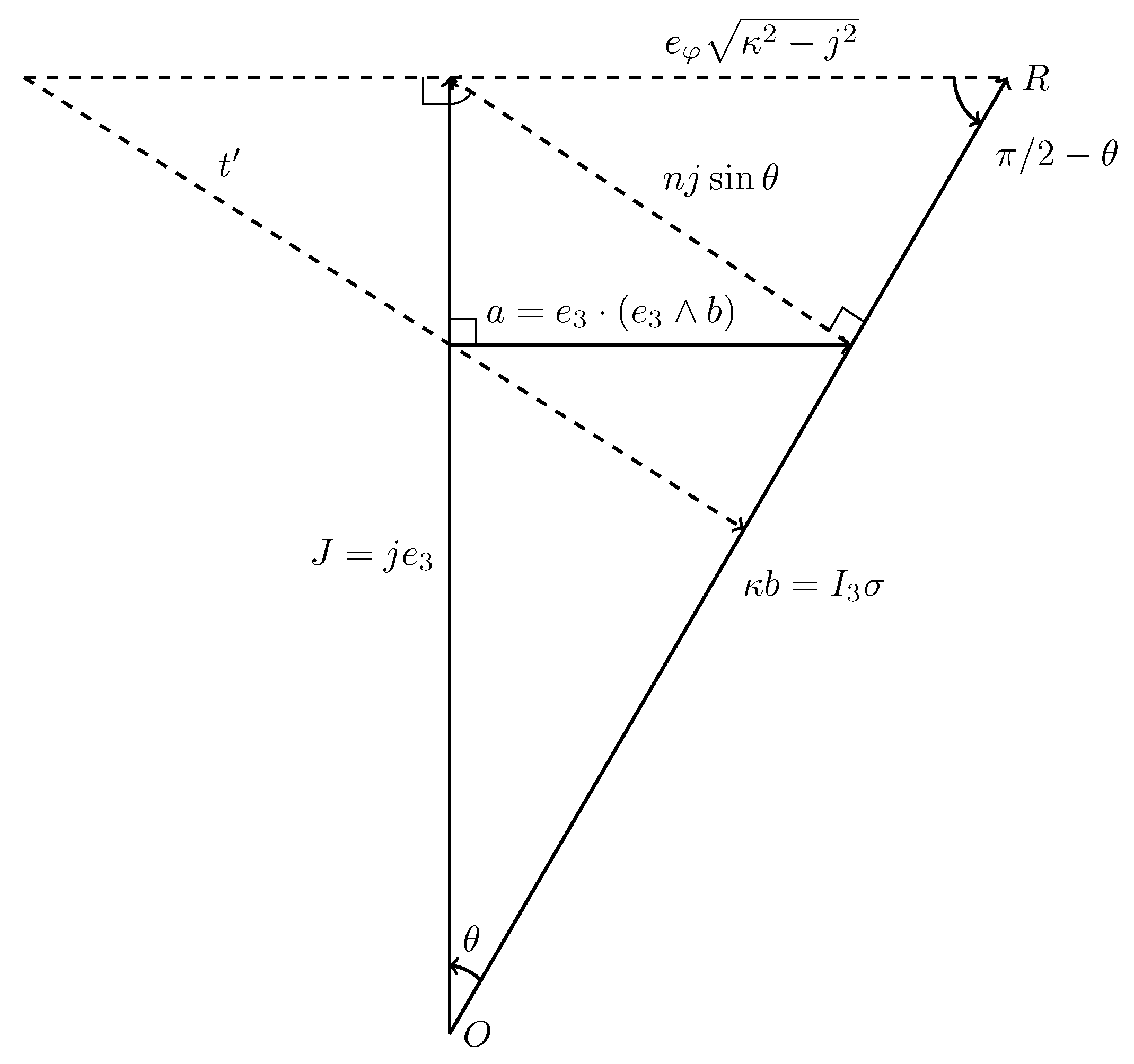
Observe that so that (see Figure 2). The solid angle between the planes and is given by
To construct compute the rejection vector to b in the plane (see Figure 3)
Furthermore, we have the identity
Therefore, the norm of the vector a can be computed as
after substitution in eq. 43 since .
Observe that in cylindrical coordinates
The two remaining coordinate equations can be obtained as the scalar products
Direct representation of a in terms of the Frenet frame using eq. 50 results in
Furthermore, the third basis vector can be computed as .
Then
so that
Therefore,
from eqs. 76 and 79, which directly integrates to
Furthermore,
so that
This can be integrated into
in terms of the incomplete elliptic integral of the 3rd kind, corresponding to the result in [24]. This is, however, not the most convenient representation as noted in [23]. It is produced here only to demonstrate the correspondence of the approach.
4.5. Specialization to 2D
To connect with the 2D application we use the frames {} with pseudoscalar . Observe that the Bishop frame is simply and the torque bi-vector is .
Then one immediately obtains the solution
Furthermore, the linear momentum becomes
Example 1.
One of the solutions are the set of equations
5. Discussion
The present contribution considers the problem of 2D and 3D non-extendable elastic beams and rods from the perspective of Geometric algebra. This allows for a great simplification of the problem due to the considerable expression power of the Geometric algebra approach. Notably, the approach obviates the use of a non-Euclidean configuration space [5]. Instead, all calculations are performed in the physical Euclidean space.
The paper demonstrates the forms of Frenet, Darboux, and Bishop frames in . It furthermore offers a new Lagrangian formulation of the elastica theory. This allows for construction of the fundamental Notherian conserved quantities. The Geometric algebra approach also enables an intuitive classification of the elastica system using its geometric invariants.
Concise expressions of the elastica equations are found using the Bishop frame. The Geometric algebra approach demonstrates natural correspondence of the free elastic problem with the Kirchhoff beam theory. Finally, we have determined a coordinate-free formulation of the solution.
Possible applications of the approach are inverse problems, image analysis and Finite Element Modeling, FEM.
Funding
The present work was funded by the European Union’s Horizon Europe program under grant agreement VIBraTE 101086815.
Conflicts of Interest
The authors declare no conflicts of interest. The funders had no role in the design of the study; in the collection, analyses, or interpretation of data; in the writing of the manuscript; or in the decision to publish the results.
Abbreviations
The following abbreviations are used in this manuscript:
| FEM | Finite Element Modeling |
| GA | Geometric Algebra |
| IBA | Inverse Blade Automorphism |
| ODE | Ordinary Differential Equation |
Appendix A. Elliptic Integrals and Functions
Appendix A.1. Elliptic Integrals of the First Kind
Incomplete elliptic integral of the 1st kind:
The Jacobi amplitude function is the inverse of the integral:
Its derivative is denoted by :
Therefore, we have the identity
The complete elliptic integral is defined as
The elliptic sine and cosine are defined by
Therefore, we have the identity
Appendix A.2. Elliptic Integrals of the Second Kind
Incomplete elliptic integral of the 2nd kind:
The complete elliptic integral is defined as .
The Jacobi epsilon function is defined as
The epsilon function is related to the incomplete elliptic integral of the 2nd kind as
Appendix A.3. Elliptic Integrals of the Third Kind
The incomplete elliptic integral of the third kind is given by
Furthermore, the integral can be analytically continued to a quasi-periodic function as
where denotes the fractional part of modulo . The integral is related to the elliptic functions by the integral equation
This formula follows from the substitution so that in the original argument. Therefore, we have also the formula
The complete elliptic integral of the third kind is given by
Appendix A.4. Integral Identities
References
- Saalschütz, L. Der belastete Stab unter Einwirkung einer seitlichen Kraft; B. G. Teubner: Leipzig, 1880. [Google Scholar]
- Greenhill, A.G. The applications of elliptic functions; Macmillan & co: London, 1892. [Google Scholar]
- Levien, R. The elastica: a mathematical history. Technical Report UCB/EECS-2008-103, 2008.
- AEH, L. A treatise on the mathematicaltheory of elasticity; Cambridge University Press: Cambridge, 1906. [Google Scholar]
- Greco, L.; Cuomo, M. Consistent tangent operator for an exact Kirchhoff rod model. Continuum Mechanics and Thermodynamics 2014, 27, 861–877. [Google Scholar] [CrossRef]
- MacDonald, A. Linear and Geometric Algebra; CreateSpace Independent Publishing Platform, 2010; p. 223. [Google Scholar]
- Hestenes, D.; Sobczyk, G. Clifford Algebra to Geometric Calculus; Springer: Netherlands, 1984. [Google Scholar] [CrossRef]
- Doran, C.; Lasenby, A. Geometric Algebra for Physicists; Cambridge University Press, 2003; p. 592. [Google Scholar]
- Hestenes, D. Space-Time Algebra, 2nd ed.; Birkhäuser: Basel, 2015; ISBN 978-3-319-18413-5. [Google Scholar]
- Chappell, J.M.; Iqbal, A.; Gunn, L.J.; Abbott, D. Functions of Multivector Variables. PLOS ONE 2015, 10, e0116943. [Google Scholar] [CrossRef] [PubMed]
- MacDonald, A. Vector and Geometric Calculus; CreateSpace, 2012. [Google Scholar]
- Dorst, L. The Inner Products of Geometric Algebra. In Applications of Geometric Algebra in Computer Science and Engineering; Dorst, L., Doran, C., Lasenby, J., Eds.; Birkhäuser: Boston, MA, 2002; pp. 35–46. [Google Scholar] [CrossRef]
- Hestenes, D. The Shape of Differential Geometry in Geometric Calculus. In Guide to Geometric Algebra in Practice; Springer: London, 2011; pp. 393–410. [Google Scholar] [CrossRef]
- Bishop, R.L. There is More than One Way to Frame a Curve. Amer. Math. Monthly 1975, 82, 246–251. [Google Scholar] [CrossRef]
- Langer, J.; Singer, D.A. Lagrangian Aspects of the Kirchhoff Elastic Rod. SIAM Review 1996, 38, 605–618. [Google Scholar] [CrossRef]
- Romero, I.; Gebhardt, C.G. Variational principles for nonlinear Kirchhoff rods. Acta Mech. 2019, 231, 625–647. [Google Scholar] [CrossRef]
- Singer, D.A.; Garay, O.J.; García-Río, E.; Vázquez-Lorenzo, R. Lectures on Elastic Curves and Rods. In Proceedings of the AIP Conference; 2008; Vol. 1002, pp. 3–32. [Google Scholar] [CrossRef]
- Rashid, M.S.; Khalil, S.S. Hamiltonian Description Of Higher Order Lagrangians. Int. J. Modern Phys. A 1996, 11, 4551–4559. [Google Scholar] [CrossRef]
- Langer, J.; Singer, D.A. Knotted Elastic Curves in R 3. Journal of the London Mathematical Society 1984, s2-30, 512–520. [Google Scholar] [CrossRef]
- Langer, J.; Singer, D.A. The total squared curvature of closed curves. J. Differential Geom. 1984, 20. [Google Scholar] [CrossRef]
- Djondjorov, P.; Hadzhilazova, M.; Mladenov, I.M. Explicit Parameterization of Euler’s Elastica. In Proceedings of the 9th International Conference on Geometry, Integrability and Quantization; Softex, 2008; pp. 175–186. [Google Scholar] [CrossRef]
- Shi, Y.; Hearst, J.E. The Kirchhoff elastic rod, the nonlinear Schrödinger equation, and DNA supercoiling. J. Chem. Phys. 1994, 101, 5186–5200. [Google Scholar] [CrossRef]
- Ameline, O.; Haliyo, S.; Huang, X.; Cognet, J.A.H. Classifications of ideal 3D elastica shapes at equilibrium. Journal of Mathematical Physics 2017, 58. [Google Scholar] [CrossRef]
- Tobias, I.; Coleman, B.D.; Olson, W.K. The dependence of DNA tertiary structure on end conditions: Theory and implications for topological transitions. The Journal of Chemical Physics 1994, 101, 10990–10996. [Google Scholar] [CrossRef]
Figure 1.
Frenet frame of a curve.
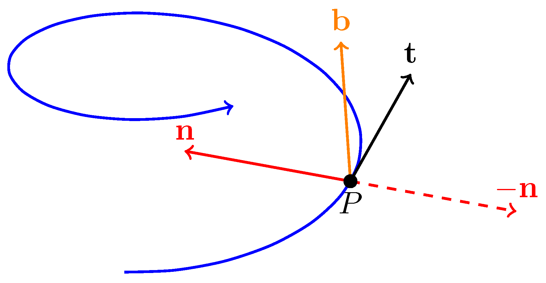
Figure 2.
The preferred coordination system and Bishop frame configuration.
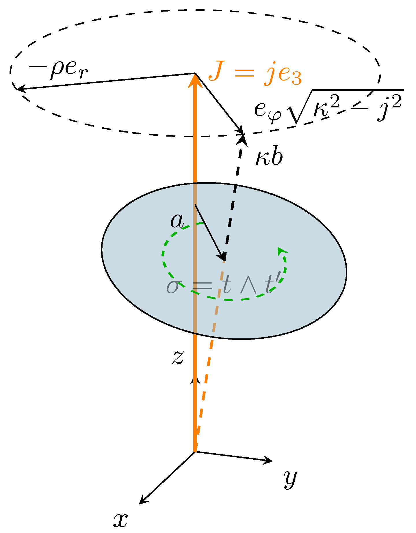
Figure 3.
A section of the preferred coordination system with the Bishop frame.
Disclaimer/Publisher’s Note: The statements, opinions and data contained in all publications are solely those of the individual author(s) and contributor(s) and not of MDPI and/or the editor(s). MDPI and/or the editor(s) disclaim responsibility for any injury to people or property resulting from any ideas, methods, instructions or products referred to in the content. |
© 2025 by the authors. Licensee MDPI, Basel, Switzerland. This article is an open access article distributed under the terms and conditions of the Creative Commons Attribution (CC BY) license (http://creativecommons.org/licenses/by/4.0/).
Copyright: This open access article is published under a Creative Commons CC BY 4.0 license, which permit the free download, distribution, and reuse, provided that the author and preprint are cited in any reuse.


