New Boundary Harnack Principles for Divergence Form Elliptic Equations with Right Hand Side

1. Introduction

1.1. Background

In this paper, we study boundary Harnack principles for divergence form equations with right hand side. Boundary Harnack principles originally state that, if u and v are two positive harmonic functions in $\Omega \cap B_1$, and they both vanish on $\partial \Omega \cap B_1$, then they are comparable near the boundary $\partial \Omega$.

For elliptic equations without right hand side in Lipschitz domains, we introduce some related research results. Kemper initially proved boundary Harnack principles for harmonic functions by applying the uniqueness of the positive singularity principle and the properties of Kernel functions in [24], while Caffarelli, Fabes, Mortola and Salsa first proved boundary Harnack principles for divergence form operators with bounded measurable coefficients in [8]. In [18], Fabes, Garofalo, Marin-Malave, and Salsa extensively discussed the non-divergence form operators by Fatou theorems. In [23], Jerison and Kenig extended boundary Harnack principles for divergence form operators in non-tangentially accessible domains. Bass and Burdzy proved boundary Harnack principles for non-divergence form elliptic operators with bounded measurable coefficients by applying probabilistic techniques in [5]. More recently, De Silva and Savin discovered a simple yet unified proof of divergence and non-divergence form operators with bounded measurable coefficients in their work published in [13].

For elliptic equations with right hand side in Lipschitz domains, we present some relevant results. In [1], Mark Allen and Shahgolian proved boundary Harnack principles of the Laplace operators by using harmonic functions in spherical polar coordinates under polynomial decaying conditions of the right hand side. In [31], Ros-Oton and Torres-Latorre already proved boundary Harnack principles for divergence form operators with continuous coefficients and non-divergence form operators with bounded measurable coefficients. In addition, Ros-Oton and Torres-Latorre gave a counterexample to show that boundary Harnack principles do not hold in ${\mathbb{R}}_{+}^2$ for divergence form operators with bounded measurable coefficients, even though the $L^q$ norm of the right hand side is controlled by a sufficiently small constant $c_0$.

For elliptic equations without right hand side in Hölder domains, we introduce some related background and research results. Boundary Harnack principles for non-divergence form operators in Hölder domains with the exponent $\alpha \in \left(\frac{1}{2},1\right]$ were first proven by Banuelos, Bass and Burdzy in [5] Bass1994. Fausto Ferrari first proved boundary Harnack principles for divergence form operators in Hölder domains with exponent $\alpha \in \left(0,1\right]$ in [19]. De Silva and Savin proved boundary Harnack principles for divergence and non-divergence form operators in Hölder domains with exponent $\alpha \in \left(\frac{1}{2},1\right]$ by using a simpler method in [13]. Further, in [14], De Silva and Savin, by optimizing the previous approach, generalize this theory in Hölder domains with exponent $\alpha \in \left(0,1\right]$.

Based on our current investigation and understanding, boundary Harnack principles for elliptic equations with right hand side in Hölder domains has not been fully studied. In [31], Ros-Oton and Torres-Latorre gave a counterexample to show that boundary Harnack principles do not hold in Lipschitz domains with a large slope, even though the right hand side is bounded and less than a very small constant $c_0$. Obviously, this example further shows that boundary Harnack principles do not hold in Hölder domains, if without any decaying condition of the right hand side.

In this paper, we apply the positive extension theorem to obtain the decaying estimation of solutions of homogeneous divergence form equations in Lipschitz domains (Hölder domains). Because of the counterexamples mentioned above, by adding a polynomial(exponential) decaying condition to the right hand side, we get boundary Harnack principles in Lipschitz domains(Hölder domains with exponent $\alpha \in \left[\frac{1}{2},1\right]$) for divergence form operators with bounded measurable coefficients. At present, for the caes of boundary Harnack principles in Hölder domains with exponent $\alpha <\frac{1}{2}$, we still have not reached a corresponding conclusion.

Finally, the content of this paper is divided into four parts. The first part mainly introduces the main theorem of this paper. In the second part, we introduce some mathematical tools including the A-B-P estimation, the positive extension theorem, the decay theorem, the interior Harnack inequality and an upper bound estimation. The third part is to prove boundary Harnack principles in Lipschitz domains. The content of this part includes a decay lemma of the solution in a Lipschitz cone, a key iteration theorem and a key proposition. The last part is mainly to prove boundary Harnack principles in Hölder domains with exponent $\alpha \in \left[\frac{1}{2},1\right]$. The arrangement of the content and the idea of the argument in the last part are basically the same as in the third part.

1.2. The Main Notation

•

$x=\left(x^{\prime },x_n\right)$=$\left(x_1,...,x_{n-1},x_n\right)$ is a point in ${\mathbb{R}}^n$, $n>1$.

•

$B_{\rho }\left(y\right)=\left\{x\in {\mathbb{R}}^n:\left|x-y\right|<\rho \right\}$ is an open ball in ${\mathbb{R}}^n$ with centre y and radius $\rho$. $B_{\rho }^{\prime }\left(y\right)$ is an open ball in ${\mathbb{R}}^{n-1}$ with centre $y^{\prime }$ and radius $\rho$.

•

Let $h\in {\mathbb{R}}_{+}$. The set ${\mathcal{C}}_{\eta }=\left\{x\in {\mathbb{R}}^n:\eta \left|x^{\prime }\right|<x_n<h\right\}$ is called the Lipschitz cone of height h with the Lipschitz constant $\eta$. The set $E_{\eta }=\left\{x\in {\mathbb{R}}^n:\frac{\eta }{2}{\left|x^{\prime }\right|}^{\alpha }<x_n<h\right\}$ is called the Hölder cone of height h with the Hölder constant $\frac{\eta }{2}$ and the range $\alpha \in \left(0,1\right)$.

•

$d\left(x\right)=dist\left(x,\partial \Omega \right)$ is the distance between x and $\partial \Omega$.

•

Given a function u, we write $u_{\pm }=max\left\{\pm u,0\right\}$.

•

$\left|\Omega \right|$ is the Lebesgue measure of the domain $\Omega$, and $diam\Omega$ is the diameter of the domain $\Omega$.

•

$e_i=(\underset{\underset{i-1}{︸}}{0,...0},1,\underset{\underset{n-i}{︸}}{0,...0})\in {\mathbb{R}}^n$.

1.3. Setting

In what follows, let $\mathcal{L}$ be a divergence form elliptic operator with bounded measurable coefficients, i.e.

$$\mathcal{L}u=Div\left(A\left(x\right)\nabla u\right)with\lambda \mathcal{I}⩽A\left(x\right)⩽\Lambda \mathcal{I},$$

(1.1)

where $0<\lambda ⩽\Lambda$.

Definition 1.

Let L be a positive constant. Let $\omega :B_1^{\prime }\to \mathbb{R}$ be a Lipschitz function satisfied $\omega \left(0\right)=0$ and $\left|\omega \left(x^{\prime }\right)-\omega \left(y^{\prime }\right)\right|\le L\left|x^{\prime }-y^{\prime }\right|$, for any $x^{\prime }$ and $y^{\prime }$ in $B_1^{\prime }$. We say Ω is a Lipschitz domain with the Lipschitz constant L if $\Omega =\left\{\left(x^{\prime },x_n\right)\in B_1^{\prime }\times \mathbb{R}:x_n>\omega \left(x^{\prime }\right)\right\}$.

Definition 2.

Let constants $H>0$ and $\alpha \in (0,1]$. Let $\omega :B_1^{\prime }\to \mathbb{R}$ be a Hölder function satisfied $\omega \left(0\right)=0$ and $\left|\omega \left(x^{\prime }\right)-\omega \left(y^{\prime }\right)\right|\le H{\left|x^{\prime }-y^{\prime }\right|}^{\alpha }$, for any $x^{\prime }$ and $y^{\prime }$ in $B_1^{\prime }$. We say Ω is a Hölder domain with exponent α and the Hölder constant H if $\Omega =\left\{\left(x^{\prime },x_n\right)\in B_1^{\prime }\times \mathbb{R}:x_n>\omega \left(x^{\prime }\right)\right\}$.

Definition 3.

(De Giorgi super-class) Let $E\subset {\mathbb{R}}^n$ be an open set. We say $u\in {DG}_{-}\left(E,C\right)$ if $u\in W_{loc}^{1,2}\left(E\right)$ satisfies

$${\int }_{B_r\left(y\right)}{\left|\nabla {\left(u-k\right)}_{-}\right|}^{2}dx\le \frac{C}{{\left(R-r\right)}^2}{\int }_{B_R\left(y\right)}{\left|{\left(u-k\right)}_{-}\right|}^{2}dx,$$

for all $k\in \mathbb{R},B_r\left(y\right)\subset B_R\left(y\right)\subset E$, where C is a positive constant depending on λ, Λ and the dimension n.

1.4. Main Results

Theorem 1.

There exists a large positive constant $q^{*}$ and small positive constants η and $c_0$ such that the following holds.

Let Ω be a Lipschitz domain with the Lipschitz constant $L<\frac{\eta }{2}$. Let $u>0$ and $v>0$ be weak solutions of

$$\left\{\begin{array}{cc}\mathcal{L}u=f\hfill & in\Omega \cap B_1\hfill \\ u=0\hfill & on\partial \Omega \cap B_1\hfill \end{array}\right.and\left\{\begin{array}{cc}\mathcal{L}v=g\hfill & in\Omega \cap B_1\hfill \\ v=0\hfill & on\partial \Omega \cap B_1,\hfill \end{array}\right.$$

(1.2)

with ${∥f∥}_{L^{\infty }\left(B_r\left(y\right)\right)}\le c_0{r}^{q^{*}-1}$ and ${∥g∥}_{L^{\infty }\left(B_r\left(y\right)\right)}\le c_0{r}^{q^{*}-1}$, for any $r\in \left(0,1\right)$, $y\in \partial \Omega \cap B_1$. Suppose further that $v\left(e_n/2\right)\ge 1$ and $u\left(e_n/2\right)\le 1$.

Then we have

$$u\le Cvin{B}_{1/2}\cap \Omega ,$$

(1.3)

where $C,c_0,\eta$ and $q^{*}$ depend on λ, Λ and the dimension n.

With Theorem 1, it is straightforward to obtain the following Remark. If necessary, we can take a smaller constant $c_0$.

Remark 1.

Let $u>0$ and $v>0$ satisfy (1.2) with f and g satisfying

$$\left\{\begin{array}{c}\left|f\left(x\right)\right|\le c_0{d\left(x\right)}^{q^{*}-1}\hfill \\ \left|g\left(x\right)\right|\le c_0{d\left(x\right)}^{q^{*}-1}\hfill \end{array}\right.or\left\{\begin{array}{c}\left|f\left(x\right)\right|\le c_0{\left[{\Gamma }_h\left(x\right)\right]}^{q^{*}-1}\hfill \\ \left|g\left(x\right)\right|\le c_0{\left[{\Gamma }_h\left(x\right)\right]}^{q^{*}-1},\hfill \end{array}\right.$$

where ${\Gamma }_h\left(x\right)=x_n-\omega \left(x^{\prime }\right)$.

Then the boundary Harnack principle (1.3) also holds.

Theorem 2.

Let Ω be a Hölder domain with $\alpha \in \left[\frac{1}{2},1\right]$ and the Hölder constant $H<\frac{4-e}{4\sqrt{3}}$. There exists a large positive constant $C_2$ and a small positive constant $c_0>0$ such that the following holds.

Let $u>0$ and $v>0$ be weak solutions of

$$\left\{\begin{array}{cc}\mathcal{L}u=f\hfill & in\Omega \cap B_1\hfill \\ u=0\hfill & on\partial \Omega \cap B_1\hfill \end{array}\right.and\left\{\begin{array}{cc}\mathcal{L}v=g\hfill & in\Omega \cap B_1\hfill \\ v=0\hfill & on\partial \Omega \cap B_1,\hfill \end{array}\right.$$

(1.4)

with ${∥f∥}_{L^{\infty }\left(B_r\left(y\right)\right)}\le c_0{r}^{-2}exp\left(-4C_2{r}^{-1}\right)$ and ${∥g∥}_{L^{\infty }\left(B_r\left(y\right)\right)}\le c_0{r}^{-2}exp\left(-4C_2{r}^{-1}\right)$, for any $r\in \left(0,1/2\right)$, $y\in \partial \Omega \cap B_1$. Suppose further that $v\left(e_n/2\right)\ge 1$ and $u\left(e_n/2\right)\le 1$.

Then we have

$$u\le Cvin{B}_{1/2}\cap \Omega ,$$

(1.5)

where $C,c_0,C_2$ depend on $\alpha ,\lambda$, Λ and the dimension n.

2. Preliminaries

In this section, we introduce five common theorems to prepare for later proofs.

The following theorem is called the A-B-P estimation. In the proof of our main theorem, we only need to consider the case of $p=n$.

Theorem 3.

([22, Theorem 8.16]) Assume that $\Omega \subset {\mathbb{R}}^n$ is a bounded domain. Let $u\in C\left(\overline{\Omega }\right)$ and satisfy $\mathcal{L}u⩾f$ with $f\in L^p\left(\Omega \right)$, $p>n/2$.

Then

$$\underset{\Omega }{sup}u⩽\underset{\partial \Omega }{sup}u+C{∥f∥}_{L^p\left(\Omega \right)},$$

where C depend on $diam\Omega$, p, λ, Λ and the dimension n.

The following theorem is called the positive expansion. This theorem plays a crucial role in the section 3.

Theorem 4.

([15, Theorem 9.1]) Let constants $M>0$, $ϵ\in \left(0,1\right)$ and $r_2\in (\frac{1}{2},1)$. Let $E\subset {\mathbb{R}}^n$ be an open set. For any non-negative function $u\in {DG}_{-}\left(E,C\right)$. Assume that $u\ge M$ in $B_{ϵR}\left(y\right)$ and $B_{2R}\subset E$.

Then we have

$$u\ge \sigma {ϵ}^{q_1}Min{B}_R\left(y\right),$$

where $q_1=C^{\prime }{\left(ϵr_2\right)}^{-2\left(n-1\right)}{\left(1-r_2\right)}^{-\left(2n+3\right)}$ and $\sigma =exp\left\{-C^{\prime }{\left(ϵr_2\right)}^{-2\left(n-1\right)}{\left(1-r_2\right)}^{-\left(2n+2\right)}\right\}$ with $C^{\prime }$ is a positive constant depending on $\lambda ,\Lambda$ and the dimension n.

Moreover, if $ϵ⩽e^{-1}$, we have

$$u⩾{ϵ}^{q}Min{B}_R\left(y\right),$$

where the positive constant $q:=2q_1$.

The following theorem is the decay theorem of the weak subsolution in the ball.

Theorem 5.

([31, Corollary 2.5]) Let $R\in \left(0,1\right]$ and u satisfy

$$\left\{\begin{array}{cc}\mathcal{L}u⩾f\hfill & in{B}_R\hfill \\ u⩽1\hfill & in{B}_R,\hfill \end{array}\right.$$

where $f\in L^n\left(B_R\right)$. Suppose that there exists $\theta \in \left(0,1\right]$ such that $\left|\left\{u⩽0\right\}\cap B_R\right|⩾\theta \left|B_R\right|>0$ and ${∥f∥}_{L^n\left(B_R\right)}⩽\xi \left(\theta \right)$.

Then we have

$$\underset{B_{R/2}}{sup}u⩽1-\gamma \left(\theta \right),$$

where $\xi \left(\theta \right)>0$ and $\gamma \left(\theta \right)\in \left(0,1\right)$ depend on θ, λ, Λ and the dimension n.

The following theorem is the interior Harnack inequality.

Theorem 6.

([31, Lemma 3.6 and Lemma 3.7]) Let Ω be a Lipschitz domain with the Lipschitz constant $L<1/16$. Let $u>0$ be a weak solution of

$$\left\{\begin{array}{cc}\mathcal{L}u=f\hfill & in\Omega \cap B_1\hfill \\ u=0\hfill & on\partial \Omega \cap B_1,\hfill \end{array}\right.$$

where $f\in L^n\left(B_1\right)$. We define $A:=\left\{x\in \Omega \cap \overline{B_{1-\delta }}:{\Gamma }_h\left(x\right)\ge \delta \right\}$, where ${\Gamma }_h\left(x\right)=x_n-\omega \left(x^{\prime }\right)$, $\delta \in \left(0,1/3\right)$.

Then we have

$$\underset{A}{sup}u\le C\left(\underset{A}{inf}u+{∥f∥}_{L^n\left(B_1\right)}\right),$$

where C depend on δ, λ, Λ and the dimension n.

Moreover, if $u\left(e_n/2\right)\le 1$, then there exist positive constants p and $C_p$ depending on λ, Λ, ${∥f∥}_{L^n\left(B_1\right)}$ and the dimension n, such that

$${∥u∥}_{L^p\left(B_1\right)}\le C_p.$$

The following proposition is an upper bound estimate of the weak solution.

Proposition 1.

([31, Proposition 3.8]) Let Ω be a Lipschitz domain and u be a weak solution of

$$\left\{\begin{array}{cc}\mathcal{L}u=f\hfill & in\Omega \cap B_1\hfill \\ u=0\hfill & on\partial \Omega \cap B_1,\hfill \end{array}\right.$$

where $f\in L^n\left(B_1\right)$.

If $u\in L^p\left(\Omega \cap B_1\right)$ for any $p>0$, then

$$\underset{B_r}{sup}u\le M\left(n,p,\lambda ,\Lambda ,r\right)\left({∥u∥}_{L^p\left(B_1\right)}+{∥f∥}_{L^n\left(B_1\right)}\right),$$

where $r\in \left(0,1\right)$.

3. Proof of Theorem 1

The following lemma is the decay estimate of the weak supersolution in the Lipschitz cone. This lemma plays a crucial role in the proof of the following theorem.

Lemma 1.

There exists a small constant $\eta >0$ and a large positive constant $q^{*}$ depending on λ, Λ and the dimension n, such that the following holds.

Let u satisfy

$$\left\{\begin{array}{cc}\mathcal{L}u\le 0\hfill & in{\mathcal{C}}_{\eta }\hfill \\ u\ge 1\hfill & in\left\{x_n\ge 1\right\}\cap {\mathcal{C}}_{\eta }\hfill \\ u\ge 0\hfill & on\partial {\mathcal{C}}_{\eta },\hfill \end{array}\right.$$

(3.1)

where the cone ${\mathcal{C}}_{\eta }=\left\{x\in {\mathbb{R}}^n:\eta \left|x^{\prime }\right|<x_n<3\right\}$.

Then for any $t\in (0,\frac{1}{3})$, we have

$$u\left(t{e}_n\right)\ge t^{q^{*}}.$$

Proof. 

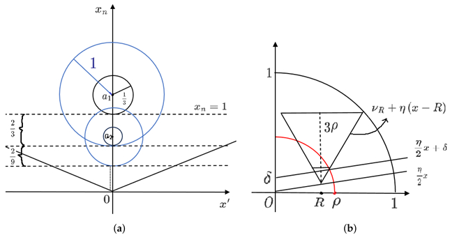
Let $ϵ=\frac{1}{3}$ and $r_2=\frac{6}{7}$ in Theorem 4. We take $a_i=\frac{4}{3}{\left(\frac{1}{3}\right)}^{i-1}$ and construct two series of balls and denote them as $\left\{B_{{\left(\frac{1}{3}\right)}^i}\left(0,a_i\right)\right\}$, $\left\{B_{{\left(\frac{1}{3}\right)}^{i-1}}\left(0,a_i\right)\right\}$ for all $i\in {\mathbb{N}}^{+}$, where $\left(0,a_i\right)$ represents a point in ${\mathbb{R}}^n$ with $x^{\prime }=0$ and $x_n=a_i$ (see figure(a)). In addition, we know that ${\displaystyle \sum _{i=1}^{\infty }\frac{2}{3^i}=1}$.

Obviously, $u\left(x\right)⩾1$ in $B_{\frac{1}{3}}\left(0,a_1\right)$ and by Theorem 4, we have $u\left(x\right)⩾{\left(\frac{1}{3}\right)}^q$ in $B_1\left(0,a_1\right)$. Thus, $u\left(x\right)⩾{\left(\frac{1}{3}\right)}^q$ in $B_{\frac{1}{3^2}}\left(0,a_2\right)$ and by Theorem 4 again, we have $u\left(x\right)⩾{\left(\frac{1}{3}\right)}^{2q}$ in $B_{\frac{1}{3}}\left(0,a_2\right)$. Repeating the above process, we have $u\left(x\right)⩾{\left(\frac{1}{3}\right)}^{\left(k+1\right)q}$ in $B_{\frac{1}{3^k}}\left(0,a_{k+1}\right)$, for all $k\in \mathbb{N}$.

For any $t\in \left(0,\frac{1}{3}\right)$, taking $k_0\in {\mathbb{N}}^{+}$, such that ${\displaystyle 1-2\sum _{i=1}^{k_0+1}{\left(\frac{1}{3}\right)}^i⩽t⩽1-2{\displaystyle \sum _{i=1}^{k_0}}{\left(\frac{1}{3}\right)}^i}$, then we have $t{e}_n\in B_{{\left(\frac{1}{3}\right)}^{k_0}}\left(0,a_{k_0+1}\right)$ and ${\left(\frac{1}{3}\right)}^{k_0+1}⩽t⩽{\left(\frac{1}{3}\right)}^{k_0}$. Hence, we have $u\left(t{e}_n\right)⩾{\left(\frac{1}{3}\right)}^{\left(k_0+1\right)q}$. Then $\frac{k_0+1}{k_0}\le 2$ implies

$${\left(\frac{1}{3}\right)}^{\left(k_0+1\right)q}⩾{\left[{\left(\frac{1}{3}\right)}^{k_0}\right]}^{2q}⩾t^{2q}.$$

Taking $q^{*}:=2q$, then we have

$$u\left(t{e}_n\right)⩾t^{2q}=t^{q^{*}},forallt\in \left(0,\frac{1}{3}\right).$$

Finally, if we take $\eta =\frac{1}{7\sqrt{n-1}}$, then all the balls will be located in cone ${\mathcal{C}}_{\eta }$. □

The following theorem shows that, by constructing an iteration, the solution of $\mathcal{L}u=f$ is positive at some distance from the boundary.

Theorem 7.

Let Ω be a Lipschitz domain with the Lipschitz constant $L<\frac{\eta }{2}$. The positive constants η and $q^{*}$ are determined by Lemma 1. Let u satisfy

$$\left\{\begin{array}{cc}\mathcal{L}u=f\hfill & in\Omega \cap B_1\hfill \\ u=0\hfill & on\partial \Omega \hfill \\ u\ge 1\hfill & in\Omega \cap \left\{x\in B_1:{\Gamma }_h\left(x\right)>\delta \right\}\hfill \\ u\ge -ϵ\hfill & in\Omega \cap B_1,\hfill \end{array}\right..$$

(3.2)

where ${∥f∥}_{L^{\infty }\left(B_r\left(y\right)\right)}\le c_0{r}^{q^{*}-1}$, for any $r\in \left(0,1\right)$, $y\in \partial \Omega \cap B_1$.

Then we have

$$\left\{\begin{array}{cc}u\ge {\rho }^{q^{*}+1}\hfill & in\Omega \cap \left\{x\in B_{\rho }:{\Gamma }_h\left(x\right)>\rho \delta \right\}\hfill \\ u\ge -{\rho }^{q^{*}+1}ϵ\hfill & in\Omega \cap B_{\rho },\hfill \end{array}\right.$$

(3.3)

for some small enough constants ρ, ϵ, δ, $c_0\in \left(0,1\right)$ depending on λ, Λ and the dimension n.

Proof. 

Now that, we prove the first inequality in (3.3). For any point $\left({x_0}^{\prime },x_{0n}\right)\in \left\{x\in B_{\rho }:\rho \delta <{\Gamma }_h\left(x\right)<\delta \right\}$, we write $\widetilde{x_0}:=\left(x_0^{\prime },\omega \left(x_0^{\prime }\right)\right)$ and the cone

$${\mathcal{C}}_{\rho ,\eta }:=\widetilde{x_0}+\rho {\mathcal{C}}_{\eta }=\left\{x\in {\mathbb{R}}^n:\eta \left|x^{\prime }-{x_0}^{\prime }\right|<x_n-\omega \left({x_0}^{\prime }\right)<3\rho \right\}$$

and the positive upper cone

$${\mathcal{C}}_{\rho ,\eta }^{+}:={\mathcal{C}}_{\rho ,\eta }\cap \left\{x_n>\omega \left({x_0}^{\prime }\right)+\rho \right\},$$

where ${\mathcal{C}}_{\eta }=\left\{x\in {\mathbb{R}}^n:\eta \left|x^{\prime }\right|<x_n<3\right\}$.

Let $\rho =3\delta$, $R\in \left[0,\rho \right]$, ${\nu }_R:=\frac{\eta }{2}R$ and $x_{\rho }=\frac{\rho }{\eta }+R$ (see Figure 2). We have

$$\frac{\eta }{2}{x}_{\rho }+\delta =\frac{\eta }{2}\left(\frac{\rho }{\eta }+R\right)+\frac{\rho }{3}=\frac{5}{6}\rho +{\nu }_R.$$

Obviously, ${\nu }_R+\rho >{\nu }_R+\frac{5}{6}\rho$ implies that $C_{\rho ,\eta }^{+}\subset \Omega \cap \left\{x\in B_1:{\Gamma }_h\left(x\right)>\delta \right\}$. Now we take $\delta$ small enough, then we have ${\mathcal{C}}_{\rho ,\eta }\subset \Omega \cap B_1$. Because $\left({x_0}^{\prime },x_{0n}\right)\in \left\{x\in B_{\rho }:\rho \delta <{\Gamma }_h\left(x\right)<\delta \right\}$, we have

$$\rho \delta <x_{0n}-\omega \left(x_0^{\prime }\right)<\delta andthen\frac{\rho }{3}<\frac{x_{0n}-\omega \left(x_0^{\prime }\right)}{\rho }<\frac{1}{3}.$$

We define

$$\tilde{u}\left(x\right):=u\left(\widetilde{x_0}+\rho x\right)+ϵand\Phi \left(x\right):=\mathcal{L}\tilde{u}\left(x\right)={\rho }^{2}f\left(\widetilde{x_0}+\rho x\right).$$

Let $\tilde{u}=u_1+u_2$ satisfy

$$\left\{\begin{array}{cc}\mathcal{L}{u}_1=0\hfill & in{\mathcal{C}}_{\eta }\hfill \\ u_1=\tilde{u}\hfill & on\partial {\mathcal{C}}_{\eta }\hfill \end{array}\right.and\left\{\begin{array}{cc}\mathcal{L}{u}_2=\Phi \hfill & in{\mathcal{C}}_{\eta }\hfill \\ u_2=0\hfill & on\partial {\mathcal{C}}_{\eta }.\hfill \end{array}\right.$$

By Theorem 3, we have

$$\begin{array}{cc}\hfill {∥u_2∥}_{L^{\infty }\left({\mathcal{C}}_{\eta }\right)}& ⩽C{∥\Phi ∥}_{L^n\left({\mathcal{C}}_{\eta }\right)}⩽C{\rho }^2{\left({\int }_{{\mathcal{C}}_{\eta }}{\left|f\left(\widetilde{x_0}+\rho x\right)\right|}^{n}dx\right)}^{\frac{1}{n}}\hfill \\ & =C\rho {\left({\int }_{{\mathcal{C}}_{\rho ,\eta }}{\left|f\left(y\right)\right|}^{n}dy\right)}^{\frac{1}{n}}⩽C^{\prime }\rho {∥f∥}_{L^{\infty }\left(B_{\rho }\left(\widetilde{x_0}\right)\right)}{\left|B_{\rho }\left(\widetilde{x_0}\right)\right|}^{\frac{1}{n}}\hfill \\ & ⩽C^{\prime }C\left(n\right)c_0{\rho }^{q^{*}+1}.\hfill \end{array}$$

On the other hand, we apply Lemma 1 to $u_1$ to result that $u_1\left(t{e}_n\right)\ge t^{q^{*}}$, for any $t\in (0,\frac{1}{3})$. We have

$$u\left(\left({x_0}^{\prime },\omega \left({x_0}^{\prime }\right)\right)+\rho t{e}_n\right)\ge t^{q^{*}}-C^{\prime }C\left(n\right)c_0{\rho }^{q^{*}+1}-ϵ,foranyt\in (0,\frac{1}{3}).$$

Therefore, let $\rho ⩽{\left(\frac{1}{3}\right)}^{q^{*}+1}$, $ϵ⩽{\left(\rho \right)}^{q^{*}+1}$, $c_0⩽\frac{1}{C^{\prime }C\left(n\right)}$, then

$$\begin{array}{cc}\hfill u\left(x_0\right)& ⩾u\left(\left({x_0}^{\prime },\omega \left({x_0}^{\prime }\right)\right)+\rho \frac{x_{0n}-\omega \left(x_0^{\prime }\right)}{\rho }{e}_n\right)\hfill \\ & ⩾{\left(\frac{x_{0n}-\omega \left(x_0^{\prime }\right)}{\rho }\right)}^{q^{*}}-C^{\prime }C\left(n\right)c_0{\rho }^{q^{*}+1}-ϵ\hfill \\ & ⩾{\left(\frac{\rho }{3}\right)}^{q^{*}}-C^{\prime }C\left(n\right)c_0{\rho }^{q^{*}+1}-{\left(\rho \right)}^{q^{*}+1}\hfill \\ & ⩾{\rho }^{q^{*}+1}.\hfill \end{array}$$

Next, we prove the second inequality in (3.3). Let $x_0\in B_{1-2\delta }$ and ${\Gamma }_h\left(x\right)⩽\delta$ (recalling $\delta =\rho /3$). We define $v\left(x\right):=\frac{{u\left(x\right)}^{-}}{ϵ}⩾0$. Extending v by 0 below $\partial \Omega$, then we have $\mathcal{L}v⩾-\frac{f^{+}}{ϵ}$ in $B_{2\delta }\left(x_0\right)$. Let ${\mathcal{C}}_z$ be the downwards cone with slope $\eta$ and vertex in $z:=\left(x_0^{\prime },\omega \left(x_0^{\prime }\right)\right)$. Then we have $v=0$ in ${\mathcal{C}}_z\cap B_{2\delta }\left(x_0\right)$ and $\left|{\mathcal{C}}_z\cap B_{2\delta }\left(x_0\right)\right|⩾C\left(\eta \right)\left|B_{2\delta }\left(x_0\right)\right|$. Taking $c_0$ small enough, we have

$$\begin{array}{cc}\hfill {\left({\int }_{B_{2\delta }\left(x_0\right)}{\left|\frac{f^{+}}{ϵ}\right|}^n\right)}^{\frac{1}{n}}& ⩽{\left({\int }_{B_{3\delta }\left(z\right)}{\left|\frac{f^{+}}{ϵ}\right|}^n\right)}^{\frac{1}{n}}⩽\frac{1}{ϵ}{∥f∥}_{L^n\left(B_{3\delta }\left(z\right)\right)}\hfill \\ \hfill & ⩽\frac{3\delta C\left(n\right)}{ϵ}{∥f∥}_{L^{\infty }\left(B_{3\delta }\left(z\right)\right)}⩽c_{0}C\left(n\right)\frac{{\left(3\delta \right)}^{q^{*}}}{ϵ}\hfill \\ \hfill & ⩽\xi \left(\eta \right),\hfill \end{array}$$

(3.4)

where $\xi \left(\eta \right)$ come from Theorem 5. By Theorem 5, we have $v⩽1-\gamma$ in $B_{\delta }\left(x_0\right)$.

Now we define $v_j\left(x\right):=\frac{v}{{\left(1-\gamma \right)}^j}\left(x\right)$ in $B_{\delta }\left(x_0\right)$ with $x_0\in B_{1-2j\delta }$ and ${\Gamma }_h\left(x_0\right)⩽\delta$. By mathematical induction, it is easy to show that $v⩽{\left(1-\gamma \right)}^j$ in $B_{1-2j\delta }$, i.e. $u⩾-{\left(1-\gamma \right)}^jϵ$ in $B_{1-2j\delta }$. We take $j_0\in {\mathbb{N}}^{+}$ satisfied $1-2\left(j_0+1\right)\delta ⩽\rho ⩽1-2j_0\delta$ (recalling $\rho =3\delta$). Hence, we have

$$\frac{1}{\frac{2}{3}{j}_0+\frac{5}{3}}⩽\rho ⩽\frac{1}{\frac{2}{3}{j}_0+1}.$$

We take $\rho$ small enough, such that

$${\left(1-\gamma \right)}^{j_0}⩽{\left(\frac{1}{\frac{2}{3}{j}_0+\frac{5}{3}}\right)}^{q^{*}+1},$$

then ${\left(1-\gamma \right)}^{j_0}⩽{\rho }^{q^{*}+1}$.

As same as (3.4), we have

$$\begin{array}{cc}\hfill {\left({\int }_{B_{2\delta }\left(x_0\right)}{\left|\frac{f^{+}}{{\left(1-\gamma \right)}^{j_0}ϵ}\right|}^n\right)}^{\frac{1}{n}}& ⩽\frac{1}{{\left(1-\gamma \right)}^{j_0}ϵ}{∥f∥}_{L^n\left(B_{3\delta }\left(z\right)\right)}\hfill \\ & ⩽c_{0}C\left(n\right)\frac{{\left(3\delta \right)}^{q^{*}}}{{\left(1-\gamma \right)}^{j_0}ϵ}\hfill \\ & ⩽\xi \left(\eta \right).\hfill \end{array}$$

By $1-2j_0\delta ⩾\rho$ with ${\left(1-\gamma \right)}^{j_0}⩽{\rho }^{q^{*}+1}$ and $u⩾-{\left(1-\gamma \right)}^{j_0}ϵ$ in $B_{1-2j_0\delta }$, then we have $u⩾-{\rho }^{q^{*}+1}ϵ$ in $B_{\rho }$. □

Now, we iterate Theorem 7 to obtain the following proposition.

Proposition 2.

Let Ω be a Lipschitz domain with the Lipschitz constant $L<\frac{\eta }{2}$. The positive constants η and $q^{*}$ are determined by Lemma 1. Let u be a weak solution of (3.2) with ${∥f∥}_{L^{\infty }\left(B_r\left(y\right)\right)}\le c_0{r}^{q^{*}-1}$, for any $r\in \left(0,1\right)$, $y\in \partial \Omega \cap B_1$.

Then we have

$$\left\{\begin{array}{cc}u>0\hfill & in\Omega \cap B_{2/3}\hfill \\ u\left(t{e}_n\right)⩾t^{q^{*}+1}\hfill & forallt\in \left(0,1\right).\hfill \end{array}\right.$$

Proof. 

Let $u_0\left(x\right):=u\left(x\right)$ and $f_0\left(x\right):=f\left(x\right)$. We define

$$u_{j+1}\left(x\right):=\frac{u_j\left(\rho x\right)}{{\rho }^{q^{*}+1}},f_{j+1}\left(x\right):=\frac{f_j\left(\rho x\right)}{{\rho }^{q^{*}-1}}.$$

where $x\in {\Omega }_{j+1}$ and $\rho x\in \rho {\Omega }_{j+1}:={\Omega }_j$. Obviously, $L_j\ge L_{j+1}$, where $L_j$ is the Lipschitz constant of ${\Omega }_j$.

First, we already have ${∥f_0∥}_{L^{\infty }\left(B_r\left(y\right)\right)}\le c_0{r}^{q^{*}-1}$, for any $r\in \left(0,1\right)$, $y\in \partial \Omega \cap B_1$. By mathematical induction, we have

$$\left\{\begin{array}{cc}\mathcal{L}{u}_j=f_j\hfill & in{\Omega }_j\cap B_1\hfill \\ u_j=0\hfill & on\partial {\Omega }_j\hfill \end{array}\right.with\left\{\begin{array}{cc}{u}_j\ge 1\hfill & in{\Omega }_j\cap \left\{x\in B_1:{\Gamma }_h\left(x\right)>\delta \right\}\hfill \\ u_j\ge -ϵ\hfill & in{\Omega }_j\cap B_1,\hfill \end{array}\right.$$

where ${∥f_j∥}_{L^{\infty }\left(B_r\left(y\right)\right)}\le c_0{r}^{q^{*}-1}$, for any $r\in \left(0,1\right)$, $y\in \partial \Omega \cap B_1$. By Theorem 7, we have

$$\left\{\begin{array}{cc}{u}_j\ge {\rho }^{q^{*}+1}\hfill & in{\Omega }_j\cap \left\{x\in B_{\rho }:{\Gamma }_h\left(x\right)>\rho \delta \right\}\hfill \\ u_j\ge -{\rho }^{q^{*}+1}ϵ\hfill & in{\Omega }_j\cap B_{\rho },\hfill \end{array}\right.$$

then

$$\left\{\begin{array}{cc}{u}_{j+1}\ge 1\hfill & in{\Omega }_{j+1}\cap \left\{x\in B_1:{\Gamma }_h\left(x\right)>\delta \right\}\hfill \\ u_{j+1}\ge -ϵ\hfill & in{\Omega }_{j+1}\cap B_1.\hfill \end{array}\right.$$

Moreover, we have

$$\begin{array}{cc}\hfill {∥f_{j+1}∥}_{L^{\infty }\left(B_r\left(y\right)\right)}& =\frac{1}{{\rho }^{q^{*}-1}}{∥f_j\left(\rho x\right)∥}_{L^{\infty }\left(B_r\left(y\right)\right)}\hfill \\ & ⩽\frac{c_0}{{\rho }^{q^{*}-1}}{\left(\rho r\right)}^{q^{*}-1}\hfill \\ & =c_0{r}^{q^{*}-1}.\hfill \end{array}$$

So for all $j\in \mathbb{N}$, we have $u_j\left(t{e}_n\right)⩾1$, for every $t\in \left(\delta ,1\right)$.

For any $t\in \left(0,1\right)$, there exists $j_0\in \mathbb{N}$ such that $\delta <\frac{t}{{\rho }^{j_0}}<1$. Thus, we have $t<{\rho }^{j_0}$ and

$$u\left(t{e}_n\right)=u_0\left(t{e}_n\right)={\rho }^{q^{*}+1}{u}_1\left(\frac{t{e}_n}{\rho }\right)=...={\rho }^{j_0\left(q^{*}+1\right)}{u}_{j_0}\left(\frac{t{e}_n}{{\rho }^{j_0}}\right)⩾t^{q^{*}+1}.$$

Finally, taking $ϵ$, $\rho$ and $c_0$ smaller, then $u\left(x_0+\frac{x}{3}\right)$ also satisfy (5) for any $x_0\in B_{2/3}\cap \partial \Omega$. By translating the coordinates, we get

$$u\left(x_0+t\frac{e_n}{3}\right)>0,forallt\in \left(0,1\right).$$

Then this implies

$$u>0in\Omega \cap B_{2/3}.$$

□

3.1. Proof of Theorem 1

Proof. 

Let $\Omega$ be a Lipschitz domain with the Lipschitz constant $L<\eta /2$. The positive constants $\eta$ and $q^{*}$ are determined by Lemma 1. By Theorem 6 and Proposition 1, we have $u⩽M$ in $B_{3/4}$. We consider v in the set $E:=\left\{x\in {\overline{B}}_{3/4}:{\Gamma }_h\left(x\right)⩾\left(3\delta \right)/4\right\}$. Obviously, $E\subset \left\{x\in {\overline{B}}_{1-\left(3\delta \right)/4}:{\Gamma }_h\left(x\right)⩾\left(3\delta \right)/4\right\}$. By Theorem 6 and $v\left(e_n/2\right)⩾1$, we have

$$v⩾C^{-1}-{∥f∥}_{L^n\left(B_1\right)}⩾C^{-1}-C\left(n\right){∥f∥}_{L^{\infty }\left(B_1\right)}⩾C^{-1}-C\left(n\right)c_0⩾{\left(2C\right)}^{-1}:=minE,$$

where the constant $c_0$ is small enough such that $C^{-1}-C\left(n\right)c_0⩾{\left(2C\right)}^{-1}$.

We define

$$\phi \left(x\right):=\frac{1+ϵ}{m}v\left(x\right)-\frac{ϵ}{M}u\left(x\right)$$

where $ϵ>0$ is chosen later. Once we prove that $\phi >0$ in $B_{1/2}$, by choosing $C=M\left(1+ϵ\right)/\left(mϵ\right)$, then $Cv-u>0$ follows.

Obviously, $\phi ⩾v/m⩾1$ in E, and $\phi ⩾-ϵ$ in $B_{3/4}$. We have

$$\begin{array}{cc}\hfill {∥\mathcal{L}\phi ∥}_{L^{\infty }\left(B_r\left(y\right)\right)}& ⩽\frac{1+ϵ}{m}{∥\mathcal{L}v∥}_{L^{\infty }\left(B_r\left(y\right)\right)}+\frac{ϵ}{M}{∥\mathcal{L}u∥}_{L^{\infty }\left(B_r\left(y\right)\right)}\hfill \\ & ⩽\left(\frac{1+ϵ}{m}+\frac{ϵ}{M}\right)c_0{r}^{q^{*}-1},foranyr\in \left(0,1\right),y\in \partial \Omega .\hfill \end{array}$$

Let $\tilde{\phi }\left(x\right):=\phi \left(3x/4\right)$. Then $\tilde{\phi }⩾1$ in $\Omega \cap \left\{x\in B_1:{\Gamma }_h\left(x\right)⩾\delta \right\}$ and $\tilde{\phi }⩾-ϵ$ in $\Omega \cap B_1$. Taking $ϵ$, $c_0>0$ small enough and applying Proposition 2, then we get $\tilde{\phi }>0$ in $B_{2/3}$. Thus, $\phi >0$ in $B_{1/2}$. □

4. Proof of Theorem 2

A simple lemma is given here to prepare for the following iteration of the ball in the Hölder cone.

Lemma 2.

Let constants $ϵ\in \left(0,1\right),\eta >0$ and $\alpha \in \left[\frac{1}{2},1\right]$. Then there exists a decreasing and positive sequence ${\left\{R_k\right\}}_{k=1}^{\infty }$ satisfied $R_k\to 0$ as $k\to +\infty$ and

$$ϵR_k^{\alpha }=1-\eta {\displaystyle \sum _{j=1}^k}{R}_j,$$

(4.1)

for any $k\in {\mathbb{N}}^{+}$. Moreover, there exists a constant $C_1>0$ such that

$$ϵR_k^{\frac{1}{2}}⩽\frac{C_1{ϵ}^2}{\eta k},foranyk\in {\mathbb{N}}^{+}.$$

(4.2)

Proof. 

We apply mathematical induction to prove (4.1). First, we show that there exists $R_1$ satisfying $ϵR_1^{\alpha }=1-\eta R_1$. Let $\phi \left(t\right):=1-\eta t-ϵt^{\alpha }$ and note that $\phi \left(0\right)=1>0$, $\phi \left(\frac{1}{\eta }\right)=-ϵ{\left(\frac{1}{\eta }\right)}^{\alpha }<0$ with ${\phi }^{\prime }\left(t\right)<0$ in $\left(0,\frac{1}{\eta }\right)$. By the zero point theorem, there exists $R_1$ such that $1-\eta R_1-ϵR_1^{\alpha }=0$. By mathematical induction, we suppose that $ϵR_k^{\alpha }=1-\eta {\displaystyle \sum _{j=1}^k}{R}_j$.

Next, we will show (4.1) for $k+1$. Denoting $a_k=1-\eta {\displaystyle \sum _{j=1}^{k-1}}{R}_j$, then we have ${\displaystyle 1-\eta \sum _{j=1}^k{R}_j=1-\eta \sum _{j=1}^{k-1}{R}_j-\eta R_k=a_k-\eta R_k}$. We define

$$\begin{array}{cc}\hfill \Phi \left(t\right)& :=a_k-\eta R_k-\eta t-ϵt^{\alpha }\hfill \\ & =ϵR_k^{\alpha }-ϵt^{\alpha }-\eta t.\hfill \end{array}$$

Then we have $\Phi \left(0\right)=ϵR_k^{\alpha }$ and $\Phi \left(R_k\right)=-\eta R_k^{\alpha }<0$ with ${\Phi }^{\prime }\left(t\right)<0$ in $\left(0,R_k\right)$. By the zero point theorem, there exists $R_{k+1}$ satisfied $0<R_{k+1}<R_k$ and $a_k-\eta R_k-\eta R_{k+1}-ϵR_{k+1}^{\alpha }=0$, i.e. $ϵR_{k+1}^{\alpha }=a_k-\eta \left(R_k+R_{k+1}\right)$.

We deserve that $0<R_{k+1}<R_k$ and

$$ϵR_k-ϵR_{k+1}=\eta R_{k+1}.$$

(4.3)

We have $R_{\infty }={lim}_{k\to \infty }{R}_k=0$. By (4.3) and letting $k\to \infty$, we have $R_{\infty }=0$. By (4.1), we get ${\displaystyle \eta \sum _{j=1}^{\infty }{R}_j=1}$.

Finally, we show (4.2). Obviously, if $\alpha =\frac{1}{2}$ holds true, then $\alpha \in [\frac{1}{2},1]$ holds even more. So, we consider $\alpha =\frac{1}{2}$. We have $ϵR_k^{\frac{1}{2}}-ϵR_{k+1}^{\frac{1}{2}}=\eta R_{k+1}$, i.e. $R_k^{\frac{1}{2}}-R_{k+1}^{\frac{1}{2}}=\frac{\eta }{ϵ}{R}_{k+1}:=C_0{R}_{k+1}$ with $C_0$ depending only on η and ϵ. Now, we have $R_k=R_{k+1}+2C_0{R}_{k+1}^{\frac{3}{2}}+C_0^2{R}_{k+1}^2$. For k large enough, we have $\left(R_k-R_{k+1}\right)/\left(2C_0{R}_{k+1}^{\frac{3}{2}}\right)=1+\frac{C_0}{2}{R}_{k+1}^{\frac{1}{2}}\to 1$. Hence, we get $R_k-R_{k+1}\backsim 2C_0{R}_{k+1}^{\frac{3}{2}}$ and

$$\begin{array}{cc}\hfill \underset{k\to \infty }{\lim }{k}^2{R}_k& =\underset{k\to \infty }{\lim }{k}^2/\left(1/R_k\right)\hfill \\ & =\underset{k\to \infty }{\lim }\left[{(k+1)}^2-k^2\right]/\left(1/R_{k+1}-1/R_k\right)\hfill \\ & =\underset{k\to \infty }{\lim }(2k+1)R_{k+1}^2/\left(2C_0{R}_{k+1}^{\frac{3}{2}}\right)\hfill \\ & =\underset{k\to \infty }{\lim }\left[(2k+1)-(2k-1)\right]/\left[2C_0(1/\sqrt{R_{k+1}}-1/\sqrt{R_k})\right]\hfill \\ & =\underset{k\to \infty }{\lim }\sqrt{R_k{R}_{k+1}}/\left[C_0(\sqrt{R_k}-\sqrt{R_{k+1}})\right]\hfill \\ & =\underset{k\to \infty }{\lim }{R}_{k+1}/\left(C_0^2{R}_{k+1}\right)\hfill \\ & =1/C_0^2.\hfill \end{array}$$

Hence, we have $R_k^{\frac{1}{2}}\backsim 1/\left(C_{0}k\right)=ϵ/\left(\eta k\right)$.

By $ϵR_k^{\frac{1}{2}}\backsim {ϵ}^2/\left(\eta k\right)$, there exists a constant $C_1$ such that $\left(C_1{ϵ}^2\right)/\left(\eta k\right)⩾ϵR_k^{\frac{1}{2}}$, for any $k\in {\mathbb{N}}^{+}$.

□

The following lemma is the decay lemma of the weak supersolution in the Hölder cone. This lemma plays a crucial role in the proof of the following theorem.

Lemma 3.

Let $\alpha \in \left[\frac{1}{2},1\right]$. There exist constants $C_2>0$ and $\eta >0$ depending on $\alpha ,\lambda ,\Lambda$ and the dimension n, such that the following holds.

Let u be a solution of

$$\left\{\begin{array}{cc}\mathcal{L}u\le 0\hfill & in{E}_{\eta }\hfill \\ u\ge 1\hfill & in\left\{x_n\ge 1\right\}\cap E_{\eta }\hfill \\ u\ge 0\hfill & on\partial E_{\eta },\hfill \end{array}\right.$$

(4.4)

where the $E_{\eta }=\left\{x\in {\mathbb{R}}^n:\frac{\eta }{2}{\left|x^{\prime }\right|}^{\alpha }<x_n<3\right\}$.

Then for any $t\in (0,\frac{1}{3})$, we have $u\left(t{e}_n\right)⩾e^{-\frac{C_2}{t}}$.

Proof. 

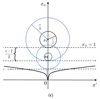
We take $R_1=\frac{1}{3}$ and $\eta =\left(1-\frac{e-1}{3}\right)3^{\alpha }$. By Lemma 2, we have a decreasing and positive sequence $\left\{R_k\right\}$ satisfied $R_k\to 0$ as $k\to +\infty$ and $\eta {R_k}^{\alpha }=1-(e-1){\displaystyle \sum _{j=1}^k}{R}_j$ for any $k\in {\mathbb{N}}^{+}$. Moreover, there exists a constant $C_1$ such that $\frac{C_1{ϵ}^2}{\eta k}⩾ϵR_k^{\frac{1}{2}}$, for any $k\in {\mathbb{N}}^{+}$.

We constructed two series of balls and denoted them as $\left\{B_{R_i}\left(0,a_i\right)\right\}$ and $\left\{B_{e{R}_i}\left(0,a_i\right)\right\}$, for all $i\in {\mathbb{N}}^{+}$ (see figure (c)). Now, there exists $k_0\in {\mathbb{N}}^{+}$ such that $1-(e-1){\displaystyle \sum _{j=1}^{k_0+1}}{R}_j⩽t⩽1-(e-1){\displaystyle \sum _{j=1}^{k_0}}{R}_j$, i.e. $\eta R_{k_0+1}^{\alpha }⩽t⩽\eta R_{k_0}^{\alpha }$ and $t{e}_n\in B_{2e{R}_{k_0+1}}\left(x_{k_0+1}\right)$.

As $u\left(x\right)⩾1$ in $B_{R_1}\left(x_1\right)$, Theorem 4 implies that $u\left(x\right)⩾e^{-q}$ in $B_{e{R}_1}\left(x_1\right)$. Hence, $u\left(\tau e^n\right)⩾e^{-q}$ in $B_{R_2}\left(x_2\right)$. By Theorem 4 again, we have $u\left(x\right)⩾e^{-2q}$ in $B_{2e{R}_2}\left(x_2\right)$. Now keep doing it this way, we get $u\left(x\right)⩾e^{-kq}$ in $B_{e{R}_k}\left(x_k\right)$ for any $k\in {\mathbb{N}}^{+}$. Hence, $u\left(t{e}^n\right)⩾e^{-(k_0+1)q}=e^{-q}{\left(e^{-q}\right)}^{k_0}$ and $\eta R_{k_0}^{\frac{1}{2}}⩽\frac{C_1{\eta }^2}{(e-1)k_0}$. As $\eta R_{k_0}^{\frac{1}{2}}⩾\eta R_{k_0}^{\alpha }⩾t$, we have $t⩽\frac{C_1{\eta }^2}{(e-1)k_0}$, i.e. $k_0⩽\frac{C_1{\eta }^2}{(e-1)t}$. Because $t<1$ and $q>1$, we have $e^{-q}{\left(e^{-q}\right)}^{k_0}⩾\left(e^{-q}\right){\left(e^{-q}\right)}^{\frac{C_1{\eta }^2}{(e-1)t}}⩾e^{-\frac{q{C}_1{\eta }^2+q}{t}}:=e^{-\frac{C_2}{t}}$ for any $t\in (0,\frac{1}{3})$. Thus, we have $u\left(t{e}_n\right)⩾e^{-\frac{C_2}{t}}$, for any $t\in (0,\frac{1}{3})$.

□

The following theorem works similarly to Theorem 7.

Theorem 8.

Let Ω be a Hölder domain with $\alpha \in [1/2,1)$ and the Hölder constant $H<\frac{4-e}{4\sqrt{3}}$. Let u satisfy

$$\left\{\begin{array}{cc}\mathcal{L}u=f\hfill & in\Omega \cap B_1\hfill \\ u=0\hfill & on\partial \Omega \hfill \\ u\ge 1\hfill & in\Omega \cap \left\{x\in B_1:{\Gamma }_h\left(x\right)>\delta \right\}\hfill \\ u\ge -ϵ\hfill & in\Omega \cap B_1,\hfill \end{array}\right.$$

(4.5)

. ${∥f∥}_{L^{\infty }\left(B_r\left(y\right)\right)}\le c_0{r}^{-2}exp\left(-4C_2{r}^{-1}\right)$ for any $r\in \left(0,1/2\right)$, $y\in \partial \Omega \cap B_1$.Then we have

$$\left\{\begin{array}{cc}u\ge exp\left(-4C_2{\rho }^{-1}\right)\hfill & in\Omega \cap \left\{x\in B_{\rho }:{\Gamma }_h\left(x\right)>\rho \delta \right\}\hfill \\ u\ge -exp\left(-4C_2{\rho }^{-1}\right)ϵ\hfill & in\Omega \cap B_{\rho },\hfill \end{array}\right.$$

(4.6)

where the positive constant $C_2$ is determined by Lemma 3 and some small enough constants ρ, ϵ, δ, $c_0\in \left(0,1\right)$ depend on $\alpha ,\lambda$, Λ and the dimension n.

Proof. 

Now that, we prove the first inequality in (4.6). For any $\left({x_0}^{\prime },x_{0n}\right)\in \left\{x\in B_{\rho }:\rho \delta <{\Gamma }_h\left(x\right)<\delta \right\}$, we write $\widetilde{x_0}:=\left(x_0^{\prime },\omega \left(x_0^{\prime }\right)\right)$ and the Hölder cone

$$E_{\rho ,\eta }=\widetilde{x_0}+\rho E_{\eta }=\left\{x\in {\mathbb{R}}^n:\frac{\eta }{2}{\left|x^{\prime }-{x_0}^{\prime }\right|}^{\alpha }<x_n-\omega \left({x_0}^{\prime }\right)<3\rho \right\}$$

and the positive upper Hölder cone

$$E_{\rho }^{+}=E_{\rho ,\eta }\cap \left\{x_n>\omega \left({x_0}^{\prime }\right)+\rho \right\},$$

where $E_{\eta }=\left\{x\in {\mathbb{R}}^n:\frac{\eta }{2}{\left|x^{\prime }\right|}^{\alpha }<x_n<3\right\}$.

We take $\rho =3\delta$, it’s easy to get $E_{\rho }^{+}\subset \Omega \cap \left\{x\in B_1:{\Gamma }_h\left(x\right)>\delta \right\}$. If $\delta$ small enough, we have $E_{\rho ,\eta }\subset \Omega \cap B_1$. Because $x_0=\left({x_0}^{\prime },x_{0n}\right)$ in $\left\{x\in B_{\rho }:\rho \delta <{\Gamma }_h\left(x\right)<\delta \right\}$, we have

$$\rho \delta <x_{0n}-\omega \left(x_0^{\prime }\right)<\delta andthen\frac{\rho }{3}<\frac{x_{0n}-\omega \left(x_0^{\prime }\right)}{\rho }<\frac{1}{3}.$$

We define

$$\tilde{u}\left(x\right):=u\left(\widetilde{x_0}+\rho x\right)+ϵand\Phi \left(x\right):=\mathcal{L}\tilde{u}\left(x\right)={\rho }^{2}f\left(\widetilde{x_0}+\rho x\right).$$

Let $\tilde{u}=u_1+u_2$ satisfy

$$\left\{\begin{array}{cc}\mathcal{L}{u}_1=0\hfill & in{E}_{\eta }\hfill \\ u_1=\tilde{u}\hfill & on\partial E_{\eta }\hfill \end{array}\right.and\left\{\begin{array}{cc}\mathcal{L}{u}_2=\Phi \hfill & in{E}_{\eta }\hfill \\ u_2=0\hfill & on\partial E_{\eta }.\hfill \end{array}\right.$$

By Theorem 3, we have

$$\begin{array}{cc}\hfill {∥u_2∥}_{L^{\infty }\left(E_{\eta }\right)}& ⩽C{∥\Phi ∥}_{L^n\left(E_{\eta }\right)}⩽C{\rho }^2{\left({\int }_{E_{\eta }}{\left|f\left(\widetilde{x_0}+\rho x\right)\right|}^{n}dx\right)}^{\frac{1}{n}}\hfill \\ & =C\rho {\left({\int }_{E_{\rho ,\eta }}{\left|f\left(y\right)\right|}^{n}dy\right)}^{\frac{1}{n}}⩽C^{\prime }\rho {∥f∥}_{L^{\infty }\left(B_{\rho }\left(\widetilde{x_0}\right)\right)}{\left|B_{\rho }\left(\widetilde{x_0}\right)\right|}^{\frac{1}{n}}\hfill \\ & ⩽C^{\prime }C\left(n\right)c_{0}exp\left(-4C_2{\rho }^{-1}\right).\hfill \end{array}$$

On the other hand, we apply Lemma 3 to $u_1$ to result that $u_1\left(t{e}_n\right)\ge exp\left(-C_2{t}^{-1}\right)$, for any $t\in (0,\frac{1}{3})$. Then we get

$$u\left(\left({x_0}^{\prime },\omega \left({x_0}^{\prime }\right)\right)+\rho t{e}_n\right)\ge exp\left(-C_2{t}^{-1}\right)-C^{\prime }C\left(n\right)c_{0}exp\left(-4C_2{\rho }^{-1}\right)-ϵ,foranyt\in (0,\frac{1}{3}).$$

Therefore,

$$\begin{array}{cc}\hfill u\left(x_0\right)& ⩾u\left(\left({x_0}^{\prime },\omega \left({x_0}^{\prime }\right)\right)+\rho \frac{x_{0n}-\omega \left(x_0^{\prime }\right)}{\rho }{e}_n\right)\hfill \\ & ⩾exp\left(-C_2{\left(\frac{x_{0n}-\omega \left(x_0^{\prime }\right)}{\rho }\right)}^{-1}\right)-C^{\prime }C\left(n\right)c_{0}exp\left(-4C_2{\rho }^{-1}\right)-ϵ\hfill \\ & ⩾exp\left(-C_2{\left(\frac{\rho }{3}\right)}^{-1}\right)-C^{\prime }C\left(n\right)c_{0}exp\left(-4C_2{\rho }^{-1}\right)-ϵ\hfill \\ & ⩾3exp\left(-4C_2{\rho }^{-1}\right)-C^{\prime }C\left(n\right)c_{0}exp\left(-4C_2{\rho }^{-1}\right)-ϵ\hfill \\ & ⩾exp\left(-4C_2{\rho }^{-1}\right).\hfill \end{array}$$

Next, we prove the second inequality in (4.6). Let $x_0\in B_{1-2\delta }$ and ${\Gamma }_h\left(x\right)⩽\delta$. We define $v\left(x\right):=\frac{{u\left(x\right)}^{-}}{ϵ}⩾0$ and extend v by 0 below $\partial \Omega$. Thus, $\mathcal{L}v⩾-\frac{f^{+}}{ϵ}$ in $B_{2\delta }\left(x_0\right)$. We write $z:=\left(x_0^{\prime },\omega \left(x_0^{\prime }\right)\right)$. Let $E_z$ be the downwards Hölder cone with the Hölder constant $\eta$ and vertex in z. Then we have $v=0$ in $E_z\cap B_{2\delta }\left(x_0\right)$ and $\left|E_z\cap B_{2\delta }\left(x_0\right)\right|⩾C\left(\eta \right)\left|B_{2\delta }\left(x_0\right)\right|$. Hence, we have

$$\begin{array}{cc}\hfill {\left({\int }_{B_{2\delta }\left(x_0\right)}{\left|\frac{f^{+}}{ϵ}\right|}^n\right)}^{\frac{1}{n}}& ⩽{\left({\int }_{B_{3\delta }\left(z\right)}{\left|\frac{f^{+}}{ϵ}\right|}^n\right)}^{\frac{1}{n}}\hfill \\ & ⩽\frac{3\delta C\left(n\right)}{ϵ}{∥f∥}_{L^{\infty }\left(B_{3\delta }\left(z\right)\right)}\hfill \\ & ⩽c_{0}C\left(n\right)\frac{{\rho }^{-2}exp\left(-4C_2{\rho }^{-1}\right)}{ϵ}\hfill \\ & ⩽\xi \left(\eta \right),\hfill \end{array}$$

where $\xi \left(\eta \right)$ come from Theorem 5 and make $c_0$ small enough such that the last inequality holds. By Theorem 5, we have $v⩽1-\gamma$ in $B_{\delta }\left(x_0\right)$.

Now we define $v_j\left(x\right):=\frac{v}{{\left(1-\gamma \right)}^j}\left(x\right)$ in $B_{\delta }\left(x_0\right)$ with $x_0\in B_{1-2j\delta }$ and ${\Gamma }_h\left(x_0\right)⩽\delta$. By mathematical induction, it is easy to show that $v⩽{\left(1-\gamma \right)}^j$ in $B_{1-2j\delta }$, i.e. $u⩾-{\left(1-\gamma \right)}^jϵ$ in $B_{1-2j\delta }$. We take $j_0\in {\mathbb{N}}^{+}$ satisfied $1-2\left(j_0+1\right)\delta ⩽\rho ⩽1-2j_0\delta$, with $\rho =3\delta$. Hence, we have

$$\frac{1}{\frac{2}{3}{j}_0+\frac{5}{3}}⩽\rho ⩽\frac{1}{\frac{2}{3}{j}_0+1}.$$

We take $\rho$ small enough, such that

$$exp\left(j_{0}ln\left(1-\gamma \right)\right)⩽exp\left(-4C_2\left(\frac{2}{3}{j}_0+\frac{5}{3}\right)\right)andthen{\left(1-\gamma \right)}^{j_0}⩽exp\left(-4C_2\left(\frac{2}{3}{j}_0+\frac{5}{3}\right)\right).$$

Hence, we have ${\left(1-\gamma \right)}^{j_0}⩽exp\left(-4C_2{\rho }^{-1}\right)$.

Finally, we have

$$\begin{array}{cc}\hfill {\left({\int }_{B_{2\delta }\left(x_0\right)}{\left|\frac{f^{+}}{{\left(1-\gamma \right)}^{j_0}ϵ}\right|}^n\right)}^{\frac{1}{n}}& ⩽{\left({\int }_{B_{3\delta }\left(z\right)}{\left|\frac{f^{+}}{{\left(1-\gamma \right)}^{j_0}ϵ}\right|}^n\right)}^{\frac{1}{n}}⩽\frac{1}{{\left(1-\gamma \right)}^{j_0}ϵ}{∥f∥}_{L^n\left(B_{3\delta }\left(z\right)\right)}\hfill \\ & ⩽\frac{3\delta C\left(n\right)}{{\left(1-\gamma \right)}^{j_0}ϵ}{∥f∥}_{L^{\infty }\left(B_{3\delta }\left(z\right)\right)}⩽c_{0}C\left(n\right)\frac{{\rho }^{-2}exp\left(-4C_2{\rho }^{-1}\right)}{{\left(1-\gamma \right)}^{j_0}ϵ}\hfill \\ & ⩽\xi \left(\eta \right),\hfill \end{array}$$

where $\xi \left(\eta \right)$ come from Theorem 5 and make $c_0$ small enough such that the last inequality holds.

By $1-2j_0\delta ⩾\rho$ with ${\left(1-\gamma \right)}^{j_0}⩽exp\left(-4C_2{\rho }^{-1}\right)$, and $u⩾-{\left(1-\gamma \right)}^{j_0}ϵ$ in $B_{1-2j_0\delta }$.

Hence, we have $u⩾-exp\left(-4C_2{\rho }^{-1}\right)ϵ$ in $B_{\rho }$. □

Now, by iterating Theorem 8, we get the following proposition.

Proposition 3.

Let Ω be a Hölder domain with $\alpha \in [1/2,1)$ and the Hölder constant $H<\frac{4-e}{4\sqrt{3}}$. The positive constant $C_2$ is determined by Lemma 3. Let u be a weak solution of (4.5) and ${∥f∥}_{L^{\infty }\left(B_r\left(y\right)\right)}\le c_0{r}^{-2}exp\left(-4C_2{r}^{-1}\right)$, for any $r\in \left(0,1/2\right)$, $y\in \partial \Omega \cap B_1$.

Then we have

$$\left\{\begin{array}{cc}u>0\hfill & in\Omega \cap B_{2/3}\hfill \\ u\left(t{e}_n\right)⩾exp\left(-4C_2{t}^{-1}\right)\hfill & forallt\in \left(0,1\right).\hfill \end{array}\right.$$

Proof. 

Let $u_0\left(x\right):=u\left(x\right)$ and $f_0\left(x\right):=f\left(x\right)$. We define

$$u_{j+1}\left(x\right):=\frac{u_j\left(\rho x\right)}{exp\left(-4C_2{\rho }^{-1}\right)},f_{j+1}\left(x\right):=\frac{{\rho }^2{f}_j\left(\rho x\right)}{exp\left(-4C_2{\rho }^{-1}\right)}$$

with $x\in {\Omega }_{j+1}$ and $\rho x\in \rho {\Omega }_{j+1}:={\Omega }_j$, where the Hölder constant of ${\Omega }_{j+1}$ is the same as or smaller than ${\Omega }_j$.

First we already have ${∥f_0∥}_{L^{\infty }\left(B_r\left(y\right)\right)}\le c_0{r}^{-2}exp\left(-4C_2{r}^{-1}\right)$, for any $r\in \left(0,1/2\right)$, $y\in \partial \Omega \cap B_1$. By mathematical induction, we have

$$\left\{\begin{array}{cc}\mathcal{L}{u}_j=f_j\hfill & in{\Omega }_j\cap B_1\hfill \\ u_j=0\hfill & on\partial {\Omega }_j\hfill \end{array}\right.with\left\{\begin{array}{cc}{u}_j\ge 1\hfill & in{\Omega }_j\cap \left\{x\in B_1:{\Gamma }_h\left(x\right)>\delta \right\}\hfill \\ u_j\ge -ϵ\hfill & in{\Omega }_j\cap B_1,\hfill \end{array}\right.$$

where ${∥f_j∥}_{L^{\infty }\left(B_r\left(y\right)\right)}\le c_0{r}^{-2}exp\left(-4C_2{r}^{-1}\right)$, for any $r\in \left(0,1/2\right)$, $y\in \partial \Omega \cap B_1$. By Theorem 8, we have

$$\left\{\begin{array}{cc}{u}_j\ge exp\left(-4C_2{\rho }^{-1}\right)\hfill & in{\Omega }_j\cap \left\{x\in B_{\rho }:{\Gamma }_h\left(x\right)>\rho \delta \right\}\hfill \\ u_j\ge -exp\left(-4C_2{\rho }^{-1}\right)ϵ\hfill & in{\Omega }_j\cap B_{\rho }.\hfill \end{array}\right.$$

So, we have

$$\left\{\begin{array}{cc}{u}_{j+1}\ge 1\hfill & in{\Omega }_{j+1}\cap \left\{x\in B_1:{\Gamma }_h\left(x\right)>\delta \right\}\hfill \\ u_{j+1}\ge -ϵ\hfill & in{\Omega }_{j+1}\cap B_1.\hfill \end{array}\right.$$

Moreover, we have

$$\begin{array}{cc}\hfill {∥f_{j+1}∥}_{L^{\infty }\left(B_r\left(y\right)\right)}& =\frac{{\rho }^2}{exp\left(-4C_2{\rho }^{-1}\right)}{∥f_j\left(\rho x\right)∥}_{L^{\infty }\left(B_r\left(y\right)\right)}\hfill \\ & ⩽\frac{c_0{\rho }^2}{exp\left(-4C_2{\rho }^{-1}\right)}{\left(\rho r\right)}^{-2}exp\left(-4C_2{\left(\rho r\right)}^{-1}\right)\hfill \\ & ⩽c_0{r}^{-2}exp\left(-4C_2{r}^{-1}\right).\hfill \end{array}$$

Then for every $j\in \mathbb{N}$, we have $u_j\left(t{e}_n\right)⩾1$, for any $t\in \left(\delta ,1\right)$. For any $t\in \left(0,1\right)$, there exists $j_0\in \mathbb{N}$ such that $\delta <\frac{t}{{\rho }^{j_0}}<1$. Thus, $t<{\rho }^{j_0}<\frac{\rho }{j_0}$ and

$$u\left(t{e}_n\right)=u_0\left(t{e}_n\right)=exp\left(-4C_2{\rho }^{-1}\right)u_1\left(\frac{t{e}_n}{\rho }\right)=...=exp\left(-4j_0{C}_2{\rho }^{-1}\right)u_{j_0}\left(\frac{t{e}_n}{{\rho }^{j_0}}\right)⩾exp\left(-4C_2{t}^{-1}\right).$$

Finally, taking $ϵ$, $\delta$ and $c_0$ smaller, then $u\left(x_0+\frac{x}{3}\right)$ also satisfy (4.5) for any $x_0\in B_{2/3}\cap \partial \Omega$. By translating the coordinates, we get

$$u\left(x_0+t\frac{e_n}{3}\right)>0,forallt\in \left(0,1\right).$$

Then this implies

$$u>0in\Omega \cap B_{2/3}.$$

□

4.1. Proof of Theorem 2

Proof. 

By Theorem 6 and Proposition 1, we have $u⩽M$ in $B_{3/4}$. We consider the function v in the set $E:=\left\{x\in {\overline{B}}_{3/4}:{\Gamma }_h\left(x\right)⩾\left(3\delta \right)/4\right\}$. Obviously, $E\subset \left\{x\in {\overline{B}}_{1-\left(3\delta \right)/4}:{\Gamma }_h\left(x\right)⩾\left(3\delta \right)/4\right\}$. Thus, by Theorem 6 and $v\left(e_n/2\right)⩾1$, we have

$$v⩾C^{-1}-{∥f∥}_{L^n\left(B_1\right)}⩾C^{-1}-C\left(n\right){∥f∥}_{L^{\infty }\left(B_1\right)}⩾C^{-1}-C\left(n\right)c_0⩾{\left(2C\right)}^{-1}:=minE,$$

where the constant $c_0$ is small enough such that $C^{-1}-C\left(n\right)c_0⩾{\left(2C\right)}^{-1}$.

We define

$$\phi \left(x\right):=\frac{1+ϵ}{m}v\left(x\right)-\frac{ϵ}{M}u\left(x\right),$$

where $ϵ>0$ to be chosen later. We will prove that $\phi >0$ in $B_{1/2}$ and therefore, choosing $C=M\left(1+ϵ\right)/\left(mϵ\right)$, we have $Cv-u>0$.

Obviously, $\phi ⩾v/m⩾1$ in E, and $\phi ⩾-ϵ$ in $B_{3/4}$. We have

$$\begin{array}{cc}\hfill {∥\mathcal{L}\phi ∥}_{L^{\infty }\left(B_r\left(y\right)\right)}& ⩽\frac{1+ϵ}{m}{∥\mathcal{L}v∥}_{L^{\infty }\left(B_r\left(y\right)\right)}+\frac{ϵ}{M}{∥\mathcal{L}u∥}_{L^{\infty }\left(B_r\left(y\right)\right)}\hfill \\ & ⩽\left(\frac{1+ϵ}{m}+\frac{ϵ}{M}\right)c_0{r}^{-2}exp\left(-4C_2{r}^{-1}\right),foranyr\in \left(0,1/2\right),y\in \partial \Omega .\hfill \end{array}$$

Where the positive constant $C_2$ is determined by Lemma 3.

Let $\tilde{\phi }\left(x\right):=\phi \left(3x/4\right)$. Then $\tilde{\phi }⩾1$ in $\Omega \cap \left\{x\in B_1:{\Gamma }_h\left(x\right)⩾\delta \right\}$ and $\tilde{\phi }⩾-ϵ$ in $\Omega \cap B_1$. Taking small enough $ϵ$, $c_0>0$ to apply Proposition 3. We get $\tilde{\phi }>0$ in $B_{2/3}$, thus $\phi >0$ in $B_{1/2}$. □

References

- Allen, M.; Shahgholian, H. A new boundary Harnack principle (equations with right hand side). Arch. Ration. Mech. Anal 2019, 234, 1413–1444. [Google Scholar] [CrossRef]
- Ancona, A. Principe de Harnack a la frontiere et theoreme de Fatou pour un operateur elliptique dons un domaine lipschitzien. Ann. Inst 1978, Fourier 28, 169–213. [Google Scholar]
- Banuelos, R.; Bass, R.F.; Burdzy, K. Hölder domains and the boundary Harnack principle. Duke Math. J 1991, 64, 195–200. [Google Scholar] [CrossRef]
- Bass, R.F.; Burdzy, K. A boundary Harnack principle in twisted Hölder domains. Ann. Math 1991, 134, 253–276. [Google Scholar] [CrossRef]
- Bass, R.F.; Burdzy, K. Further regularity for the Signorini problem. J. Lond. Math. Soc 1994, 50, 157–169. [Google Scholar] [CrossRef]
- Caffarelli, L.A. Further regularity for the Signorini problem. Commun. Partial Differ. Equ 1979, 4, 1067–1075. [Google Scholar] [CrossRef]
- Caffarelli, L.A.; Fabes, E.; Mortola, S.; Salsa, S. Boundary behavior of non-negative solutions of elliptic operators in divergence form. Indiana Univ. Math. J 1981, 49, 621–640. [Google Scholar] [CrossRef]
- Caffarelli, L.A.; Crandall, M.; Kocan, A.; Swiech. On viscosity solutions of fully nonlinear equations with measurable ingredients. Commun. Pure Appl. Math 1996, 49, 365–398. [Google Scholar] [CrossRef]
- Caffarelli, L.A.; Cabré, X. The boundary Harnack principle for non-divergence form elliptic operators. Amer. Math. Soc. Colloq. Publ 1995, 43, 1067–1075. [Google Scholar]
- Dahlberg, B. On estimates of harmonic measure. Arch. Ration. Mech. Anal 1977, 65, 272–288. [Google Scholar] [CrossRef]
- De Giorgi, E. Sulla differenziabilità e l’analiticità delle estremali degli integrali multipli regolari (Italian). Mem. Accad. Sci. Torino, Cl. Sci. Fis. Mat. Nat 1957, 3, 25–43. [Google Scholar]
- De Silva, D.; Savin, O. Boundary Harnack estimates in slit domains and applications to thin free boundary problems. Rev. Mat. Iberoam 2016, 32, 891–912. [Google Scholar] [CrossRef]
- De Silva, D.; Savin, O. A short proof of boundary Harnack inequality. C J. Differ. Equ 2020, 269, 2419–2429. [Google Scholar] [CrossRef]
- De Silva, D.; Savin, O. On the boundary Harnack principle in Hölder domains. Mathematics in Engineering 2022, 4, 1–12. [Google Scholar] [CrossRef]
- DiBenedetto, E. Partial Differential Equations: Second Edition. Birkhäuser Basel, 2010. [Google Scholar]
- DiBenedetto, E. Some properties of De Giorgi classes. Rend. Istit. Mat. Univ. Trieste 2016, 48, 245–260. [Google Scholar]
- DiBenedetto, E.; Trudinger, N. Harnack inequalities for quasiminima of variational integrals. Ann. Inst. H. Poincaré Anal 1984, 1, 295–308. [Google Scholar]
- Fabes, E.; Garofalo, N.; Marin-Malave, S.; Salsa, S. Fatou theorems for some nonlinear elliptic equions. Rev. Mat. Iberoam 1988, 4, 227–252. [Google Scholar] [CrossRef]
- Ferrari, F. On Boundary Behavior of Harmonic Functions in Hölder Domains. J. Fourier. Anal. Appl 1998, 4, 447–461. [Google Scholar] [CrossRef]
- Giaquinta, M.; Giusti, E. On the regularity of the minima of variational integrals. Acta Math 1982, 148, 31–46. [Google Scholar] [CrossRef]
- Giaquinta, M.; Giusti, E. Quasiminima. Ann. Inst. H. Poincaré Anal.Non Linéaire 1984, 1, 79–107. [Google Scholar] [CrossRef]
- Gilbarg, D.; Trudinger, N.S. Elliptic Partial Differential Equations of Second Order, 1st ed.Fundamental Principles of Mathematical Sciences, 1998. [Google Scholar]
- Jerison, D.S.; Kenig, C.E. Boundary behavior of harmonic functions in non-tangentially accessible domains. Adv. Math 1982, 42, 80–147. [Google Scholar] [CrossRef]
- Kemper, J.T. A boundary Harnack principle for Lipschitz domains and the principle of positive singularities. Commun. Pure Appl. Math 1972, 25, 247–255. [Google Scholar] [CrossRef]
- Kim, H.; Safonov, M.V. Boundary Harnack principle for second order elliptic equations with unbounded drift. Problems in mathematical analysis. No. 61. J. Math. Sci. 2011, 1, 127–143. [Google Scholar] [CrossRef]
- Koike, S.; Swiech, A. Weak Harnack inequality for fully nonlinear uniformly elliptic PDE with unbounded ingredients. J. Math. Soc. Jpn 2009, 61, 723–755. [Google Scholar] [CrossRef]
- Koike, S. Local maximum principle for Lp-viscosity solutions of fully nonlinear elliptic PDEs with unbounded coefficients. Commun. Pure Appl. Anal 2012, 11, 1897–1910. [Google Scholar] [CrossRef]
- Krylov, N.V.; Safonov, M.V. An estimate for the probability of a diffusion process hitting a set of positive measure (Russian). Dokl. Akad. Nauk SSSR 1979, 1, 18–30. [Google Scholar]
- Ladyzhenskaya, O.A.; Ural’tseva, N. Linear and quasilinear elliptic equations. Academic Press: New York-London, 1968. [Google Scholar]
- Lian, Y.; Zhang, K. Boundary Lipschitz regularity and the Hopf lemma for fully nonlinear elliptic equations. arXiv 2018. [Google Scholar] [CrossRef]
- Ros-Oton, X.; Torres-Latorre, D. New boundary Harnack inequalities with right hand side. J. Differ Equations 2021, 288, 204–249. [Google Scholar] [CrossRef]
- Sirakov, B. Boundary Harnack estimates and quantitative strong maximum principles for uniformly elliptic PDE. Int. Math. Res. Not. IMRN 2017, 2018, 7457–7482. [Google Scholar] [CrossRef]
- Sirakov, B. Global integrability and boundary estimates for uniformly elliptic PDE in divergence form. arXiv 2019. [Google Scholar] [CrossRef]
- Trudinger, N.S. Local estimates for subsolutions and supersolutions of general second order elliptic quasilinear equations. Invent. Math. 1980, 61, 67–79. [Google Scholar] [CrossRef]
Disclaimer/Publisher’s Note: The statements, opinions and data contained in all publications are solely those of the individual author(s) and contributor(s) and not of MDPI and/or the editor(s). MDPI and/or the editor(s) disclaim responsibility for any injury to people or property resulting from any ideas, methods, instructions or products referred to in the content. |
© 2025 by the authors. Licensee MDPI, Basel, Switzerland. This article is an open access article distributed under the terms and conditions of the Creative Commons Attribution (CC BY) license (http://creativecommons.org/licenses/by/4.0/).
Copyright: This open access article is published under a Creative Commons CC BY 4.0 license, which permit the free download, distribution, and reuse, provided that the author and preprint are cited in any reuse.