
Submitted:
31 May 2025
Posted:
04 June 2025
You are already at the latest version
Abstract
Gravitational wave detection remains challenging due to low signal amplitudes often obscured by instrumental noise, particularly in low signal-to-noise ratio scenarios where conventional Convolutional Neural Networks (CNNs) exhibit limited effectiveness due to their restricted receptive fields. This paper presents an enhanced EfficientNet-based architecture for continuous gravitational wave classification that addresses these limitations through several key innovations. We transform input data into spectrograms using constant Q transformation and augment the baseline EfficientNet architecture with an additional convolutional layer featuring enlarged kernel sizes to expand the receptive field. This modification enables improved detection of weak gravitational wave signals embedded in noisy datasets while enhancing texture feature learning capabilities. Through K-fold cross-validation on a private dataset, our proposed model achieves Area Under the Curve (AUC) scores ranging from 0.878 to 0.978, demonstrating significantly enhanced sensitivity to gravitational wave signals. These results indicate substantial potential for advancing next-generation detection methodologies in astrophysical applications and improving the reliability of gravitational wave detection systems.
Keywords:
gravitational wave detection
; EfficientNet
; Convolutional Neural Networks
; signal-to-noise ratio
; constant Q transformation
; spectrogram analysis
; deep learning
1. Introduction
Gravitational waves resulting from binary mergers are now being routinely detected by the advanced LIGO and Virgo observatories [4,20]. In contrast, the detection of much weaker and longer-lasting narrow-band continuous gravitational waves (CW) emitted by spinning, deformed neutron stars remains elusive, despite numerous search efforts over the past decade and ongoing enhancements in detection methodologies [7]. In recent years, an increasing number of strategies for detecting CW have emerged; however, these approaches often require substantial computational resources [8]. Concurrently, the low signal-to-noise ratio (SNR) associated with attractive force wave signals presents challenges for traditional detection methods. Typically, researchers have sought to enhance the SNR by aggregating larger datasets to address this issue. However, the application of deep learning algorithms offers a more effective alternative. In recent years, the availability of substantial computational resources, such as graphics processing units (GPUs), has facilitated the adoption of deep learning techniques, particularly convolutional neural networks, in this domain [9,12]. Nevertheless, in the context of perfectly coherent matched filtered searches, the associated computational expense escalates with the high power, approximately represented as , where T denotes the duration of the data time span and n is typically greater than or equal to 5. This phenomenon generally constrains the maximum coherence duration to a range of several days to a few weeks, beyond which the computational demands become impractical [8]. In recent years, the emergence of various architectures of Convolutional Neural Networks (CNNs) has prompted investigations into their applicability for detecting continuous wave (CW) signals associated with attractive force waves. Numerous studies have examined the potential of Deep Neural Networks (DNNs) to enhance CW searches, particularly as a method for clustering and following up on search candidates, thereby reducing the computational burden associated with follow-up analyses. Additionally, DNNs have been employed to alleviate the impact of instrumental noise artifacts. Evidence suggests that DNNs can also expedite the search process for long-duration transient CW signals. By leveraging CNNs, it is possible to transfer the computationally intensive components of traditional methodologies to the preparatory phase of the search, which includes architecture optimization and the training of the network to determine optimal weights. Consequently, the execution time for processing a given input vector is significantly reduced, typically to mere fractions of a second. Furthermore, accurately determining the noise distribution—essential for estimating the false alarm rate (pfa)—and establishing the upper limits of measurement necessitates conducting multiple repeated searches across various input datasets, both with and without the inclusion of injected signals. Consequently, the comparative advantage in search speed offered by Convolutional Neural Networks (CNNs) over conventional search techniques is significantly enhanced through these operations, facilitating rapid and adaptable search representations [8]. A primary challenge currently encountered with this approach is that the feature extraction layer of the model is constrained by a small convolutional kernel, which limits the local observational field of the model. This limitation hinders the model’s ability to effectively process attractive force wave signals characterized by low signal-to-noise ratios (SNR). To address this issue, we draw inspiration from the work titled “Scaling Up Your Kernels to 31x31: Revisiting Large Kernel Design in CNNs” [5] and propose the integration of a super convolutional kernel layer into the CNN model, referred to as the Efficient Processing Layer Net (EPLN). This enhancement is intended to improve the model’s capacity to focus on attractive force wave signals. In this paper, we will first outline the dataset and the data preprocessing techniques employed, followed by a description of the model architecture and the data augmentation strategies utilized. Finally, we will present potential avenues for future optimization. This study proposes a novel methodology aimed at enhancing the learning of attractive force wave signals from datasets with low SNR, which we anticipate will contribute valuable insights for future advancements in AI-based detection of attractive force waves.
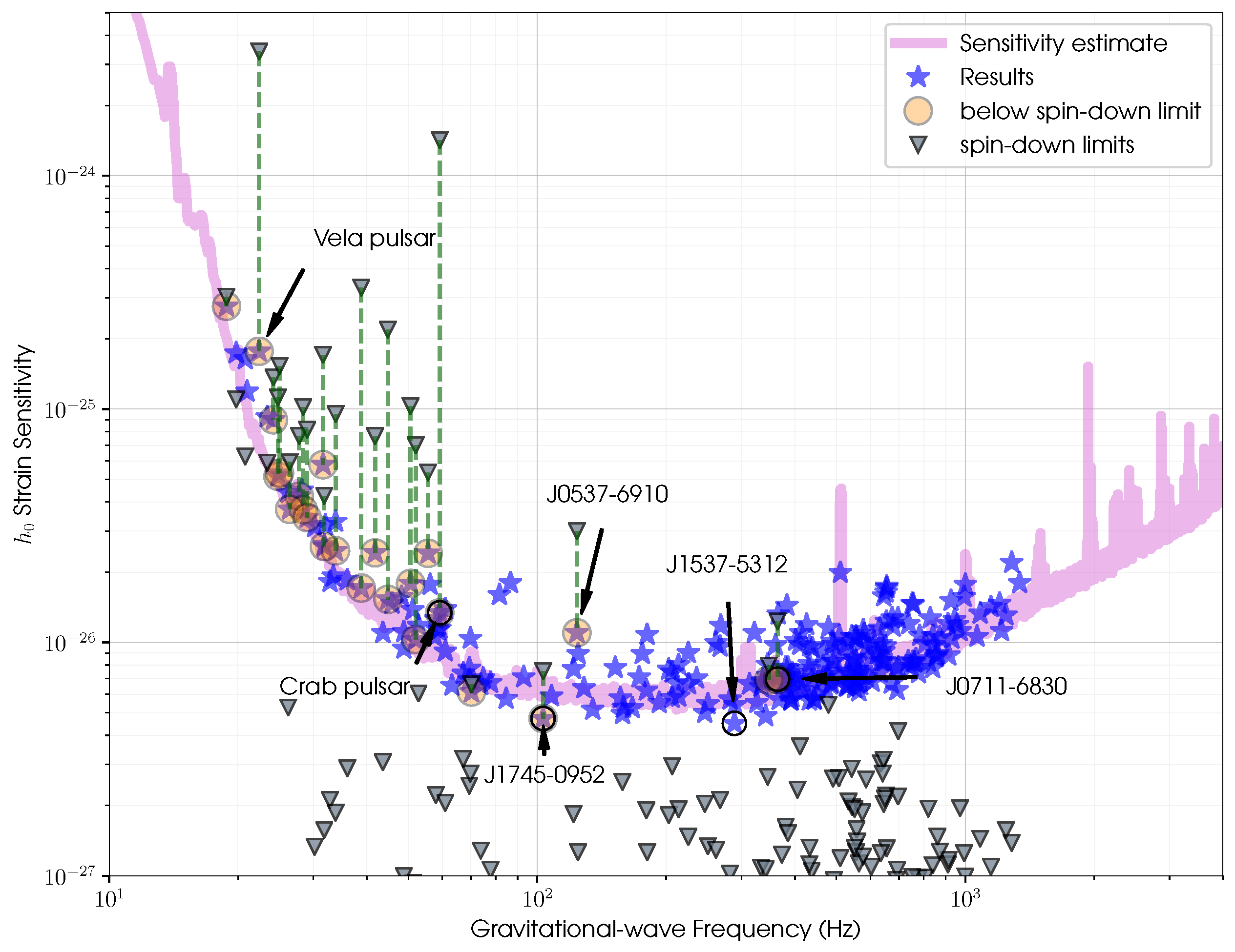
Figure 1.
This image, taken from a 2021 paper [18] by the LIGO-Virgo-KAGRA collaboration, shows the maximum amplitude of a continuous wave any of these neutron stars could emit without being found by the search analyses. Circled stars show results constraining the physical properties of specific neutron stars.
2. Dataset
2.1. Generation of Data
In this study, we employ simulations of two gravitational wave interferometers, specifically LIGO Hanford and LIGO Livingston, for the training and validation of our model. These simulations facilitate the generation of pure signal data samples and data samples that replicate real noise conditions. During the training phase, we combine the signal and noise samples using a Gaussian method, categorizing them into two distinct classes: (i) monochromatic signals embedded in pure Gaussian noise with time gaps (designated as target = 1), and (ii) signals accompanied solely by pure Gaussian noise (designated as target = 0). The data was generated utilizing the PyFstat Python package. To fulfill our experimental requirements, we produced 20,000 unique sets characterized by varying signal depths, which correspond to decreasing signal-to-noise ratios (SNR). This relationship is defined by the equation , where represents the power spectral density of the noise and denotes the signal amplitude. Additionally, we generated 20,000 spectrograms that were randomly sampled from a frequency range of 50 to 500 Hz, adhering to a uniform distribution (refer to Table 1).
Concurrently, we produced an equivalent number of simulated pure noise datasets derived from the noise data generated by the actual H1 and L1 detectors. To achieve image data of dimensions 256x360, we organized the SFT data into 256 temporal segments. For each of these 256 time segments, we generated noise that matched the amplitude observed in the source spectrogram, specifically the real noise recorded by the H1 and L1 detectors during the O3 observing run [19], which lasted several weeks to a few months. [Figure 2]
2.2. Data Processing
In numerous works, a commonly used approach to processing gravitational wave data is by converting the raw SFT data into Q-spectrograms and then doing it as a visual task.At the same time, through some previous work we note the effectiveness of the approach [23]. Therefore, in this paper, we continue to use this method to obtain spectrogram data from gravitational wave data by Q-transformation. A spectrogram is a visual representation of the spectrum of frequencies of a signal as it varies with time. A spectrogram is usually depicted as a heat map, i.e., as an image with the intensity shown by varying the colour or brightness.Between this property of the optical spectrum, our model can learn useful features better. In order to better process the data we first briefly understand the SFT, for each data sample in the dataset, where the SFT can be recovered from the existing SFT by applying the inverse SFT (i.e., restored to the time domain). A time-domain graph shows how a signal changes over time; Though most precisely referring to time in physics, the term time domain may occasionally informally refer to position in space when dealing with spatial frequencies, as a substitute for the more precise term spatial domain. The SFT is invertible, that is, the original signal can be recovered from the transform by the inverse SFT. The most widely accepted way of inverting the SFT is by using the overlap-add (OLA) method, which also allows for modifications to the SFT complex spectrum. This makes for a versatile signal processing method, referred to as the overlap and add with modifications method.
The inverse Fourier transform of for fixed:
About the Q-Transform, in mathematics and signal processing, the constant-Q transform and variable-Q transform, simply known as CQT and VQT, transforms a data series to the frequency domain. It is related to the Fourier transform and very closely related to the complex Morlet wavelet transform. Its design is suited for musical representation [16].
Next we preprocessed on the spectral data. We synchronized the spectrograms of the two detectors so that the model could capture the signal more easily without having to look around. Time-averaged bins (128-720 bins) were used as input images. At the same time, we also tried some normalization(Regularization of the spectrum ): Global regularization [15]: regularizes the whole input image by subtracting the mean and dividing by the variance. Column-wise sqrt regularization [14]: Since the background noise follows a chi square distribution, we search for the square root of the input image so that the output can follow a normal distribution, and at the same time, mitigate the effects of nonstationary noise by subtracting the mean mean, or dividing by the std (variance) in each column.
3. Comparison Test Benchmark
3.1. The Benchmark Definition
To demonstrate the efficacy of the Deep Learning Method proposed in Section 4, we utilize Table 1 as a benchmark. Concurrently, we assess the corresponding sensitivity achieved through a classical approach, specifically the match-filter search method, as detailed in Section 3.2.
We conduct a comparison of sensitivity in the Neyman-Pearson framework, commonly referred to as the receiver-operator characteristic (ROC), employing the “upper limit” conventions prevalent in continuous wave (CW) searches (see Ref [3]). This involves measuring the detection probability at a predetermined false-alarm rate for a signal sample with a fixed amplitude , while all other signal parameters (e.g., polarization, sky position, frequency, and spindown) are drawn randomly from their respective priors.
We define the sensitivity depth as a measure of the strength of signals in noise, expressed mathematically as:
where represents the power spectral density of the Gaussian noise at the signal frequency, and denotes the signal amplitude. Our focus is particularly on the sensitivity depth , which corresponds to the signal amplitude at which the search achieves a detection probability at a fixed false-alarm rate per 50 mHz frequency band.
The rationale for employing stationary white Gaussian noise is its capacity to facilitate the efficient generation of training datasets, as well as to simplify comparisons with the sensitivity of idealized matched filtering. We consider all-sky searches (as detailed in Table 1) across a range of frequencies f and spin-down rates , utilizing seconds (approximately 12 days) of data from two detectors, LIGO Hanford and LIGO Livingston. This search can be realistically executed using coherent matched filtering; however, the computational demands remain substantial. Consequently, we characterize the matched-filter search across only five narrow frequency bands, each with a width of mHz, commencing at frequencies Hz, resulting in a total of ten representative test cases [2].
3.2. Weave Matched-Filtering Sensitivity
For the Weave matched-filtering method, we use the previous Weave code [21], which implements a state-of-the-art CWs search algorithm based on a summing coherent statistics over semi-coherent segments on optimal lattice-based template banks. This code can also perform fully coherent -statistic searches. In this study, the benchmark search definition in the Table 1 are chosen in such a way that a fully coherent search is still computationally feasible. That yields a simpler comparison than using a semi-coherent search setup, as we can easily design near-optimal search setups (by using relatively fine template banks) without the extra complication of requiring costly sensitivity optimization at fixed computing cost.
The Weave template banks are characterized by a maximal-mismatch parameter m, which controls how fine the templates are spaced in parameter space. we choose the for the . The reason for choosing the large mismatch value (i.e., coarser template bank) in the case is to keep the computing cost of the corresponding test case still practically manageable.
We can measure the relative SNR loss compared to a perfectly matched template by repeated injections of signals in the data and recovery of the loudest -statistic candidate in the template bank. The resulting measured average mismatch quantifies in some sense how close to “optimal” the matched-filter sensitivity will be (compared to an infinite computing cost search with ), and is found as for the search. In order to estimate the sensitivity for the test case that was defined earlier.(i.e., five frequency slices of mHz for the search of s.) we confirmed thresholds . on the statistic corresponding to a for each case. This is done by approximate times for performing the search over Gaussian noise and thereby recording the distribution of the loudest candidate, which yields the relationship between the and . The corresponding for given any signals of fixed is obtained by injecting signals into Gaussian noise sample and measuring how many times the loudest candidate over the .As the result, we can find for the desired by varying the injected . On the other hand, we can verify that the achieved Weave detection probability for the quoted thresholds and signal’s strengths in Table 2 is .
The sky template resolution grows as as a function of frequency f, resulting in a corresponding increase in the number of templates at higher frequency. This increases the number of ’trials’ in noise in higher frequency slices, resulting in a corresponding increased false alarm threshold (chosen to keep the false alarm level at , as well as an increase in the computing cost. (See Table 2).
4. Deep Learning for Detecting CWs
In comparison to the numerous previous similar works [6,12], we settled on choosing the Efficientnet family as the backbone of our model [22], at the same time, we comparing our model to numerous types of pure CNNs models. We preenumerate multiple preprocessing layers (position-encoding-add embedding layer, position-encoding-cat embedding layer) to compare with our proposed LARGE KERNEL layer with different backbones.
At the same time, we have tried several different pooling layers (including, AdaptiveConcatPool2d, AdaptiveAvgPool2d, AdaptiveMaxPool2d, GeM) and we also have tried several attention layers (TripletAttention, ManifoldMixup).
Our model will be trained on time-frequency data from a synthetic dataset of the two gravitational wave interferometers (LIGO Hanford and LIGO Livingston) simulated by using the PyFstat [13] toolkit and tested on a synthetic dataset synthesized by the same method.
4.1. The Large Kernel Layer
In this section, we present the implementation of our proposed large kernel and the related principles. First, we will discuss the reason why we introduce the large convolutional kernel, because the convolutional kernel of the traditional convolutional neural network is generally small, which leads to the model’s view range being limited to a small field of view and makes the model not able to extract the useful features well, so we are influenced by (Scaling Up Your Kernels to 31x31: Revisiting Large Kernel Design in CNNs [5]), we decided to try to introduce a large convolutional kernel layer into CNNs to enlarge the viewing area of the model so that the model can learn to extract features better. First, our large kernel layer is realized by modifying the forward propagation process based on the original torch2d convolutional layer, as follows: First for the input, we first flatten the batch and channel dimensions to get the tensor shape as:, Then we take the absolute values of the convolution kernel weights and perform the following normalization method so that the sum of the absolute values of each convolution kernel is 1:
Then we splice the original weights and the normalized convolution kernel to form a joint convolution kernel, and we also specially create an all-1 matrix () for simulating an idealized input with all-1 centers and 0 edges that is not affected by padding, so that we can use this matrix to compute the scaling factor at a later stage, and the idea is that by constructing an all-1 matrix in order to be able to use it in the case of an all-1 input The idea is to compute the ratio of the original convolution to the normalized convolution in order to get a global scaling factor, which we can then use to scale the normalized convolution so that we can subtract this part from the output in order to reduce the impact of this part. We then perform a 2D joint convolution by applying our spliced joint convolution kernel to the convolution operation (note that, between traditional convolution operations consume a lot of computational resources, we use Fourier convolution FFtconv2d [11] for the joint convolution operation to efficiently compute the oversized convolution kernel):
Where output is the original convolution result, power is the result after normalized convolution and J stands for the joint convolution kernel hence we get:
where X were the model inputs, W were original weight matrix, were the convolutional kernel weights after normalization. We then calculate the ratio of the original convolution to the normalized convolution in the ideal state to obtain the global scaling factor :
As (beacuse of the sum of the normalized convolutions is 1) so, we get:
Next, we mitigate the disturbances caused by the bias parameters by performing a debiasing adjustment, thus enhancing the robustness:
In the above equation we achieve this operation by subtracting the effect from the bias by the original convolution. Finally, we reshape our output to get output that is the same size as the original.
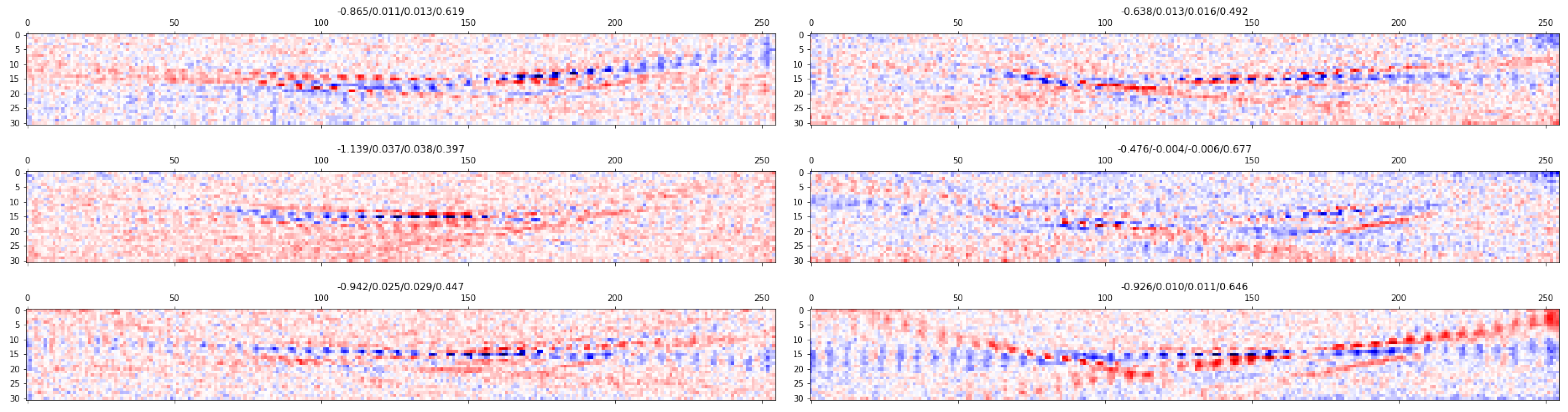
Figure 4.
Above image shows a visualization of the gravitational wave signals extracted by our LARGE KERNEL layer, thus showing that the LARGE KERNEL works well.
Figure 4.
Above image shows a visualization of the gravitational wave signals extracted by our LARGE KERNEL layer, thus showing that the LARGE KERNEL works well.
4.2. Model architecture
A huge advancement in convolutional neural networks was the ResNet (residual neural network model) proposed after AlexNet [1] and in a paper published by Kemin et al. [10] The model effectively avoids problems such as gradient vanishing by applying skips, and also extends the performance and scale of the model to a certain extent. However, with the passage of time and the demands of the real industry, we are no longer satisfied with the performance of ResNet, and so people begin to explore more efficient, more flexible, and larger model architectures, which is best represented by the work of Mingxing Tan, Quoc V. Le et al.’s work [17], which proposes a new scaling method that uses simple but efficient composite coefficients to uniformly scale all dimensions of depth/width/resolution. The model architecture EfficientNet presented in the modified work demonstrates the effectiveness of this approach in scaling MobileNets and ResNet. Another excellent strategy for reducing training time of CNNs and improving model’s accuracy is Transfer Learning [24], which capitalizes on the knowledge acquired from pre-training CNNs on a comperhensive dataset to allow us to use pre-trained models to get a good performance. Between the efficiency of this approach and Transfer Learning method, we have used it in that paper as our backbone by choosing a different EfficientNet from the pre-trained EfficientNet family.
In Figure 5 The gravitational wave spectral image data first go through a large kernel to extract the useful signal feature maps, the gravitational wave signal data undergo some denoising in this layer so that the model can better learn the useful features at a later stage, and then the feature maps are put into a pre-trained EfficientNet as a backbone for further denoising. denoising, and finally we add an attention at the end of the efficientNet in order for the model to better notice the gravitational wave signals instead of the nosie. The data stream then passes through a pooling layer (in this model we use GeMPooling as our pooling layer) to implement a dimensionality reduction operation on the data and to aggregate the features in order to prevent the risk of overfitting, and finally, the data stream is then fed into a feedforward layer with dropout to achieve binary classification. At the same time, our network architecture is highly scalable, which gives us space to optimize the network in the future.
4.3. Training and Validation
In this study, we trained our neural network using a synthesized dataset composed of input vectors that include an equal distribution of Gaussian noise (designated as target = 0) and signal data (specifically, continuous gravitational wave signals embedded within simulated real-world noise). We generated approximately 20,000 samples of pure signals, which, in conjunction with synthesized Gaussian noise, form a subset of the data samples classified as target = 1, containing continuous gravitational wave signals. The sample ratio was confirmed to be 0.66, with the injected signals characterized by random parameters and signal depths () ranging from 25 to 60.
A complete iteration through this training dataset is referred to as a training epoch. The data samples containing the signals (target = 1) utilized in the training were derived by integrating the pure continuous gravitational wave signals with the parameters specified in Table 1 and the simulated real-world noisy data. Subsequently, we partitioned the entire dataset into training and validation subsets employing K-Fold cross-validation from the sklearn toolkit. At the conclusion of each epoch, we employed the Area Under the Curve (AUC) as our evaluation metric to assess the model’s performance on the independent validation dataset. This methodological approach has proven to be significantly effective, with our architecture demonstrating superior performance relative to other models based on the AUC metric, as detailed in Table 3.
Notably, we observed that our model exhibits an "epiphany point," as illustrated in Figure 6, during the first fold across all parameters, after which the model rapidly transitions into an effective learning state. We hypothesize that this intriguing phenomenon may be attributed to the structural characteristics of the model, particularly the delayed effect of gradient propagation, which is commonly observed in deeper model architectures. Such architectures, including complex models with a substantial number of parameters, like transformers, may hinder effective gradient propagation during the initial training phases until certain layers are adequately trained (for instance, some attention mechanisms may only activate in the middle or later stages). Additionally, excessive regularization may lead to diminished gradient magnitudes, thereby inhibiting the model’s learning capacity.
In light of these conjectures, we explored various strategies, including gradient trimming to constrain the gradient within a specific range based on multiple experimental trials, substituting the attention layer, reducing model parameters, and initially employing unsupervised learning. Our findings indicate that these methods can mitigate the aforementioned phenomenon to some extent. However, due to limitations in computational resources, we have not explored other hyperparameter optimization techniques, highlighting the potential for further enhancement of our model.
5. Result
The validation of our model EPLNet on our generated dataset is shown in Figure 7.
5.1. Test on Generated Data
In our work, in order to better test the generalization ability of our model, we have validation the EPLNet with tf-EfficientNet-b5-ns as the backbone on difference signal depth Hz respectively. and finally, we choose the better performance among them for the final signal injection test. eg. i) model1: Hz, ii) model2:Hz, iii) model3: Hz. We evaluated the auc scores and RoC performance of the above three models, combining the above.(Figure 8) Finally, we chose model1 as our final model.
5.2. Test on Injected Dataset
In this study, continuous wave (CW) signals with frequencies corresponding to global and signal depths of approximately were subjected to true interferometer noise for testing purposes. A total of ten distinct signals were collected, with durations ranging from two weeks to several months. Each signal sample underwent augmentation through techniques such as time shifting, flipping, and rotation, resulting in the generation of up to 1000 unique files. Approximately half of these files contained the CW signal, while the remainder consisted solely of detector noise. As illustrated in Figure 9, the model’s performance exhibited a marked decline when tasked with predicting signal labels in the presence of real noisy data. Nevertheless, despite the challenges posed by low signal-to-noise ratio (SNR) data samples, our predictions outperformed random guessing, albeit with less consistency compared to predictions made on synthetic data. The presence of detector artifacts, including spectrograms of actual noise that resemble the signal (as depicted in Figure 2), further complicates the prediction process. This observation underscores the necessity for training the EPLNet with more realistically simulated noise for any practical application. Notably, two potential approaches can be pursued: i) initiating the training of the EPLNet with CW signals injected with real noise, or ii) employing software to generate more realistic data, such as the PyFstat package utilized in this research.
6. Discussion
In this research, we present evidence that our proposed architecture, EPLNet, is capable of effectively detecting continuous gravitational waves (CWs). This is achieved through the incorporation of a large convolutional kernel layer, referred to as LARGE KERNEL, alongside an EfficientNet backbone. We evaluate the performance of this network architecture on datasets that include CW signals superimposed on a backdrop of authentic detector noise. Furthermore, we conduct a comparative analysis of our architecture against other established models utilizing a dataset generated by PyFstat, which highlights the superior performance of our approach while also acknowledging the potential for further enhancements. We posit that with ongoing optimization and refinement, our architecture could improve its efficacy in detecting weaker gravitational wave signals. Additionally, our findings indicate that the scalability and broader field of view afforded by the large convolutional kernel, in contrast to conventional convolutional neural networks, enable the model to more effectively isolate signals obscured by noise. Consequently, the application of large convolutional kernel neural networks may represent a promising direction for future research in this domain.
References
- Krizhevsky, A.; Sutskever, I.; Hinton, G.E. Imagenet classification with deep convolutional neural networks. Commun. ACM 2017, 60, 84–90. [Google Scholar]
- Dreissigacker, C.; Sharma, R.; Messenger, C.; Zhao, R.; Prix, R. Deep-learning continuous gravitational waves. Phys. Rev. D 2019, 100, 044009. [Google Scholar]
- Dreissigacker, C.; Prix, R.; Wette, K. Fast and accurate sensitivity estimation for continuous-gravitational-wave searches. Phys. Rev. D 2018, 98, 084058. [Google Scholar]
- George, D.; Huerta, E.A. Deep learning for real-time gravitational wave detection and parameter estimation: Results with advanced ligo data. Physics Letters B 2018. [Google Scholar]
- Ding, X.; Zhang, X.; Zhou, Y.; Han, J.; Ding, G.; Sun, J. Scaling up your kernels to 31x31: Revisiting large kernel design in cnns. CVPR 2022 2022. [Google Scholar]
- Dreissigacker, C.; Prix, R. Deep-learning continuous gravitational waves: Multiple detectors and realistic noise. Phys. Rev. D 2020, 102, 022005. [Google Scholar]
- Dreißigacker, C.; Prix, R.; Wette, K. Fast and accurate sensitivity estimation for continuous-gravitational-wave searches. Physical Review D 2018, 98. [Google Scholar]
- Dreißigacker, C.; Sharma, R.; Messenger, C.; Prix, R. Deep-learning continuous gravitational waves. Physical Review D 2019, 100. [Google Scholar]
- Cuoco, E.; Powell, J.; Cavaglià, M.; Ackley, K.; Bejger, M.; Chatterjee, C.; Coughlin, M.; Coughlin, S.; Easter, P.; Essick, R. Enhancing gravitational-wave science with machine learning. Mach. Learn 2020. [Google Scholar]
- He, K.; Zhang, S.; Ren, S.; Sun, J. Deep residual learning for image recognition. CoRR 2015, abs/1512.03385. [Google Scholar]
- Huan, S. Fast fourier transform and 2d convolutions. tjhsst 2020. [Google Scholar]
- Joshi, P.M.; Prix, R. Novel neural-network architecture for continuous gravitational waves. Phys. Rev. D 2023, 108, 063021. [Google Scholar]
- Keitel, D.; Tenorio, R.; Ashton, G.; Prix, R. Pyfstat: a python package for continuous gravitational-wave data analysis. Journal of Open Source Software 2021, 6, 3000. [Google Scholar]
- Tanaka, M.; Kimura, Y.; Kudo, K. A column-wise update algorithm for nonnegative matrix factorization in bregman divergence with an orthogonal constraint. Mach. Learn 2016. [Google Scholar]
- Phan, H.; Le, T.; Phung, T.; Bui, T.A.; Ho, N.; Phung, D. Global-local regularization via distributional robustness. cs.LG 2023. [Google Scholar]
- Schrkhuber, C; Klapuri, A. Constant-q transform toolbox for music processing. Bibtex Nuhag 2010. [Google Scholar]
- Tan, M.; Le, Q.V. Efficientnet: Rethinking model scaling for convolutional neural networks. CoRR 2019, abs/1905.11946. [Google Scholar]
- the KAGRA Collaboration The LIGO Scientific Collaboration; the Virgo Collaboration. Searches for gravitational waves from known pulsars at two harmonics in the second and third ligo-virgo observing runs. LIGO-P2100049 2022. [Google Scholar]
- the KAGRA Collaboration The LIGO Scientific Collaboration; the Virgo Collaboration. Open data from the third observing run of ligo, virgo, kagra, and geo. The Astrophysical Journal Supplement Series 2023, 267, 29. [Google Scholar]
- the Virgo Collaboration The LIGO Scientific Collaboration. Gwtc-1: a gravitational-wave transient catalog of compact binary mergers observed by ligo and virgo during the first and second observing runs. Physical Review X 2019, 9. [Google Scholar]
- Wette, K.; Walsh, S.; Prix, R.; Papa, M.A. Implementing a semicoherent search for continuous gravitational waves using optimally constructed template banks. Phys. Rev. D 2018, 97, 123016. [Google Scholar]
- Zdeborová, L. Understanding deep learning is also a job for physicists. Nat. Phy. 2020, 16. [Google Scholar]
- Zhang, D. Detecting gravitational waves using constant-q transform and convolutional neural networks. In Proceedings of the 2021 4th International Conference on Computational Intelligence and Intelligent Systems, CIIS ’21, New York, NY, USA, 2022; Association for Computing Machinery. pp. 37–43. [Google Scholar]
- Zhuang, F.; Qi, Z.; Duan, K.; Xi, D.; Zhu, Y.; Zhu, H.; Xiong, H.; He, Q. A comprehensive survey on transfer learning. CoRR, 2019; abs/1911.02685. [Google Scholar]
Figure 2.
The image above shows comparison of the data we generated based on real-world noise with real noise.
Figure 2.
The image above shows comparison of the data we generated based on real-world noise with real noise.
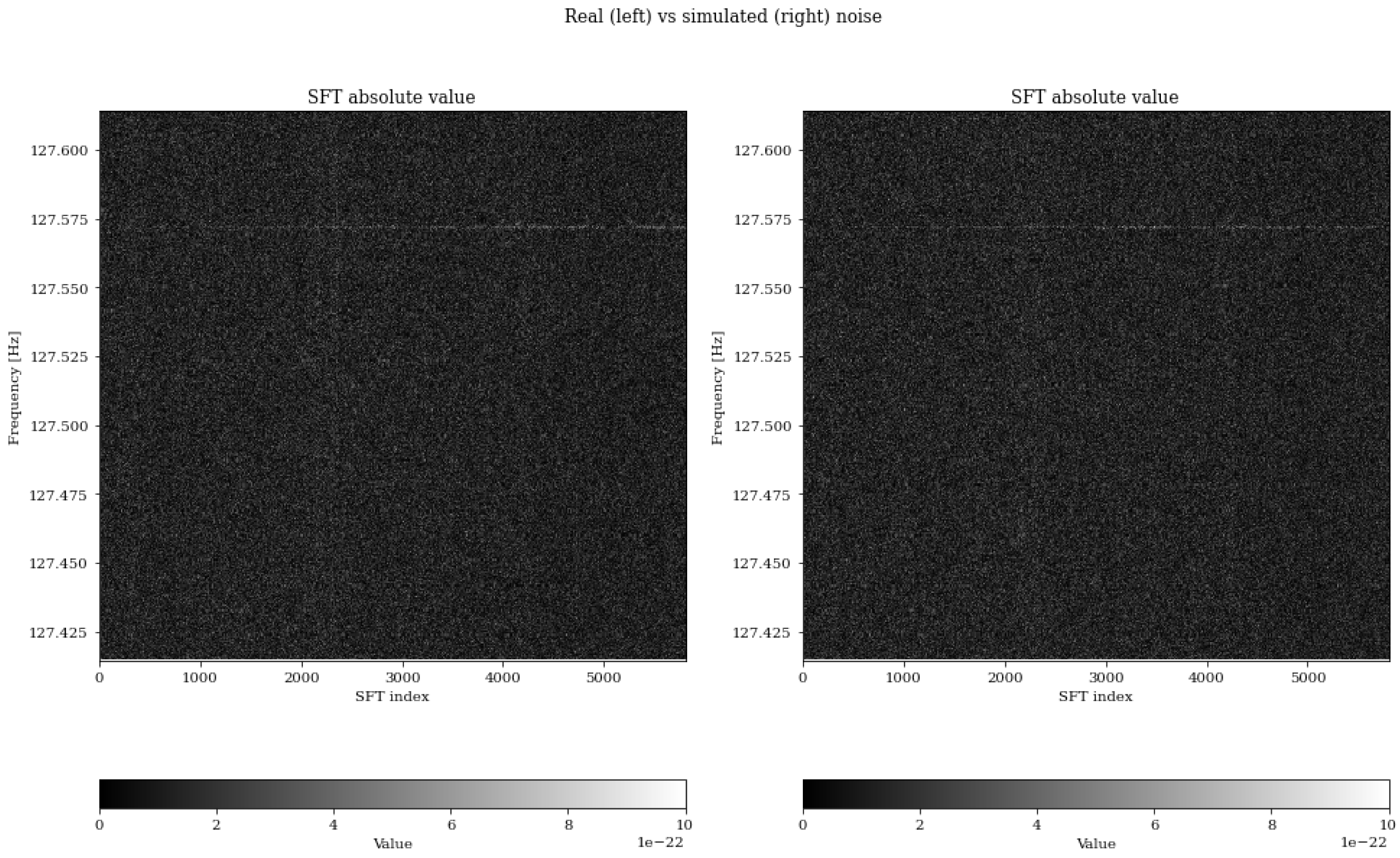
Figure 3.
The image shows some spectrograms from train dataset by constant-Q transforms.
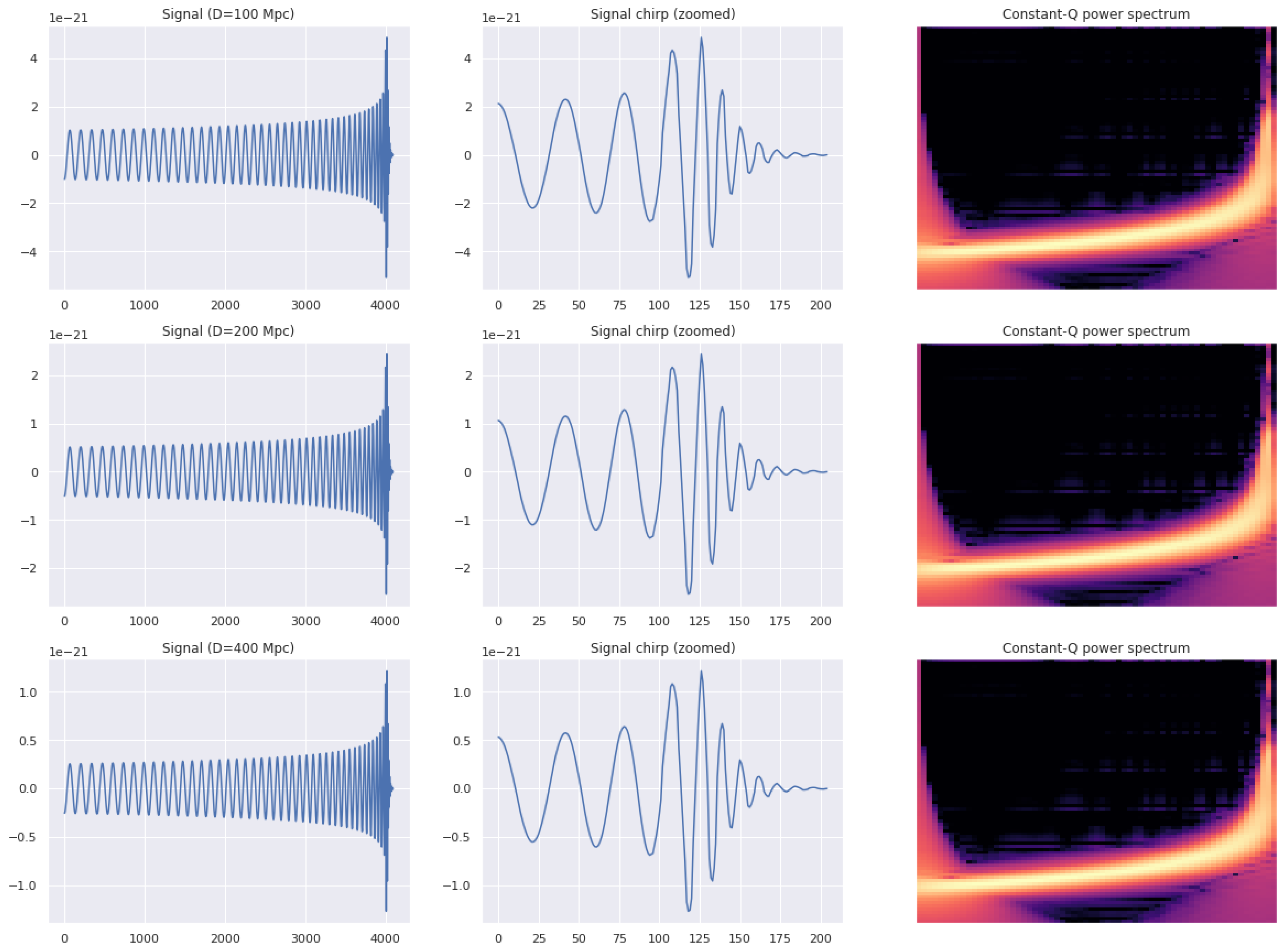
Figure 5.
The image above shows our model—EPLNet, it’s composed of processing layer(Large Kernel), backbone block (EfficientNet), Attention Layer, Global Pooling Layer.
Figure 5.
The image above shows our model—EPLNet, it’s composed of processing layer(Large Kernel), backbone block (EfficientNet), Attention Layer, Global Pooling Layer.
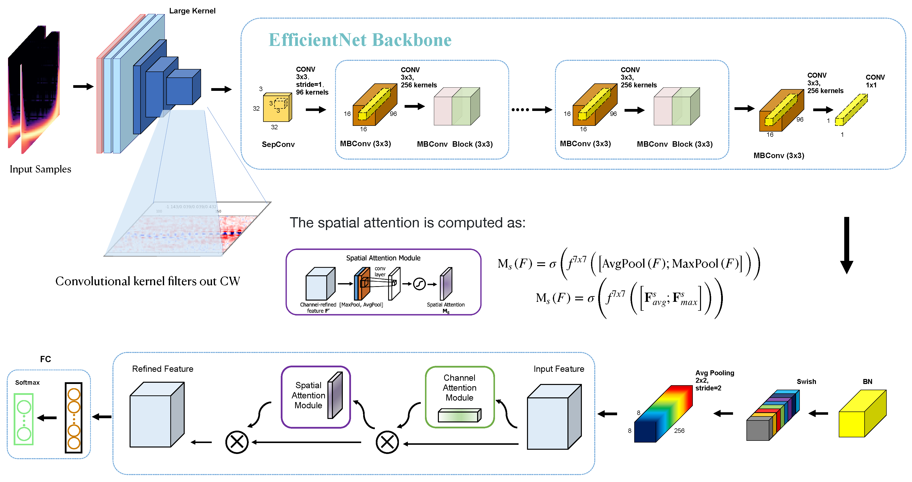
Figure 6.
The figure above shows how EPLNet’s loss decreases during training; note that the “epiphany point” at step of 2.5k.
Figure 6.
The figure above shows how EPLNet’s loss decreases during training; note that the “epiphany point” at step of 2.5k.
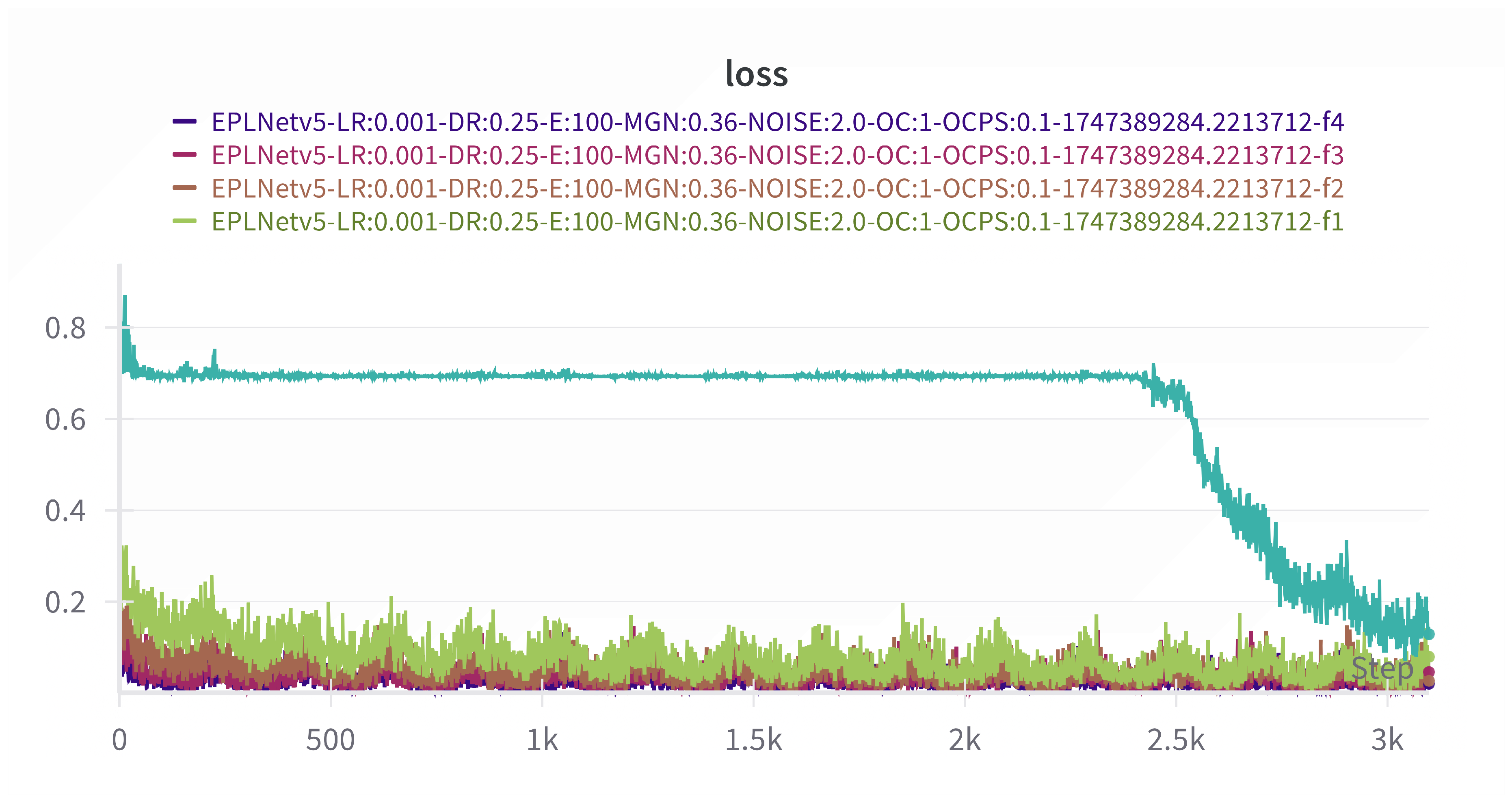
Figure 7.
The above images show the auc results of our EPLNet model (under the backbone as tf-EfficientNet-b5-ns condition) obtained after multiple rounds of cross-validation on our proposed validation set.
Figure 7.
The above images show the auc results of our EPLNet model (under the backbone as tf-EfficientNet-b5-ns condition) obtained after multiple rounds of cross-validation on our proposed validation set.
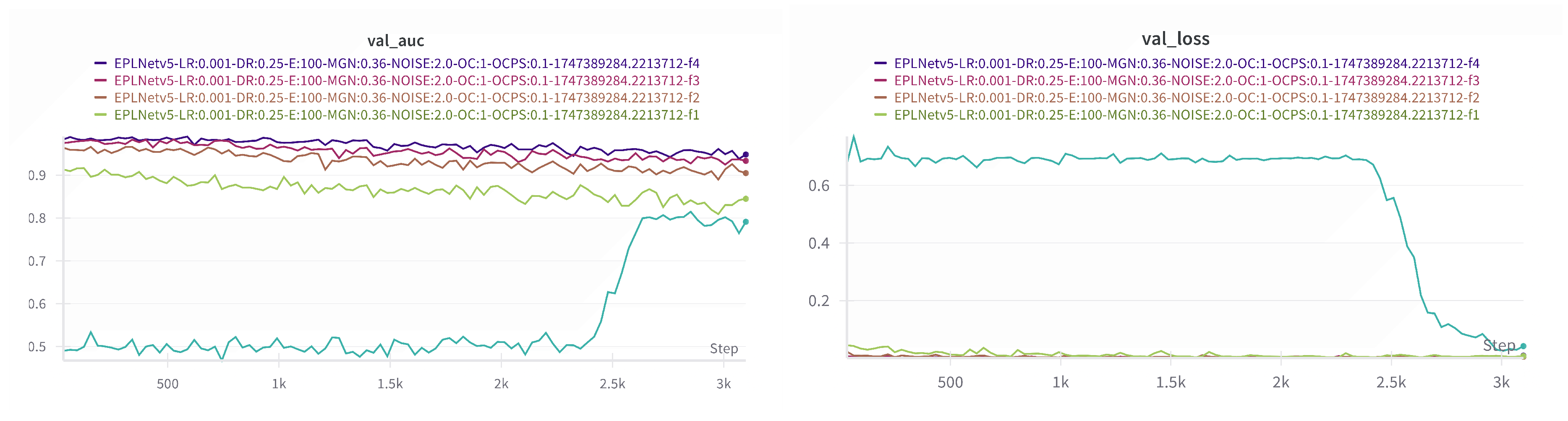
Figure 8.
The figure shows the model’s performance on different sample with different SNR.(Limited by the machine, our model is not really well trained on larger datasets, so there is still a lot of room for model enhancement.)
Figure 8.
The figure shows the model’s performance on different sample with different SNR.(Limited by the machine, our model is not really well trained on larger datasets, so there is still a lot of room for model enhancement.)
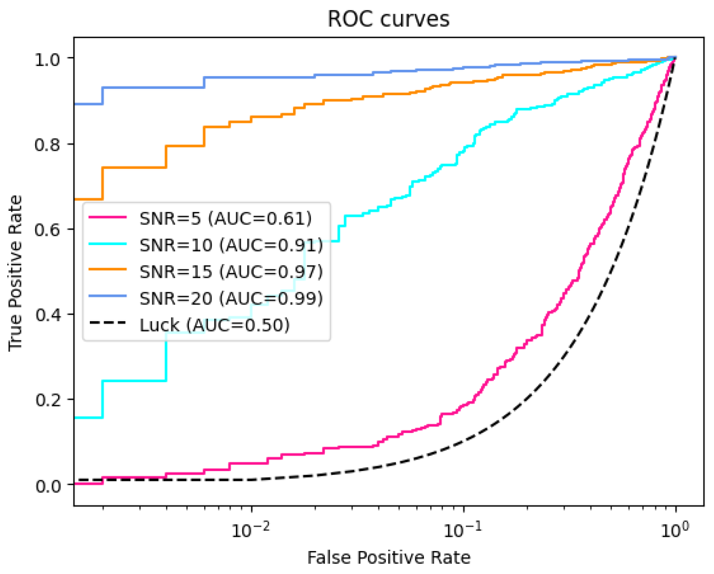
Figure 9.
The RoC curves for Model1 when evaluated on the dataset with real detector noise.
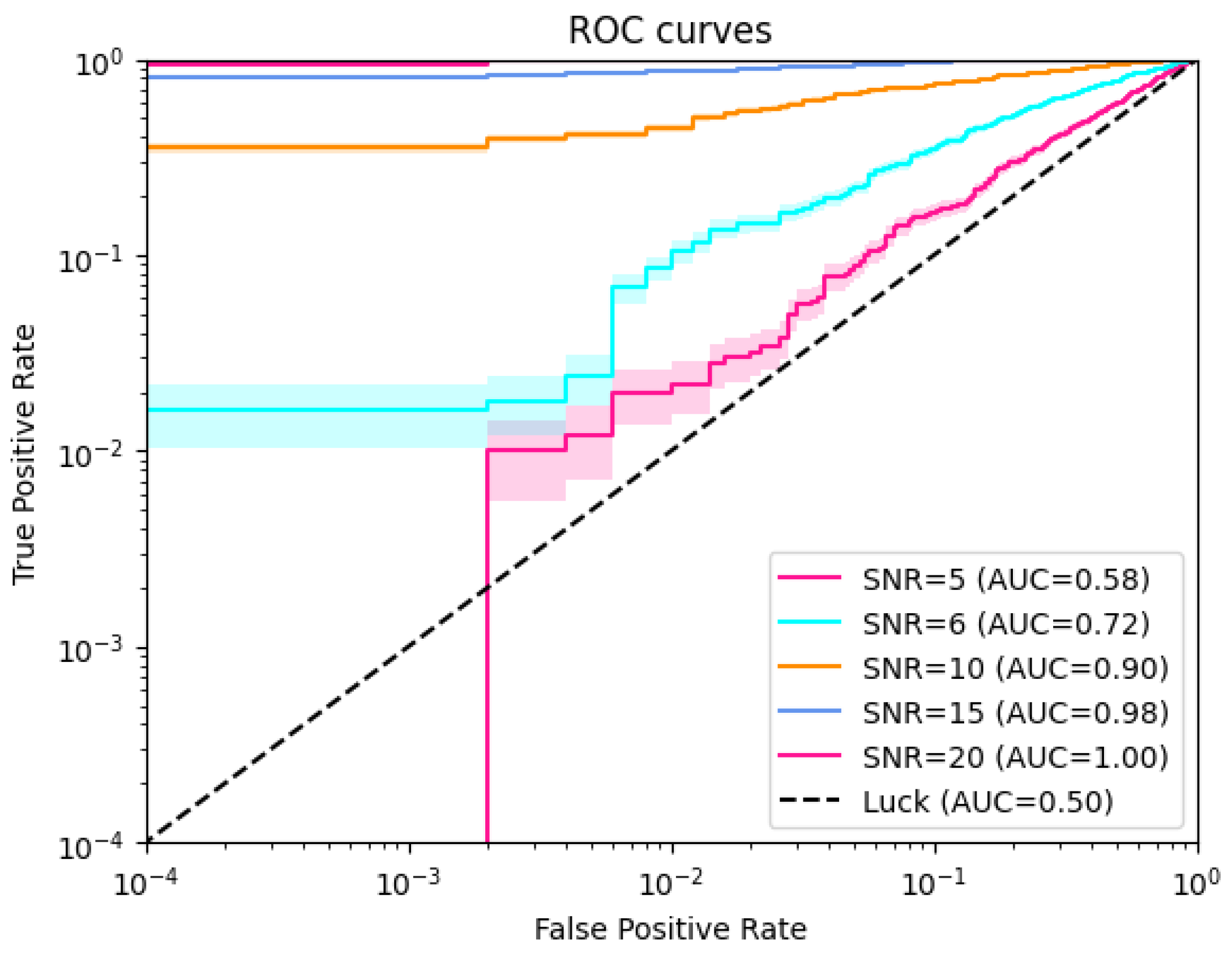

Table 1.
Definition of the parameters for synthetic Pure signals generation.
| Data span | s |
|---|---|
| Noise | Stationary, white, Gaussian |
| Sky-region | All-sky |
| Signal depth | |
| Frequency band | Hz |
| Spin-down | Hz/s, |
Table 2.
WEAVE characteristics for the ten test cases, each covering a frequency slice of mHz, starting at , of the search defined in Table 1. The detection thresholds correspond to a false-alarm level of over the band . denotes the search time in seconds for the respective band on a single CPU core.
| 50Hz | 200Hz | 300Hz | 400Hz | 500Hz | |
|---|---|---|---|---|---|
| 45 | |||||
| 27.4 | 31.1 | 32.5 | 34.2 | 36.2 |
Table 3.
Comparison of EPLNet with other related models under AUC metrics (5 Folds)
| Architecture | AUC Score | Backbone | Attention | Pooling Layer |
|---|---|---|---|---|
| EPLNet | 0.9836 | tf-EfficientNet-b5-ns | Spatial + Channel Attention | AvgPooling2D |
| EPLNet | 0.8847 | tf-EfficientNet-b5-ns | Spatial + Channel Attention | GeMPooling |
| EPLNet | 0.9043 | EfficientNet-b7 | Spatial + Channel Attention | AvgPooling2D |
| EPLNet | 0.8144 | EfficientNet-v2-b0 | Spatial + Channel Attention | GeMPooling |
| EfficientNet CWT | 0.8779 | EfficientNet-b2 | Triplet Attention | AvgPooling2D |
| EfficientNet CWT | 0.87957 | Efficientnet-b7 | Triplet Attention | AvgPooling2D |
| EfficientNet WaveNet | 0.87948 | Efficientnet-b3 | Triplet Attention | AvgPooling2D |
| Densenet WaveNet | 0.8783 | Densenet201 | Triplet Attention | AvgPooling2D |
| VIT FERQ | 0.7790 | ViT-large-patch16-224-n21k | - | - |
| tf-EfficientNet-b5-ns | 0.7846 | - | - | - |
| ResNet1d-18 | 0.7631 | - | - | - |
| Unet | 0.7898 | - | - | - |
| Xception65 | 0.7753 | - | - | - |
Disclaimer/Publisher’s Note: The statements, opinions and data contained in all publications are solely those of the individual author(s) and contributor(s) and not of MDPI and/or the editor(s). MDPI and/or the editor(s) disclaim responsibility for any injury to people or property resulting from any ideas, methods, instructions or products referred to in the content. |
© 2025 by the authors. Licensee MDPI, Basel, Switzerland. This article is an open access article distributed under the terms and conditions of the Creative Commons Attribution (CC BY) license (http://creativecommons.org/licenses/by/4.0/).
Copyright: This open access article is published under a Creative Commons CC BY 4.0 license, which permit the free download, distribution, and reuse, provided that the author and preprint are cited in any reuse.


