
Submitted:
31 May 2025
Posted:
04 June 2025
You are already at the latest version
Abstract
HIV/AIDS is a chronic disease that weakens the immune system if untreated. This study develops and analyzes an optimal control model of HIV/AIDS transmission with a saturated incidence rate to assess the effectiveness of time-dependent interventions. The model is described by seven nonlinear differential equations. We first establish that the model solutions are nonnegative and bounded. The existence and stability of equilibrium points are explored, and the effective reproduction number is derived using the next-generation matrix method. The Routh–Hurwitz criterion is applied to determine the local stability of the disease-free equilibrium, while center manifold theory is used to demonstrate the occurrence of a forward bifurcation and to analyze the local stability of the endemic equilibrium. Global stability is proven using the Castillo–Chavez method for the disease-free equilibrium and a Lyapunov function for the endemic equilibrium. Sensitivity analysis highlights the impact of parameter variations on disease dynamics, identifying the effective contact rate as the most influential parameter. The model is extended into an optimal control framework by introducing educational campaigns, screening, and antiretroviral treatment as control measures. The existence of optimal control is shown, and the Pontryagin Maximum Principle is used to derive optimal control. Numerical simulations support the theoretical findings, showing that combining multiple controls significantly reduces infection levels. A cost-effectiveness analysis identifies the combination of educational campaigns and antiretroviral treatment (Strategy C) as the most efficient intervention. Overall, the results yield important implications for formulating effective and economically sustainable HIV/AIDS intervention policies.
Keywords:
HIV/AIDS model
; saturated incidence
; forward bifurcation
; optimal control
; cost-effectiveness
MSC: 34D23; 92D23; 49J15; 37N35
1. Introduction
The Human Immunodeficiency Virus (HIV) is a virus that attacks the body’s immune system by targeting white blood cells, increasing susceptibility to infections such as tuberculosis and certain cancers, and continues to pose a serious global public health challenge, particularly when transmitted through unprotected sexual intercourse. Acquired Immunodeficiency Syndrome (AIDS) represents the most advanced stage of HIV infection, typically developing after years without treatment [1]. Prevention strategies are essential and include consistent and correct condom use, comprehensive sexual health education, and public education campaigns. Early diagnosis and the timely initiation of antiretroviral therapy (treatment) are crucial to controlling the infection and preventing progression to severe immunodeficiency, opportunistic infections, increased mortality, and reduced quality of life. Globally, an estimated 39.9 million people were living with HIV in 2023, with 1.3 million new cases. Sub-Saharan Africa remains the most affected region, accounting for over two-thirds of the global HIV burden. The global prevalence among adults aged 15-49 is about 0.6%, with women and girls representing 53% of all HIV cases [2]. Despite significant progress in expanding access to antiretroviral therapy (ART), which now reaches 30.7 million people, the HIV epidemic continues to be a major public health issue. Timely screening and widespread ART availability are crucial to reducing transmission and improving health outcomes. The global spread of the HIV/AIDS epidemic has established it as a significant worldwide issue and an increasingly urgent public health challenge. The study of HIV/AIDS transmission dynamics has great attention from both mathematicians and biologists due to the multidimensional crisis, particularly in the health sector. To effectively accelerate HIV/AIDS prevention efforts, it is essential to integrate both behavioral and biomedical control strategies [3].
Due to its ability to provide both short-term and long-term forecasts of HIV and AIDS prevalence, the mathematical modelling approach has become an essential tool in analyzing the transmission and control of HIV/AIDS. There are many models in the literature that describe the dynamics of HIV/AIDS spread using a system of nonlinear differential equations. The model in [4,5,6,7], for example, incorporates behavior control through public education campaigns. These studies concluded that such campaigns, based on the ABC (Abstinence, Be faithful, use Condoms) strategy, can effectively reduce HIV/AIDS transmission. Antiretroviral treatment plays a crucial role in mitigating the spread of diseases such as HIV/AIDS. The model in [7] integrates behavioral intervention through education campaigns with biomedical treatment during the pre-AIDS stage. It introduces compartments for individuals practicing abstinence or faithfulness, condom users, and those under treatment. Thus, a compartmental HIV/AIDS model with seven population groups was developed to assess the impact of education campaigns and pre-AIDS treatment. The study used nonlinear differential equations to analyze stability and derive the effective reproduction number. The study concludes that treatment is the most effective among the three strategies. Furthermore, studies [8,9,10] indicate that well-designed public health education campaigns significantly influence HIV/AIDS transmission dynamics by highlighting their essential role in prevention efforts.
In mathematical epidemiology, disease incidence plays an important role in the study of epidemiological mathematical models. The incidence rate of disease is the rate at which new cases of infection appear in the population due to significant contact between susceptible individuals and infected individuals. Several types of incidence rates have been introduced in classical epidemiological modeling. The incidence rate of the form is called the bilinear incidence rate. In contrast, the incidence of the form , whereis the contact rate between susceptible and infected individuals, is the number of susceptible individuals, is the number of infectious individuals, and is the total population, is known as the standard incidence rate [11]. Both types have been widely used in literature [7,8,9,10]. However, there are various reasons to modify these traditional incidence formulations. For instance, if the assumption of homogeneous mixing within the population does not hold, a nonlinear transmission function may be introduced to better reflect heterogeneous mixing and realistic population structures. A more accurate alternative is the saturated incidence rate, expressed as , which incorporates the inhibitory effect (c) associated with high levels of infective individuals. To capture the inhibitory effects arising from behavioral changes or the density of infected individuals, neither the mass action incidence nor the standard incidence function is sufficient. The saturated incidence form lies between the bilinear and standard incidence rates in terms of behavioral realism. Several mathematical models have been formulated using saturated functions to represent disease incidence or control measures such as treatment [12,13,14,15,16] and references therein.
Optimal control theory is a powerful tool for designing intervention strategies to minimize infection rates while considering implementation costs in epidemiological models [17,18]. This approach has been widely applied to HIV/AIDS dynamics. For example, Yusuf and Benyah [19] incorporated behavior change and antiretroviral therapy (ART), showing that early ART combined with behavioral interventions reduces HIV incidence and prevalence. Joshi et al. [4] emphasized the impact of information campaigns and awareness-based stratification in reducing HIV transmission. According to Safiel et al. [8], screening individuals unaware of their HIV status and treating identified cases are both effective in reducing the transmission of HIV/AIDS within a population. Building upon this framework, Okosun et al. [9] extended this by including condom use, screening, and treatment in a time-dependent control model. Through the application of optimal control theory and cost-effectiveness analysis, the research highlighted the significant impact of awareness among infectives on disease transmission and associated costs. The findings concluded that the most cost-effective intervention involves the combined implementation of all control strategies. A related study [7] also examined the impact of information campaigns and treatment using optimal control and numerical simulations, confirming treatment as the most cost-effective strategy among those evaluated. The authors suggested incorporating the progression rate from asymptomatic infection to pre-AIDS as a control variable, given its high sensitivity index. Extending this to a co-infection setting, a model in [20,21] incorporated a protected class for HIV/AIDS and pneumonia, and a model in [22] incorporated a protected class and three time-dependent control measures for HIV and Hepatitis B Virus (HBV). The results show that integrating protective classes improves intervention outcomes and resource allocation. Collectively, these studies highlight the value of optimal control and cost-effectiveness analysis in guiding public health strategies to manage the transmission of diseases other than HIV/AIDS [23,24,25,26,27,28,29].
Motivated by the above studies, this study refers to the HIV/AIDS model presented in [7] by adding a screening intervention for the unaware infected individuals and assuming a saturation incidence rate. A deterministic compartmental model is proposed to capture the dynamics of HIV/AIDS transmission, followed by a comprehensive qualitative and quantitative analysis. Specifically, the study establishes the existence and stability of the disease-free and endemic equilibria and investigates the occurrence of bifurcations and their epidemiological implications. The model is further formulated as an optimal control problem by introducing time-dependent control variables representing educational campaigns, screening of unaware infectives, and treatment of aware infectives. The pairwise effectiveness of these controls is analyzed, and the most cost-effective strategy is identified using the Incremental Cost-Effectiveness Ratio (ICER) metrics. The novelty of this study lies in the comprehensive integration of three interventions (educational campaigns, screening, and treatment) into a unified modelling framework with saturated incidence. Additionally, the study evaluates the role of preventive interventions, including antiretroviral therapy, public health campaigns, and condom use, with particular emphasis on education for susceptible individuals, screening for the unaware infected, and treatment for the aware infected. By combining rigorous mathematical analysis with optimal control and cost-effectiveness evaluation, the study provides valuable insights for designing efficient and sustainable interventions for HIV/AIDS control.
This paper is organized as follows: Section 2 describes the formulation of a deterministic model for HIV/AIDS with a saturated incidence rate. In Section 3, we conduct a detailed analysis of the model, including its basic properties, the characterization of equilibrium points, and the derivation of the effective reproduction number. The section further investigates the local and global equilibria, bifurcation phenomena, and sensitivity analysis. In Section 4, the model is extended to an optimal control framework, and Pontryagin’s Maximum Principle is employed to characterize the optimal control strategies. Section 5 presents numerical simulations based on selected parameter values to illustrate the analytical results of the model and includes a cost-effectiveness analysis of the proposed control strategies. Finally, Section 6 concludes the study with a summary of the key findings and potential directions for future research.
2. Formulation of the Model
In this section, we formulate a mathematical model for the transmission dynamics of HIV/AIDS in a population under the influence of three control strategies with a saturated incidence rate. The total human population is divided into seven compartments based on the epidemiological status of individuals, namely: is the number of susceptible individuals, is the number of educated susceptible individuals who practice abstinence or be faithful (AB behavior), is the number of educated susceptible individuals who use condoms (C behavior), is the number of unaware infective individuals, is the number of aware (screened) infective individuals, is the number of individuals receiving antiretroviral (ARV) treatment, and is the number of individuals at the critical stage of infection caused by HIV (full-blown AIDS). We consider a sexually active population, and the total population at time is given by
Educational campaigns result in the division of the susceptible individuals into three subclasses, with a proportion transitioning to and at the rate and is and where is rate of educational campaigns. Susceptible individuals are uninfected but at risk of acquiring HIV through contact with three actively infectious classes, and The treated class consists of individuals receiving antiretroviral treatment for the screened infective class. The model assumes that the transmission follows a saturated incidence rate. The number of susceptible individuals is assumed to increase at a new individuals enter the sexually active population at a constant recruitment rate Susceptible individuals are reduced by the force of infection
where is the effective contact rate, and is the modification parameter relative infectivity of individuals in and , respectively. The parameter that represents the psychological or inhibitory effect is denoted by . Moreover, susceptible individuals can become educated through education campaigns and move to the compartmentsandat a constant rate and respectively. It is further reduced by a natural death at a rate Therefore, the rate of change of the susceptible individuals with time is given by
The population of educated susceptible individuals who practice AB behavior increases as susceptible receive educational campaigns at a rate and decrease due to the force of infection at the rate where represents the effectiveness of these campaigns in promoting AB behavior. Additionally, the population is further reduced by natural death at a rate Therefore, the rate of change of susceptible individuals practicing AB behavior due to educational campaigns is given by
The population of educated susceptible individuals who practice C behavior increases as susceptible receive educational campaigns at a rate It decreases due to the force of infection at the rate where denotes the effectiveness of the campaigns in promoting C behavior. This population also declines due to natural death at a rate Therefore, the rate of change of susceptible individuals practicing C behavior because of educational campaigns is given by
The population of unaware infected individuals is generated by the force of infections and . It decreases due to screening interventions among unaware infected individuals at a rate and is further reduced by progression to full-blown AIDS at a rate as well as by natural death at a rate Thus, the rate of change of the unaware infected individuals is given by
The population of aware infected individuals increases through screening of unaware infectives at a rate This population decreases due to the intervention of antiretroviral treatment at a rate , and is further reduced by progression to full-blown AIDS at a rate and natural death at a rate Therefore, the rate of change of the aware individuals over time is given by
The population of treated infective individuals increases due to the intervention of antiretroviral treatment to aware infectives at a rate This population decreases due to progression to full-blown AIDS at a rate and natural death at a rate Therefore, the rate of change of the treated infective individuals over time is given by
The population of AIDS individuals increases due to the progression of unaware infectives, aware infectives, and treated individuals to the AIDS class, at rates and respectively. This population decreases due to natural death at a rate and further decreased by AIDS-induced death at a rate Therefore, the rate of change of the full-blown AIDS individuals over time is given by
A Compartment diagram of the HIV/AIDS model incorporating education campaigns, screening, and antiretroviral treatment interventions with saturated incidence rate is presented in Figure 1. Table 1 provides detailed descriptions of each model parameter.
Based on the compartmental diagram, the model describing the dynamics of HIV/AIDS transmission with a saturated incidence rate is represented by a seven-dimensional nonlinear system of ordinary differential equations, as shown in Equation (8).
with nonnegative initial conditions,
3. Analysis of the Model
3.1. Positivity and Boundedness of Solutions
Lemma 1.
If are nonnegative, then the solutions of the model (8) are nonnegative for all .
Proof.
To prove this, we employ a proof by contradiction to demonstrate that each state variable remains non-negative for all . Let us denote
Given that all initial conditions are nonnegative, it follows that . Without loss of generality, assume. We will use proof by contradiction to show that for all . Suppose on the contrary, that this is not the case. Then, there exists a first time such that hold
for some positive constant . From the first equation of model (8) and evaluating at , we have
Since and, this simplifies to
By the Monotonicity Theorem, it follows that for all, which contradicts the assumption in Equation (10) that. Therefore, the contradiction implies that for all Using a similar argument, it can be shown that and for all . This completes the proof. □
Lemma 2.
Solution of the model (8) with nonnegative initial values are bounded.
Proof.
Let is an arbitrary non-negative solution of the model (8) with initial conditions given in Equation (9). The total population . Now adding all the differential equations given in Equation (1) we have got the derivative of the total populationto time , we have
Next, disregarding the infections , we have determined that
Thus, for the initial condition , and by applying the Standard Comparison Theorem [30], we get
Therefore, the solutionsand of the model (8) are bounded above by . This completes the proof. □
Hence, the biologically feasible region of the HIV/AIDS model (8) is given the following positively invariant region:
3.2. Existence of Equilibrium Points
To compute the equilibrium solutions of the model (8), we set the right-hand sides of the equations for model (8) to zero.
3.2.1. Disease-Free Equilibrium (DFE) and Effective Reproduction Number
The disease-free equilibrium (DFE) of the HIV/AIDS model (8) is given by
To determine the effective reproduction number for model (8), we employ the next-generation matrix method as presented in [31]. Following the approach described in [31,32], we construct the matrix and , which represent the matrix of new infections and transition matrix between the compartments of the system, respectively. Considering the infected compartments the right-hand side of model (8) can be rewritten by
where
The matrix is the Jacobian matrix of evaluated at the disease-free equilibrium , and the matrix is the Jacobian matrix of evaluated at the disease-free equilibrium , we have
The next-generation matrix is
where
Hence, the effective reproduction number of model (8) is defined as the maximum of the absolute values of the eigenvalues of the next-generation matrix, given by
where and . Here, is the contribution to the reproduction number with intervention by unaware infective individuals , is the contribution to the reproduction number with intervention by aware (screened) infective individuals , and is the contribution to the reproduction number with treated individuals T.
When education campaigns, screening, and treatment are implemented to control and eradicate the disease, the effective reproduction number represents the average number of new infections generated by a single HIV-infected individual in a susceptible population, under the influence of these control strategies.
3.2.2. Existence of Endemic Equilibrium
In this subsection, we will find conditions for the existence of an endemic equilibrium (EE) for the model (8). Let's determine the effective reproduction number. The equilibrium of model (8) and its stability denote an arbitrary endemic equilibrium of model (8). Solving the equilibrium conditions of the model (8) at a steady state gives
where and
Substituting the value of in (17) into (18), we obtain
where
From Equation (19), one solution is corresponds to the disease-free equilibrium. Another solution is given by the roots of a cubic polynomial (20),
which is related to situations where the HIV disease persists. For the endemic equilibrium to exist, is a positive real root of the cubic polynomial (20). It is clear that (since all model parameters are nonnegative) and when . Thus, the number of possible positive real roots of the cubic polynomial (20) depends on the signs of and. By applying Descarte’s Rule of Signs to the cubic polynomial in Equation (20), the number of positive real roots can be determined. In addition, according to [7], using Cardan’s formula, the polynomial (13) has one positive real root and a pair of complex conjugate roots if the discriminant, given by
where and
Furthermore, if Equation (20) has a single positive real root, then the components of the endemic equilibrium can be obtained by substituting the value of into the expression for each state in Equation (20). This result is summarized in the following lemma.
Lemma 3.
The model (8) has a unique endemic equilibrium whenever with are the positive real roots of Equation (20).
3.3. Stability Analysis
3.3.1. Local Stability of Disease-Free Equilibrium
Theorem 1.
The disease-free equilibrium of the model (8), , is locally asymptotically stable if and unstable if .
Proof.
The Jacobian matrix of the model (8) at the disease-free equilibrium , denoted by is given as
There are seven eigenvalues of the matrix ; four of the eigenvalues are , and the remaining eigenvalues are the solutions of the following into the matrix as shown below,
The characteristic equational corresponding to is
where
As are negative, the Routh-Hurwitz Criteria depicted that, Equation (24) has three negative roots if and Thus, this is possible only . As a result, the disease-free equilibrium of the model (8), , is locally asymptotically stable in Ω if . If , the Jacobian matrix has at least one eigenvalue with a positive real part. Thus, the disease-free equilibrium is locally asymptotically unstable. This completes the proof. □
3.3.2. Global Stability of Disease-Free Equilibrium
To establish the global stability of the disease-free equilibrium , we apply the method used in [33]. To do this, let the model (8) be rewritten in the form
where is the uninfected compartments, is the infected compartments. Let , where denotes the disease-free equilibrium of model (8). To establish the global asymptotic stability of the disease-free equilibrium of model (8), the following conditions must be satisfied:
- () For is globally asymptotically stable.
- () for and is a Metzler-matrix (the off-diagonal elements ofare nonnegative).
Theorem 2.
The disease-free equilibrium points of the model is globally asymptotically stable for .
Proof.
System (8) can be written as the system (25) form, and we get , . Next, we have identified the following matrices:
From the first equation of system (25),
The Jacobian matrix of is given by
The eigen values of the matrix in system (27) are and . Since the eigenvalues of the given matrix (27) are clearly negative, then the system (26) is globally asymptotically stable. At As . Thus, condition () is satisfied and is globally asymptotically stable. Additionally, we demonstrate that satisfies the second requirements stated in (). It is clear that . We derive from the second equation in Equation (25),
B is a Metzler-matrix because all off-diagonal entries of the matrix B are not negative and
Clearly, is true, since . As a result, condition () is satisfied. Therefore, both conditions are satisfied, and the proof of Theorem 2 is completed. □
3.3.3. Global Stability of Endemic Equilibrium
To analyze the global dynamics of model (8) around the unique endemic equilibrium point , we present the following result.
Theorem 3.
If , then the endemic equilibrium of the model (8) is globally asymptotically stable in .
Proof of Theorem 3.
Let such that the endemic equilibrium exist. Furthermore, considering the following function , inspired by Muthu and Kumar [34] as follows:
By direct calculating the derivative of with respect to t along the solutions of the model (8), we have
From the right-hand sides of (5) at steady state, we have . Thus,
Clearly, because which implies . Additionally, if and only if . Hence, is a Lyapunov function on Thus, as . Therefore, the largest compact invariant set in is the singleton set . By LaSalle’s Invariance Principle [35], the unique endemic equilibrium of the model (8) is globally asymptotically stable in . The proof of Theorem 3 is completed. □
The epidemiological implication of the above result is that the HIV/AIDS epidemic will persist in the community despite education campaigns, screening, and antiretroviral treatment programs if the threshold quantity () exceeds unity.
3.4. Bifurcation Analysis
An important phenomenon in compartmental epidemiological modelling, particularly in HIV/AIDS transmission, is the occurrence of a bifurcation at the critical point where . To investigate the existence of a bifurcation for the model (8), we employ the center manifold theory as described by Castillo-Chavez and song in [33].
Theorem 4.
The HIV/AIDS model (8) exhibits a forward bifurcation at whenever holds, with
Proof of Theorem 4.
We simplify model (8) by choosing, If we set, then our model (8) can be written in the form with . Thus, we have
The characteristic equation in Equation (20) produces an eigenvalue of zero if We simplify this equation and considering stated in Equation (16), we get . By selecting as the bifurcation parameter at the point where we obtain the critical value of as follows:
The Jacobian matrix of the model (8), evaluated at the disease-free equilibrium and is given by
The characteristic equation in (32), given by , gives a simple zero eigenvalues with other six eigenvalues having negative real part. The eigenvalues of the characteristic equation are and the remaining eigenvalues are the solutions of the following characteristic equation
with as in Equation (24). The Equation (33) has negative roots () when satisfies the discriminant is positive, and .
Further, the right eigenvector associated with the zero eigenvalues is denoted by can be obtained from ,
Thus, it was chosenresults in being positive. Moreover, the left eigenvector satisfying is given by
According to Theorem 4.1 in [33], we calculate the bifurcation coefficient and , we have
and
where
It is important to highlight that the coefficient is always positive. Consequently, the local dynamics around the disease-free equilibrium point are determined by the sign of the coefficient. A backward bifurcation of system (8) occurs if is positive, whereas a forward bifurcation occurs if is negative. Alternatively, model (8) exhibits a forward bifurcation if . Thus, the proof of Theorem 4 is completed. □
To demonstrate this phenomenon in relation to the above Theorem 4, the same parameter values used in Table 1 are used and forward bifurcation diagrams are depicted in Figure 2. For this set of parameter values, the associated forward bifurcation coefficient are with and . The bifurcation parameter at the point where is.
Figure 2 illustrates the system’s behaviour as the effective reproduction number varies. When , the disease-free equilibrium (DFE) is locally asymptotically stable, as shown by the solid blue line. However, when , the DFE becomes unstable, indicated by the dashed blue line. The ascending magenta line in Figure 2 represents a stable endemic equilibrium (EE) indicating a transition from the DFE to the EE, which suggests the sustained presence of the virus in the population.
For, the applying Descartes’ Rule of Signs, along with the conditions and the cubic polynomial in Equation (24), the number of positive real roots can be determined, as summarized in Table 2. In contrast, when , no endemic equilibrium exists. Figure 2 depicts these equilibria, highlighting a forward bifurcation occurring at . In the figure, the solid blue line represents the stable disease-free equilibrium for, while the dashed blue line shows the unstable DFE for . The ascending magenta curve represents the stable branch of the endemic equilibrium . Consequently, is stable when and unstable when . Similarly, is stable for and becomes unstable for .
3.5. Sensitivity Analysis
The sensitivity analysis of model parameters is an important aspect of the present study. This analysis identifies the relevant sensitivity indices for each parameter, highlighting its role in the disease dynamics. In this section, we present a sensitivity analysis of various model parameters concerning the threshold quantity . Furthermore, this analysis helps to identify the parameters that have a significant influence on , making them potential targets for intervention. A parameter that has a significant impact on indicates its dominant role in determining the endemicity of HIV/AIDS.
Following the methods described in [36], we perform the analysis by calculating the sensitivity indices of the model parameters. To conduct the sensitivity analysis, the normalized forward sensitivity index of a variable concerning a given parameter is determined. The sensitivity index of concerning the parameter is defined by the following formula:
A parameter with a larger sensitivity index value has greater influence than a parameter with a smaller sensitivity index value. The sign of the sensitivity indices concerning a parameter indicates whether the parameter has a positive or negative effect on . Specifically, if the sign of the sensitivity indices is positive, then the value of increases as the parameter increases; conversely, if the sign of the sensitivity indices is negative, then the value of decreases as the parameter increases. The sensitivity indices of various model parameters, calculated using the expression given in (34), are presented in Table 2. The effective reproduction number of the model (8) depends on fifteen parameters, namely, and . Table 2 presents the sensitivity index values and ranks the parameters from most to least sensitive. Parameters and with positive sensitivity indices indicate that the remaining parameters have negative sensitivity indices.
Figure 3 presents the sensitivity index values of various model parameters, calculated using expression (34), and arranged in descending order from the most sensitive to the least sensitive (left to right). An absolute value of the sensitive index greater than 0.5 is considered to have a significant effect on . The most sensitive parameter is the effect-contact rate () and with a sensitivity index value given by 1. This means that if the value of is increased (decreased) by 10% while other parameter values are constant, the value of increased (decreased) by 10%. Conversely, the sensitive index value of is -0.7716, indicating that increasing (decreasing) the value of while other parameter values are constant, will be followed by a decrease (increase) in the value of by 7.716 %. The same interpretation applies to the other parameters.
We have illustrated the impact of several key parameters graphically in Figure 4. Figure 4(a) shows the effect of parameter on the transmission dynamics of HIV. According to the graph, HIV infection is eradicated when the effective contact rate is reduced to 0.0000251. This demonstrates that HIV transmission can be stopped by reducing the rate of contact between susceptible and infective individuals below this threshold.
The effects of increasing the saturation rate are evaluated through numerical simulations presented in Figure 4(b). The psychological or inhibitory effect (denoted by ) is used to assess the influence of saturation, even though it does not directly affect the effective reproduction number. The numerical results indicate that the saturation rate decreases as the inhibitory effects increase.
4. Optimal Control Model
In this section, the deterministic model (8) is developed into a control problem by considering the parameters and as continuous variables that depend on time. The optimal control parameters and conditions are considered as follows:
- The parameter represents the proportion of the susceptible subpopulation that receives the educational campaign and adopts AB (Abstinence, Be faithful) and C (use Condoms) behaviours.
- The parameter represents the proportion of the unaware infective subpopulation that receives screening per unit of time.
- The parameter represents the proportion of the aware infective subpopulation that receives antiretroviral treatment per unit time.
The control variables and are defined on the closed interval , where denotes the final time of the control implementations. By integrating the three previously described control strategies into the dynamic system (1), the corresponding system of differential equations is reformulated as follows:
with the corresponding initial conditions are given in Equation (9).
4.1. Optimal Control Problem
In this section, we analyze the behaviour of the given model by using optimal control theory. The main objective is to minimizes the number of infected individuals ( and ) and the control costs associated with the educational campaigns (), screening of the unaware infective subpopulation (), and antiretroviral therapy for the aware infective subpopulation (). The objective functional for a fixed time , given by
where are nonnegative weight constant on the unaware and aware infected individuals, whereas are the relative costs of the controls associated control .
The main goal of this part is to find the optimal control strategies , subject to (35) and minimizing the objective functional Eq (36) such that
where is the control set.
4.2. Existence of an Optimal Controls
This section investigates the existence of an optimal control triple that minimize the objective functional J defined in Equation (36). To establish this, we employ the existence theorem by Fleming and Rishel [37].
Theorem 5.
Given the objective functional J defined on the control set U, there exists an optimal control triple such that Equation (37) is satisfied, provided the five following conditions hold [37]:
- (i)
- The optimal control set, and state variables set are nonempty.
- (ii)
- The control set U is closed and convex.
- (iii)
- The right-hand side of the state system (35) is continuous and bounded by a linear function in both the state and control variables.
- (iv)
- The integrand of the objective functional J in Equation (36) is convex concerning the control set U.
- (v)
- There exist constants and such that the integrand of the objective functional J in (36) is bound below by
Proof.
We must confirm the validity of the fife conditions specified in Theorem 5.
(i) Clearly, U is a nonempty set of measurable functions in, and the corresponding solutions exist and remain bounded.
(ii) Given the control set . This set can be expressed as , where each , indicating U is bounded for all . Consequently, U is closed. Now, let and any two arbitrary elements in U. By the definition of a convex set [38], it follows that for all Hence, which implies that U is a convex set.
(iii) Let be the state variables of the model (8) and Then the right-hand side of the system (35) can be written as where
Derived from the Euclidean norm of a matrix as indicated in [26,28], we obtain . This means that the right-hand side of the model (8) can be expressed as a linear function of the controls and with coefficients depending on state variables.
(iv) The integrand of the objective functional (36) can be expressed in the form of a Lagrangian as . To establish convexity, it is sufficient to show that the term is convex on the control set U. Notice that is formed as a finite linear sum of the functions . Therefore, it is easier to show that the function given by is convex. Let and . Then,
Hence, Thus, the condition satisfies the definition of a convex function as stated in [45]. As a result, the functionis convex function on U.
(v) By applying the Lagrangian equation , we demonstrate the final condition as follows:
where and .
The proof of Theorem 5 is completed. □
4.3. Characterization of the Optimal Control
We characterize the optimal control triple of the system and the corresponding states with its control function and , with the objective functional Equation (36). Using Pontryagin’s Maximal Principle [8,9], we obtain the necessary conditions for the optimal controls. Pontryagin’s Maximal Principle convert Equation (35) and Equation (37) into a problem of minimizing pointwise a Hamiltonian, concerning and . The Hamiltonian is defined as follows:
where and are the adjoint variables.
The following result gives the necessary conditions for the optimal control.
Theorem 6.
Given an optimal controls that minimizes the objective functional J over the control set U subject to system (1), then there exist the adjoint variables and satisfying the following equations:
Furthermore, the optimal, denoted as
is expressed as follows:
Proof.
We apply Pontryagin’s Maximum Principle to derive the adjoint variables, the transversality conditions, and the optimal control triplet. The system of adjoint equations (39) is obtained by taking the partial derivatives of the Hamiltonian in Equation (38) with respect to the corresponding state variables, as follows:
Finally, the optimal controls can be characterized fromin Equation (38) by applying the optimality conditions for each control measure where , for Thus,
By solving Equation (41) with the optimal controls and , we derive the following characterization:
Since all three control measures are bounded between 0 and 1, we have
where
Hence, for these controls and given in the Equation (40) are characterized by
The proof of Theorem 6 is complete. □
5. Numerical Simulations and Cost-Effectiveness Analysis
5.1. Numerical Simulation of Model
In this section, we present several numerical simulations of the model (8) to illustrate the dynamics of HIV transmission, using the parameter values estimated and shown in Table 2. These results aim to explore the dynamic effects of education, screening, and therapy interventions on HIV incidence. To perform the simulations, both models are solved numerically using the fourth-order Runge-Kutta method and implemented in MATLAB. We set the initial population as follows:
First, we set parameter value and the other parameters as given in Table 1. We obtain . Theorem 1 is numerically illustrated in Figure 5, demonstrating the global stability of the DFE within its region of attraction in both the and spaces. Figure 5(a) shows that all solution trajectories starting within the area of attraction converge to the point . Similarly, Figure 5(b) indicates that all trajectories originating within the region of attraction tend toward the point Three different initial values are used in constructing the stability diagram of in three different state spaces, as follows: (20000, 40000, 30000, 2000, 1500, 1000, 1000), (22000, 42000, 32000, 2500, 2000, 2000, 1000), (24000, 44000, 34000, 3000, 2500, 2500, 2000), and (25000, 45000, 35000, 3500, 3000, 3000, 2500). This approach can also be extended to demonstrate the global asymptotic stability of the disease-free equilibrium in other subspaces of the model.
Second, we set parameter value while the remaining parameters are taken from Table 1. This results in the effective reproduction number of Theorem 2 is numerically illustrated in Figure 6, demonstrating the global stability of the endemic equilibrium within its region of attraction in both the and spaces. In Figure 6(a), all solution trajectories that begin within the region of attraction andconverge to the point. Figure 6(b) indicates that all trajectories that begin within the region of attraction tend toward the point This methodology can further be applied to verify the global asymptotic stability of the endemic equilibrium in other subspaces of the model.
5.2. Optimal Control Simulation
We compute the numerical solution to the optimal control problem by solving the optimality system, which consists of the state and adjoint equations, using the forward-backward sweep method. This involves numerical integration using the fourth-order Runge-Kutta method implemented in MATLAB. Initially, the state system (35) is solved forward in time, with initial values determined by the transversality condition. Subsequently, the adjoint system (39) is solved backwards in time, utilizing the current iteration of state variables. The control variables are updated through a convex combination of their previous values and the new estimate derived from Equation (40). This iterative process is repeated until convergence of the state equations is achieved [18].
For numerical simulation purposes, the weight factors and are utilized, alongside cost coefficients and . Simulations were conducted over a period of 5 years. These cost values are determined based on the efforts to implement the strategies under consideration. The parameter values presented in Table 1 and are employed in the simulations for cases where . To assess the impact of various optimal control strategies on the spread of HIV infection within the community, we will examine and compare the numerical results of interventions that implement multiple strategies. Strategies involving a single intervention are excluded, as they do not ensure the complete eradication of the disease from the community. This study considers the following four combined intervention strategies:
- Strategy A: Educational campaign combined with screening
- Strategy B: Educational campaign combined with treatment
- Strategy C: Screening combined with treatment
- Strategy D: Implementation of all control
5.2.1. Simulation for Strategi A
By implementing the triple control strategies simultaneously, we observed that Strategy A, which involves the simultaneous implementation of educational campaign control (), screening control (), and antiretroviral treatment control (), significantly reduces the number of infected individuals (Figure 7). Specifically, at the final time (), the total number of unaware infectives under control is 36.7, compared to 1351.2 without control (Figure 7(a)). Similarly, the total number of aware infectives at time is reduced to 105.36 with control, whereas it reaches 4648.5 in the absence control, which is significantly different (Figure 7(b)). Additionally, the total number of individuals with AIDS at time is reduced to 269.8 with control, whereas it reaches 693.5 in the absence of control. These results demonstrate that the optimal control strategy is highly effective for both groups of HIV-infected individuals and AIDS cases. Furthermore, Figure 7(d) illustrates the control profiles for Strategy A over time. To minimize the number of HIV infections and associated costs, the control is maintained at its upper limit for approximately 2.98 years before gradually decreasing to zero at the end of the control period. Similarly, the controls and are kept at their upper limit for 2.98 years and 4.35 years, respectively, before dropping to their lower bounds at the end of the control period.
5.2.2. Simulation for Strategi B
This strategy implements both intervention measures (educational campaign control) and (screening controls). It is observed from Figure 8(a) to 8(c) that due to this control strategy, the number of unaware infectives, aware infectives, and AIDS individuals decreased only slightly during the control period. This result shows that the Strategy B has no significant effect on the subpopulation of the unaware infected individuals, aware infected individuals, and AIDS individuals. The control profile for the educational campaigns control at the beginning of the control period is at 0.53, then gradually decreases to zero at the end of the control period, while the control profile for screening control is maintained at its lower bound for the whole period (Figure 8(d)) .
5.2.3. Simulation for Strategi C
The simultaneous implementation of double control strategies demonstrates that Strategy C (i.e., applying educational campaign control and antiretroviral treatment) significantly reduces the number of infected individuals (Figure 9). Specifically, at the final time, the total number of unaware infectives under control is 9.7, compared to 1351.2 without control (Figure 9(a)). Similarly, the total number of aware infectives at time 5 years is reduced to 118.2 with control, whereas it reaches 4648.5 in the absence control, which is significantly different (Figure 9(b)). Additionally, at the final time, applying Strategy C leads to a significant decrease in the number of AIDS individuals (267.6) compared to the uncontrolled case (Figure 9(c)). Furthermore, Figure 9(d) illustrates the control profiles for Strategy C over time. The control profiles for the educational campaigns control at the beginning of the control period; it is at 0.09 then gradually decreases to zero at the end of the control period. The control profiles for the antiretroviral treatment control should be maintained at it upper bound for the first 4.4 years. After which both controls gradually decrease to it lower bound at the end of the period (Figure 9(d)). The optimal control profiles for and in Strategy C are identical to those in Strategy A.
5.2.3. Simulation for Strategi C
The simultaneous implementation of double control strategies demonstrates that Strategy C (i.e., applying educational campaign control and antiretroviral treatment) significantly reduces the number of infected individuals (Figure 8). Specifically, at the final time, the total number of unaware infectives under control is 9.7, compared to 1351.2 without control (Figure 8(a)). Similarly, the total number of aware infectives at time 5 years is reduced to 118.2 with control, whereas it reaches 4648.5 in the absence control which is significantly different (Figure 9(b). Additionally, at the final time, applying Strategy C leads to a significant in the number of AIDS individuals (267.6) compared to the uncontrolled case (Figure 9(c)). The control profiles for the educational campaigns control at the beginning of the control period it is at 0.09 then gradually decreases to zero at the end of the control period. The control profiles for the antiretroviral treatment control should be maintained at its upper bound for the first 4.4 years. After which both controls gradually decrease to its lower bound at the end of the period (Figure 9(d)). The optimal control profiles for and in Strategy C are identical to those in Strategy A.
5.2.4. Simulation for Strategi D
This strategy implements both intervention measures (screening control) and (antiretroviral treatment). Specifically, at the final time (5 years), the total number of unaware infectives under control is 36.7, compared to 1351.2 without control (Figure 10(a)). Similarly, the total number of aware infectives at time is reduced to 105.3 with control, whereas it reaches 4648.5 in the absence control, which is significantly different (Figure 10(b)). Additionally, at the final time, applying Strategy A leads to a significant decrease in the number of AIDS individuals (269.8) compared to the uncontrolled case (Figure 10(c)). The control profiles for the screening control should be maintained at it upper bound for the first 2.98 years, while the control profile for the antiretroviral treatment control () should be maintained at it upper bound for the first 4.36 years. After which both controls gradually decrease to it lower bound at the end of the period. The optimal control profiles for and in Strategy D are identical to those in Strategy A.
5.3. Cost-Effectiveness Analysis
To determine which control strategy is most effective, this subsection evaluates the economic implications of educational campaign strategies for susceptible individuals, screening for unaware infectives, and antiretroviral therapy for aware infectives in the dynamics of HIV/AIDS, using cost-effectiveness analysis (CEA). CEA helps identify and propose the most efficient or cost-effective strategy for implementation under limited sources. In this study, the evaluation will be conducted using the incremental cost-effectiveness ratio (ICER), which compares the difference in costs and health outcomes between two competing intervention strategies. Each intervention is compared to the next less effective alternative in terms of the number of infections averted [9]. When comparing two competing intervention strategies, p and q, The ICER is defined as follows [21,25].
The total averted infections, used in the cost-effectiveness analysis table, is determined by the difference between the total number of infected individuals without any control and the total number with the implementation of a control strategy. The total cost associated with a control strategy is directly proportional to the number of controls applied. In this study, the ICER values were computed using formula (31). Specifically, the total cost (TC) and total averted infections (TA) for each strategy were calculated using the following formulas:
Table 3 presents the control strategies ranked in ascending order of total averted infections. Here, the ICER is calculated for Strategies B and D to enable a comparative evaluation of their relative effectiveness, defined as:
Table 3 presents a summary of the ICER calculations of Strategies B, D, A, and C. From the table, the comparison between Strategy B and Strategy D shows that the ICER of Strategy B is higher than that of Strategy D, indicating that Strategy B is both more costly and less effective. Consequently, Strategy B should be excluded from the set of alternative control intervention strategies competing for the same limited resources. Furthermore, the ICER for Strategies D and A are recalculated using the same procedure, as presented in the fourth column of Table 4.
From Table 4, the comparison between Strategy D and Strategy A shows that the ICER of Strategy A is higher than that of Strategy D, which indicates that Strategy A is both more costly and less effective. Consequently, Strategy A should be excluded from the set of alternative control intervention strategies competing for the same limited resources. Furthermore, the ICER for Strategies D and C are recalculated, with the results presented in the fourth column of Table 5.
The comparison of ICER values for intervention Strategies D and C, as shown in Table 5, indicates that the ICER for Strategy D is higher than that of Strategy C. Consequently, Strategy D is excluded from the set of remaining alternative strategies to prevent the inefficient allocation of limited resources. We observed that Strategy C, which involves the simultaneous implementation of educational campaigns and antiretroviral treatment measures (i.e., and ), is identified as the most cost-effective among the four proposed control strategies aimed at reducing and controlling the spread of HIV/AIDS in the community considered in this study.
5. Conclusions
In this study, we developed a mathematical model for HIV/AIDS dynamics using a system of seven nonlinear differential equations. The study incorporated educational campaigns for susceptible, screening of unaware infectives, and antiretroviral treatment formulated to describe the dynamics of HIV transmission with a saturated incidence. We performed a detailed mathematical analysis of our model, including the proof of positivity and boundedness of the model solutions, established using differential equation theory. By analyzing the system, we derive the effective reproduction number using the next-generation matrix method. The existence of the disease-free equilibrium point (DFE) and the endemic equilibrium point (EE) are shown. The EE components can be determined by substituting the positive real root of the cubic equations. When applied to cubic polynomials, Descartes’ Rule of Signs allows one to determine the number of positive real roots. Based on the analysis, the Routh-Hurwitz criterion confirms the local stability of the DFE, while the application of center manifold theory reveals the presence of a forward bifurcation. Our bifurcation analysis demonstrates that the model consistently exhibits a forward bifurcation when the effective reproduction number is equal to one. The presence of a forward bifurcation also provides some information on the local stability of the endemic equilibrium. The global asymptotic stability of the DFE is established when the effective reproduction number is less than one, using the Castillo-Chavez method. Meanwhile, the global stability of the EE is analyzed through the Lyapunov function and LaSalle’s Invariant Principle.
Based on the sensitivity analysis and numerical results, this study suggests that HIV infections can be reduced by lowering the contact rate and increasing the rates of screening, educational campaigns, and antiretroviral treatment. To mitigate HIV transmission, multiple time-dependent optimal control strategies are considered, including educational campaigns (ABC strategy), screening of unaware infected individuals, and antiretroviral treatment of aware infected individuals. A thorough analysis of the model is performed to explicitly establish the existence and characterize the optimal control triple using optimal control theory, guided by the Pontryagin Maximum Principle (PMP). To achieve a comprehensive understanding of the impact of three time-dependent functions on HIV/AIDS transmission dynamics, all possible control combinations are systematically categorized into four strategies. The results indicate that various combinations of control measures can significantly reduce the number of infective individuals in the population. Furthermore, the cost-effectiveness analysis using ICER identifies the combination of educational campaigns and antiretroviral treatment of aware infective individuals (Strategy C) as the most cost-effective intervention among the four strategies examined.
This study employs a classical-order optimal control model, but research shows that fractional-order models more effectively capture real-life phenomena. Future work will extend the model to a fractional-order framework to account for memory effects in HIV/AIDS transmission dynamics.
Author Contributions
Conceptualization, M.M. and T.T.; methodology, M.M. and T.T.; software, M.M.; validation, M.M. and R.R.M.; formal analysis, M.M., T.T. and R.R.M; investigation, M.M., T.T. and R.R.M.; resources, M.M. and T.T.; writing— original draft preparation, M.M. and R.R.M.; writing—review and editing, M.M., T.T. and R.R.M.; visualization, M.M. All authors have read and agreed to the published version of the manuscript. All authors have read and agreed to the published version of the manuscript.
Funding
This research received no external funding.
Data Availability Statement
No external data were used in this study.
Acknowledgments
The author wishes to thank the handling editor and the anonymous referee for their valuable comments and constructive suggestions.
Conflicts of Interest
The authors declare no conflicts of interest.
References
- World Health Organization (WHO): Global strategic direction on HIV/AIDS 2024. Available online: https://www.who.int/observatories/global-observatory-on-health-research-and-development/analyses-and-syntheses/hiv-aids/global-strategic-direction (accessed on 17th February 2025).
- UNAIDS. (2024). Global HIV & AIDS statistics-Fact sheet. Joint United Nations Programme on HIV/AIDS. https://www.unaids.org/en/resources/fact-sheet (accessed on 17th February 2025).
- Bekker, L.G.; Beyrer, C.; Quinn, T. C. Behavioural and biomedical combination strategies for HIV prevention. Cold Spring Harb. Perspect. Med. 2012, 2, a007435. [CrossRef]
- Joshi, H.R.; Lenhart, S.; Hota, S.; Agusto, F. Optimal Control of an SIR Model with Changing Behavior through an Education Campaign. Electron. J. Differ. Equ. 2015, 50,1-14. http://ejde.math.txstate.edu.
- Hota, S.; Agusto, F.; Joshi, H.R.; Lenhart, S. Optimal control and stability analysis of an epidemic model with education and treatment. Conferensi Publication, 2015, 2015(special), 621-634. https://www.aimsciences.org/article/doi/10.3934/proc.2015.0621.
- Mukandavire, Z.; Garira, W. Effects of Public Health Educational Campaigns and the Role of Sex Workers on the Spread of HIV/AIDS among Heterosexuals. Theor. Popul. Biol. 2007, 72, 346-365. [CrossRef]
- Marsudi; Trisilowati; Suryanto, A.; Darti, I. Global stability and optimal control of an HIV/AIDS epidemic model with behavioral change and treatment. Eng. Lett. 2021, 29, 575-591. https://www.engineeringletters.com/issue_v29/issue_2/EL_29_2_26.pdf.
- Safiel, R.; Massawe, E.S.; Makinde, O.D. Modelling the effect screening and treatment on transmission of HIV/AIDS infection in a population. Am. J. Math. Stat. 2012, 2, 75-88. [CrossRef]
- Okosun, K.O.; Makinde, O.D.; Takaidza, I. Impact of optimal control on the treatment of HIV/AIDS and screening of unaware infectives. Appl. Math, Modelling, 2013, 37, 3802-3820. [CrossRef]
- Kateme, E.L.; Tchuenche, J.M.; Hove-Musekwa, S.D. HIV/AIDS Dynamics with Three Control Strategies: The Role of Incidence Function. ISRN Appl. Math. 2012, 864795. [CrossRef]
- Khan, M.A.; Ismail,M.; Ullah, S.; Farhan, M. Fractional order SIR model with generalized incidence rate. AIMS Math. 2020, 5, 1856-1880. [CrossRef]
- Khan, M.A.; Khan, Y.; Islam, S. Complex dynamics of an SEIR epidemic model with saturated incidence rate and treatment. Physica A. 2018, 493, 210-227. https://www.sciencedirect.com/science/article/abs/pii/S0378437117310488.
- M. M. Ojo. Mathematical modelling of disease dynamics with saturated incidence and treatment response. Math. Biosci. 2021, 340, 108686. http://doi.org/10.1016/j.mbs.2021.108686.
- Hu, Y.; Wang, H.; Jiang, S. Analysis and optimal control of a two-strain SEIR epidemic model with saturated treatment rate. Mathematics 2024, 12, 3026. [CrossRef]
- Olaniyi, S.; Kareem, G.G.; Abimbade, S.F.; Chuma, F.M.; Sangoniyi, S.O. Mathematical modelling and analysis of autonomous HIV/AIDS dynamics with vertical transmission and nonlinear treatment. Iran. J. Sci. 2024, 48, 181-192. [CrossRef]
- Allali, K.; Balde, M.A.M.T.; Ndiaye, B.M. An optimal control study for a two-strain SEIR epidemic model with saturated incidence rates and treatment. Discrete Dyn. Nat. Soc. 2025, 2025, 8553106, 16 pages. [CrossRef]
- Pontryagin, L.S.; Boltyanskii, V.G.; Gamkrelidge, R.V.; Mishchenko, E.F. Mathematical Theory of Optimal Processes, 1st edition, Routledge: London, 1987.
- Lenhart, S.; Workman, J.T. Optimal Control Applied to Biological Models, 1st edition, Chapman and Hall/CRC: New York, 2007.
- Yusuf, T.T.; Benyah, F. Optimal strategy for controlling the spread of HIV/AIDS disease: A case study of South Africa. J. Biol. Dyn. 2012, 6, 475-494.
- Teklu, S.W. Investigating the effects of intervention strategies on pneumonia and HIV/AIDS co-infection model. Biomed Res. Int. 2023, 5778209. [CrossRef]
- Teklu, S.W.; Terefe, B.B.; Mamo, D.K.; Abebaw, Y.F. Optimal control strategies on HIV/AIDS and pneumonia co-infection with mathematical modelling approach. J. Biol. Dyn. 2024, 18, 2288873. [CrossRef]
- Teklu, S.W.; Workie, A.H. A dynamical optimal control theory and cost-effectiveness analysis of the HBV and HIV/AIDS co-infection model. Front. Public Health 2024, 12, 1444911. [CrossRef]
- Berhe, H.W.; Makinde, O.D.; Theuri, D.M. Co-dynamics of measles and dysentery diarrhea diseases with optimal control and cost-effectiveness analysis. Appl. Math. Comput. 2019, 347. [CrossRef]
- Olaniyi, S.; Okosun, K.O.; Adesanya, S.O.; Lebelo, R.S. Modelling malaria dynamics with partial immunity and protected travellers: optimal control and cost-effectiveness analysis. J. Biol. Dyn. 2020, 14, 90-115. [CrossRef]
- Asamoah, J.K.K.; Yankson, E.; Okyere, E.; Sun, G.Q.; Jin, Z.; Jan, R. et al. Optimal control and cost-effectiveness analysis for dengue fever model with asymptomatic and partial immune individuals. Results Phys. 2021, 31, 104919. [CrossRef]
- Asamoah, J.K.K.; Okyere, E.; Abidemi, A.; Moore, S.E.; Sun, G.Q.; Jin, Z. et al. Optimal control and comprehensive cost-effectiveness analysis for COVID-19. Results Phys. 2022, 33, 105177. [CrossRef]
- Appiah, R.F.; Jin, Z.; Yang, J.; Asamoah, J.K.K. Optimal control and cost-effectiveness analysis for a tuberculosis vaccination model with two latent classes. Model. Earth Syst. Environ. 2024, 10, 6761-6785.
- Engida, A; Gathungu, D.K.; Ferede, M.M.; Belay, M.A.; Kawe, P.C.; Mataru, B. Optimal control and cost-effectiveness analysis for the human melioidosis model. Heliyon 2024, 10, e26487. [CrossRef]
- Kang, T.L.; Huo, H.F. Dynamics and optimal control of tuberculosis with the combined effects of vaccination, treatment and contaminated environments. Math. Biosci. Engin. 2024, 21, 5308-5334. https://www.aimpress.com/journal/MBE.
- Smith, H.L.; Waltman, P. The Theory of the Chemostat: Dynamics of Microbial Competition, Cambride University Press: Cambride UK, 1995.
- van den Driessche, P.; Watmough, J. Reproduction numbers and subthreshold endemic equilibria for compartmental models of disease transmission. Math. Biosci. 2002, 180, 29-48. [CrossRef]
- Diekmann, O.; Heesterbeek, J.A.P.; Metz, J.A.J. On the definition and the computation of the basic reproduction ratio R0 in , 28odels for infectious diseases in heterogeneous populations. J. Math. Biol. 1990, 28, 365-382. http://doi.org/10.1007/BF00178324.
- Muthu, P.M.; Kumar, A.P. Optimal control and bifurcation analysis of SEIHR model for COVID-19 with vaccination strategies and mask efficiency. Comput. Math. Biophys., 2024, 12, 20230113. [CrossRef]
- LaSalle, J.P. The Stability of Dynamical System, In: CBMS-NSF Regional Conference Series in Applied Mathematics, Pa: SIAM, Philadelphia, 1976.
- Castillo-Chavez, C.; Song, B. Dynamical models of tuberculosis and their applications. Math. Biosci. Eng., 2004, 1, 361-404. [CrossRef]
- Chitnis, N.; Hyman, J.M.; Cushing, J.M. Determining important parameters in the spread of malaria through the sensitivity analysis of a mathematical model. Bull. Math. Biol. 2008, 70, 1272-1296. [CrossRef]
- Fleming, W.H.; Rishel, R.W. Deterministic and Stochastic Optimal Control, Springer: New York, 1975.
- Bector, C.R.; Chandra, S.; Dutta, J. Principles of Optimization Theory, Narosa Publishing House: New Delhi, 2005.
- Abidemi, A.; Fatmawati, Peter, O. J. An optimal control model for dengue dynamics with asymptomatic, isolation, and vigilant compartments. Decis. Anal. J. 2024, 10, 100413. [CrossRef]
- Aldila, D.; Dhanendra, R.P.; Khoshnaw, S.H.A.; Puspita, J.W.; Kamalia, P.Z.; Shahzad, M. Understanding HIV/AIDS dynamics: insight from CD4+T cells, antiretroviral treatment, and country-specific analysis. Front. Public Health 2024, 12, 1324858. [CrossRef]
Figure 1.
Compartment diagram for the HIV/AIDS model with saturated incidence rate.
Figure 2.
Plot of the forward bifurcation based on versus
Figure 3.
Bar plot of the sensitivity index of with respect to each parameter.
Figure 4.
(a) The relationship among and ; (b) Impact of inhibitory effect () on the saturation incidence rate ().
Figure 4.
(a) The relationship among and ; (b) Impact of inhibitory effect () on the saturation incidence rate ().
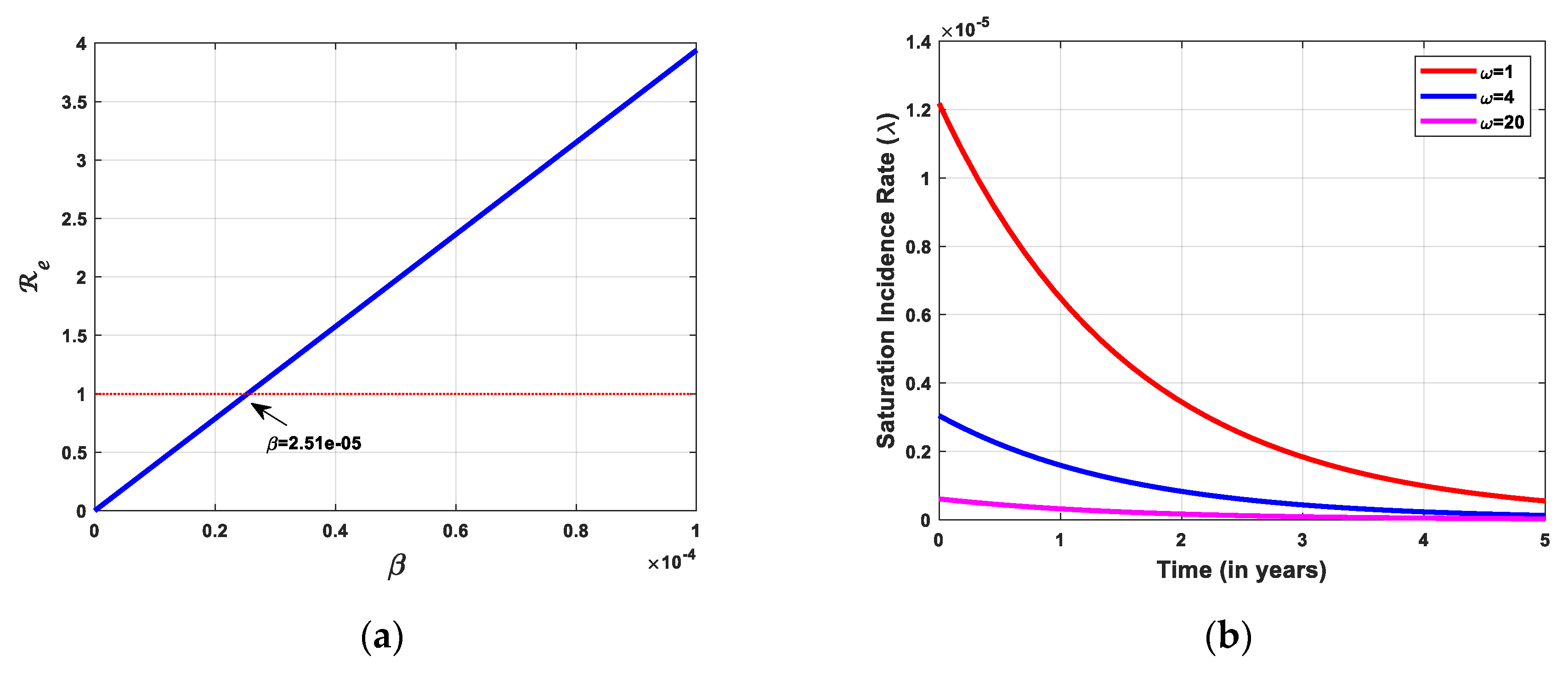
Figure 5.
Globally asymptotically stable of the DFE of model (8) in: (a) spaces; (b) spaces.
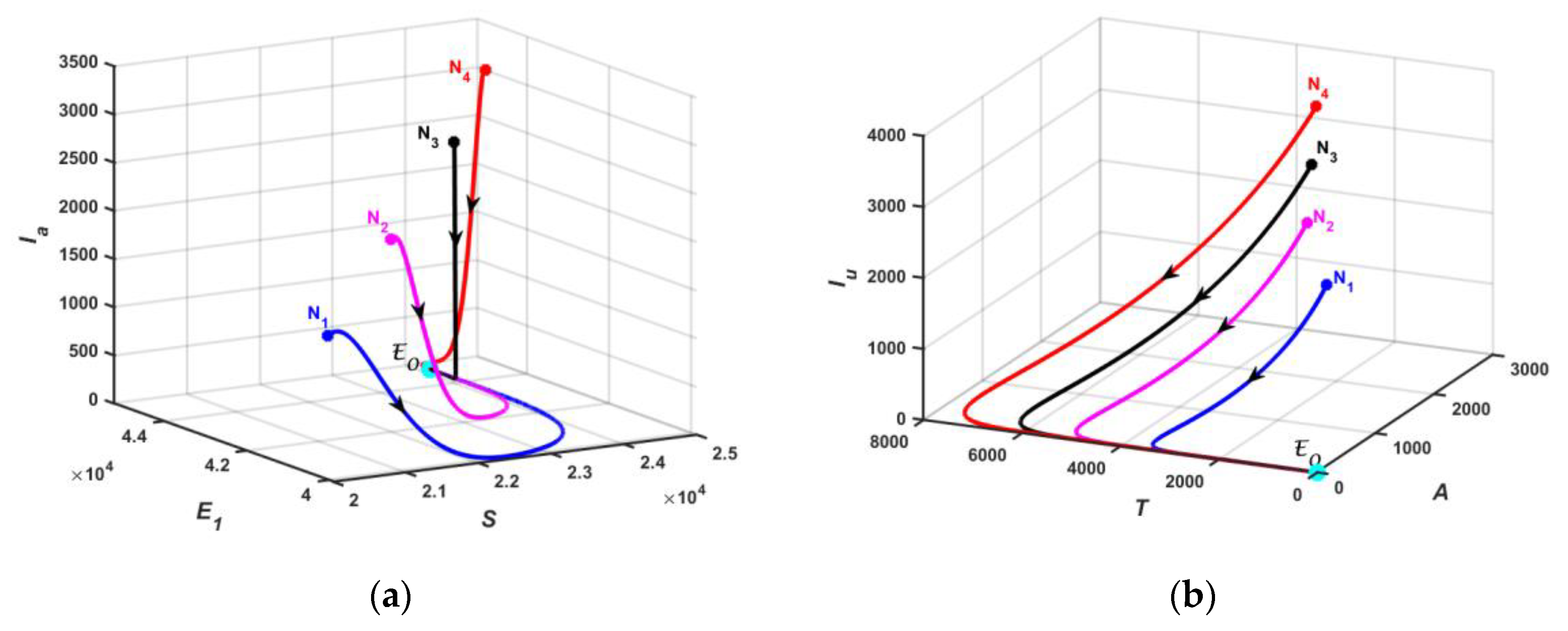
Figure 6.
Globally asymptotically stable of the EE of model (8) in: (a) spaces; (b) spaces.
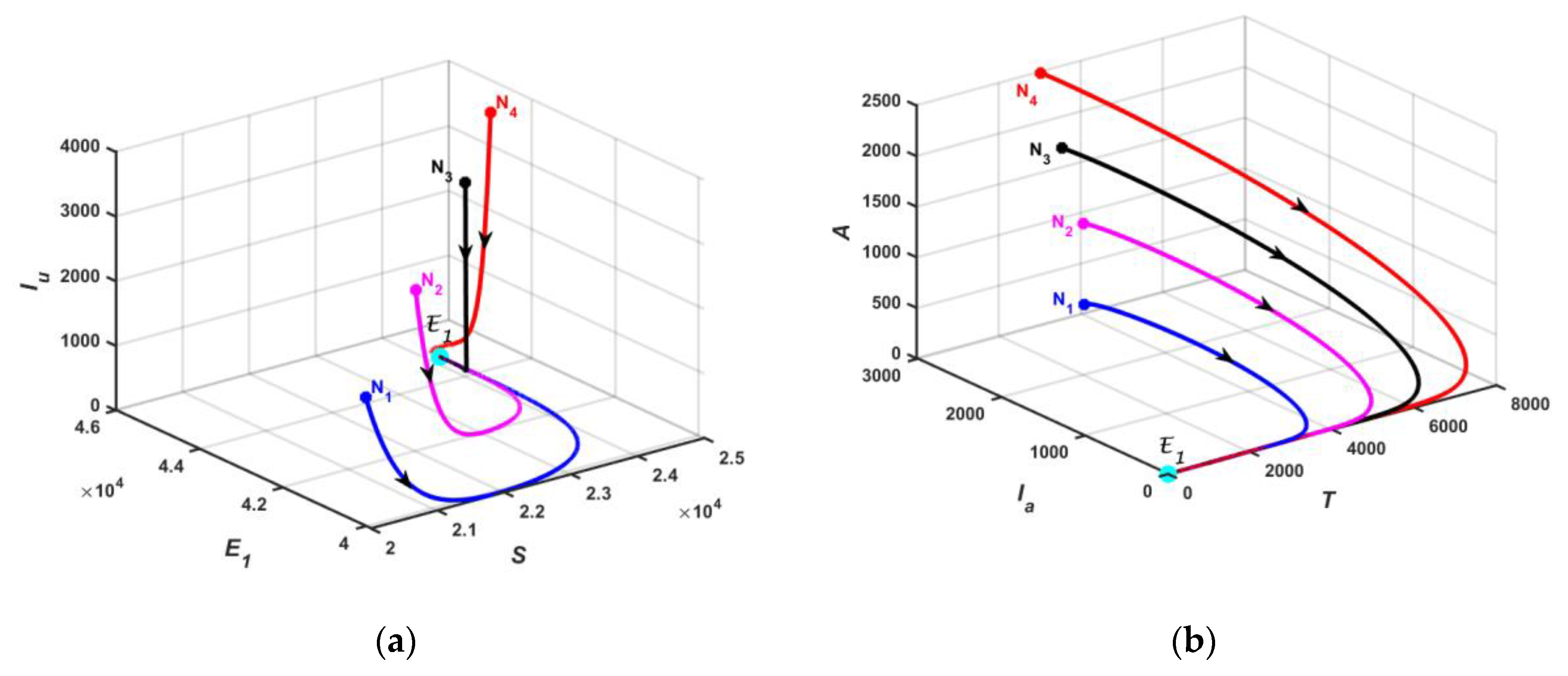
Figure 7.
Simulation of the without control and with Strategy A on: (a) the number of ; (b) the number of ; (c) the number of ; (d) control profile of and .
Figure 7.
Simulation of the without control and with Strategy A on: (a) the number of ; (b) the number of ; (c) the number of ; (d) control profile of and .
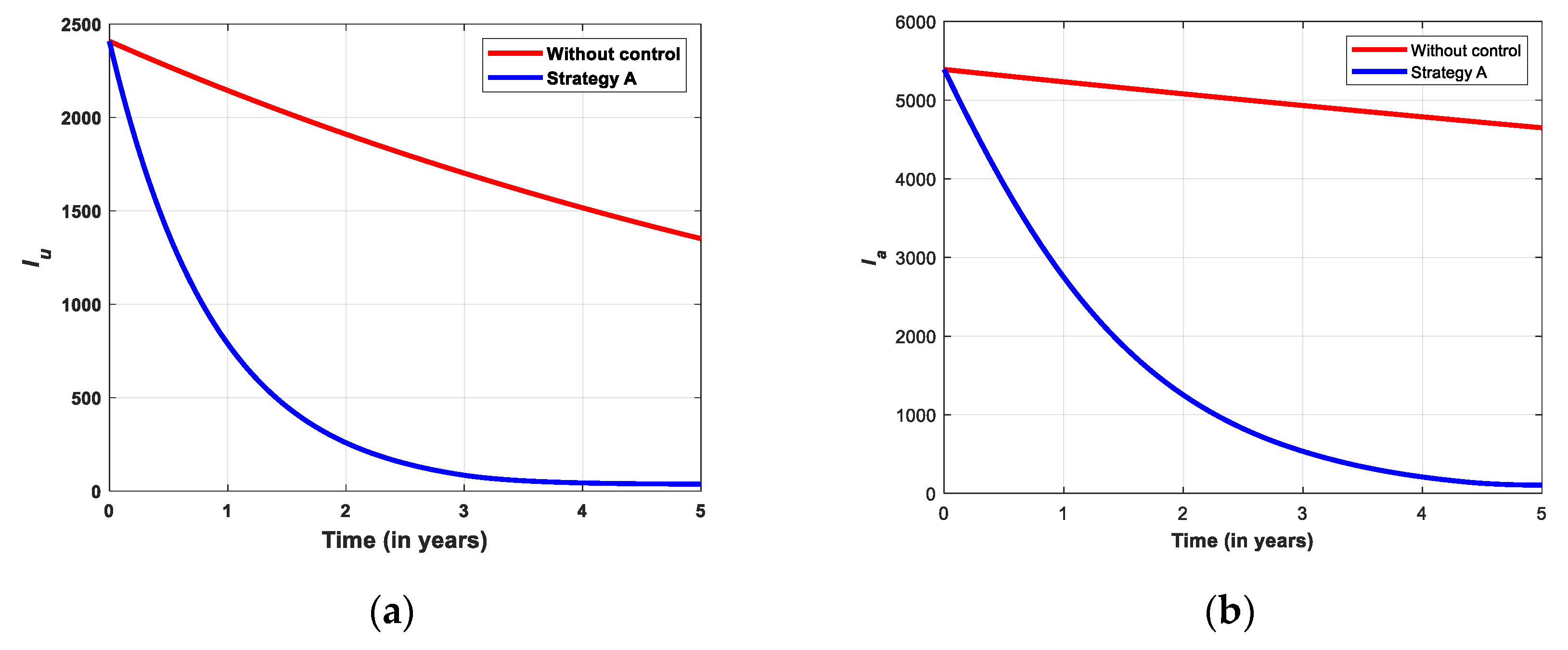
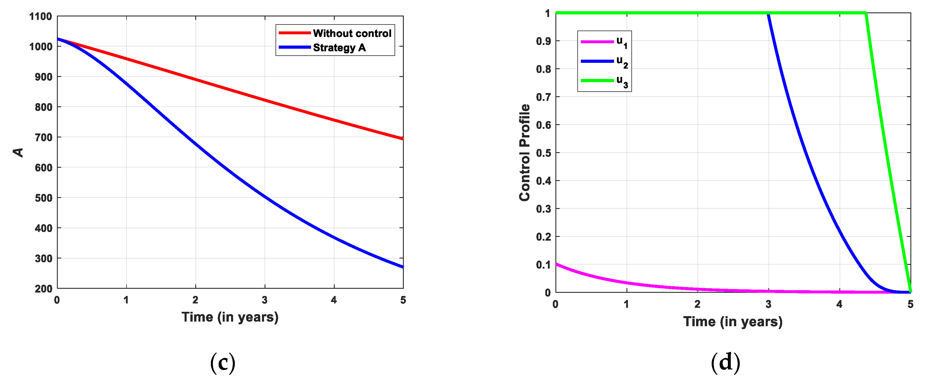
Figure 8.
Simulation of the without control and with Strategy B on: (a) the number of ; (b) the number of ; (c) the number of ; (d) control profile of and .
Figure 8.
Simulation of the without control and with Strategy B on: (a) the number of ; (b) the number of ; (c) the number of ; (d) control profile of and .
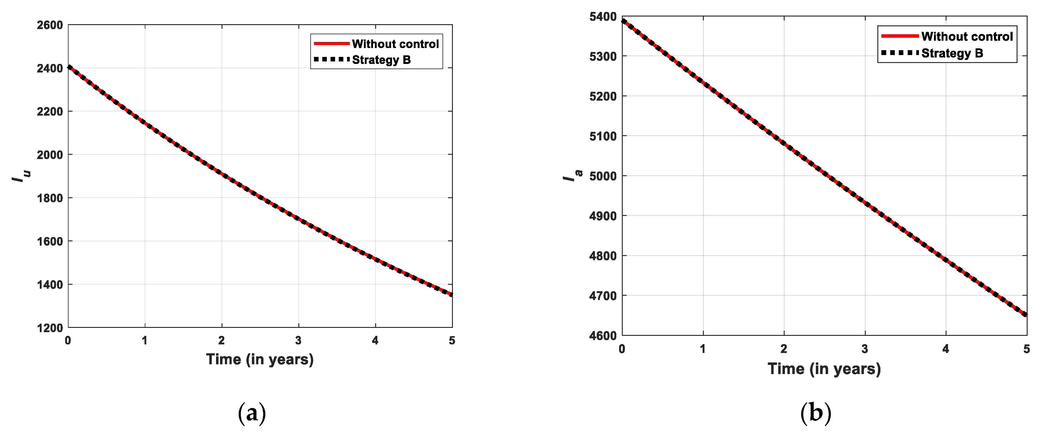
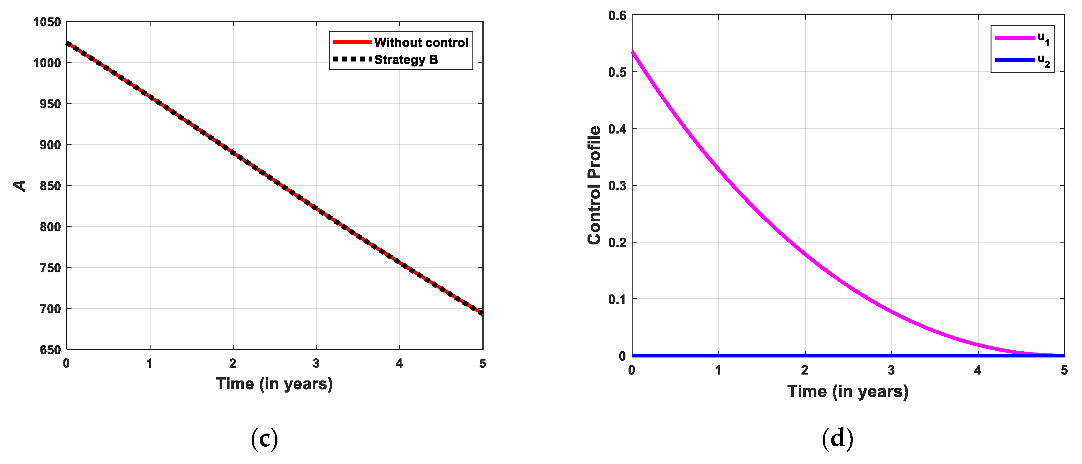
Figure 9.
Simulation of the without control and with Strategy C on: (a) the number of ; (b) the number of ; (c) the number of ; (d) control profile of and .
Figure 9.
Simulation of the without control and with Strategy C on: (a) the number of ; (b) the number of ; (c) the number of ; (d) control profile of and .
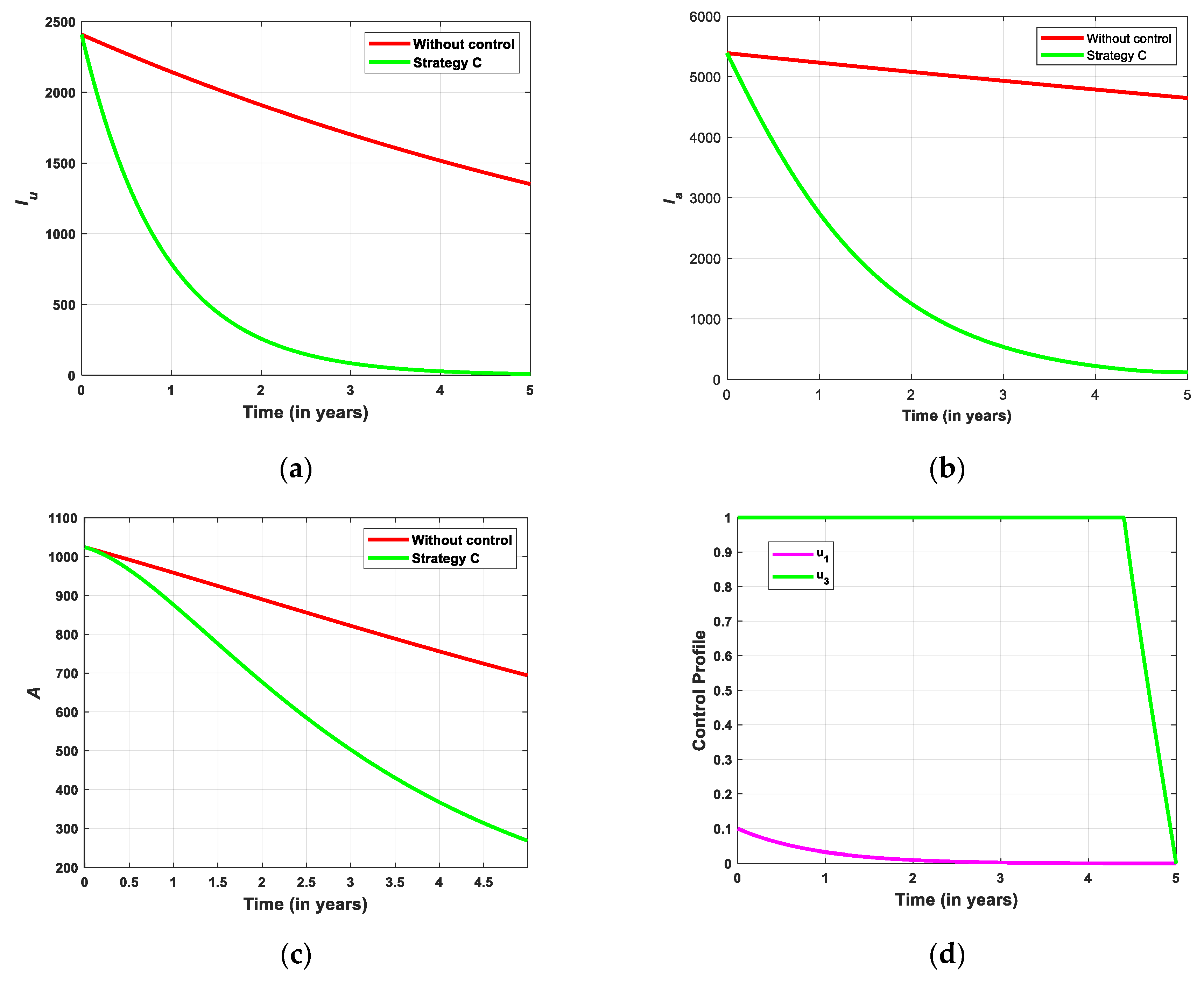
Figure 10.
Simulation of the without control and with Strategy D on: (a) the number of ; (b) the number of ; (c) the number of ; (d) control profile of and .
Figure 10.
Simulation of the without control and with Strategy D on: (a) the number of ; (b) the number of ; (c) the number of ; (d) control profile of and .
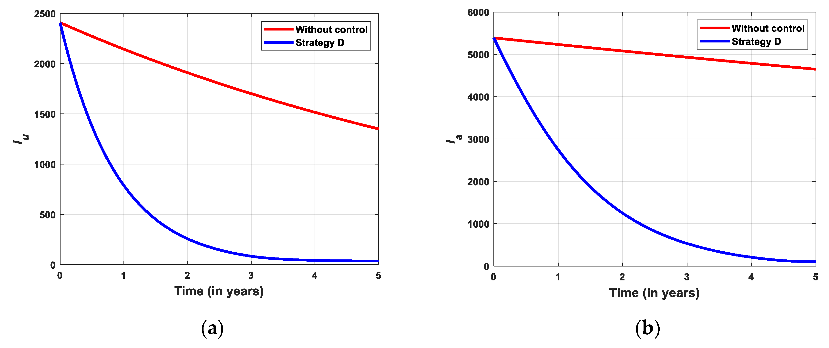
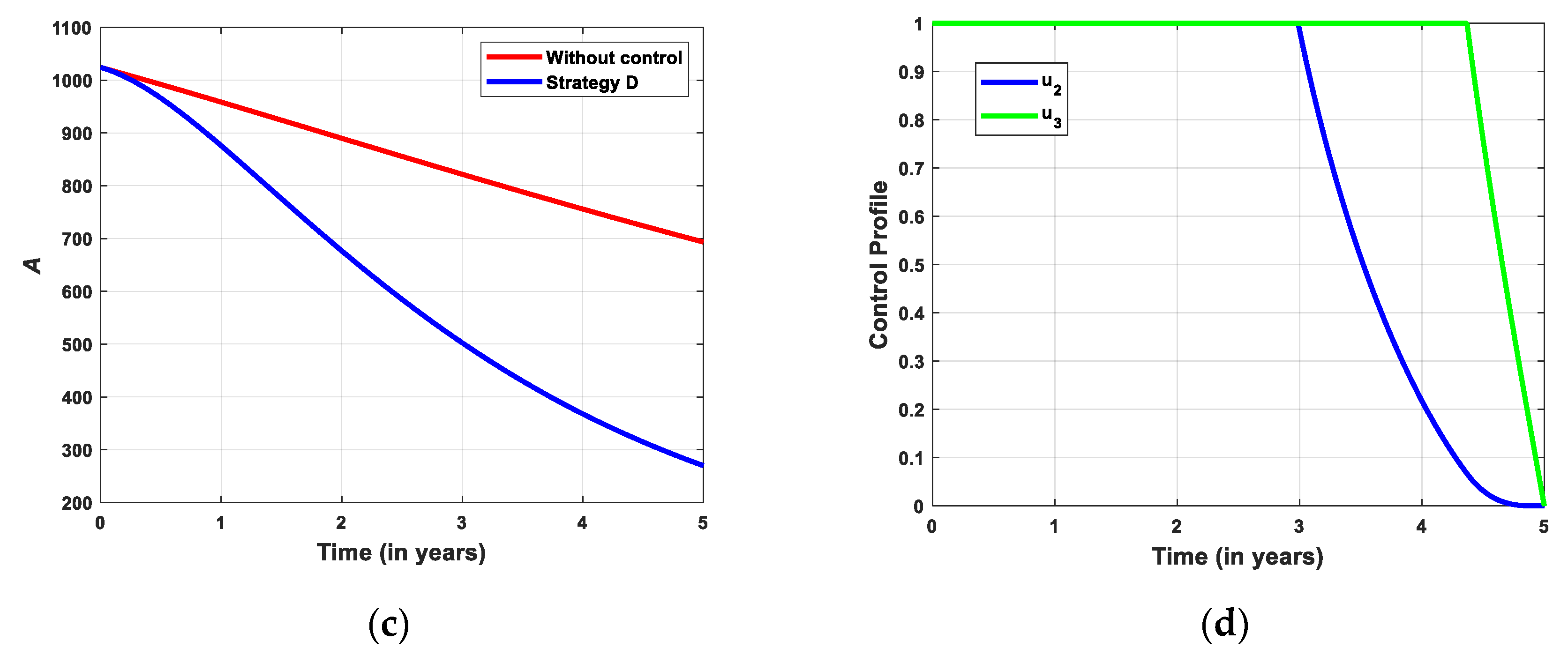

Table 1.
Description and the parameter values of the model (8).
| Parameter | Description | Value | Source |
|---|---|---|---|
| Rate of recruitment | 2000 | [6] | |
| Natural death rate | 0.0196 | [6] | |
| The rate of screening of unaware infective | 0.6 | [6] | |
| The efficiency of education campaigns in | 0.75 | Assumed | |
| The efficiency of education campaigns in | 0.6 | Assumed | |
| The rate of educating adults into E1 | 0.4 | [6] | |
| The rate of educating adults into | 0.091 | Assumed | |
| The rate of educating adults into | 0.067 | Assumed | |
| The rate of treatment of aware infectious | 0.6 | [9] | |
| Progression rate from unaware infectious to AIDS | 0.1 | [8] | |
| Progression rate from aware infectious to AIDS | 0.01 | [8] | |
| Progression rate from treated infection to AIDS | 0.001 | [8] | |
| The modification parameter relative infectivity of individuals in | 0.023 | Assumed | |
| The modification parameter relative infectivity of individuals in | 0.0016 | Assumed | |
| The rate of treatment of screened infectious | 0.33 | [6] | |
| The psychological or inhibitory effect | 4 | [10] |
Table 2.
Sensitivity indices of Re corresponding to the parameters of model (8).
| Parameter | Sensitivity Indices | Parameter | Sensitivity Indices |
|---|---|---|---|
| 1 | -0.1389 | ||
| 0.9999 | -0.0517 | ||
| -0.8083 | 0.0417 | ||
| -0.7716 | 0.0206 | ||
| -0.6925 | -0.0176 | ||
| -0.4079 | -0.0020 | ||
| -0.2605 | -0.0009 | ||
| -0.2088 |
Table 3.
Total averted infection, total cost, and ICER of Strategies B, D, A, and C.
| Strategy | TA | TC | ICER |
|---|---|---|---|
| Strategy B: | 4.7007 | 4.0169 | 0.8545 |
| Strategy D: | 25999.8318 | 526.3404 | 0.0201 |
| Strategy A: | 25999.9067 | 526.4049 | 0.8612 |
| Strategy C: | 26013.4355 | 344.4764 | -13.4475 |
Table 4.
Total averted infection, total cost, and ICER of Strategies D, A, and C.
| Strategy | TA | TC | ICER |
|---|---|---|---|
| Strategy D: | 25999.8318 | 526.3404 | 0.0202 |
| Strategy A: | 25999.9067 | 526.4049 | 0.8612 |
| Strategy C: | 26013.4355 | 344.4764 | -13.4475 |
Table 5.
Total averted infection, total cost, and ICER of Strategies D and C.
| Strategy | TA | TC | ICER |
|---|---|---|---|
| Strategy D: | 25999.8318 | 526.3404 | 0.0202 |
| Strategy C: | 26013.4355 | 344.4764 | -5.3685×10⁻⁵ |
Disclaimer/Publisher’s Note: The statements, opinions and data contained in all publications are solely those of the individual author(s) and contributor(s) and not of MDPI and/or the editor(s). MDPI and/or the editor(s) disclaim responsibility for any injury to people or property resulting from any ideas, methods, instructions or products referred to in the content. |
© 2025 by the authors. Licensee MDPI, Basel, Switzerland. This article is an open access article distributed under the terms and conditions of the Creative Commons Attribution (CC BY) license (http://creativecommons.org/licenses/by/4.0/).
Copyright: This open access article is published under a Creative Commons CC BY 4.0 license, which permit the free download, distribution, and reuse, provided that the author and preprint are cited in any reuse.


