Submitted:
02 June 2025
Posted:
03 June 2025
Read the latest preprint version here
Abstract
Residual connections are a cornerstone of modern deep neural networks, facilitating stable gradient propagation and maintaining representational expressiveness. Conventional residual formulations typically combine identity mappings and functional transformations with equal weight, without considering the input-dependent importance of each component. This uniformity restricts the model’s capability to adaptively regulate information flow. We propose a novel Contextual Modulation Training (CoMT) framework that introduces lightweight, input-dependent modulation mechanisms to dynamically modulate the functional branches of residual connections. By modulating each transformation based on the incoming data, CoMT enables fine-grained, context-aware control over information flow in the deep learning architecture. This learned modulator provides finer control than prior fixed or hand-designed scaling techniques, improving representational flexibility with a negligible cost on training scalability. CoMT is broadly applicable to architectures that employ residual connections, including ResNets and Transformers. Notably, the modulators are implemented as compact parametric functions, incurring less than 1% of the additional parameters while constantly improving the training performance. Empirical evaluations demonstrate that CoMT achieves 8%–11% perplexity reductions over baseline models across four scales of LLaMA language models, and yields substantial accuracy gains on three scales of ResNet models for image classification tasks. Along with performance improvements, we provide clear evidence that the learned modulators effectively manipulate layer-wise scaling. These findings demonstrate the effectiveness of CoMT as a general mechanism for context-sensitive residual connection modulation.
Keywords:
deep learning
; residual connection
; modulation training
; contextual scaling
1. Introduction
Deep learning has enabled advances across diverse fields, including computer vision [1,2,3], natural language processing [4,5,6,7], and scientific discovery. A key element behind its success is the ability to train increasingly deep neural networks, where depth facilitates the learning of hierarchical representations. However, increasing network dedpth often leads to optimization challenges such as vanishing gradients and degraded performance. Residual connections [1] offer an effective solution by stabilizing gradient flow, making it possible to train very deep networks. This architectural principle has since become a foundation for many modern models, from convolutional networks to Transformer-based designs.
While residual connections improve trainability, they are typically implemented in a static manner, combining identity and transformation paths equally, which does not adapt to input signals or network depth. Figure 1(a) shows the cosine similarity between input and output features for each token at each layer. The results show that: (1) the average similarity is generally around 0.2, indicating that the functional transformations produce substantially different features compared to their inputs; (2) even within the same layer, different tokens exhibit varying levels of similarity between their input and output representations. Moreover, Figure 1(b) reveals that the magnitude of transformations introduced by each layer is also highly token- and layer-dependent. These observations highlight that different inputs and different layers should have different degrees of residual modification, and therefore, an equally residual combination may not fully exploit the model’s capacity.
Recent research has emphasized the limitations of such static and identity designs. Two main branches of improvement have been explored: (1) adjusting the weighting between the residual branch and identity branch, and (2) modifying the normalization strategies applied around the residual branches. For instance, Rezero [8] introduces trainable residual scaling initialized at zero, allowing networks to start from identity mappings and gradually adapt, thus facilitating deep signal propagation without needing heavy normalization. Mix-LN [9] combines the benefits of Pre-LN and Post-LN [10], applying Post-LN to early layers to promote gradient flow and Pre-LN to later layers for stability, resulting in healthier and more effective gradient distributions across depths. LayerNorm Scaling [11] mitigates the output variance explosion problem in Pre-LN by scaling the normalization outputs according to depth, improving the contributions of deep layers during training. Dynamic Tanh (DyT) [12] offers an alternative by replacing normalization layers altogether with a learnable tanh-like activation, simplifying model design while maintaining stability.
However, most existing methods apply layer-wise normalization that is not input-aware. In contrast, the variations observed in Figure 1 indicate that a finer-grained, context-sensitive modulation could be more beneficial. This observation motivates the following question: Can residual transformations be modulated in an input-aware and depth-sensitive manner, without significantly increasing model complexity?
To address this, we propose Contextual Modulation Training (CoMT), a simple yet effective framework that introduces lightweight, input-dependent modulators into the sub-layers in residual connections. CoMT dynamically adjusts the contributions of the identity and transformation branches based on the input representations, enabling finer control over information flow throughout the network. The method requires minimal computational overhead and can be integrated into existing architectures such as ResNets and Transformers.
Empirical results across large-scale language modeling and image classification benchmarks demonstrate that CoMT consistently outperforms baseline architectures, achieving up to 5%–13.8% accuracy improvements on ResNet-50 and ResNet-152 models, and 8%–11% perplexity reductions on the LLaMA model family in comparison to the baseline models. Furthermore, analysis of the learned modulators reveals their ability to adjust layer-wise contributions in a context-sensitive manner dynamically, providing clear evidence that functional transformations in residual connections can be adaptively scaled based on the semantic characteristics of input tokens.
2. Related works
2.1. Residual connections
Training very deep neural networks is challenging due to vanishing/exploding gradients. Early solutions in recurrent models introduced gated skip connections – for example, LSTMs use a constant error carousel (an identity recurrence with weight 1) modulated by forget gates to preserve long-term gradients. Highway Networks [13] extended this concept to feed-forward networks, introducing learnable transform and carry gates, and , to blend each layer’s nonlinear transformation with its input. Residual Networks (ResNets)[1] further simplified the idea by removing explicit gating, instead directly adding a learned residual function to the input, resulting in . This reformulation enabled the successful training of convolutional networks up to 152 layers, significantly advancing the depth frontier.
One line of work has focused on making the residual connections themselves learnable or adaptive. Instead of a fixed skip connection, these methods introduce a residual weight or gate that the network can tune. The gating idea dates back to the Highway Networks’ learnable carry gates, but can be simplified. For example, Residual Gates [14] and ReZero [8] use a single scalar parameter to gate the residual branch. In ReZero, each residual block’s output is scaled by a learned coefficient , initialized to 0, before adding it back to the input:
This trivial change ensures that at initialization each layer is effectively an identity mapping ( means ), so the entire network starts as a shallow identity function. DeepNorm [15] introduced a simple change to the Post-LN Transformer: it multiplies the residual branch by a constant factor (for lower layers) when adding it to the running sum, i.e. instead of . This down-scaling strategy controls the magnitude of residual updates in early layers, preventing unstable growth of activations with depth.
2.2. Pre-LN vs. Post-LN Transformer Architectures
Batch Normalization (BN)[16] and Layer Normalization (LN)[17] are proposed to stabilize activation distributions during training. LN was soon adopted in Transformer networks [4,6,7,18], where it is applied in conjunction with residual connections to ensure stable deep training.
While the Transformer’s use of LN is essential, the placement of the LayerNorm within the residual block has profound effects on training dynamics. The original Transformer [4] is a Post-LN architecture: it applies LN after the residual addition, as described above. However, it was later shown [19] that Post-LN Transformers suffer from unstable training at large depths. Specifically, gradients at upper layers can become disproportionately large because normalization occurs after residual addition, allowing large pre-normalization activations to backpropagate unattenuated.
To address this, many modern architectures adopt a Pre-LN configuration, where LayerNorm is applied before the sub-layer transformation. In a Pre-LN Transformer, the sub-layer operates on normalized inputs, and its output is directly added to the skip connection. This strategy, used in models like GPT-2 [6] and LLaMA [7], results in more stable optimization and often eliminates the need for learning rate warm-up. However, Pre-LN comes with its own limitations. Recent studies [9,11] have pointed out a "curse of depth": deeper layers tend to contribute less to the model’s output, and can often be pruned without significant performance loss. To mitigate this, several works propose modifying Pre-LN architectures. For instance, [11] applies a depth-dependent scaling factor after Pre-LN has been suggested to dampen variance accumulation across layers. [9,20] also discuss the way to combine the Pre-LN and Post-LN by introducing the Sandwich-LN and Mix-LN.
Nevertheless, most existing normalization methods are motivated by theoretical or empirical observations and do not explicitly account for the contextual importance of residual connections on a per-input basis. As a result, these methods lack input-adaptive flexibility, limiting their ability to adjust residual pathways according to different input content dynamically.
Figure 2.
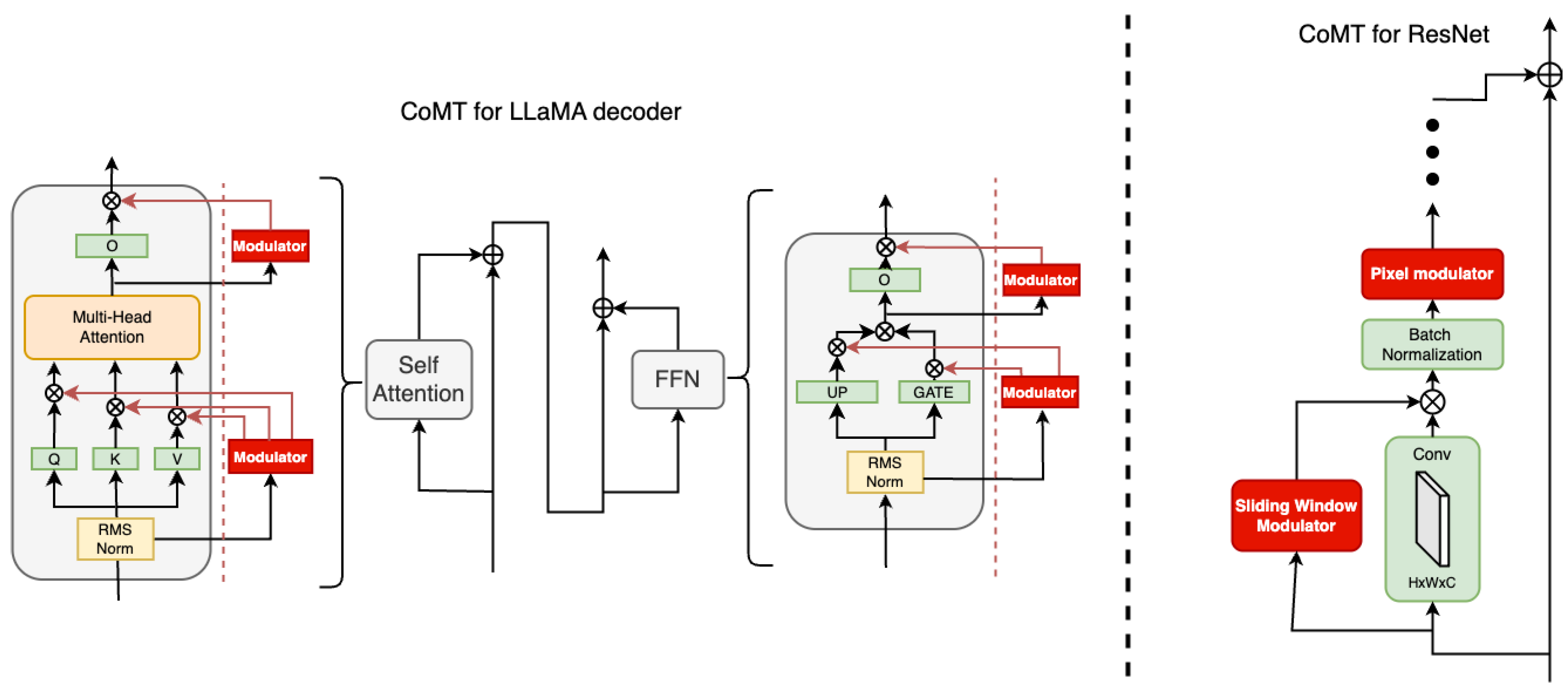
Illustration for Contextual Modulation Training (CoMT). The left panel depicts the application of CoMT to a LLaMA decoder block, which comprises a self-attention module followed by a feed-forward module. CoMT introduces modulators that dynamically scale the outputs of key linear transformations within both modules. Each linear projection is augmented with an input-aware modulator to achieve context-aware scaling. The right panel shows the application of CoMT to a ResNet convolutional block with residual connections. Two types of modulators are introduced: 1) Sliding Window Modulator: Receives the same input as the convolutional layer and outputs modulation values aligned with each sliding window, matching the spatial dimensions of the convolutional output. 2) Pixel Modulator: Replaces the traditional affine transformation in Batch Normalization with input-dependent scaling weights at the pixel level.
Figure 2.
Illustration for Contextual Modulation Training (CoMT). The left panel depicts the application of CoMT to a LLaMA decoder block, which comprises a self-attention module followed by a feed-forward module. CoMT introduces modulators that dynamically scale the outputs of key linear transformations within both modules. Each linear projection is augmented with an input-aware modulator to achieve context-aware scaling. The right panel shows the application of CoMT to a ResNet convolutional block with residual connections. Two types of modulators are introduced: 1) Sliding Window Modulator: Receives the same input as the convolutional layer and outputs modulation values aligned with each sliding window, matching the spatial dimensions of the convolutional output. 2) Pixel Modulator: Replaces the traditional affine transformation in Batch Normalization with input-dependent scaling weights at the pixel level.
3. Contextual Modulation Training
This section presents the Contextual Modulation Training (CoMT) framework, a simple yet effective mechanism for modulating functional information flow in neural networks through context-dependent scaling operations.
3.1. Preliminary: Residual Functional Composition
Modern deep architectures commonly implement residual connections by additively composing two complementary information streams: the identity data flow maintained by skip connections, and the functional transformations introduced by nonlinear modules. This standard formulation can be expressed as:
where represents parameterized transformations, such as convolutional layers, self-attention mechanisms, or feedforward networks. We refer to as the functional information flow.
Although residual connections greatly improve gradient propagation, their static composition treats all functional transformations uniformly across inputs and depths, limiting the network’s ability to adapt dynamically to varying contexts. Prior work [9,11,15] has explored heuristic scaling strategies, such as applying layer-index-dependent attenuation factors (e.g., ), but these methods lack input sensitivity and learned modulation.
To address this, CoMT introduces lightweight parametric gating mechanisms that apply dynamic, data-dependent scaling to the functional transformations:
where generates adaptive modulation coefficients, and ⊙ denotes element-wise multiplication. Unlike approaches such as LAUREL [21] that modify residual paths, CoMT preserves the original identity mappings, focusing instead on adaptively controlling the contribution of functional transformations based on input semantics.
3.2. Modulator Architecture
3.2.0.1. Contextual Adaptation
CoMT computes modulation coefficients in a token- or input-specific manner, enabling fine-grained adaptation of functional transformations across different layers and examples. Each functional sub-layer is equipped with its own lightweight modulator that dynamically adjusts its output.
3.2.0.2. MLP modulator for Transformer-based decoder.
In Transformer-based architectures, CoMT applies modulators at the level of individual linear layers rather than modulating the entire block with a single coefficient. As shown in Figure 2, for each linear projection, a small multi-layer perceptron (MLP) is used to predict a modulation weight based on the same inputs:
where and are learnable matrices, is a nonlinearity, and is the sigmoid function to constrain outputs to . Empirically, we find that setting the hidden dimension is sufficient, adding less than 0.1% to the total number of model parameters. Specifically, for the query, key, and value projections with input , the modulated computations are:
followed by attention and output projections:
For feedforward networks, modulators are similarly applied to all linear transformations:
Gradient computations for the modulated components are detailed in Appendix G.
3.3. Convolutional Modulators for ResNet Bottlenecks
For convolutional neural networks, we design two types of modulators:
Pixel-Level Modulator.
At pixel level, CoMT integrates modulation directly into batch normalization. Instead of using static affine parameters , CoMT dynamically predicts pixel-wise scaling factors based on the normalized features. The original batch normalization is:
while CoMT modifies it as:
where the first convolution projects input channels to a hidden dimension, and the second projects to a single output channel. This design enables sample-specific, pixel-wise dynamic scaling after normalization.

Table 1.
Image classification results on CIFAR-10 and CIFAR-100 using ResNet backbones. We report mean accuracy and standard error across three runs. The best results for each column are highlighted in bold. The parameter increases are also reported for each CoMT method.
Table 1.
Image classification results on CIFAR-10 and CIFAR-100 using ResNet backbones. We report mean accuracy and standard error across three runs. The best results for each column are highlighted in bold. The parameter increases are also reported for each CoMT method.
| Model | Method | CIFAR-10 | CIFAR-100 | ||
|---|---|---|---|---|---|
| Accuracy (%) ↑ | Param ↑ | Accuracy (%) ↑ | Param ↑ | ||
| ResNet-18 | Baseline | 91.12 ± 0.08 | - | 66.30 ± 0.05 | - |
| CoMT-Sliding window | 91.37 ± 0.11 | 1.43% | 66.75 ± 0.17 | 1.42% | |
| CoMT-Pixel | 91.30 ± 0.06 | 0.07% | 66.32 ± 0.09 | 0.07% | |
| ResNet-50 | Baseline | 91.10 ± 0.16 | - | 63.58 ± 0.38 | - |
| CoMT-Sliding window | 91.25 ± 0.02 | 1.89% | 64.58 ± 0.81 | 1.88% | |
| CoMT-Pixel | 91.89 ± 0.10 | 0.19% | 67.76 ± 0.01 (6.6%↑) | 0.19% | |
| ResNet-152 | Baseline | 87.93 ± 0.19 | - | 58.10 ± 0.70 | - |
| CoMT-Sliding window | 87.82 ± 0.44 | 2.19% | 59.15 ± 0.36 | 2.18% | |
| CoMT-Pixel | 90.92 ± 0.17 (4%↑) | 0.25% | 65.92 ± 0.28 (13.5%↑) | 0.25% | |
Sliding Window-Level Modulator.
At the sliding window level, CoMT modulates convolutional outputs by applying a learned scaling mask aligned with the spatial dimensions of the main convolution. The modulator structure is:
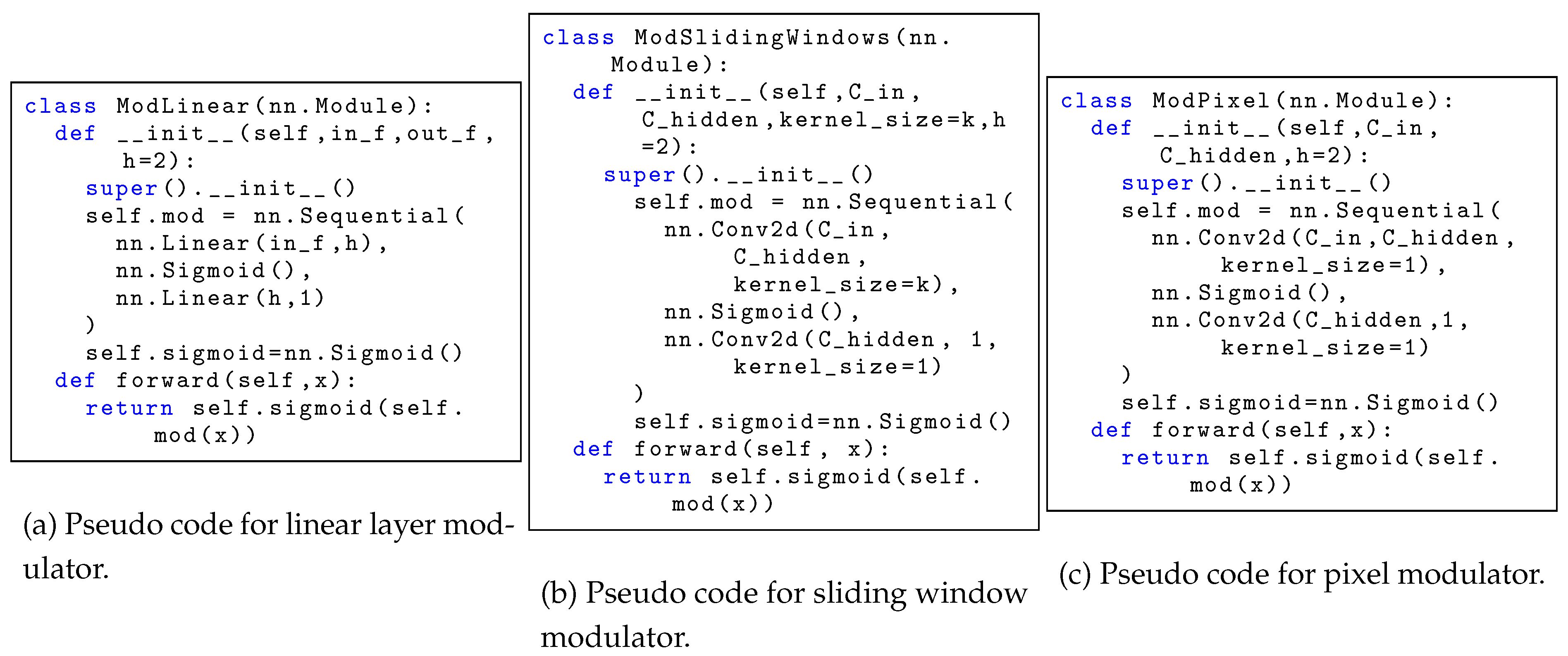
where the first convolution preserves the kernel size, stride, and padding of the modulated convolution to ensure shape alignment. This modulation allows dynamic, context-sensitive adjustment of feature transformations prior to convolution operations. Both types of convolutional modulators are illustrated in Figure 2, and the pseudo codes are shown in Figure A5.
4. Experiments
To demonstrate the effectiveness of CoMT, we evaluate it on both computer vision (CV) and natural language processing (NLP) tasks. For CV tasks, we apply CoMT to ResNet-18 [1], ResNet-50, and ResNet-152 models. For language modeling, we integrate CoMT into LLaMA [7] models ranging from 130M to 1B parameters.
4.1. CoMT for Image Classification
Experimental Setup.
We conduct experiments on CIFAR-10, CIFAR-100 [22], and ImageNet [23], using ResNet-18 [1], ResNet-50, and ResNet-152 as backbones. On CIFAR-10 and CIFAR-100, models are trained for 100 epochs with a batch size of 64, an initial learning rate of 0.01 linearly decayed to . For ImageNet, we use a one-epoch warmup, followed by cosine learning rate decay from 0.1 to , training for 90 epochs with a batch size of 512. Detailed hyperparameters are summarized in Table A6. All CIFAR experiments are repeated across three random seeds, and we report mean accuracy, standard error, and CoMT’s parameter increase ratio in Table 1.
Table 2.
Top-1 accuracy (↑) on ImageNet with ResNet backbones.
| Model | ResNet-18 | ResNet-50 | ResNet-152 |
|---|---|---|---|
| Baseline | 67.71 | 72.33 | 73.10 |
| CoMT-Sliding window | 68.17 | 72.83 | 73.65 |
| CoMT-Pixel | 68.02 | 72.97 | 74.01 |
Main Results.
Table 1 summarizes the image classification results except for ResNet-152 on CIFAR10. Both pixel-level and sliding-window CoMT variants consistently improve performance across models and datasets. Notably, on deeper architectures like ResNet-50 and ResNet-152, pixel-level CoMT yields stronger gains with negligible parameter increase (around 0.2%).
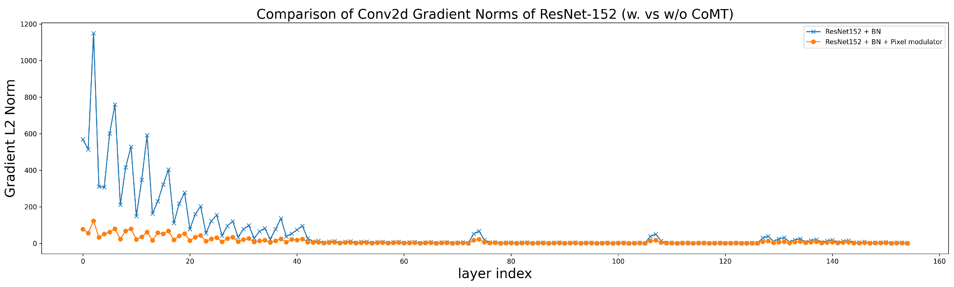
Additionally, even with residual connections and batch normalization, deeper models such as ResNet-50 and ResNet-152 underperform ResNet-18 on CIFAR10 and CIFAR100, indicating that merely increasing depth without adaptive scaling can reduce learning efficiency. Integrating CoMT significantly narrows this gap: pixel-level CoMT improves ResNet-152 on CIFAR-100 by 13.5% over the baseline. Gradient flow analysis in Figure 3 shows that CoMT stabilizes early gradients across depth, facilitating smoother optimization in deep residual networks.
We further conduct a sensitivity analysis on the hidden size of the convolutional modulators, summarized in Table A7. For sliding-window modulators, the hidden size is adaptively determined based on the input channel dimensions, while for pixel-level modulators, a fixed hidden size is employed. The results indicate that increasing the hidden size yields only marginal improvements; the primary performance gains stem from the introduction of contextual modulation itself rather than the specific choice of hidden dimension.
Finally, Table 2 reports the ImageNet results. CoMT consistently achieves performance improvements over the baseline models with minimal additional parameter cost, further validating its effectiveness across large-scale datasets.
4.2. CoMT for Language Modeling
Experimental Setup.
We evaluate CoMT on natural language processing tasks via language modeling on the LLaMA model family ranging from 130M to 1B parameters on the C4 dataset [24], using the experimental scripts and settings provided by [11]. We employ the Adam optimizer [25], with a learning rate of for models up to 350M parameters and for the 1B parameter model. CoMT introduces a single additional hyperparameter—the hidden dimension of the modulator. Throughout experiments shown in Table 3, we set the hidden dimension to 2. We also conduct a sensitivity analysis on the hidden dimension, as shown in Table 5, observing that while increasing the hidden size yields marginal improvements, the primary performance gains of CoMT stem from the introduction of contextual modulation rather than from larger hidden dimensions.
Main Results for Language Modeling.
Table 3 compares perplexities achieved by various normalization strategies on LLaMA models of different scales. Across all settings, our proposed CoMT consistently outperforms prior approaches, achieving the lowest perplexity on every model size.
Table 3.
Perplexity (↓) comparison of various layer normalization methods across various LLaMA sizes. The original LLaMA model is the Pre-LN, which we term the baseline method. The best results for each column are highlighted in bold.
Table 3.
Perplexity (↓) comparison of various layer normalization methods across various LLaMA sizes. The original LLaMA model is the Pre-LN, which we term the baseline method. The best results for each column are highlighted in bold.
| LLaMA-130M | LLaMA-250M | LLaMA-350M | LLaMA-1B | |
| Training Tokens | 2.2B | 3.9B | 6.0B | 8.9B |
| Post-LN | 26.95 | 1409.79 | 1368.33 | 1390.75 |
| DeepNorm | 27.17 | 22.77 | 1362.59 | 1409.08 |
| Post-LN + CoMT | 26.69 | 21.45 | 19.11 | 17.68 |
| Mix-LN | 26.07 | 21.39 | 1363.21 | 1414.78 |
| Pre-LN (baseline) | 26.73 | 21.92 | 19.58 | 17.02 |
| Pre-LN + LayerNorm Scaling | 25.76 | 20.35 | 18.20 | 15.71 |
| Pre-LN + CoMT | 23.77 (11.07%↓) | 19.74 (9.95%↓) | 17.98 (8.17%↓) | 15.08 (11.40%↓) |
Moreover, we implement CoMT on both Pre-LN and Post-LN scenarios. Notably, traditional Post-LN exhibits severe degradation as model size increases, reflecting known instability issues in deep transformers when normalization is applied post-residual addition [11,15]. DeepNorm, which also gives learnable scaling weights to the sublayers of the residual parts, also crushed down on larger-scale models like LLaMA-350M and LLaMA-1b. The reason could be that although it gives a careful initialization, it remains input-agnostic and static, limiting its capacity for adaptive feature modulation.
In contrast, CoMT directly addresses these limitations by introducing fine-grained, token-specific modulation of functional residual pathways, enabling dynamic adaptation to input semantics without disrupting identity-preserving residual flows. By learning contextual scaling gates jointly with network parameters, CoMT allows the model to amplify or suppress feature transformations based on the content of each input, resulting in more effective gradient flow and better feature utilization throughout depth. Therefore, even incorporating the Post-LN, CoMT is still able to stabilize the training even when the layers go deep. Empirically, compared to the original model with Post-LN and Pre-LN, CoMT achieves substantial perplexity reductions. In addition, CoMT outperforms the strongest previous baseline at all scales.
Table 4.
Ablation study on modulators on different functional modules for CoMT.
| Modules | LLaMA60M | LLaMA130M |
|---|---|---|
| Baseline | 33.28 | 26.07 |
| self-attention | 34.86 | 25.21 |
| mlp | 33.35 | 24.40 |
| only_last | 32.96 | 24.47 |
| only_first | 32.71 | 24.10 |
| only_qk | 33.67 | 24.74 |
| all | 32.69 | 23.77 |
Table 5.
Ablation study on modulator hidden dimension for CoMT.
| Hidden Size | LLaMA60M | LLaMA130M |
|---|---|---|
| Baseline | 33.28 | 26.07 |
| 2 | 32.69 | 23.83 |
| 4 | 32.58 | 23.76 |
| 8 | 32.21 | 23.72 |
| 16 | 32.56 | 23.82 |
| 32 | 32.36 | 23.59 |
Contribution of Functional Components.
To investigate the contribution of different components to functional flow, we selectively apply CoMT modulators to individual modules within each decoder. Table 4 summarizes the ablation results on LLaMA-60M and LLaMA-130M models. As shown in Table 4, applying modulators to all components (“all”) consistently yields the best perplexity on both LLaMA-60M and LLaMA-130M, indicating that full-path modulation provides the most comprehensive control over residual transformation dynamics.
Interestingly, selectively modulating only the query and key projections (“only_qk”) or applying modulation solely to the self-attention block (“self-attention”) yields inconsistent results across model scales and, in the case of LLaMA-60M, even underperforms the baseline. This suggests that partial modulation within isolated components may disrupt the balance of residual information flow. In contrast, modulating only the output layers (“only_last,” including o_proj and down_proj) or only the input layers (“only_first,” including q_proj, k_proj, v_proj, up_proj, and gate_proj) leads to moderate improvements, demonstrating that both early and late transformations contribute to effective modulation. Nevertheless, the best performance is consistently achieved when modulators are applied to all layers within each block. These findings emphasize that CoMT’s strength lies in its comprehensive, token-aware modulation across the full residual transformation path, encompassing both the attention and feedforward modules.
Effect of Modulator Hidden Size.
We further analyze the impact of the hidden dimension of the MLP modulator. Table 5 presents the results for various hidden sizes. Even with a minimal hidden dimension of 2, CoMT already delivers substantial improvements over the baseline. Increasing the hidden size from 2 to 32 provides marginal but consistent gains, suggesting that very lightweight modulators are sufficient to capture essential input-dependent scaling behavior. This efficiency validates the design goal of CoMT: achieving fine-grained functional modulation with minimal additional parameter overhead.
5. Contextual Modulator Values Analysis
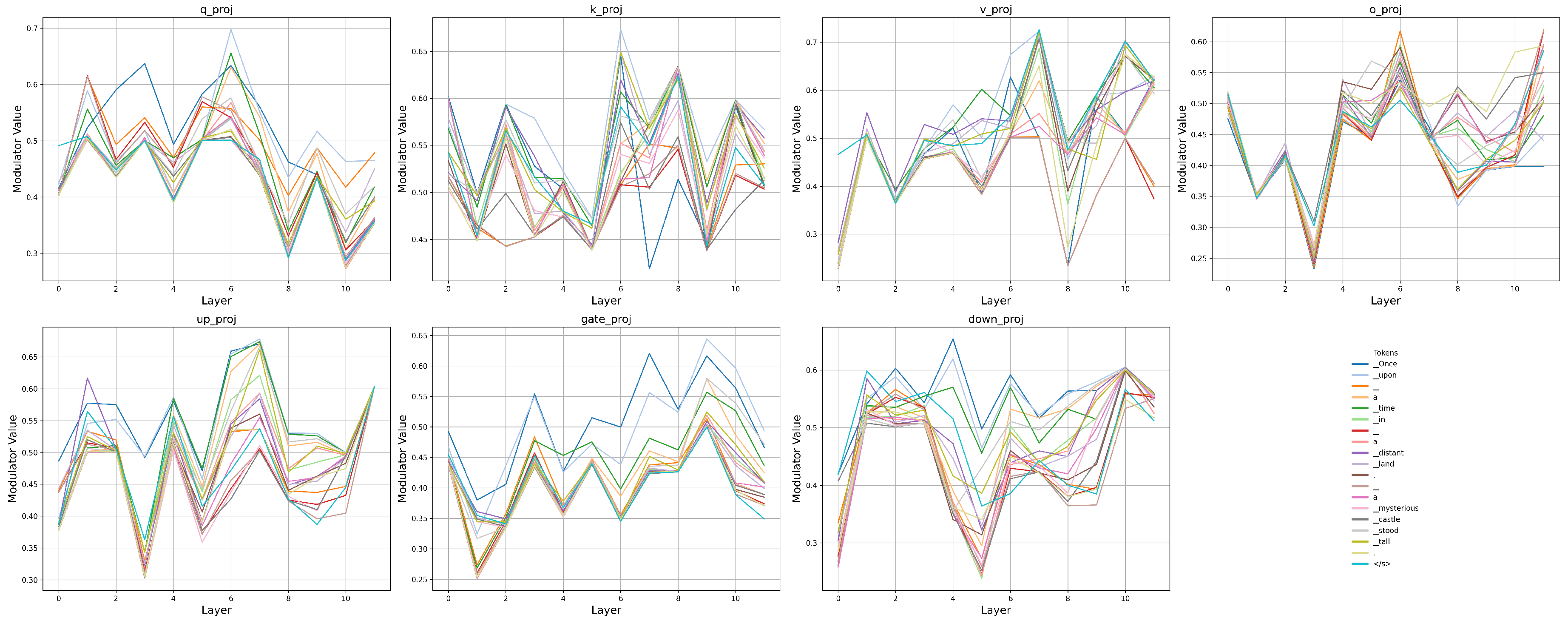
The results shown in Section 4 highlight that, beyond static architectural scaling such as fixed layer normalization strategies, context/input-sensitive modulation offers a powerful new direction for improving optimization and expressivity in deep language or vision models. CoMT is learning modulation weights for each input per sub-layer in the functional residual connections. Therefore, the key point is whether they are really able to capture the contextual information. Figure 4 illustrates the modulator values across all layers and major modules (q_proj, k_proj, v_proj, o_proj, up_proj, gate_proj, down_proj) of the LLaMA-130M model that was pretrained with CoMT for a given sequence of input tokens.
Layer-wise modulation.
Across all subplots, modulator values vary systematically with depth, demonstrating that the scaling factors are not static but adapt dynamically as a function of layer index. For instance, the modulator values exhibit sharp transitions around layers 3 and 8, which are consistently seen across different modules and tokens. This behavior suggests that the modulators successfully capture diverse hierarchical representations along the network depth, enabling fine-grained control over layer-wise computation.
Module-wise modulation.
Comparing across modules, we see that different modules exhibit distinct modulation patterns even for the same token input. For example, while q_proj and k_proj display relatively moderate variance across layers, v_proj and up_proj present higher peaks at deeper layers, reflecting differentiated functional importance and sensitivity among modules. This module-specific adaptivity highlights that the learned modulators are sensitive not only to position in the network but also to the semantic role of each component.
Token-wise modulation.
Even within a fixed module and layer, different input tokens induce distinct modulator values. For instance, tokens like _Once and _castle tend to generate higher modulation weights in early and middle layers, whereas punctuation tokens such as . and </s> maintain relatively lower and flatter modulations. This indicates that the modulators are able to adapt to the content and context of individual tokens, dynamically adjusting computation pathways based on semantic and syntactic cues.
Figure 4.
Token-wise modulator values across layers and modules in a LLaMA-130M model trained with CoMT. Each subplot corresponds to a specific linear projection of the decoder layer. The plotted curves represent different tokens from the input sequence.
Figure 4.
Token-wise modulator values across layers and modules in a LLaMA-130M model trained with CoMT. Each subplot corresponds to a specific linear projection of the decoder layer. The plotted curves represent different tokens from the input sequence.
6. Conclusion
This work introduces Contextual Modulation Training (CoMT), a general framework for improving the adaptability of residual connections through lightweight, input-dependent layer-wise modulation training mechanisms. By modulating each functional transformation according to its contextual input, CoMT enables fine-grained, context-aware layer-wise scaling control in the deep learning architecture with the residual connections.
We validate CoMT across both vision and language domains, demonstrating consistent improvements in performance over baseline models on CIFAR-10, CIFAR-100, ImageNet, and LLaMA language models. Analysis of the learned modulators reveals that CoMT achieves fine-grained, context-sensitive scaling at the level of layers, modules, and tokens, supporting more efficient and expressive feature transformations across depth.
Importantly, CoMT achieves these benefits with minimal computational overhead, making it practical for large-scale training. These findings suggest that context-aware residual modulation is a promising direction for advancing the optimization and representational power of deep learning architectures.
Future work includes extending CoMT to larger-scale pretraining regimes, exploring different architectures beyond ResNets and Transformers, and investigating theoretical foundations for optimal modulator design.
Acknowledge
This work was supported by the Zhou Yahui Chair Professorship award of Tsinghua University (to CVC), the National High-Level Talent Program of the Ministry of Science and Technology of China (grant number 20241710001, to CVC). This work was also supported by the Ant group.
Appendix G Gradient computation of each part in LLaMA
The modulation gates influence parameter updates through element-wise scaling of gradient components. For attention projection matrices:
Table A6.
Hyperparameters of ResNet-18, ResNet-50, and ResNet-152 on Image Classification Tasks.
| Hyper-parameter | CIFAR10 & CIFAR100 | ImageNet |
| Batch Size | 64 | 512 |
| Training Epochs | 100 | 90 |
| LR Decay Method | Linear | Cosine |
| Start Learning Rate | 0.01 | 0.1 |
| End Learning Rate | 0.0001 | 0.001 |
| Momentum | 0.9 | 0.9 |
| Weight decay | 0 | 0 |
For feed-forward layers, the gradients of each weight matrix are computed by:
Figure A5.
Three variations of modulators of CoMT.
Appendix H Broader Impact
In this work, we introduce a novel methodology for modulating the scaling of the functional transformations to be merged into the skip connections of inputs. The goal of this article is to enhance the performance of AI model training. However, the widespread availability of advanced artificial neural networks, particularly large language models (LLMs), also presents risks of misuse. It is essential to carefully consider and manage these factors to maximize benefits and minimize risks.
Table A7.
Image classification results on CIFAR-10 and CIFAR-100 using ResNet backbones. We report mean accuracy and standard error across three runs. The best results for each column are highlighted in bold.
Table A7.
Image classification results on CIFAR-10 and CIFAR-100 using ResNet backbones. We report mean accuracy and standard error across three runs. The best results for each column are highlighted in bold.
| Model | CIFAR-10 | CIFAR-100 | ||
|---|---|---|---|---|
| Accuracy (↑) | Param ↑ | Accuracy (↑) | Param ↑ | |
| ResNet-18 | ||||
| Baseline | 91.12 ± 0.08 | - | 66.30 ± 0.05 | - |
| CoMT-Sliding window (1/16) | 91.37 ± 0.06 | 5.72% | 66.78 ± 0.27 | 5.69% |
| CoMT-Sliding window (1/32) | 91.44 ± 0.18 (0.35%↑) | 2.86% | 66.90 ± 0.21 (0.9%↑) | 2.84% |
| CoMT-Sliding window (1/64) | 91.37 ± 0.11 | 1.43% | 66.75 ± 0.17 | 1.42% |
| CoMT-Pixel (2) | 91.30 ± 0.06 | 0.07% | 66.32 ± 0.09 | 0.07% |
| CoMT-Pixel (4) | 90.98 ± 0.08 | 0.14% | 66.14 ± 0.09 | 0.14% |
| CoMT-Pixel (8) | 91.20 ± 0.11 | 0.28% | 66.44 ± 0.06 | 0.27% |
| ResNet-50 | ||||
| Baseline | 91.10 ± 0.16 | - | 63.58 ± 0.38 | - |
| CoMT-Sliding window (1/16) | 90.54 ± 0.08 | 7.58% | 63.98 ± 0.14 | 7.52% |
| CoMT-Sliding window (1/32) | 90.77 ± 0.11 | 3.79% | 63.77 ± 0.32 | 3.76% |
| CoMT-Sliding window (1/64) | 91.25 ± 0.02 | 1.89% | 64.58 ± 0.81 | 1.88% |
| CoMT-Pixel (2) | 91.89 ± 0.10 | 0.19% | 67.76 ± 0.01 (6.6%↑) | 0.19% |
| CoMT-Pixel (4) | 92.00 ± 0.07 (1%↑) | 0.39% | 67.61 ± 0.15 | 0.38% |
| CoMT-Pixel (8) | 91.84 ± 0.05 | 0.77% | 67.17 ± 0.08 | 0.77% |
| ResNet-152 | ||||
| Baseline | 87.93 ± 0.19 | - | 58.10 ± 0.70 | - |
| CoMT-Sliding window (1/16) | 87.45 ± 0.21 | 8.75% | 58.48 ± 0.79 | 8.72% |
| CoMT-Sliding window (1/32) | 88.12 ± 0.56 | 4.37% | 59.25 ± 0.92 | 4.36% |
| CoMT-Sliding window (1/64) | 87.82 ± 0.44 | 2.19% | 59.15 ± 0.36 | 2.18% |
| CoMT-Pixel (2) | 90.92 ± 0.17 | 0.25% | 65.92 ± 0.28 | 0.25% |
| CoMT-Pixel (4) | 91.23 ± 0.10 (3.8%↑) | 0.49% | 66.14 ± 0.20 (13.8%↑) | 0.49% |
| CoMT-Pixel (8) | 90.43 ± 0.07 | 1.04% | 65.89 ± 0.18 | 0.99% |
Appendix I Experiments compute resources
All experiments were conducted on NVIDIA A100 80GB GPUs. The three ResNet models on CIFAR10 and CIFAR100 were trained using a single GPU, while the training on ImageNet and the large language model results were trained using eight GPUs in parallel.
References
- He, K.; Zhang, X.; Ren, S.; Sun, J. Deep residual learning for image recognition. In Proceedings of the Proceedings of the IEEE conference on computer vision and pattern recognition, 2016, pp. 770–778.
- Tan, M.; Le, Q. Efficientnet: Rethinking model scaling for convolutional neural networks. In Proceedings of the International conference on machine learning. PMLR, 2019, pp. 6105–6114.
- Liu, Z.; Lin, Y.; Cao, Y.; Hu, H.; Wei, Y.; Zhang, Z.; Lin, S.; Guo, B. Swin transformer: Hierarchical vision transformer using shifted windows. In Proceedings of the Proceedings of the IEEE/CVF international conference on computer vision, 2021, pp. 10012–10022.
- Vaswani, A.; Shazeer, N.; Parmar, N.; Uszkoreit, J.; Jones, L.; Gomez, A.N.; Kaiser, Ł.; Polosukhin, I. Attention is all you need. Advances in neural information processing systems 2017, 30.
- Devlin, J.; Chang, M.W.; Lee, K.; Toutanova, K. BERT: Pre-training of Deep Bidirectional Transformers for Language Understanding, 2019, [arXiv:cs.CL/1810.04805].
- Radford, A.; Narasimhan, K.; Salimans, T.; Sutskever, I. Improving Language Understanding by Generative Pre-Training. https://cdn.openai.com/research-covers/language-unsupervised/language_understanding_paper.pdf, 2018.
- Touvron, H.; Lavril, T.; Izacard, G.; Martinet, X.; Lachaux, M.A.; Lacroix, T.; Rozière, B.; Goyal, N.; Hambro, E.; Azhar, F.; et al. Llama: Open and efficient foundation language models. arXiv preprint arXiv:2302.13971 2023.
- Bachlechner, T.; Majumder, B.P.; Mao, H.; Cottrell, G.; McAuley, J. Rezero is all you need: Fast convergence at large depth. In Proceedings of the Uncertainty in Artificial Intelligence. PMLR, 2021, pp. 1352–1361.
- Li, P.; Yin, L.; Liu, S. Mix-ln: Unleashing the power of deeper layers by combining pre-ln and post-ln. arXiv preprint arXiv:2412.13795 2024.
- Nguyen, T.Q.; Salazar, J. Transformers without tears: Improving the normalization of self-attention. arXiv preprint arXiv:1910.05895 2019.
- Sun, W.; Song, X.; Li, P.; Yin, L.; Zheng, Y.; Liu, S. The Curse of Depth in Large Language Models. arXiv preprint arXiv:2502.05795 2025.
- Zhu, J.; Chen, X.; He, K.; LeCun, Y.; Liu, Z. Transformers without normalization. arXiv preprint arXiv:2503.10622 2025.
- Srivastava, R.K.; Greff, K.; Schmidhuber, J. Highway Networks, 2015, [arXiv:cs.LG/1505.00387].
- Savarese, P.; Figueiredo, D. Residual gates: A simple mechanism for improved network optimization. In Proceedings of the Proc. Int. Conf. Learn. Representations, 2017.
- Wang, H.; Ma, S.; Dong, L.; Huang, S.; Zhang, D.; Wei, F. Deepnet: Scaling transformers to 1,000 layers. IEEE Transactions on Pattern Analysis and Machine Intelligence 2024.
- Ioffe, S.; Szegedy, C. Batch normalization: Accelerating deep network training by reducing internal covariate shift. In Proceedings of the International conference on machine learning. pmlr, 2015, pp. 448–456.
- Ba, J.L.; Kiros, J.R.; Hinton, G.E. Layer normalization. arXiv preprint arXiv:1607.06450 2016.
- DeepSeek-AI. DeepSeek-R1: Incentivizing Reasoning Capability in LLMs via Reinforcement Learning, 2025, [arXiv:cs.CL/2501.12948].
- Xiong, R.; Yang, Y.; He, D.; Zheng, K.; Zheng, S.; Xing, C.; Zhang, H.; Lan, Y.; Wang, L.; Liu, T.Y. On Layer Normalization in the Transformer Architecture, 2020, [arXiv:cs.LG/2002.04745].
- Ding, M.; Yang, Z.; Hong, W.; Zheng, W.; Zhou, C.; Yin, D.; Lin, J.; Zou, X.; Shao, Z.; Yang, H.; et al. CogView: Mastering Text-to-Image Generation via Transformers, 2021, [arXiv:cs.CV/2105.13290].
- Menghani, G.; Kumar, R.; Kumar, S. LAUREL: Learned Augmented Residual Layer. arXiv preprint arXiv:2411.07501 2024.
- Krizhevsky, A. Learning Multiple Layers of Features from Tiny Images 2009. pp. 32–33.
- Russakovsky, O.; Deng, J.; Su, H.; Krause, J.; Satheesh, S.; Ma, S.; Huang, Z.; Karpathy, A.; Khosla, A.; Bernstein, M.; et al. ImageNet Large Scale Visual Recognition Challenge. International Journal of Computer Vision (IJCV) 2015, 115, 211–252. [CrossRef]
- Raffel, C.; Shazeer, N.; Roberts, A.; Lee, K.; Narang, S.; Matena, M.; Zhou, Y.; Li, W.; Liu, P.J. Exploring the Limits of Transfer Learning with a Unified Text-to-Text Transformer. Journal of Machine Learning Research 2020, 21, 1–67.
- Kingma, D.P.; Ba, J. Adam: A Method for Stochastic Optimization, 2017, [arXiv:cs.LG/1412.6980].
Figure 1.
Angular distance and L2 norm ratio across decoder layers for an example sentence in a pretrained LLaMA2-7B model. (a) Cosine similarity between input and output representations at each decoder layer, per token. (b) L2 norm ratio (output divided by input norm) across layers. The tokenized input sequence is shown for reference.
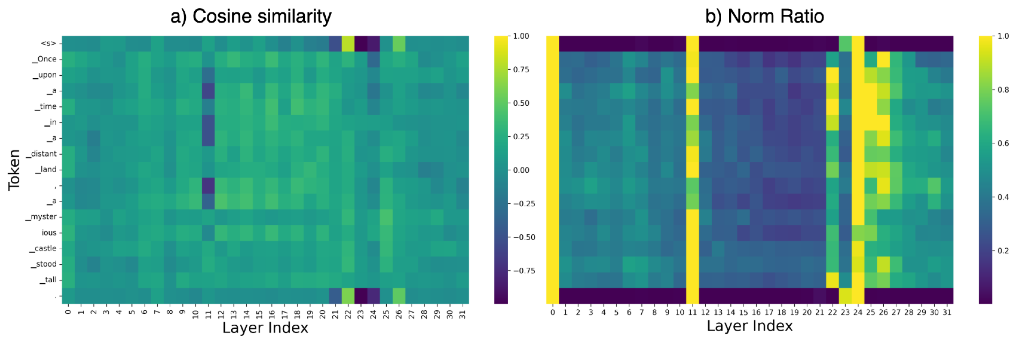
Figure 3.
Gradient stability analysis of ResNet-152. We compare the L2 norm of Conv2d gradients across layers for the standard model with BatchNorm (blue) and the model augmented with our pixel-level CoMT modulator (orange). CoMT effectively suppresses the large gradient spikes observed in early layers, indicating improved gradient flow and training stability, especially during the initial training phase.
Disclaimer/Publisher’s Note: The statements, opinions and data contained in all publications are solely those of the individual author(s) and contributor(s) and not of MDPI and/or the editor(s). MDPI and/or the editor(s) disclaim responsibility for any injury to people or property resulting from any ideas, methods, instructions or products referred to in the content. |
© 2025 by the authors. Licensee MDPI, Basel, Switzerland. This article is an open access article distributed under the terms and conditions of the Creative Commons Attribution (CC BY) license (http://creativecommons.org/licenses/by/4.0/).
Copyright: This open access article is published under a Creative Commons CC BY 4.0 license, which permit the free download, distribution, and reuse, provided that the author and preprint are cited in any reuse.


